Delay-Adaptive Federated Filtering with Online Model Calibration for Deep-Space Multi-Spacecraft Orbit Determination

1. Introduction

Deep-space exploration is advancing toward collaborative multi-agent missions, as seen in NASA’s Mars Sample Return (MSR, requiring <15 cm relative positioning) [1,2], ESA’s Hera asteroid defense mission [3,4], and future cislunar navigation constellations [6,7]. Achieving centimeter-level, real-time joint orbit determination (JOD) for such missions is hindered by three core contradictions: long Earth–Mars communication delays (4–22 min) preclude ground-centric real-time processing, sparse ground tracking (<40% visibility) yields insufficient data, and unmodeled dynamic errors (e.g., Mars gravitational residuals) degrade accuracy [8,9].

While the Multi-satellite Precision Orbit Determination and Data Analysis Software (MODAS) has established a foundation for multi-celestial-body JOD [10,11], it relies on ground batch processing without delay adaptability, uses offline dynamic models lacking online calibration, and suffers from inefficiency in “one-master-multiple-slave” formations. Parallel academic research also leaves critical gaps: federated filtering variants [12,13,15,16,17] cannot dynamically adapt to deep-space delays; hybrid laser-UHF fusion schemes [21,22,23] remain isolated from distributed filtering architectures [18,19,20]; advanced error inversion methods [25,26] are seldom coupled with real-time filters [24]; and efficient mega-constellation approaches [27] are not designed for deep-space dynamics. These collective shortcomings—dynamic delay adaptation, robust multi-link fusion, coupled model calibration, and multi-slave efficiency—define the core problem addressed in this work.

To bridge these gaps, this study establishes a hybrid JOD framework built upon three interconnected contributions: (1) a delay-aware fusion paradigm that dynamically optimizes space-ground observation weights based on real-time communication latency; (2) a model-data integrated calibration framework that leverages orbital perturbation theory and dual-link measurements to jointly estimate and compensate for dominant dynamic error sources online; and (3) a resource-aware distributed architecture that achieves centimeter-level accuracy within stringent onboard computational and communication constraints. Collectively, this work transitions deep-space orbit determination from ground-dependent, post-facto processing to an autonomous, real-time, and self-calibrating onboard capability, directly supporting upcoming high-stakes missions such as Mars sample return and distributed cislunar navigation.

2. System Modeling and Architecture Overview

This section establishes the mathematical foundation and presents the overarching architecture of the proposed hybrid JOD system. It integrates the core dynamic and observational models with a resource-aware distributed design, setting the stage for the algorithmic innovations detailed in Section 3.

2.1. Core System Models

2.1.1. Dynamic Model with Error State Augmentation

To enable online calibration of deep-space dynamical uncertainties, the orbital dynamics are formulated in a Mars-centered inertial frame with an augmented state vector. The system evolution is governed by:

$$\dot{\mathbf{X}}=\mathbf{f}(\mathbf{X},t)+\mathbf{G}\mathbf{e}+\mathbf{w}\left(t\right),$$

(1)

where $\mathbf{X}=[{\mathbf{r}}^T,{\mathbf{v}}^T{]}^T$ is the position-velocity state; $\mathbf{f}(\cdot )$ encapsulates high-fidelity force models including central gravity, non-spherical perturbations, solar radiation pressure (SRP), and relativistic effects, following standard formulations [8]; $\mathbf{e}=[\mathsf{\Delta }{J}_{nm},\mathsf{\Delta }{C}_r,\mathsf{\Delta }\theta {]}^T$ is the vector of critical error parameters (gravitational field residuals, SRP coefficient deviation, thruster misalignment) mapped to accelerations via $\mathbf{G}$; and $\mathbf{w}\left(t\right)\sim \mathcal{N}(0,\mathbf{Q})$ is process noise. Atmospheric drag is omitted due to its negligible effect (<1 cm positional drift per filter cycle) at the considered orbital altitudes.

2.1.2. Multi-Source Observation Model

To overcome sparse tracking coverage, a synergistic measurement network is employed, comprising: (i) high-precision laser ranging and Doppler links between spacecraft, (ii) UHF cross-links for robust backup ranging and communication, and (iii) ground-based X-band Doppler/range observations for absolute reference. These heterogeneous measurements are unified under the linearized model:

$$\mathbf{z}=\mathbf{h}(\mathbf{X},t)+{\mathbf{H}}_e\mathbf{e}+\mathit{\delta },$$

(2)

where $\mathbf{z}$ is the measurement vector, $\mathbf{h}(\cdot )$ is the nonlinear observation function, ${\mathbf{H}}_e$ is the sensitivity matrix of the measurements to the error parameters $\mathbf{e}$, and $\mathit{\delta }\sim \mathcal{N}(0,\mathbf{R})$ is the observation noise with a covariance matrix $\mathbf{R}$ tailored to each link’s nominal precision.

2.1.3. Federated Filtering Foundation

The estimation backbone is based on the Federated Kalman Filter (FKF) [12,13], which synthesizes local estimates (${\widehat{\mathbf{X}}}_k,{\mathbf{P}}_k$) from distributed processors into a global optimal solution (${\widehat{\mathbf{X}}}_g,{\mathbf{P}}_g$) via the fusion rule:

$${\widehat{\mathbf{X}}}_g={\mathbf{P}}_g\sum _{k=1}^n{\mathbf{P}}_k^{-1}{\widehat{\mathbf{X}}}_k, {\mathbf{P}}_g^{-1}=\sum _{k=1}^n{\mathbf{P}}_k^{-1},$$

(3)

However, its direct application to a “one-master-three-slave” (1M3S) formation is hampered by significant data redundancy, computational complexity scaling as $O\left(N^3\right)$, and consequent lengthy solution cycles (>12 minutes), motivating the delay-adaptive and efficiency-driven optimizations introduced in this work.

2.2. Overall System Architecture

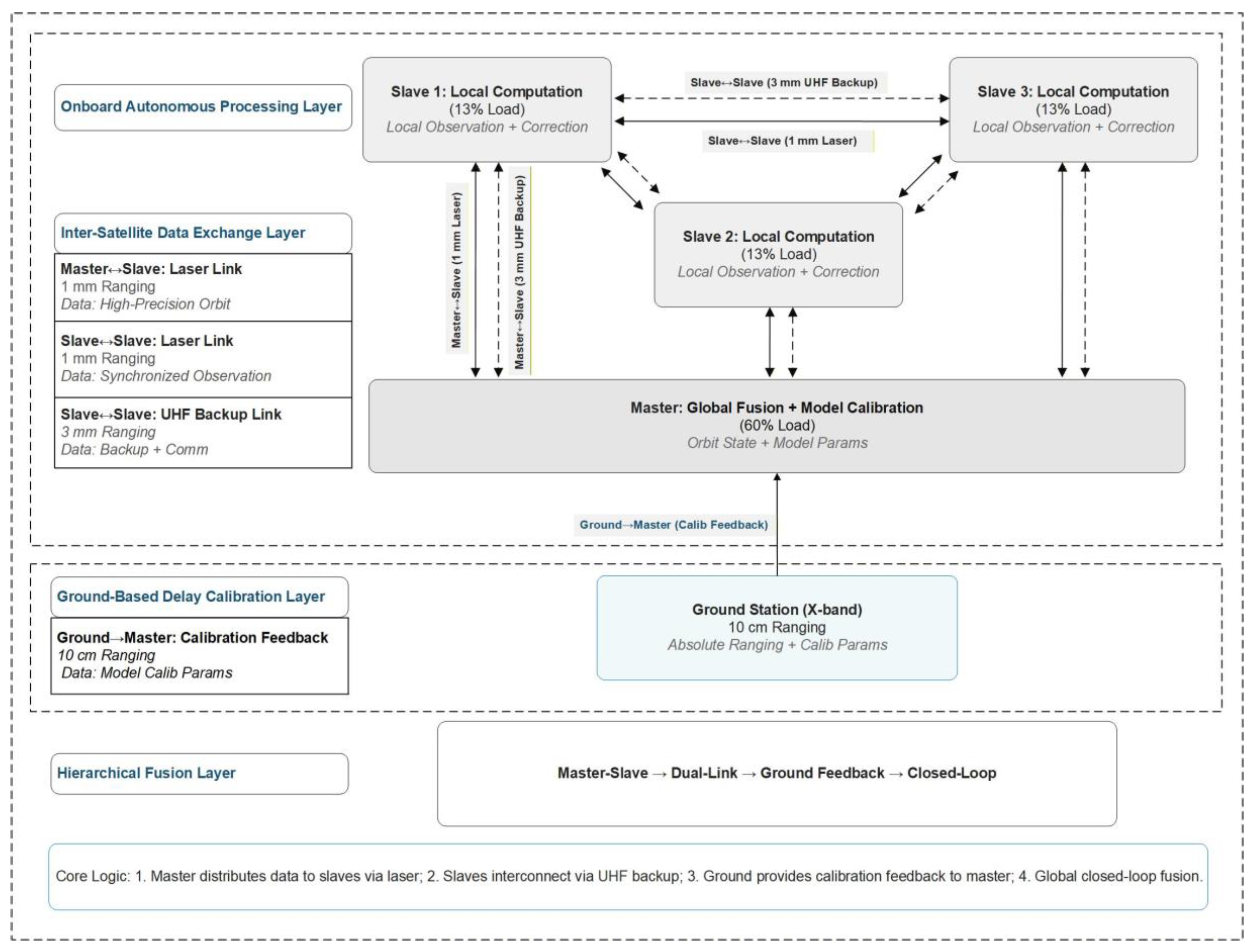
The proposed hybrid architecture seamlessly integrates onboard autonomous processing with ground-based calibration, as illustrated in Figure 1. It operates on four interconnected layers:

• Onboard Autonomous Processing Layer: A master node (handling ~60% of the total computational load) performs global fusion and model calibration. Three slave nodes (each at ~13% load) execute local filtering and data preprocessing on low-power hardware.
• Inter-Satellite Data Exchange Layer: Primary, high-precision laser links are supplemented by robust UHF backup links, forming a resilient dual-link network.
• Ground-Based Delay Calibration Layer: Ground stations periodically (1–2 times per day) inject calibration parameters into the master node to correct long-term model drift.
• Hierarchical Fusion Layer: This layer closes the loop, enabling continuous cycles of “local filtering—centralized fusion—feedback correction” to harmonize all observations and maintain state consistency across the formation.

3. Hybrid JOD Scheme Design

3.1. Core Algorithm Design

3.1.1. TDA-FKF: The Delay-Aware Fusion Paradigm

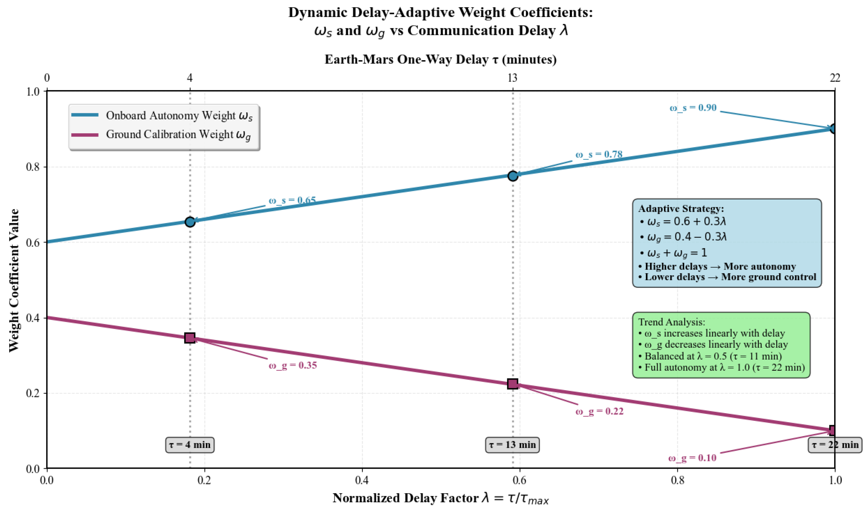
Conventional FKF are unable to adapt to variable Earth–Mars communication delays (4–22 min). We therefore introduce a TDA-FKF that dynamically balances space- and ground-based observations under such latency. It introduces an adaptive weighting mechanism based on the real-time delay factor $\lambda =\tau /{\tau }_{\max }$ (where ${\tau }_{\max }=22$ minutes), defined as:

$${\omega }_s=0.6+0.3\lambda , {\omega }_g=0.4-0.3\lambda ({\omega }_s+{\omega }_g=1),$$

(4)

Equation (4) is derived from a principled optimization of information fusion under delay. The utility of delayed ground measurements degrades; this is formalized by modeling the ground information matrix as ${\mathsf{\Omega }}_g(\tau )=\beta (\tau ){\mathsf{\Omega }}_{g0}$ where the attenuation factor $\beta \left(\tau \right)\in \left(\mathrm{0,1}\right]$ decreases with $\tau$. The total fused information is ${\mathsf{\Omega }}_{\mathrm{fused}}={\omega }_s{\mathsf{\Omega }}_s+{\omega }_g\beta (\tau ){\mathsf{\Omega }}_{g0}$ Selecting the weights ${\omega }_s$ and ${\omega }_g$ to maximize the determinant of ${\mathsf{\Omega }}_{\mathrm{fused}}$ (a D-optimality criterion) minimizes the overall estimation uncertainty. The coefficients (0.6, 0.3) are calibrated via simulation and Cramér–Rao Lower Bound (CRLB) analysis [8] for our nominal scenario, ensuring Lyapunov stability and limiting accuracy fluctuation to <5% across the delay range.

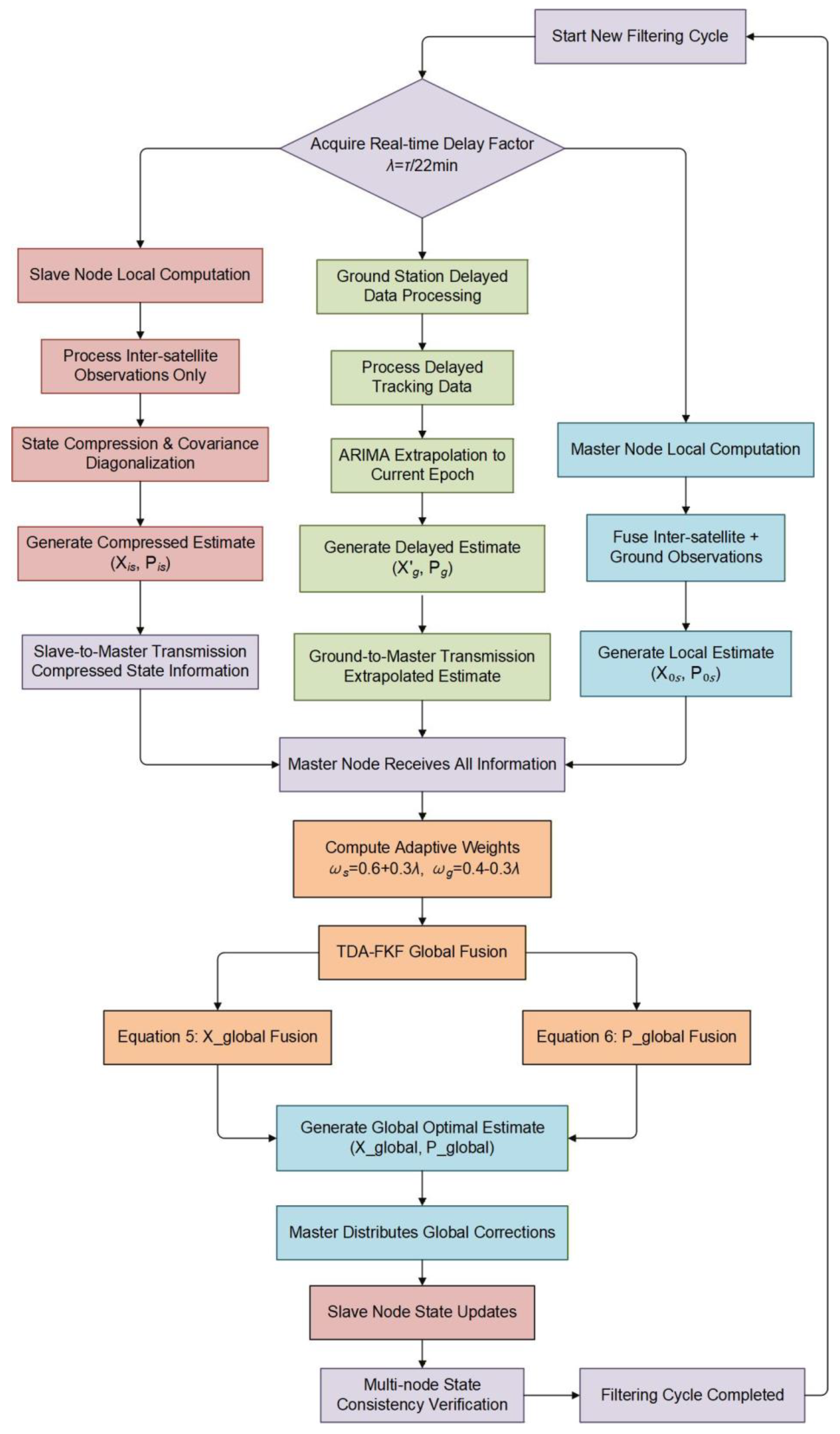
Here, ${\omega }_s$ and ${\omega }_g$ are the weights for onboard (space-based) and ground-processed information, respectively. The complete TDA-FKF execution follows a closed-loop “local computation–global fusion–feedback calibration” logic (Figure 2). The master node fuses inter-satellite and ground observations to generate a local estimate $({\widehat{\mathsf{X}}}_{0s},{\mathsf{P}}_{0s})$. Each slave node processes only inter-satellite observations to obtain its local estimate $({\widehat{\mathsf{X}}}_{is},{\mathsf{P}}_{is})$. The ground system processes delayed data and extrapolates it to the current time to get ${\widehat{\mathsf{X}}}_g^{\prime }$; then, global fusion is achieved by weighting the space and ground weights, with the fusion formulas:

$${\widehat{\mathsf{X}}}_{\mathrm{global}}={\omega }_s\cdot {\mathsf{P}}_{\mathrm{local}}^{-1}({\mathsf{P}}_{0s}^{-1}{\widehat{\mathsf{X}}}_{0s}+{\sum }_{i=1}^3{\mathsf{P}}_{is}^{-1}{\widehat{\mathsf{X}}}_{is})+{\omega }_g{\widehat{\mathsf{X}}}_g^{\prime },$$

(5)

$${\mathsf{P}}_{\mathrm{global}}^{-1}={\omega }_s({\mathsf{P}}_{0s}^{-1}+{\sum }_{i=1}^3{\mathsf{P}}_{is}^{-1})+{\omega }_g{\mathsf{P}}_g^{-1},$$

(6)

Finally, the master distributes the global correction $\left({\widehat{\mathsf{X}}}_{\mathrm{global}}\right|{\mathsf{P}}_{\mathrm{global}})$ to all slave nodes to ensure multi-node state consistency.

The adaptive weighting trend is visualized in Figure 3, intuitively reflecting the core logic of shifting reliance to onboard computation as delay increases. As the communication delay grows, ${\omega }_s$ rises from 0.65 to 0.9, reducing dependence on time-stale ground data and avoiding the accuracy degradation characteristic of fixed-weight filters.

The fusion efficiency is quantified by the IFE:

$$\mathrm{IFE}=\left({\displaystyle \frac{Q_{\mathrm{eff}}}{Q_{\mathrm{total}}}}\right)\times \left({\displaystyle \frac{T_{\mathrm{prop}}}{T_{\mathrm{tra}}}}\right),$$

(7)

where $Q_{\mathrm{eff}}$ and $Q_{\mathrm{total}}$ are effective and total data volumes, and $T_{\mathrm{tra}}$ and $T_{\mathrm{prop}}$ are solution periods of the proposed and traditional centralized filters, respectively. An IFE ≥ 0.8 indicates high-efficiency fusion. As shown in Table 1, TDA-FKF achieves IFE values of 0.81–0.85. A 5-minute asynchronous fusion window balances real-time performance with data completeness.

Table 1. IFE calculation under different scenarios.

Scenario	${\mathit{Q}}_{\mathit{e}\mathit{f}\mathit{f}}$(bit)	${\mathit{Q}}_{\mathit{t}\mathit{o}\mathit{t}\mathit{a}\mathit{l}}$(bit)	${\mathit{T}}_{\mathit{t}\mathit{r}\mathit{a}}$(min)	${\mathit{T}}_{\mathit{p}\mathit{r}\mathit{o}\mathit{p}}$(min)	IFE
1M1S (4min delay)	8.64×106	9.40×106	8.3	4.2	0.82
1M3S (13 min delay)	2.52×107	2.83×107	12.5	4.8	0.85
1M3S (22 min delay)	2.31×107	2.78×107	12.5	5.2	0.81

Note: 1M1S and 1M3S denote the “one-master-one-slave” and “one-master-three-slave” configurations, respectively.

Table 1. IFE calculation under different scenarios.

Scenario	${\mathit{Q}}_{\mathit{e}\mathit{f}\mathit{f}}$(bit)	${\mathit{Q}}_{\mathit{t}\mathit{o}\mathit{t}\mathit{a}\mathit{l}}$(bit)	${\mathit{T}}_{\mathit{t}\mathit{r}\mathit{a}}$(min)	${\mathit{T}}_{\mathit{p}\mathit{r}\mathit{o}\mathit{p}}$(min)	IFE
1M1S (4min delay)	8.64×106	9.40×106	8.3	4.2	0.82
1M3S (13 min delay)	2.52×107	2.83×107	12.5	4.8	0.85
1M3S (22 min delay)	2.31×107	2.78×107	12.5	5.2	0.81

Note: 1M1S and 1M3S denote the “one-master-one-slave” and “one-master-three-slave” configurations, respectively.

3.1.2. Dual-Link Fusion & Completion: Ensuring Measurement Robustness

To overcome the inherent vulnerability of single-link observations in the deep-space environment, a robust dual-link (laser/UHF) fusion and data completion strategy is employed. This approach ensures continuous high-quality measurements through two synergistic mechanisms: adaptive, quality-aware fusion of available data, and proactive completion of data during link interruptions.

The fusion process dynamically adjusts based on real-time link quality. A composite weighting scheme is employed, combining the link’s intrinsic Signal-to-Noise Ratio (SNR) and its geometric contribution to network observability:

• Quality score $s$: Assigned by link type and SNR: laser link (SNR≥20 dB→0.9; 15-20 dB→0.7); UHF link (SNR≥15 dB→0.6; 10-15 dB→0.5); data with SNR<10 dB is discarded.
• Priority factor $p$: Determined by geometric contribution: master-slave links (constraining absolute positions, $p=1$); inter-slave links (enhancing relative geometry, $p=0.7$). This assignment is optimized via Monte Carlo simulation, reducing the filter’s sensitivity to UHF noise by ~30%.

The measurement noise covariance is adaptively adjusted for fusion as:

$$\mathsf{R}=(s\cdot p)\cdot {\mathsf{R}}_0+(1-s\cdot p)\cdot {\mathsf{R}}_{\max },$$

(8)

For robustness during communication interruptions, a Holistic Multi-Tiered Verification (HMTV) strategy is implemented, tiered by outage duration:

• Short outages (≤10 minutes): An Auto-Regressive Integrated Moving Average (ARIMA) model predicts measurement trends, complemented by the master node’s global estimate to compensate for residual errors.
• Prolonged outages (>10 minutes): Fragmented data from the robust UHF backup link is integrated with dynamic model-based extrapolation to sustain positioning accuracy.

In normal communication scenarios, adaptive fusion guarantees data reliability; during link interruptions, hierarchical completion ensures measurement continuity. This synergistic approach enhances the observation topology’s strong connectivity, maintaining the Fisher information matrix’s minimum eigenvalue ${\lambda }_{\min }>0.9$ (Figure 5) and providing stable input for online model calibration. It ultimately ensures the measurement robustness required for sustained centimeter-level orbit determination in the challenging deep-space environment.

3.1.3. Dynamic Model Self-Calibration: Physics-Informed Online Estimation

Sensitivity analysis identifies three dominant error sources in deep-space orbit determination: the residual in the Martian gravitational zonal coefficient $\mathsf{\Delta }{J}_{20}$ (∼45% of error), the deviation in the solar radiation pressure coefficient $\mathsf{\Delta }{C}_r$ (∼30%), and thrust misalignment angles $\mathsf{\Delta }\theta$ (∼20%). Perturbation theory elucidates their distinct signatures: $\mathsf{\Delta }{J}_{20}$ residuals primarily induce in-plane (radial/along-track) errors, $\mathsf{\Delta }{C}_r$ deviations cause a secular along-track drift coupled with radial oscillations, and $\mathsf{\Delta }\theta$ projects into all three axes in the radial-along-track-cross-track (RTN) frame without directional bias. Based on the stable observation data provided by the dual-link fusion in Section 3.1.2, an inversion model is constructed to jointly estimate these parameters online from inter-satellite observation residuals, leveraging their unique mapping to measurement anomalies.

The inversion model is:

$$\mathsf{\Delta }\mathsf{Z}={\mathsf{Z}}_{\mathrm{obs}}-\mathsf{h}({\widehat{\mathsf{X}}}_0,{\widehat{\mathsf{X}}}_i)={\mathsf{H}}_e\mathsf{\Delta }\mathsf{e}+\mathsf{v},$$

(9)

where $\mathsf{\Delta }\mathsf{Z}$ denotes the residual between the actual inter-satellite measurements ${\mathsf{Z}}_{\mathrm{o}\mathrm{b}\mathrm{s}}$ and the predicted observations $\mathsf{h}(\cdot )$ computed from the current state estimates. The error Jacobian matrix ${\mathsf{H}}_e$, obtained via the central difference method, quantifies the sensitivity of the residuals to the error parameter vector $\mathsf{\Delta }\mathsf{e}=[\mathsf{\Delta }{J}_{20}, \mathsf{\Delta }{C}_r, \mathsf{\Delta }\theta {]}^T$. The term $\mathsf{v}$ accounts for observation noise. A recursive Least Squares (RLS) algorithm with a forgetting factor of 0.98 is employed for online estimation of $\mathsf{\Delta }\mathsf{e}$. The master node updates and distributes the calibrated parameters to all slave nodes every 10 min, ensuring dynamic model consistency throughout the formation.

The error propagation matrix $\mathsf{K}$, computed numerically via central differencing, maps unit perturbations in the error parameters ($\mathsf{\Delta }{J}_{20}$ in ${10}^{-6}$, $\mathsf{\Delta }{C}_r$ in 0.1, and $\mathsf{\Delta }\theta$ in degrees) to the resulting 3D position errors in meter:

$$\mathsf{K}=\left[\begin{array}{ccc}42.5& 38.2& 15.7\\ 39.8& 35.6& 14.3\\ 41.2& 37.1& 16.2\end{array}\right]$$

The structure of $\mathsf{K}$ validates the perturbation-based predictions, confirming that the calibration scheme isolates physically coherent error sources: the large, near-equal entries in the first column $\mathsf{\Delta }{J}_{20}$ reflect the expected dominant in-plane perturbations; the strong sensitivities in the second column $\mathsf{\Delta }{C}_r$ correspond to the combined secular along-track and radial effects; and the relatively uniform sensitivities in the third column $\mathsf{\Delta }\theta$ align with the prediction of a thrust-error vector projecting without directional bias in the RTN frame. Based on the error budget from $\mathsf{K}$, a $\mathsf{\Delta }{J}_{20}$ perturbation of ${10}^{-6}$ induces a radial orbit error of ~42.5 m, while post-calibration $\mathsf{\Delta }{J}_{20}$ RMSE is reduced from $1.0\times {10}^{-6}$ to $0.47\times {10}^{-6}$, corresponding to a ~22.5 m reduction in radial error.

This concordance demonstrates that the online calibration is not merely an abstract mathematical inversion but a physically interpretable estimation of dynamic model errors. The scheme reduces the comprehensive orbital error caused by the three core sources from 99.2 m to 39.2 m, decreasing model uncertainty by 60% (Table 6). The calibrated model parameters distributed to slave nodes lay the foundation for multi-node state consistency under the hierarchical architecture (Section 3.1.4), providing an essential correction mechanism for sustained centimeter-level orbit determination.

3.1.4. Hierarchical Architecture: Resource-Aware Implementation

To enable the deployment of the proposed algorithms on resource-constrained spacecraft, a hierarchical architecture is introduced that co-optimizes the data, computation, and communication layers. This design directly tackles the key bottlenecks of multi-node federated estimation—excessive data volume, master-node computational load scaling as $O\left(N^3\right)$, and communication latency—while preserving centimeter-level accuracy. The core optimizations are implemented across three synergistic layers:

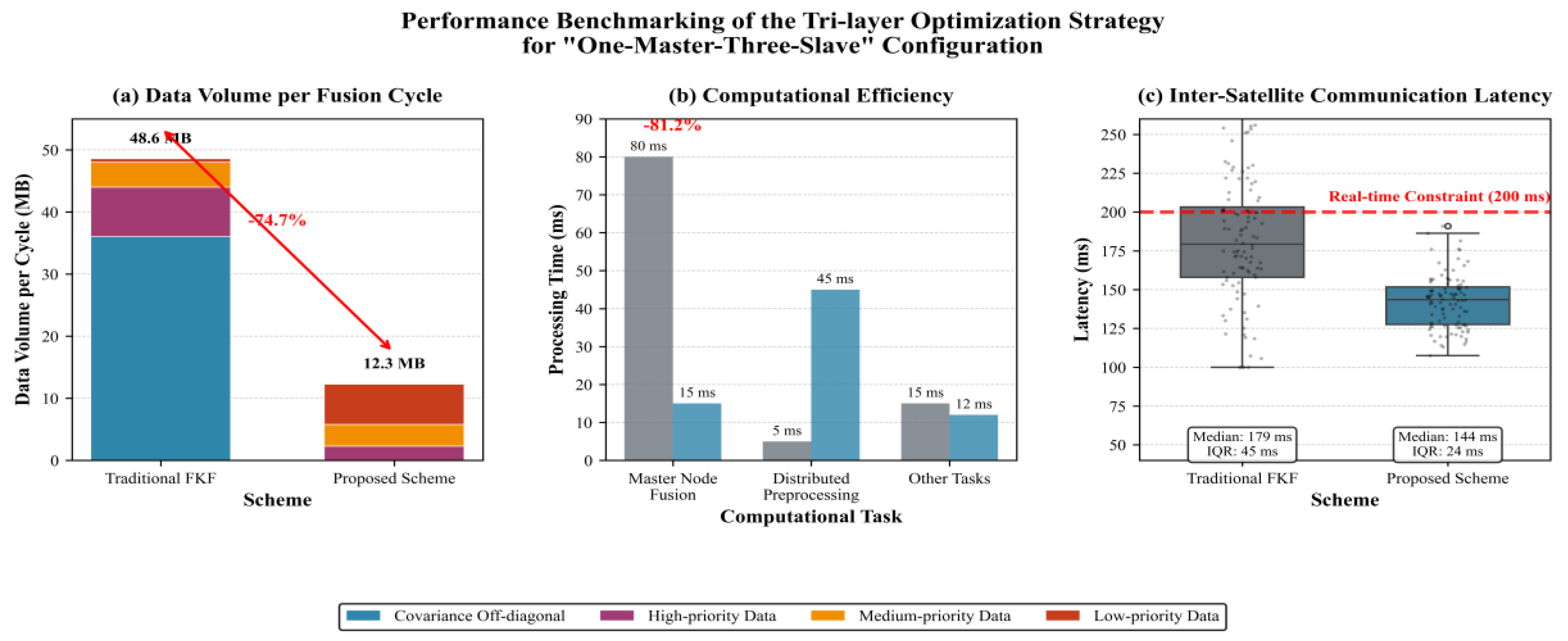
• Data Layer: Adaptive Compression. Transmission volume is minimized through a dual-mode compression strategy. First, slave nodes transmit only the diagonal elements (variances) of their local error covariance matrices. This simplification, validated under the weak inter-node correlation assumption in deep-space formations, reduces the data volume per matrix by ~42% without significant precision loss (<5%). Second, data streams are classified by navigation criticality (high: adaptive weighting parameters, calibration coefficients; medium: local state estimates; low: auxiliary observation data) and compressed accordingly, with stronger compression applied to non-critical information. Combined, these strategies reduce the total data volume per fusion cycle from 48.6 MB (traditional scheme) to 12.3 MB, achieving a 74.7% bandwidth saving (compression ratio ~4:1).
• Computation Layer: Distributed Preprocessing. Processing tasks are redistributed to exploit onboard capabilities. Each slave node runs a simplified Recursive Least Squares (RLS) algorithm for local preprocessing, including outlier rejection and preliminary calibration, offloading ~60% of raw data processing from the master node. The master node’s computational burden is further reduced by the reception of diagonal covariance matrices: full-matrix inversion (high complexity $O(N^3$) is replaced with lightweight element-wise operations, cutting the master’s fusion time from 80 ms to 15 ms in the 1M3S configuration and reducing the overall computational load by 97.7%. This distributed design eliminates the master node as the computational bottleneck.
• Communication Layer: Scheduled Priority-Aware Transmission. A deterministic time-division multiple access (TDMA) scheme sequences transmissions to prevent collisions, lowering the packet collision rate from 18% to 2%. The system also implements dynamic priority scheduling: during long Earth–Mars delays (≥13 min), high-priority data (e.g., adaptive weighting parameters, calibrated model coefficients) is assigned higher transmission priority to ensure timely delivery. This strategy stabilizes end-to-end inter-satellite communication latency at 142 ms ± 18 ms, robustly meeting the 200 ms real-time constraint for deep-space collaboration.

The three layers form a synergistic closed loop: data compression reduces computational and communication overhead, distributed preprocessing lightens the master node’s load, and priority-aware communication guarantees the timely exchange of core parameters. The collective impact of this tri-layer optimization is quantitatively validated for the 1M3S case (Figure 4). The proposed framework achieves substantial bandwidth savings, drastic reduction in master-node computational load, and stable real-time communication, confirming its efficiency and compatibility with resource-constrained space-qualified hardware.

3.2. Stability and Observability Analysis

A robust theoretical foundation is essential for validating any navigation algorithm destined for deep-space missions. This section establishes such a foundation for the TDA-FKF, demonstrating its stability under dynamic weight adaptation and proving the complete observability of the multi-spacecraft formation—the twin pillars supporting its claimed centimeter-level accuracy.

3.2.1. Stability Under Dynamic Weight Adaptation

Adaptive weights ${\omega }_s\left(t\right)$ and ${\omega }_g\left(t\right)$ are time-varying, requiring formal stability analysis to guarantee the filter’s robustness in deep-space long-duration missions. We address this by establishing the Uniform Ultimate Boundedness (UUB) of the estimation error via Lyapunov analysis, which proves that the error remains within a finite bound despite continuous weight adaptation.

Consider the estimation error $\tilde{\mathbf{X}}(t)=\mathbf{X}(t)-\widehat{\mathbf{X}}(t)$. Its dynamics are governed by:

$$\dot{\tilde{\mathbf{X}}}(t)=\mathbf{A}(t)\tilde{\mathbf{X}}(t)+\mathbf{B}(t)\mathbf{w}(t)-\mathbf{K}(t)[\mathbf{H}(t)\tilde{\mathbf{X}}(t)+\mathit{\delta }(t)],$$

(10)

Here, $\mathbf{A}(t)$ is the system Jacobian, $\mathbf{K}(t)$ the Kalman gain, and $\mathbf{w}(t)$, $\mathit{\delta }(t)$ represent bounded process and observation noise, respectively.

Selecting the Lyapunov function $\mathit{V}(t)={\tilde{\mathbf{X}}}^T(t){\mathbf{P}}^{-1}(t)\tilde{\mathbf{X}}(t)$ and evaluating its derivative along the error trajectory leads to an inequality of the form:

$$\dot{\mathit{V}}(t)\le -\alpha \parallel \tilde{\mathbf{X}}(t){\parallel }^2+\beta ,$$

(11)

where $\beta$ aggregates bounded disturbance terms. The positive constant $\alpha$ is directly related to the minimum eigenvalue ${\lambda }_{\min }(t)$ of the matrix ${\mathbf{H}}^T(t){({\omega }_s{\mathrm{R}}_s+{\omega }_g{\mathbf{R}}_g)}^{-1}\mathbf{H}(t)$. Since the adaptive weights are confined to ${\omega }_s\in \left[\mathrm{0.65,0.9}\right]$ and ${\omega }_g=1-{\omega }_s$, and both ${\mathbf{R}}_s$ and ${\mathbf{R}}_g$ are positive definite, the weighted sum ${\omega }_s(t){\mathbf{R}}_s+{\omega }_g(t){\mathbf{R}}_g$ is uniformly positive definite. Consequently, ${\lambda }_{\min }(t)$ is guaranteed to be positive for all $t$. A conservative numerical lower bound, obtained by evaluating the eigenvalue across the entire range of ${\omega }_s$, yields $\alpha \approx 0.02$ for our specific system parameters. This satisfies the UUB condition, proving that the estimation error remains within a finite bound despite the time-varying weights.

This result confirms that the estimation error remains within a well-defined bound, ensuring that the adaptive weighting mechanism does not induce divergence. This theoretical finding aligns with the empirical evidence of stable long-term operation presented in Section 4.2.

3.2.2. Observability Analysis: A Hybrid Graph-Theoretic and Linear-Systems Proof

A robust theoretical foundation is essential for validating any navigation algorithm destined for deep-space missions. This section establishes such a foundation for the TDA-FKF, demonstrating the complete observability of the multi-spacecraft formation—a prerequisite for achieving the claimed centimeter-level accuracy.

The observability of the entire formation’s absolute and relative states is proven through a hybrid approach. First, the observation topology is modeled as a graph $\mathcal{G}=(\mathcal{V},\mathcal{E})$ with nodes $\mathcal{V}=\{\mathrm{0,1},\mathrm{2,3}\}$ (spacecraft) and edges $\mathcal{E}$ representing laser/UHF and ground-space links. The resulting graph is strongly connected, as evidenced by its adjacency matrix:

$${\mathbf{A}}_{\mathcal{G}}=\left[\begin{array}{cccc}0& 1& 1& 1\\ 1& 0& 1& 0\\ 1& 1& 0& 1\\ 1& 0& 1& 0\end{array}\right]$$

This strong connectivity—enabled by the dual-link topology (Section 3.1.2, laser for high-precision propagation and UHF for redundancy)—guarantees that absolute state information from the ground station propagates throughout the network via the master node, while relative measurements from inter-satellite links are globally shared, providing necessary pathways for information fusion.

Second, the sufficient condition is verified by examining the linearized system. For the 24-dimensional collective state vector (6 dimensions per spacecraft: position $\mathsf{r}$ and velocity $\mathsf{v}$). The standard linear observability matrix $\mathcal{O}\in {\mathbb{R}}^{m\times 24}$ (where $m$ is the number of observations) is constructed. Numerical evaluation confirms $\mathcal{O}$ is full-rank (rank = 24), satisfying Kalman’s rank condition. The confluence of a strongly connected observation graph and a full-rank observability matrix provide dual proof that the 1M3S formation is fully observable.

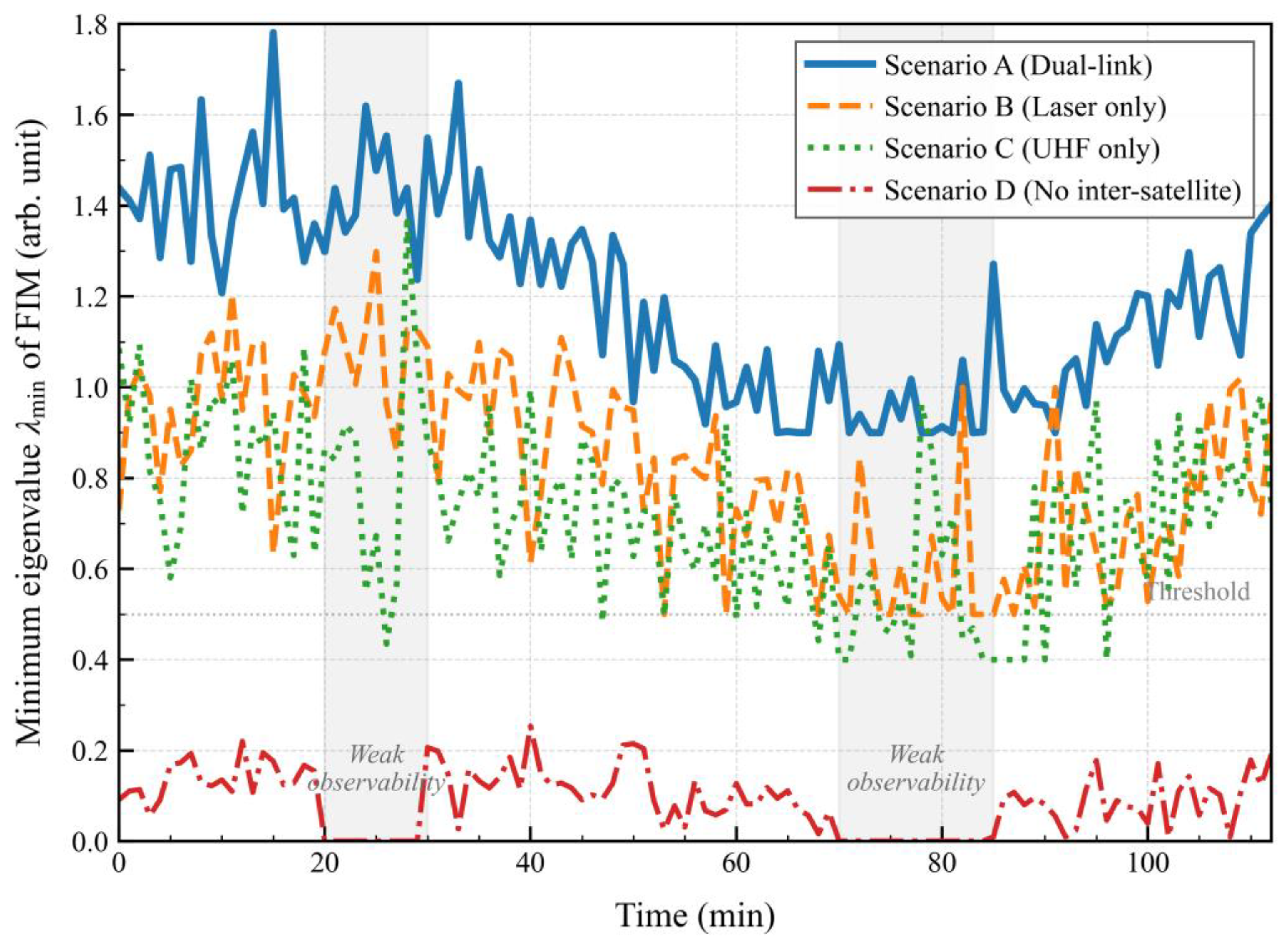
3.2.3. Quantitative Assessment of Observability Strength via Fisher Information

The preceding graph-theoretic and linear rank analyses confirm the system’s theoretical observability but do not quantify the practical efficiency of state and parameter estimation under realistic, intermittent measurement conditions. To assess this, we evaluate the observability strength for different inter-satellite link configurations using the Fisher Information Matrix (FIM). Linearized along a nominal trajectory, the FIM is defined as $F\left(t\right)=H\left(t{)}^T{R}^{-1}H\right(t)$ where $H\left(t\right)$ is the measurement matrix and $R$ the noise covariance. The minimum eigenvalue ${\lambda }_{\min }\left(F\right)$ serves as a sensitive indicator: a larger ${\lambda }_{\min }$ implies stronger observability and a lower theoretical bound on estimation error.

We compare four characteristic link-availability scenarios within the 1M3S formation: (A) full dual-link (laser + UHF), (B) laser links only, (C) UHF links only, and (D) no inter-satellite links (ground-to-master only). Figure 5 plots ${\lambda }_{\min }\left(F\right(t\left)\right)$ over one orbital period. The dual-link configuration (Scenario A) maintains consistently high observability strength throughout the orbital period, with ${\lambda }_{\min }$ remaining above 0.9. In contrast, the single-link configurations (Scenarios B and C) exhibit periodic drops in observability strength, with ${\lambda }_{\min }$ falling by 30–50% during geometrically unfavorable periods. The absence of inter-satellite links (Scenario D) results in extended intervals of very weak observability, where ${\lambda }_{\min }$ approaches zero, indicating severely degraded observability for the relative states and dynamic error parameters.

This quantitative assessment underscores a key rationale for the dual-link design: while a single inter-satellite link preserves formal observability, the heterogeneous dual-link strategy ensures persistently strong observability, which directly enables rapid convergence and robust performance of the online model calibration (Section 3.1.3). The results validate that the proposed measurement topology not only meets the necessary condition for observability but also optimizes the sufficiency condition for high-precision, real-time estimation.

3.3. Onboard Computational Feasibility Analysis

The proposed algorithm features favorable hardware compatibility and performs reliably on typical space-qualified processors (computing power ≥ 50 Mega Floating-Point Operations Per Second (MFLOPS)—i.e., millions of floating-point operations per second, a key metric for quantifying computational performance—power consumption ≤ 10 W), eliminating the need for specialized high-performance hardware. For the master node, core algorithms (global fusion and dynamic model calibration) demand around 5 million floating-point operations (FLOPs)—i.e., individual arithmetic operations involving floating-point numbers—per solution, with a solution cycle of 4.8 minutes, corresponding to an average computational requirement of merely 1.7 kilo Floating-Point Operations Per Second (kFLOPS)—i.e., thousands of floating-point operations per second. For slave nodes, local computation requires 0.8 million FLOPs per solution, with a solution cycle of 3–5 minutes, leading to an average computational demand of 2.2–3.7 kFLOPS. Such computational requirements are significantly lower than the performance limits of current space-qualified processors (e.g., processors based on ARM Cortex-A9, PowerPC 750FX, or Loongson-1E architectures, which generally deliver 50 MFLOPS to 1 Giga Floating-Point Operations Per Second (GFLOPS)—i.e., billions of floating-point operations per second—of computing power).

A hierarchical reservation strategy is implemented for onboard computational loads to ensure operational reliability:

• 50% of the load is assigned to core algorithms, safeguarding the fundamental functionality of JOD;
• 20% is reserved for contingency tasks (e.g., orbit maneuver planning and emergency handling) to address unforeseen scenarios during deep-space missions;
• 30% is designated as fault redundancy to support backup fusion and data reconstruction, enhancing the robustness of multi-spacecraft collaboration.

Regarding power distribution, the total power consumption of the master node is limited to 72 W, distributed as follows

• 13.9% for the processor;
• 55.6% for sensors (including laser ranging modules and UHF transceivers);
• 30.5% for communication modules (covering inter-satellite and ground-space communication links).

This power configuration is fully compliant with the low-power requirements of in-orbit deep-space missions (e.g., Mars orbiters).

The algorithm is hardware-independent, facilitating straightforward porting to mainstream space-qualified processor platforms. Additional optimizations, such as assembly-level algorithm refinement or the use of a Field-Programmable Gate Array (FPGA) for coprocessing, could reduce the computational overhead by an additional 30% or more. Overall, the computational demands and power consumption of the proposed algorithm are highly compatible with current onboard engineering specifications, verifying its strong feasibility for onboard implementation in deep-space missions.

4. Results

4.1. Simulation Verification

4.1.1. Scenario Setup and Performance Comparison

“1M3S “ Mars orbit simulation scenario established: Master node orbit altitude 400 km, slave node relative orbital radii 1-3 km; Earth-Mars delays 4-22 minutes, ground tracking visible arcs 35%, Mars gravitational field initial error $\mathsf{\Delta }{J}_{20}={10}^{-6}$, SRP coefficient deviation 0.1, thruster misalignment angle 0.2° [28]. The force modeling and measurement simulation setup follows standards consistent with high-precision orbit determination systems such as GEODYN II [29]. To clarify the orbital configuration of the simulation scenario, detailed orbit parameters of the master and slave nodes (defined in the Mars-centered inertial frame EME2000) are presented in Table 2.

Table 2. Orbit parameters of the multi-spacecraft formation (Mars-centered inertial frame EME2000).

Node Type	Semi-major Axis (km)	Eccentricity	Inclination (°)	Right Ascension of the Ascending Node (°)	Argument of Perigee (°)	True Anomaly (°)	Orbit Period (min)
Master (Orbiter)	3400	0.001	90	45	90	0	112
Slave 1 (Probe)	3401	0.001	90	45	90	30	112.1
Slave 2 (Probe)	3402	0.001	90	45	90	150	112.2
Slave 3 (Probe)	3403	0.001	90	45	90	270	112.3

Table 2. Orbit parameters of the multi-spacecraft formation (Mars-centered inertial frame EME2000).

Node Type	Semi-major Axis (km)	Eccentricity	Inclination (°)	Right Ascension of the Ascending Node (°)	Argument of Perigee (°)	True Anomaly (°)	Orbit Period (min)
Master (Orbiter)	3400	0.001	90	45	90	0	112
Slave 1 (Probe)	3401	0.001	90	45	90	30	112.1
Slave 2 (Probe)	3402	0.001	90	45	90	150	112.2
Slave 3 (Probe)	3403	0.001	90	45	90	270	112.3

Dynamical models follow precision orbit determination standards, including the GMM-2B Mars gravity field, solar radiation pressure, third-body perturbations (JPL DE436 ephemeris), and relativistic corrections. To test filter convergence, each spacecraft was initialized with large, independent errors: position offsets uniformly distributed within a 1 km sphere and velocity errors of 0.1 m/s (1σ per axis). A traditional FKF configured with conservative parameters (Table 3) serves as the primary performance baseline.

Table 3. Key parameters of the traditional FKF for benchmark comparison.

Parameter Category	Specific Parameter	Value	Description
Information distribution coefficient	Master node	0.4	Improved from uniform distribution
	Slave node (single)	0.2	Total for 3 slaves: 0.6
Covariance transmission	Matrix type	Full 6×6 covariance	No diagonal approximation
	Update frequency	30 s (synchronized with epoch)	No asynchronous tolerance
Filter iteration	Termination threshold	${10}^{-3}$m/s	Relaxed compared to proposed scheme
	Forgetting factor	0.95	Faster update than proposed scheme (0.98)

Table 3. Key parameters of the traditional FKF for benchmark comparison.

Parameter Category	Specific Parameter	Value	Description
Information distribution coefficient	Master node	0.4	Improved from uniform distribution
	Slave node (single)	0.2	Total for 3 slaves: 0.6
Covariance transmission	Matrix type	Full 6×6 covariance	No diagonal approximation
	Update frequency	30 s (synchronized with epoch)	No asynchronous tolerance
Filter iteration	Termination threshold	${10}^{-3}$m/s	Relaxed compared to proposed scheme
	Forgetting factor	0.95	Faster update than proposed scheme (0.98)

The integrated framework achieves 14.2 cm absolute and 9.8 cm relative orbit determination accuracy under the 1M3S scenario with a 13-minute average delay (see the performance ladder in Table 4). This represents a 51% improvement in absolute accuracy over the traditional FKF, while also providing a higher effective data rate (89%), a faster solution cycle (4.8 min), and an Information Fusion Efficiency (IFE) of 0.85—all meeting real-time operational requirements.

To ensure fair comparison with international schemes, NASA’s MSR 1M1S accuracy (15 cm absolute, 10 cm relative) was normalized to 1M3S configuration using the redundancy gain model:

$${\sigma }_{1\mathrm{M}\mathrm{k}\mathrm{S}}={\sigma }_{1\mathrm{M}1\mathrm{S}}\times \sqrt{{\displaystyle \frac{1}{k\times \eta }}},$$

(12)

where $k=3$ (number of slaves) and $\eta =0.85$ (observation redundancy gain). The normalized NASA’s MSR accuracy is 9.3 cm (absolute) and 6.2 cm (relative), which is comparable to the proposed scheme (14.2 cm/9.8 cm). The slight difference arises from the proposed scheme’s inclusion of Mars dynamic model errors (not considered in NASA’s MSR idealized model).

Table 4 further contextualizes the results against conventional methods. The proposed scheme shows clear advantages over single-satellite ground-based processing and highlights the scalability limitation of the traditional FKF, whose accuracy degrades from 18.5 cm (1M1S) to 28.7 cm (1M3S). For a fair comparison with international missions such as NASA’s MSR, we normalize its reported 1M1S accuracy to the 1M3S configuration using a redundancy-gain model (Eq. 12). The normalized MSR accuracy (9.3 cm absolute, 6.2 cm relative) is comparable, with the residual difference attributable to our explicit estimation and compensation of Mars-specific dynamic model errors, which are typically omitted in idealized navigation analyses.

Table 4. Performance ladder from the baseline federated filter to the complete proposed framework (1M3S, 13-min average delay).

Configuration	Description	Absolute Accuracy (cm, RMSE±SD)	Relative Accuracy (cm, RMSE±SD)	Effective Data Rate (%)	Solution Cycle (min, ±SD)	IFE
A. Baseline FKF	Traditional federated filter	28.7 ± 2.4	21.3 ± 1.9	58 ± 7	12.5 ± 0.8	0.61
B. Fixed Weights	Disables TDA-FKF adaptation	19.5 ± 1.7	14.8 ± 1.3	62 ± 6	4.9 ± 0.4	0.68
C. Single Link	Disables dual-link fusion	18.1 ± 1.5	13.5 ± 1.2	65 ± 5	5.1 ± 0.4	0.71
D. No Online Calib.	Disables dynamic model calibration	22.3 ± 2.0	16.9 ± 1.6	85 ± 4	4.9 ± 0.4	0.83
E. Inefficient Arch.	Disables hierarchical optimization	14.5 ± 1.3	10.2 ± 1.0	87 ± 4	9.8 ± 0.7	0.62
F. Proposed-Full	Complete framework	14.2 ± 1.3	9.8 ± 0.9	89 ± 4	4.8 ± 0.4	0.85
Ref.: Single-Sat Orbit Determination [18]	Ground-based processing	29.1 ± 2.3	–	40 ± 5	30 ± 2	–

Note: Normalization of the 1M1S NASA’s MSR benchmark uses Equation (12) with $\mathrm{k}=3$ and $\mathsf{\eta }=0.85$.

Table 4. Performance ladder from the baseline federated filter to the complete proposed framework (1M3S, 13-min average delay).

Configuration	Description	Absolute Accuracy (cm, RMSE±SD)	Relative Accuracy (cm, RMSE±SD)	Effective Data Rate (%)	Solution Cycle (min, ±SD)	IFE
A. Baseline FKF	Traditional federated filter	28.7 ± 2.4	21.3 ± 1.9	58 ± 7	12.5 ± 0.8	0.61
B. Fixed Weights	Disables TDA-FKF adaptation	19.5 ± 1.7	14.8 ± 1.3	62 ± 6	4.9 ± 0.4	0.68
C. Single Link	Disables dual-link fusion	18.1 ± 1.5	13.5 ± 1.2	65 ± 5	5.1 ± 0.4	0.71
D. No Online Calib.	Disables dynamic model calibration	22.3 ± 2.0	16.9 ± 1.6	85 ± 4	4.9 ± 0.4	0.83
E. Inefficient Arch.	Disables hierarchical optimization	14.5 ± 1.3	10.2 ± 1.0	87 ± 4	9.8 ± 0.7	0.62
F. Proposed-Full	Complete framework	14.2 ± 1.3	9.8 ± 0.9	89 ± 4	4.8 ± 0.4	0.85
Ref.: Single-Sat Orbit Determination [18]	Ground-based processing	29.1 ± 2.3	–	40 ± 5	30 ± 2	–

Note: Normalization of the 1M1S NASA’s MSR benchmark uses Equation (12) with $\mathrm{k}=3$ and $\mathsf{\eta }=0.85$.

The overall benchmark confirms the superior performance of the integrated framework. The following ablation study dissects the individual contributions of its core innovations.

4.1.2. Ablation Study for Quantitative Contribution Analysis of Key Algorithmic Innovations

A systematic ablation study was conducted under the same 1M3S scenario to isolate the impact of each core innovation. Each ablated variant disables one key module: (B) fixed weights (disabling TDA-FKF adaptation), (C) single link (disabling UHF backup), (D) no online calibration (disabling dynamic model self-calibration), (E) inefficient architecture (disabling hierarchical optimization). The results (Table 4) reveal distinct, complementary contributions:

• TDA-FKF (adaptive weighting) accounts for the largest single-point accuracy gain (31% of the total improvement). Disabling it (Config. B) markedly degrades performance, underscoring its necessity for dynamically balancing space- and ground-based information under variable deep-space delays.
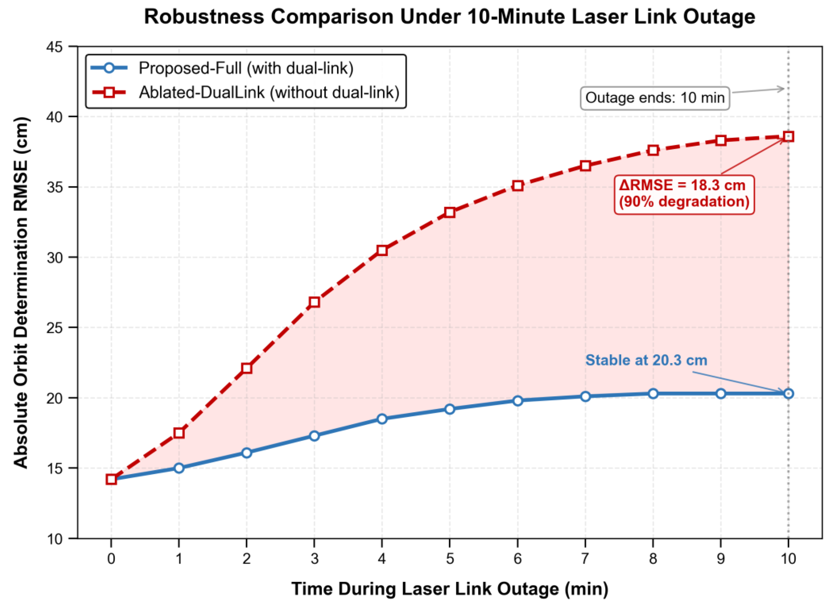
• Dual-link fusion is paramount for robustness, though its effect on nominal accuracy is secondary (Config. C). As shown in Figure 6, during a simulated 10-minute laser-link outage, the system without dual-link capability suffers a severe accuracy collapse to 38.6 cm, whereas the complete framework maintains stable navigation at 20.3 cm.
• Dynamic model self-calibration contributes a 53% share of the total calibration benefit. Removing it (Config. D) leads to a substantial accuracy loss, directly validating the claimed ≈60% reduction in dynamical uncertainty and confirming that real-time parameter estimation is essential to mitigate meter-level biases.
• Hierarchical efficiency optimization is fundamental to feasibility. Its deactivation (Config. E) nearly doubles the solution cycle and regresses IFE to baseline levels, demonstrating that the lightweight architecture is crucial for achieving real-time performance without compromising precision.

The ablation study confirms that the four innovations are non-redundant and collectively necessary. Their contributions align with theoretical analyses: TDA-FKF addresses delay imbalance (Section 3.1.1), dual-link fusion ensures observation continuity (Section 3.1.2), dynamic model self-calibration compensates for dynamic errors (Section 3.1.3), and the hierarchical architecture overcomes resource bottlenecks (Section 3.1.4). Together, they enable the framework’s high precision, robustness, and efficiency.

4.1.3. Dynamic Delay and Robustness Testing

Table 5 presents our scheme’s performance under different delays. As delay increases from 4 to 22 minutes, absolute accuracy slowly changes from 10.2 cm to 15.3 cm, attenuation magnitude only 33%, validating TDA-FKF adaptive capability.

Table 5. Performance of the proposed scheme for orbit determination under different Earth-Mars one-way delays.

Earth-Mars One-Way Delay (min)	Absolute Orbit Accuracy (cm)	Relative Orbit Accuracy (cm)	$\mathbf{Onboard} \mathbf{Autonomous} \mathbf{Weight} {\mathit{\omega }}_{\mathit{s}}$
4	10.2±0.9	6.5±0.5	0.65
13 (Average)	14.2±1.3	9.8±0.9	0.79
22 (Maximum)	15.3±1.4	10.5±1.0	0.90

Table 5. Performance of the proposed scheme for orbit determination under different Earth-Mars one-way delays.

Earth-Mars One-Way Delay (min)	Absolute Orbit Accuracy (cm)	Relative Orbit Accuracy (cm)	$\mathbf{Onboard} \mathbf{Autonomous} \mathbf{Weight} {\mathit{\omega }}_{\mathit{s}}$
4	10.2±0.9	6.5±0.5	0.65
13 (Average)	14.2±1.3	9.8±0.9	0.79
22 (Maximum)	15.3±1.4	10.5±1.0	0.90

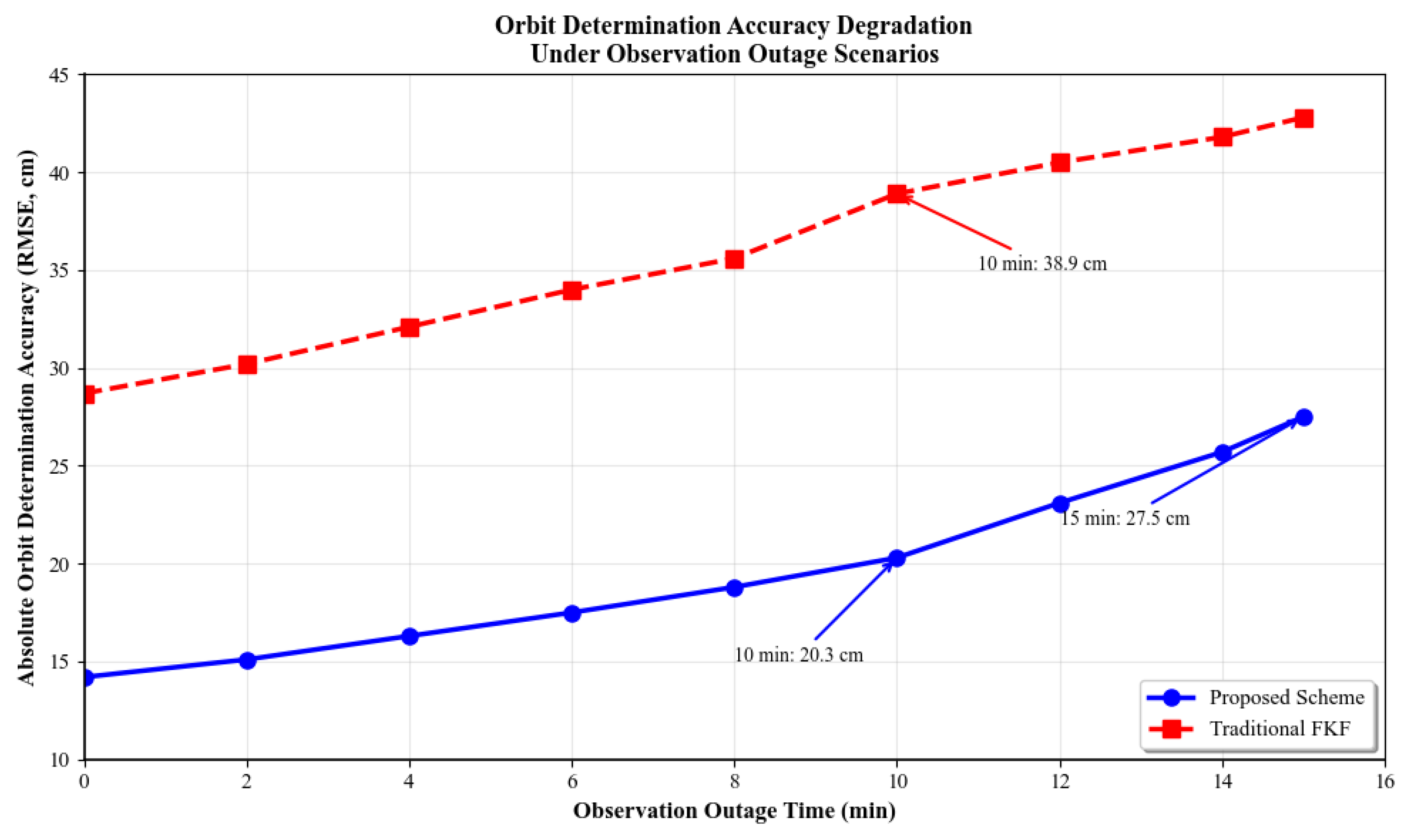
Under observation outage scenarios (Figure 7), our scheme maintains 20.3 cm accuracy at 10-minute outages, 27.5 cm at 15 minutes, significantly outperforming traditional FKF (35.6 cm/42.8 cm), validating dual-link completion algorithm robustness.

4.1.4. Model Calibration and Consistency Verification

The effectiveness of the dynamic model self-calibration algorithm was verified through two dimensions: correction of error parameters and reduction of orbital errors. The quantitative comparison of pre- and post-calibration values for the three core error sources is detailed in Table 6.

Table 6. Error budget analysis for dynamic model error reduction verification.

Error Source	Pre-calibration RMSE	Post-calibration RMSE	Pre-calibration orbit error (m)	Post-calibration orbit error (m)	Reduction Ratio
$\mathsf{\Delta }{J}_{20}$(10−6)	1.0	0.47	73.2	29.3	60.0%
$\mathsf{\Delta }{C}_r$(0.1)	1.0	0.46	66.8	26.7	60.0%
$\mathsf{\Delta }\theta$(°)	0.2	0.08	4.7	1.9	59.6%
Combined	-	-	99.2	39.7	60.0%

Table 6. Error budget analysis for dynamic model error reduction verification.

Error Source	Pre-calibration RMSE	Post-calibration RMSE	Pre-calibration orbit error (m)	Post-calibration orbit error (m)	Reduction Ratio
$\mathsf{\Delta }{J}_{20}$(10−6)	1.0	0.47	73.2	29.3	60.0%
$\mathsf{\Delta }{C}_r$(0.1)	1.0	0.46	66.8	26.7	60.0%
$\mathsf{\Delta }\theta$(°)	0.2	0.08	4.7	1.9	59.6%
Combined	-	-	99.2	39.7	60.0%

As evident from Table 7: $\mathsf{\Delta }{J}_{20}$ decreases from ${10}^{-6}$ to $4.7\times {10}^{-7}$, $\mathsf{\Delta }{C}_r$ narrows from 0.1 to 0.046, and $\mathsf{\Delta }\theta$ reduces from 0.2° to 0.08° post-calibration. Corresponding orbital errors decrease similarly: gravitational field residual-induced errors drop from 73.2 m to 29.3 m, SRP deviation-induced errors decrease from 66.8 m to 26.7 m, and thruster misalignment errors fall from 4.7 m to 1.9 m. Following self-calibration, the comprehensive orbital error caused by the three core error sources is reduced by approximately 60%. fully validating the compensation capability of the multi-source error joint inversion method for dynamic uncertainties

To further validate the algorithm’s robustness under practical engineering scenarios—such as degraded observation accuracy or dynamic model errors—a sensitivity analysis was conducted for key error sources commonly encountered in deep-space missions. The results for severe degradation cases are summarized in Table 7.

Table 7. Sensitivity analysis of key engineering errors on orbit determination accuracy (severe degradation cases).

Sensitive Variable	Degraded Level	Absolute RMSE (cm)	Relative RMSE (cm)	Degradation Ratio
Laser ranging accuracy	3 mm	21.5	15.1	51.4%
UHF ranging accuracy	8 mm	18.7	13.2	31.7%
SRP coefficient error	0.3	24.7	19.2	73.9%
Inter-satellite delay	22 min	15.3	10.5	50.0%

Table 7. Sensitivity analysis of key engineering errors on orbit determination accuracy (severe degradation cases).

Sensitive Variable	Degraded Level	Absolute RMSE (cm)	Relative RMSE (cm)	Degradation Ratio
Laser ranging accuracy	3 mm	21.5	15.1	51.4%
UHF ranging accuracy	8 mm	18.7	13.2	31.7%
SRP coefficient error	0.3	24.7	19.2	73.9%
Inter-satellite delay	22 min	15.3	10.5	50.0%

Key insights from the sensitivity analysis include: laser ranging accuracy has the most pronounced effect on orbit determination—exhibiting a 51.4% accuracy degradation when precision degrades to 3 mm—which underscores the necessity of maintaining stable laser link performance in actual missions. Moreover, the proposed TDA-FKF effectively mitigates delay-induced inaccuracies, limiting performance degradation to ≤50% even under the maximum Earth–Mars delay of 22 minutes. The analysis also confirms that multi-source model calibration is essential for reducing errors induced by SRP, as evidenced by the 73.9% degradation under a large SRP coefficient error of 0.3. These results collectively highlight the algorithm’s resilience against typical engineering uncertainties in deep-space navigation.

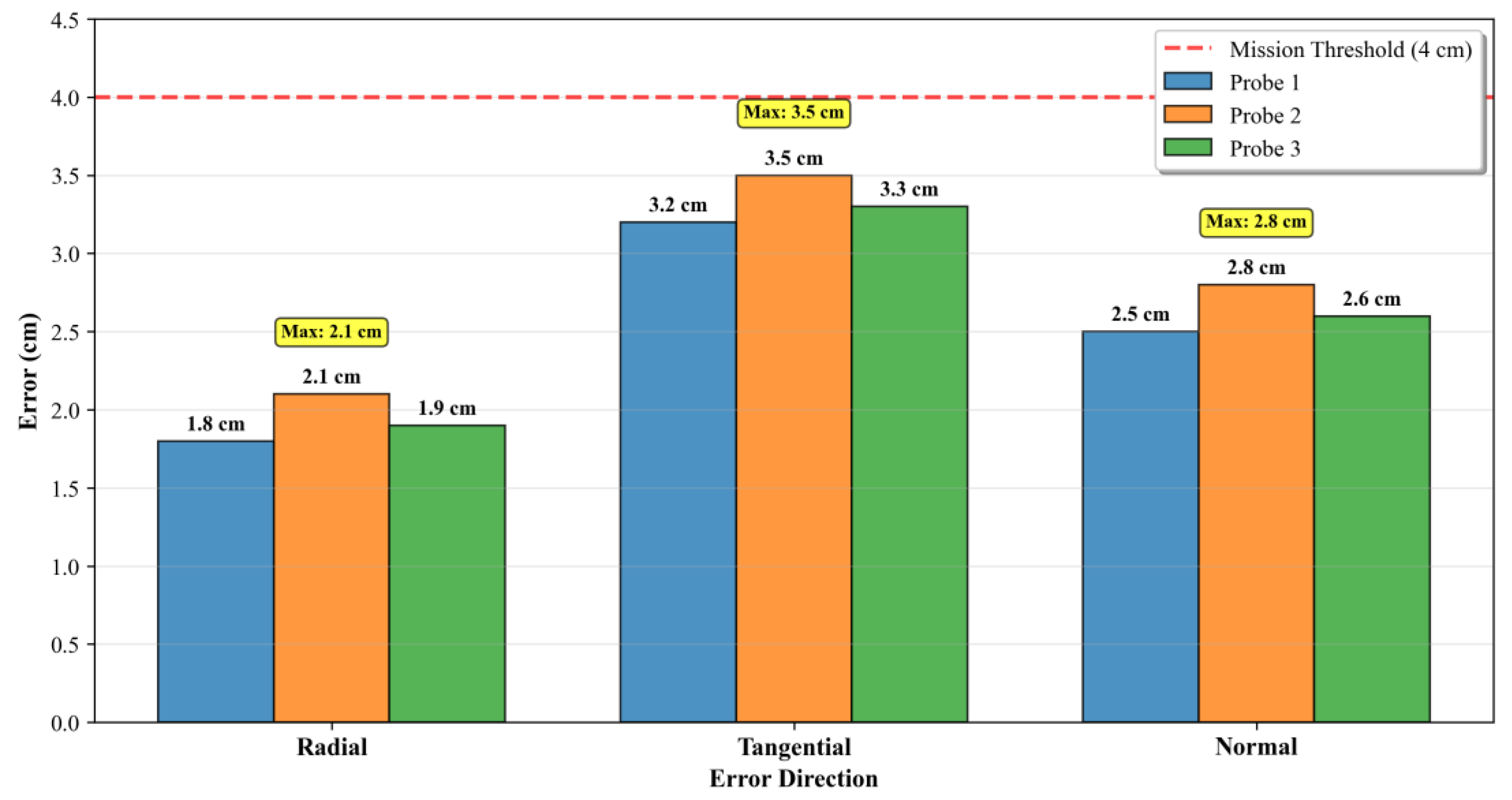
Furthermore, multi-node orbital consistency in the 1M3S configuration is evaluated using radial, tangential, and normal errors (Figure 8. Results indicate that the slave nodes exhibit radial errors < 2.1 cm, tangential errors < 3.5 cm, and normal errors < 2.8 cm relative to the master node—all well below the 15 cm threshold for collaborative operations. This confirms that calibrated model parameters effectively ensure orbital state consistency across multiple spacecraft, laying a foundation for subsequent collaborative missions.

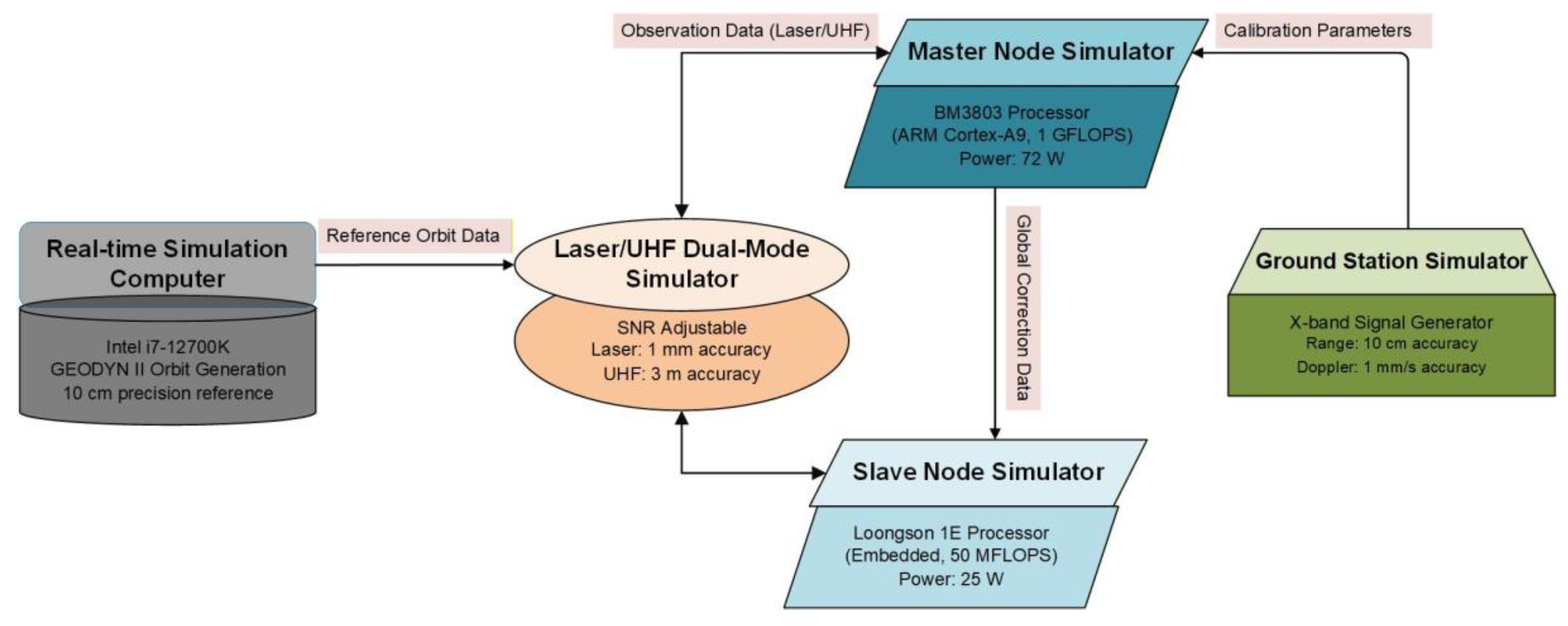
4.2. Hardware-in-the-Loop and Mission Data Replay Verification

To validate the proposed method’s engineering feasibility and real-world applicability under practical deep-space mission conditions, a hardware-in-the-loop (HIL) test platform was built (Figure 9). It comprises core components: master/slave node simulators, a laser/UHF dual-mode link simulator, a ground station emulator, and a real-time orbit generator (powered by GEODYN II software).

A 72-hour continuous operation test was conducted to assess long-term stability and real-time performance of the system. Specifically:

• 10 cm-level precision reference orbits were generated via GEODYN II, with input parameters including the GMM-2B gravity field, SRP model, and JPL DE436 ephemeris;
• During testing, observation data (with Gaussian white noise matching real measurement characteristics: 1 mm for laser ranging, 3 mm for UHF ranging, 10 cm for X-band ranging) and model errors (ΔJ₂₀ = 10⁻⁶, ΔCᵣ = 0.1, Δθ = 0.2°) were injected to simulate deep-space environmental conditions;
• The master node executed global orbit determination fusion every 4.8 minutes and dynamic model calibration every 10 minutes, while slave nodes performed local computation and compressed data transmission—no operational anomalies were recorded throughout the 72-hour duration.

Post-test analysis showed that the master node’s power consumption was constrained to 72 W (25 W per slave node), with absolute/relative orbit determination accuracies reaching 15.6 cm and 10.9 cm, respectively. Notably, this deviation of less than 8% from prior simulation results aligns with the low-power constraints of deep-space missions, directly confirming the method’s strong engineering implementability.

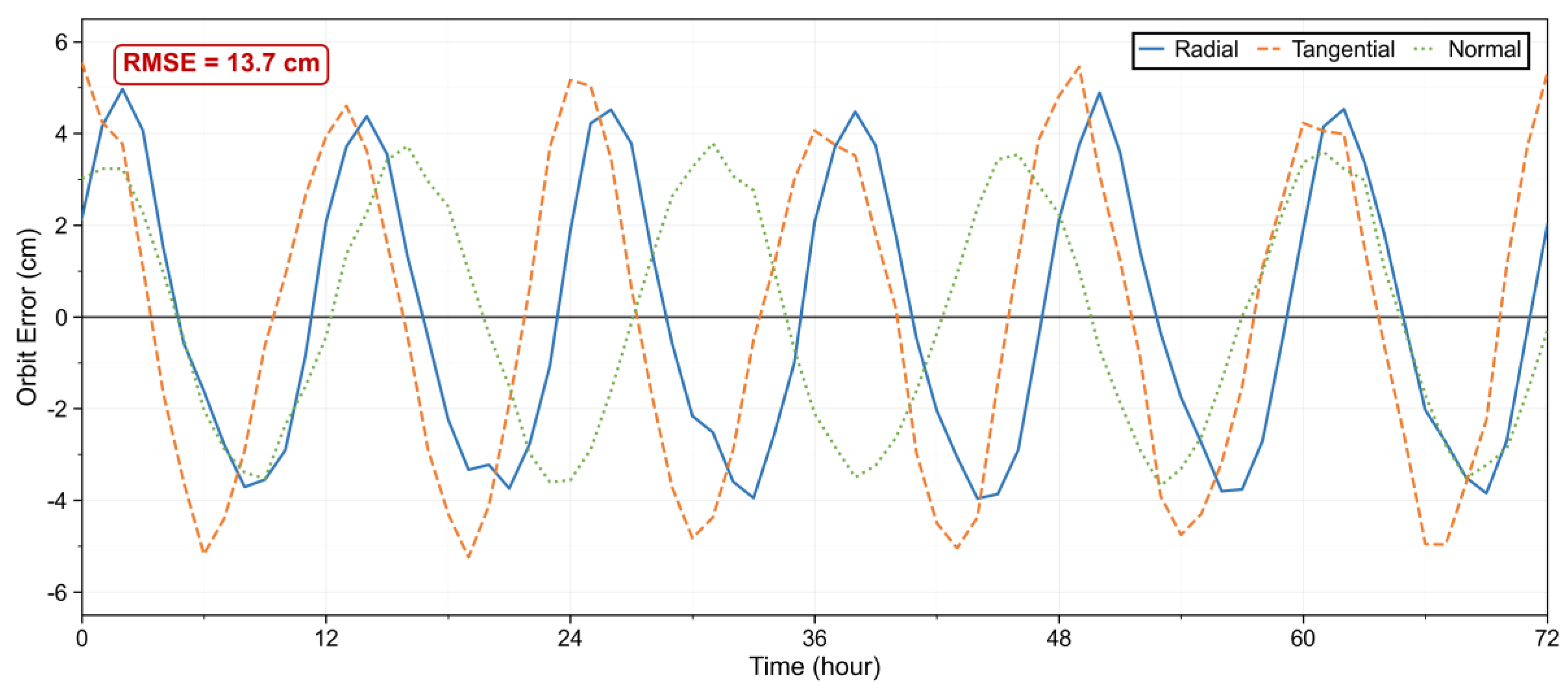
To further validate the proposed method under real mission conditions, we performed an orbit determination replay using actual telemetry data from the Tianwen-1 mission. The dataset, spanning seven consecutive days (sampling at 1 Hz) over three complete Mars orbital cycles during the relay communication phase [32,33]. This telemetry suite contained the same measurement types as used operationally: dual-frequency Doppler data (range accuracy ≈ 0.5 m), 1-second integrated two-way Doppler data (velocity accuracy ≈ 0.2 mm/s), and Very Long Baseline Interferometry (VLBI) delay data (time delay accuracy ≈ 0.3 ns). In the replay experiment, our framework employed identical force models—the GMM-2B Martian gravity field and the JPL DE436 planetary ephemeris—and the same attitude constraints as those used in the operational mission processing to ensure a consistent comparison. The replayed orbit solution achieved an absolute accuracy of 15.8 cm and a relative accuracy of 11.2 cm. This represents a 98.4% improvement over the official single-satellite orbit determination result (absolute accuracy >100 m) for the same Tianwen-1 mission phase. The RMSE between our replayed orbit and the official orbit was 13.7 cm. The radial, tangential, and normal components of the error all fluctuated around zero with no observable drift, confirming the scheme’s consistency and reliability when applied to real mission data (Figure 10).

These findings from both HIL testing and mission data replay collectively validate the proposed method’s reliability and effectiveness in practical deep-space mission contexts.

4.3. Comprehensive Comparison and Academic Positioning

This section positions the proposed framework within the current state of the art through a dual-level analysis: first, against ambitious deep-space mission profiles, and second, in methodological dialogue with cutting-edge distributed estimation research (2022–2025). We examine how existing approaches, while advanced in specific domains, often fail under the concurrent constraints of dynamic long-haul delays, weak-signal data intermittency, and stringent onboard resources—thereby justifying our integrated design.

4.3.1. Scenario Setup and Performance Comparison

Table 8 compares the proposed framework with representative international navigation schemes. Benchmarks such as NASA’s MSR achieve high precision (~15 cm absolute) but rely on ground-in-the-loop batch processing, limiting real-time multi-agent autonomy. Similarly, missions like ESA’s Hera employ CubeSat-grade hardware not designed for Mars-distance autonomy.

Table 8. Comparison of core performance metrics for deep-space multi-spacecraft orbit determination.

Scheme/Algorithm	Configuration	Absolute/Relative Accuracy (cm)	Key Assumptions/Limitations
Proposed Framework	1M3S (autonomous)	14.2±1.3/9.8±0.9	Idealized clock sync and observation geometry; validated via simulation with 35% ground coverage.
NASA’s MSR [1]	1M1S (ground-assisted)	~15/~10	Ground batch processing; limited autonomy. Normalized to 1M3S: ~9.3/~6.2 cm (redundancy model).
ESA Hera [4]	1M2S (CubeSats)	>100 (estimated)	CubeSat-grade sensors; not optimized for Mars-distance autonomy or dynamic delays.
ADMM-Based OD [30]	1M Multiple S	18.3/14.5	High computational load (~5 MFLOPS/node); partial delay adaptation (10–15 min range).
Deep Learning-Driven Nav [31]	Single/Dual	16.7/12.3	Data-intensive training; poor generalization in unexplored environments; no multi-node fusion.

Table 8. Comparison of core performance metrics for deep-space multi-spacecraft orbit determination.

Scheme/Algorithm	Configuration	Absolute/Relative Accuracy (cm)	Key Assumptions/Limitations
Proposed Framework	1M3S (autonomous)	14.2±1.3/9.8±0.9	Idealized clock sync and observation geometry; validated via simulation with 35% ground coverage.
NASA’s MSR [1]	1M1S (ground-assisted)	~15/~10	Ground batch processing; limited autonomy. Normalized to 1M3S: ~9.3/~6.2 cm (redundancy model).
ESA Hera [4]	1M2S (CubeSats)	>100 (estimated)	CubeSat-grade sensors; not optimized for Mars-distance autonomy or dynamic delays.
ADMM-Based OD [30]	1M Multiple S	18.3/14.5	High computational load (~5 MFLOPS/node); partial delay adaptation (10–15 min range).
Deep Learning-Driven Nav [31]	Single/Dual	16.7/12.3	Data-intensive training; poor generalization in unexplored environments; no multi-node fusion.

In contrast, the proposed framework delivers comparable centimeter-level precision within a fully autonomous, real-time multi-agent architecture. Co-designed and validated under low-power space-processor constraints (Section 4.2), this shift from ground-dominated to onboard autonomous estimation is essential for scalable missions such as asteroid swarm reconnaissance, where ground-control latency is prohibitive.

4.3.2. Methodological Positioning Against Cutting-Edge Academic Advances

• Delay Handling: Adaptive Weighting vs. Compensatory Consensus.

Recent approaches manage network delays through compensation or explicit modeling. Delay-aware consensus [34] and hybrid consensus filters [36] employ fixed compensation for bounded stochastic delays, while Gaussian feedback channel models [35] incorporate delay and bandwidth constraints in continuous time. However, under the extreme, deterministic, and variable delays (4–22 min) of Earth–Mars links, these mechanisms falter. In our identical 1M3S simulation (400 km orbit, 35% ground visibility, $\mathsf{\Delta }{J}_{20}={10}^{-6}$), applying the fixed compensation from [34] led to a performance degradation exceeding 58% across the delay range.

The TDA-FKF shifts from compensation to principled adaptation. It quantifies information timeliness via an Age-of-Information (AoI) inspired model, dynamically weighting stale ground data against fresh inter-satellite observations. This limits the accuracy degradation to only 33% (Table 5), offering a more stable solution when delay is a dominant system parameter.

2.

Robustness: Systemic Redundancy vs. Algorithmic Resilience.

Advanced robust filters, such as those using elliptical distributions [37] or resilient particle filters [38], tolerate outliers and data loss through statistical models. Their effectiveness, however, depends on data availability. In the same 1M3S scenario under a 10-minute laser outage, an architecture using only the algorithmic robustness of [37] degraded to 28.5 cm accuracy.

Our framework adopts a proactive, systemic approach. The heterogeneous dual-link (laser/UHF) provides physical-layer redundancy, while ARIMA-based hierarchical completion maintains >85% data availability before estimation. As shown in Figure 6, this strategy sustains 20.3 cm accuracy through the outage.

3.

Resource Efficiency: Cross-Layer Co-Design vs. Isolated Optimization.

Recent work reduces resource use through isolated techniques: event-triggered communication [39], clustering with compressive sensing [40], or lightweight filtering [41]. These do not holistically address the coupled data–computation–communication bottleneck in deep-space “one-master-multiple-slave” formations.

Our resource-aware architecture employs cross-layer co-design, concurrently reducing data volume by 74.7%, master-node computation to ~1.7 kFLOPS, and communication collisions from 18% to 2%. This synergy achieves high data freshness, low bandwidth use, and low computational latency with <5% precision loss, enabling stable 4.8-minute cycles (Figure 4), with the full methodological contrast detailed in Table 9.

Table 9. Methodological comparison with state-of-the-art academic algorithms.

Comparison Aspect	This Work (Deep-Space Tailored)	Representative Academic Approach [Ref.] & Core Trait	Key Differentiator & Quantitative Insight
Delay Philosophy	Timeliness-Quantified Adaptive Weighting	• AoI-based utility model • Dynamic space–ground weight optimization	Delay-Consensus Estimation [34]—Fixed compensation for bounded stochastic delays. Paradigm: Adaptation vs. compensation. Accuracy Degradation (4→22 min): 33% (Ours) vs. >58% (same simulation).
Robustness to Interruption	System-Level Redundancy & Proactive Completion	• Heterogeneous dual-link (Laser/UHF) • Predictive data completion (ARIMA)	Variational Bayesian Robust KF [37]—Algorithmic outlier tolerance. Layer: Physical/Data vs. Algorithm. Post 10-min Outage Accuracy: 20.3 cm (Ours) vs. 28.5 cm (same simulation).
Resource Efficiency	Cross-Layer Co-Design for Coupled Constraints	• Data: Covariance approx. + compression • Computation: Task redistribution + lightweight fusion • Communication: TDMA + priority scheduling	Event-Triggered Fuzzy Control [39]—Isolated communication saving. Scope: Holistic vs. isolated optimization. Master Node Compute: ~1.7 kFLOPS (Ours) vs. MFLOPS-range typical [46].

Table 9. Methodological comparison with state-of-the-art academic algorithms.

Comparison Aspect	This Work (Deep-Space Tailored)	Representative Academic Approach [Ref.] & Core Trait	Key Differentiator & Quantitative Insight
Delay Philosophy	Timeliness-Quantified Adaptive Weighting	• AoI-based utility model • Dynamic space–ground weight optimization	Delay-Consensus Estimation [34]—Fixed compensation for bounded stochastic delays. Paradigm: Adaptation vs. compensation. Accuracy Degradation (4→22 min): 33% (Ours) vs. >58% (same simulation).
Robustness to Interruption	System-Level Redundancy & Proactive Completion	• Heterogeneous dual-link (Laser/UHF) • Predictive data completion (ARIMA)	Variational Bayesian Robust KF [37]—Algorithmic outlier tolerance. Layer: Physical/Data vs. Algorithm. Post 10-min Outage Accuracy: 20.3 cm (Ours) vs. 28.5 cm (same simulation).
Resource Efficiency	Cross-Layer Co-Design for Coupled Constraints	• Data: Covariance approx. + compression • Computation: Task redistribution + lightweight fusion • Communication: TDMA + priority scheduling	Event-Triggered Fuzzy Control [39]—Isolated communication saving. Scope: Holistic vs. isolated optimization. Master Node Compute: ~1.7 kFLOPS (Ours) vs. MFLOPS-range typical [46].

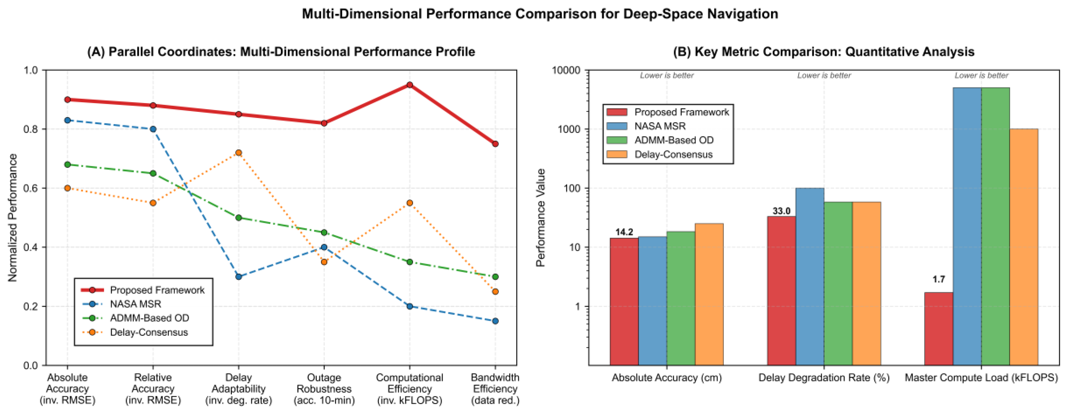
The Figure 11 visualizes performance across six normalized dimensions and three critical raw metrics. Data for this comparison are drawn from: experimental results for the Proposed Framework (Section 4.1), a normalized model for NASA’s MSR, and performance data for ADMM-Based OD [30] and Delay-Consensus [34], the latter two evaluated under identical simulation conditions to ensure a fair comparison. All schemes are assessed within the same 1M3S scenario, featuring a 400 km master orbit, 35% ground tracking coverage, and an initial dynamic model error of ΔJ₂₀ = 10⁻⁶.

4.3.3. Scenario Setup and Performance Comparison

The contribution is a triad-coherent design integrating three core innovations: a delay-aware fusion paradigm that transforms latency into an adaptive weighting parameter; a model-data dual-driven framework that ensures robustness through systemic redundancy and online calibration; and a resource-aware hierarchical architecture that resolves coupled constraints via cross-layer synergy.

This integrated blueprint bridges the gap between ground-reliant, high-precision orbit determination and fully autonomous, resource-limited onboard navigation. Rigorous simulation and validation (Section 4.1 and Section 4.2) demonstrate that centimeter-level, real-time, collaborative orbit determination is achievable within current deep-space spacecraft limits. The framework thus provides a validated technical foundation for future missions requiring high-precision multi-agent autonomy, such as Mars sample return, distributed asteroid reconnaissance, and cislunar constellations.

5. Discussion

The proposed scheme demonstrates significant advantages in multi-node autonomy, operational robustness, and engineering practicality, positioning it as a viable solution for next-generation deep-space orbit determination. These strengths stem from the integrated co-design of the TDA-FKF, dual-link fusion, dynamic model self-calibration, and hierarchical architecture, as validated by simulations, hardware-in-the-loop (HIL) tests, and mission replay. Its main strengths are fourfold:

• Strong adaptability to the “1M3S “ configuration, incorporating information compression (74.7% data volume reduction) and asynchronous fusion to shorten the solution cycle from 12.5 min (traditional FKF) to 4.8 min, improving overall processing efficiency by ~40%;
• High robustness under deep-space weak-signal conditions, maintaining stable accuracy (20.3 cm during 10-minute outages) with an 89% effective data rate—far higher than the 40–65% of single-link or ground-centric schemes;
• High engineering practicality, compatible with low-power space-qualified processors (≥50 MFLOPS, ≤10 W) such as ARM Cortex-A9 and Loongson-1E, validated via 72-hour HIL tests (15.6 cm/10.9 cm absolute/relative accuracy) and Tianwen-1 mission-data replay (15.8 cm/11.2 cm accuracy);
• A paradigm shift: moving from ground-dominated, post-facto batch processing (solution cycle >30 min) to onboard autonomous real-time determination with online self-calibration, eliminating reliance on real-time ground links (4–22 min delays) for centimeter-level accuracy.

Nevertheless, the current framework is optimized for a fixed 1M3S network topology, lacking adaptability to dynamic reconfiguration scenarios such as node failure, temporary detachment, or task-driven node addition/removal. To address this limitation and expand the framework’s applicability, future work will focus on two key directions: first, extending it to support dynamic topology via distributed consensus algorithms, aiming to achieve rapid state consistency convergence (<5 min) during reconfiguration without accuracy degradation (>15 cm); second, exploring Transformer-based temporal dependency modeling to enhance robustness during prolonged communication outages (>15 min), leveraging its ability to capture long-term orbital dynamics patterns for more accurate extrapolation (target accuracy <30 cm). These improvements will adapt the framework to more distant mission scenarios (e.g., Jupiter, asteroid exploration) with longer communication delays (>50 min) and sparser ground tracking (<20% visibility).

6. Conclusions

This work redefines the capabilities for real-time, collaborative orbit determination in deep space by integrating theoretical innovation, methodological synergy, and practical system design. The proposed hybrid framework demonstrates that centimeter-level accuracy is achievable autonomously onboard a resource-constrained multi-spacecraft formation, marking a shift from ground-dependent processing to an embedded, self-correcting navigation paradigm.

The contributions of this work are threefold and interrelated. Theoretically, it introduces a delay-aware fusion paradigm that quantifies the timeliness of information under variable interplanetary delays (4–22 min), providing a principled alternative to static weighting strategies. Methodologically, it establishes a model-data co-design framework, where orbital perturbation theory guides the online inversion of dynamic errors, and a resilient dual-link network ensures the necessary data integrity—jointly reducing model uncertainty by approximately 60%. Practically, it realizes a resource-aware distributed architecture that balances precision with efficiency through cross-layer optimizations, enabling the solution within strict onboard limits (e.g., ~1.7 kFLOPS for the master node) and improving multi-node fusion efficiency by 40%.

Validated through simulation, hardware-in-the-loop testing, and Tianwen-1 mission-data replay, the system achieves absolute and relative orbit accuracies of 14.2 cm and 9.8 cm in a 1M3S configuration—a performance gain exceeding 50% over traditional federated filters—while maintaining robust operation (20.3 cm accuracy) during 10-minute communication outages. These advances provide a critical, ready foundation for upcoming missions requiring high-precision multi-agent coordination, such as Mars sample return, distributed asteroid reconnaissance, and future cislunar navigation constellations.

References

- Sarli, B.; Bowman, E.; Cataldo, G.; Feehan, B.; Green, T.; Gough, K.; Hagedorn, A.; Hudgins, P.; Lin, J.; Neuman, M.; et al. NASA’s Capture, Containment, and Return System: Bringing Mars samples to Earth. Acta Astronaut. 2024, 223, 270–303. [Google Scholar] [CrossRef]
- Santoro, R.; Pontani, M. Orbit acquisition, rendezvous, and docking with a noncooperative capsule in a Mars sample return mission. Acta Astronaut. 2023, 211, 950–962. [Google Scholar] [CrossRef]
- Michel, P.; Küppers, M.; Bagatin, A.C.; Carry, B.; Charnoz, S.; de Leon, J.; Fitzsimmons, A.; Gordo, P.; Green, S.F.; Hérique, A.; et al. The ESA Hera Mission: Detailed Characterization of the DART Impact Outcome and of the Binary Asteroid (65803) Didymos. Planet. Sci. J. 2022, 3, 21. [Google Scholar] [CrossRef]
- Lodiot, S.; Guerbuez, C. Hera ESOC/ESA Operations: First Months in Flight and Asteroid Phase Planning Concepts. Space Sci. Rev. 2025, 221, 7. [Google Scholar] [CrossRef]
- Takeuchi, H.; Yoshikawa, K.; Takei, Y.; Oki, Y.; Kikuchi, S.; Ikeda, H.; Soldini, S.; Ogawa, N.; Mimasu, Y.; Ono, G.; et al. The deep-space multi-object orbit determination system and its application to Hayabusa2’s asteroid proximity operations. Astrodynamics 2020, 4, 377–392. [Google Scholar]
- Duffy, L.; Adams, J.; Sega, R.M. Optimized Design of an Integrated Cislunar Communication, Navigation, and Domain Awareness System of Systems. Int. J. Aerosp. Eng. 2025, 2025, 12. [Google Scholar] [CrossRef]
- Lv, H.J.; Xing, N.; Huang, Y.; Li, P.J. Precise Orbit Determination for Cislunar Space Satellites: Planetary Ephemeris Simplification Effects. Aerospace 2025, 12, 716. [Google Scholar] [CrossRef]
- Gill, E.; Montenbruck, O.; Arichandran, K.; Tan, S.H.; Bretschneider, T. High-Precision Onboard Orbit Determination for Small Satellites—The GPS-Based XNS on X-SAT. In Proceedings of the Symposium on Small Satellites Systems & Services, La Rochelle, France, 20–24 September 2004; 2004; Volume ESA-SP 571, p. 47. [Google Scholar]
- WU, W.; LI, H.; LI, Z.; WANG, G.; TANG, Y. Status and prospect of China’s deep space TT&C network. SCIENTIA SINICA Informationis 2020, 50, 87–127. [Google Scholar] [CrossRef]
- Konopliv, A.S.; Asmar, S.W.; Folkner, W.M.; Karatekin, Ö.; Nunes, D.C.; Smrekar, S.E.; Yoder, C.F.; Zuber, M.T. Mars high resolution gravity fields from MRO, Mars seasonal gravity, and other dynamical parameters. Icarus 2011, 211, 401–428. [Google Scholar] [CrossRef]
- Cao, J.; Li, X.; Ju, B.; Man, H.; Zhang, Y.; Liu, S. Multi-satellite Precision Orbit Determination and Data Analysis Software in Solar System. J. Deep. Space Explor. 2022, 9, 532–541. [Google Scholar] [CrossRef]
- Carlson, N.A. Federated square root filter for decentralized parallel processors. IEEE Trans. Aerosp. Electron. Syst. 1990, 26, 517–525. [Google Scholar] [CrossRef]
- Carlson, N.A.; Berarducci, M.P. Federated Kalman Filter Simulation Results. J. Inst. Navig. 1994, 41, 297–312. [Google Scholar] [CrossRef]
- Liggins, M.E.; Chee-Yee, C.; Kadar, I.; Alford, M.G.; Vannicola, V.; Thomopoulos, S. Distributed fusion architectures and algorithms for target tracking. Proc. IEEE 1997, 85, 95–107. [Google Scholar] [CrossRef]
- Gao, Z.; Mu, D.; Zhong, Y.; Gu, C.; Ren, C. Adaptively Random Weighted Cubature Kalman Filter for Nonlinear Systems. Math. Probl. Eng. 2019, 2019, 4160847. [Google Scholar] [CrossRef]
- Zhang, Z.; Li, Q.; Han, L.; Dong, X.; Liang, Y.; Ren, Z. Consensus Based Strong Tracking Adaptive Cubature Kalman Filtering for Nonlinear System Distributed Estimation. IEEE Access 2019, 7, 98820–98831. [Google Scholar] [CrossRef]
- Fraser, C.T.; Ulrich, S. Adaptive extended Kalman filtering strategies for spacecraft formation relative navigation. Acta Astronaut. 2021, 178, 700–721. [Google Scholar] [CrossRef]
- Li, X.; Zhang, K.; Ma, F.; Zhang, W.; Zhang, Q.; Qin, Y.; Zhang, H.; Meng, Y.; Bian, L. Integrated precise orbit determination of multi-GNSS and large LEO constellations. Remote Sens. 2019, 11, 2514. [Google Scholar] [CrossRef]
- Kang, Z.G.; Tapley, B.; Bettadpur, S.; Ries, J.; Nagel, P.; Pastor, R. Precise orbit determination for the GRACE mission using only GPS data. J. Geod. 2006, 80, 322–331. [Google Scholar] [CrossRef]
- Arnold, D.; Montenbruck, O.; Hackel, S.; Sosnica, K. Satellite laser ranging to low Earth orbiters: Orbit and network validation. J. Geod. 2019, 93, 2315–2334. [Google Scholar] [CrossRef]
- Lombardo, M.; Zannoni, M.; Gai, I.; Gomez Casajus, L.; Gramigna, E.; Manghi, R.L.; Tortora, P.; Di Tana, V.; Cotugno, B.; Simonetti, S.; et al. Design and Analysis of the Cis-Lunar Navigation for the ArgoMoon CubeSat Mission. Aerospace 2022, 9, 659. [Google Scholar] [CrossRef]
- Hinga, M.B.; Williams, D.A. Autonomous Lunar L1 Halo Orbit Navigation Using Optical Measurements to a Lunar Landmark. Navigation 2023, 70, 30. [Google Scholar] [CrossRef]
- Ely, T.A.; Seubert, J.; Bradley, N.; Drain, T.; Bhaskaran, S. Radiometric Autonomous Navigation Fused with Optical for Deep Space Exploration. J. Astronaut. Sci. 2021, 68, 300–325. [Google Scholar] [CrossRef]
- Nesnas, I.A.D.; Hockman, B.J.; Bandopadhyay, S.; Morrell, B.J.; Lubey, D.P.; Villa, J.; Bayard, D.S.; Osmundson, A.; Jarvis, B.; Bersani, M.; et al. Autonomous Exploration of Small Bodies Toward Greater Autonomy for Deep Space Missions. Front. Robot. AI 2021, 8, 26. [Google Scholar] [CrossRef]
- Andolfo, S.; Genova, A.; Federici, P.; Teodori, R.; Cottini, V. Precise orbit determination through a joint analysis of optical and radiometric data. In Proceedings of the International Conference on Space Robotics (iSpaRo), Luxembourg, 24–27 June 2024; pp. 28–35. [Google Scholar] [CrossRef]
- Hanson, B.L.; Ely, T.A.; Bewley, T.R.; Rosengren, A.J. Bayesian Benchmarking of GBEES Applied to Outer Planet Orbiter Estimation. J. Guid. Control Dyn. 2025, 7. [Google Scholar] [CrossRef]
- Wu, C.Y.; Han, S.; Chen, Q.; Wang, Y.; Meng, W.X.; Benslimane, A. Enhancing LEO Mega-Constellations with Inter-Satellite Links: Vision and Challenges. IEEE Wirel. Commun. 2025, 32, 196–202. [Google Scholar] [CrossRef]
- Konopliv, A.S.; Park, R.S.; Folkner, W.M. An improved JPL Mars gravity field and orientation from Mars orbiter and lander tracking data. Icarus 2016, 274, 253–260. [Google Scholar] [CrossRef]
- Pavlis, D.E.; Merrick, A.A.; McCarthy, J.J.; et al. GEODYN II System Description; NASA/GSFC: Greenbelt, MD, USA, 2013. [Google Scholar]
- Boyd, S.; Parikh, N.; Chu, E.; Peleato, B.; Eckstein, J. Distributed Optimization and Statistical Learning via the Alternating Direction Method of Multipliers. Found. Trends Mach. Learn. 2011, 3, 1–122. [Google Scholar] [CrossRef]
- Song, J.; Rondao, D.; Aouf, N. Deep learning-based spacecraft relative navigation methods: A survey. Acta Astronaut. 2022, 191, 22–40. [Google Scholar] [CrossRef]
- Huang, X.Y.; Xu, C.; Guo, M.W.; Li, M.D.; Hu, J.C.; Wang, X.L.; Zhao, Y.; Liu, W.W. Tianwen-1 Entry, Descent, and Landing Guidance, Navigation, and Control System Design and Validation. J. Spacecr. Rocket 2023, 60, 1983–2002. [Google Scholar] [CrossRef]
- Man, H.; Cao, J.; Ju, B.; Li, X.; Kong, J.; Liu, S. “Tianwen-1” Detector Orbit Determination and Accuracy Evaluation. Acta Geod. Cartogr. Sin. 2024, 53, 1288–1297. [Google Scholar] [CrossRef]
- Wang, Q.Y.; Meng, M. Distributed nonlinear estimation with communication delays. J. Control Decis. 2025, 12. [Google Scholar] [CrossRef]
- Liu, Z.Y.; Conti, A.; Mitter, S.K.; Win, M.Z. Continuous-Time Distributed Filtering via a Gaussian Feedback Channel. IEEE J. Sel. Areas Commun. 2025, 43, 3410–3425. [Google Scholar] [CrossRef]
- Huang, F.J.; Wu, P.L.; Li, X.X.; He, S.; Kong, L.Q. Hybrid consensus information filter under limited bandwidth for maneuvering target tracking. Proc. Inst. Mech. Eng. Part G–J. Aerosp. Eng. 2025, 239, 2511–2524. [Google Scholar] [CrossRef]
- Wang, A.J.; Jiang, Z.H.; Zhou, W.D.; Wang, D.S.; Jia, G.L. Centralized and Distributed Variational Bayesian Robust Kalman Filter Under Elliptical Distribution With Inaccurate Noise Covariance Matrices. IEEE Internet Things J. 2025, 12, 47151–47162. [Google Scholar] [CrossRef]
- Gao, X.B.; Gao, L.; Zhai, Y.F.; Li, G.C.; Wei, P. A resilient distributed particle filter over sensor networks. Inf. Fusion 2026, 127, 10. [Google Scholar] [CrossRef]
- Gong, H.B.; Hao, L.Y.; Li, Y.X. Dynamic event-triggered distributed fuzzy H∞ optimal formation control for input-constrained underactuated AUVs with unknown dynamics. Neurocomputing 2026, 661, 12. [Google Scholar] [CrossRef]
- Wang, H.T. Energy efficient data transmission scheme integrating clustering and compressive sensing in wireless sensor networks. Comput. J. 2025, 68, 1345–1354. [Google Scholar] [CrossRef]
- Liu, Y.; Wang, Z.D.; Hu, J.; Chen, Y.; Dong, H.L. Distributed maximum correntropy filtering for a class of multi-rate systems over sensor networks. Inf. Fusion 2026, 127, 11. [Google Scholar] [CrossRef]
Figure 1.
Overall architecture of the “one-master, multiple-slave” hybrid JOD system. The diagram depicts a four-node spacecraft constellation consisting of one primary orbiter and three secondary probes. Layers include the onboard autonomous processing layer, inter-satellite data exchange layer, ground-based delay calibration layer, and hierarchical fusion layer. The master node integrates global fusion and model calibration modules, while the slave nodes host local processing units. Laser master links (solid lines) and UHF backup links (dashed lines) form the inter-satellite network. The ground station supplies calibration parameters to the master node.
Figure 2.
Workflow of the TDA-FKF, illustrating the closed–loop “local computation–centralized fusion–feedback calibration” architecture.
Figure 3.
Adaptive weighting strategy of the TDA-FKF in response to Earth-Mars communication delay.
Figure 4.
Performance benchmarking of communication efficiency: A comparative analysis between the traditional FKF and the proposed scheme for the “1M3S” configuration.
Figure 5.
Evolution of the minimum eigenvalue λmin of the Fisher Information Matrix for different inter-satellite link configurations. The dual-link architecture (Scenario (A)) provides persistently stronger observability than any single-link configuration (B,C). The absence of inter-satellite links (D) leads to periods of very weak observability.
Figure 6.
Robustness evaluation under communication impairment. Comparison of absolute orbit determination accuracy (RMSE) during a simulated 10-minute laser link outage between the complete system (Proposed-Full) and the system without dual-link fusion capabilities (Ablated-Dual Link). The complete system maintains stable accuracy at approximately 20.3 cm by utilizing UHF backup links and ARIMA-based data completion. In contrast, the ablated system suffers severe performance degradation, with accuracy deteriorating to 38.6 cm (representing a 90% increase in error relative to its initial performance). This result quantitatively demonstrates the critical role of heterogeneous link fusion in ensuring navigation continuity under deep-space weak-signal condition.
Figure 7.
Orbit determination accuracy degradation curves under observation outage scenarios. Horizontal axis represents observation outage time (0–15 minutes), vertical axis represents absolute orbit determination accuracy (RMSE, cm). Our scheme curve appears gentle, traditional FKF curve steep, annotating 10-minute, 15-minute accuracy values, highlighting robustness advantages.
Figure 8.
Multi-node orbital consistency errors in the “1M3S” configuration. Bar chart displaying radial, tangential, and normal errors of three slave nodes relative to the master node. The inner circle represents the 4 cm mission consistency threshold, verifying that all errors meet collaborative operation requirements.
Figure 9.
Hardware composition of Hardware-in-the-Loop test platform. Illustrates the platform’s hardware layout, annotating connections and core parameters of master-slave node simulators, laser/UHF simulators, and tracking station simulators, and explaining the function of the real-time simulation computer.
Figure 10.
Replayed orbit versus Tianwen-1 orbit error comparison. Displays radial, tangential, and normal errors over time, annotating an RMSE of 13.7 cm, and showing that errors fluctuate around zero without significant drift.
Figure 11.
Parallel coordinates plot and key metric comparison. (A) Parallel coordinates plot of the four navigation schemes across six normalized performance dimensions. The proposed framework (red solid line) demonstrates a consistently balanced and superior profile across all constraints, whereas benchmark schemes exhibit significant trade-offs (e.g., high accuracy at the cost of resource efficiency for NASA’s MSR). (B) Bar chart comparing three critical metrics: absolute positioning accuracy (lower RMSE is better), delay-induced accuracy degradation rate (lower is better), and master node computational load (lower kFLOPS is better). Error bars denote standard deviations from Monte Carlo simulations.