Submitted:
20 November 2024
Posted:
21 November 2024
You are already at the latest version
Abstract
LEO satellites offer reduced signal loss, fast movement, multi-beam, typically providing single coverage. This paper introduces a novel multi-beam power positioning method for low-orbit single-satellite, addressing the slow convergence and low accuracy of Doppler positioning. It establishes a power observation equation system, initializes with the nearest neighbor algorithm, and refines with the least squares method. Monte Carlo simulations indicate that with good initial values, the method converges in under 10 iterations, achieving 88.06% availability at 20° elevation with errors of 5331m (vertical) and 8798m (horizontal), and a timing error of 205μs. At 70° elevation, all users converge with errors of 1614m and 1088m, and a timing error of 31.3μs, demonstrating high power positioning availability. The statistical results show that power positioning users can obtain the positioning accuracy of kilometers and the timing accuracy of microseconds, which meets initial timing needs under strong confrontation, enhancing the medium and high orbit satellite navigation.
Keywords:
LEO satellites
; multi-beam
; power positioning
1. Introduction
Low Earth Orbit (LEO) satellites, as an emerging navigation enhancement method, possess many unique advantages. Their orbital altitude is relatively low, and the signal power is high, with the ground power being about 30dB higher than that of GNSS, resulting in high signal quality and strong anti-interference capabilities, enabling services to be provided indoors and in obstructed areas [1]. The greatest advantage of LEO satellites is their fast movement speed, which can greatly reduce the correlation between adjacent observation epochs, achieving rapid convergence in positioning [2], and the large Doppler shift, which offers good Doppler observation [3].
Based on the characteristics of LEO satellites, with a sufficient number of satellites, LEO navigation constellations can perform independent positioning and timing, or combined positioning and timing with GNSS, using traditional positioning algorithms such as pseudorange positioning and carrier phase positioning to achieve navigation enhancement [4]. The analysis of the combined positioning effects of LEO satellites with different orbital heights and GNSS constellations shows that LEO satellites have low orbits and fast geometric motion speeds, with the geometric dilution of precision (GDOP) value changing rapidly, effectively shortening the convergence time for GPS/BDS positioning. The enhancement effect of different numbers of LEO satellites on GNSS is significantly different, with more satellites leading to more noticeable enhancement effects. Additionally, multi-satellite Doppler positioning technology has become a research hotspot in the application of LEO satellite constellations in recent years. Morales-Ferre et al. [5] compared the code-GDOP and Doppler-GDOP in the Amazon Kuiper and SpaceX StarLink constellations. The Doppler-GDOP values are significantly larger than the code-GDOP values, indicating that the accuracy of LEO satellite Doppler positioning is more sensitive to observation errors. McLemore and Psiaki [6] analyzed the GDOP of LEO constellations, using a new Doppler positioning model that simultaneously utilizes Doppler shift and pseudorange measurements to estimate position vector components, receiver clock bias, velocity vector components, and receiver clock bias rate. Tan et al. [7] analyzed the impact of measurement errors, satellite orbit errors, and constellation geometric distribution on LEO Doppler positioning. Guo [8] pointed out that the accuracy of multi-satellite Doppler positioning can be comparable to GNSS pseudorange positioning under conditions of low observation noise. Matteo Sgammini et al. explored the application of satellite Doppler positioning technology in vehicle navigation, proposing a high-precision vehicle navigation system based on satellite Doppler positioning [9].
However, for LEO satellite constellations, if the GNSS pseudorange-based time difference positioning method is still used, the system's requirement for time synchronization is very high, which will greatly increase the system construction cost [10]. When the number of visible satellites is insufficient, and users do not meet the conditions for multiple coverage, both pseudorange positioning and carrier phase positioning are not available. In this case, single-satellite Doppler positioning requires a relatively long observation time for the satellite, using integrated Doppler for positioning solution, which is not real-time [11], has a long convergence time, and low precision, and has certain application limitations.
To meet the rapid positioning needs of LEO users, it is possible to consider using the power measurements of multi-beam signals to calculate the user's approximate position. Since the transmission antenna of LEO satellites adopts a beam scanning broadcast method, during the satellite's movement, the received power of the receiver at different positions on the Earth's surface at different times has certain differences, and the magnitude of these differences is related to the beam width and beam pattern. Therefore, users can receive different received power measurements from different beams of a single LEO satellite to establish a fingerprint library.
Current research on power matching positioning is focused on indoor positioning, as multiple WiFi Access Points can be detected indoors, and their signals are easy to measure, making the fingerprint positioning method based on Received Signal Strength Indication one of the most popular positioning technologies today [12]. This method is typically divided into offline and online stages: the offline stage collects the received signal strength at reference points in the positioning area as a fingerprint library; the online stage obtains real-time positioning data and matches it with the fingerprint library to obtain the estimated location [13].
Traditional power matching positioning uses different indices to calculate the similarity between fingerprint vectors and observation vectors, such as Euclidean distance [14], cosine similarity, Pearson coefficient [15], and other methods, most of which use direct differential calculations. However, it is difficult to accurately describe the complex nonlinear relationships between signal vectors. Therefore, many scholars are currently using machine learning (ML) and deep learning (DL) for neighbor point matching. It can be roughly divided into two groups: one group is supervised learning methods, which use various classification methods such as random forests (RF), decision trees (DT), Bayesian, support vector machines, neural networks (NN), convolutional neural networks (CNN), and other classification algorithms [16,17]. The other is unsupervised learning methods that use clustering, K-Means [18], fuzzy clustering [19], and density-based noise application spatial clustering [20], among other methods. These classification and clustering schemes are expected to use a shorter time to judge the test set after the database is formed, thereby obtaining the user's approximate location.
For the first time in the context of LEO satellite scenarios, this paper proposes the use of multi-beam signal power measurements for positioning and timing. Based on traditional satellite navigation system algorithms, the nearest neighbor algorithm is used to solve for initial values, and the least squares method is used for iterative solution, including the linearization of nonlinear equation systems, solution of linear equation systems, updating the roots of nonlinear equation systems, and judging the convergence of iterations. It is possible to use power measurements for single-point rapid positioning of users under a single LEO satellite scenario, with the expectation that some users will achieve better positioning and timing performance.
2. Materials and Methods
2.1. Multi-Beam Signal Power Observation Model
The power measurement of the multi-beam satellite signal received by the user is related to the user's elevation angle , the satellite azimuth angle , the satellite elevation angle and the user's geodetic height , which can be expressed as:
Among them, the multi-beam number representing the signal transmitted by the satellite. represents the EIRP value of the satellite transmitted signal, represents the spatial transmission loss of the satellite signal related to the user's elevation angle and ground height, and represents the gain value of the user's receiving antenna.
The EIRP value of the satellite transmitted beam signal and the gain value of the user's received antenna , can usually be obtained by antenna simulation or actual measurement, and it is assumed that the accurate modeling of both has been completed, and the modeling error is ignored.
When the satellite position is known, the user's position can be determined by the satellite elevation angle , the satellite azimuth angle and the distance between the user and the satellite, and when the three-dimensional position of the satellite in the ECEF coordinate system is known, the three-dimensional position of the user in the ECEF coordinate system can be obtained by using the geometric relation. Figure 1 below shows the geometric relationship between the user and the satellite, where is the radius of the earth, is the orbital height of the satellite, is the geodetic height of the user, and is the distance between the user and the satellite. Firstly, the relationship between the elevation angle of the user and the expansion angle of the satellite beam is derived.
The geometric relationship shown in the figure above, according to the sinusoidal theorem, can be obtained:
Therefore, it is possible to derive the satellite beam tension angle as:
when the elevation angle of the user is valued between 0 and 90, it is not difficult to conclude that the elevation angle of the user corresponds to the value of the satellite elevation angle from the function relationship.
The space transmission loss of satellite signals is deduced below, and the distance from the satellite to the user is calculated first. According to the geometric relationship shown in Figure 1, and according to the cosine theorem, we can get:
Further, the distance from the user to the satellite can be calculated as:
According to Friis transmission equation, the power in the fixed solid angle remains the same. Therefore, the spatial transmission loss of signal power at a point on the spherical surface with a radial of the transmitting antenna is:
where refers to the wavelength.
2.2. Power Perception Measurement Error Model
After receiving the signal from the satellite, the user usually measures the power of the received signal by matching the reception. Assuming that the user has completed the time and frequency synchronization of the satellite signal, and stripped away the possible pseudo-random codes and Doppler frequencies that may be modulated on the signal, while ignoring the influence of the transmitted message symbol, the user's received signal can be expressed as:
where the amplitude of the received signal is denoted by the thermal noise error of the power is denoted by which generally obeys a normal distribution.
Considering that the thermal motion of charged particles in a circuit forms thermal noise, the noise power is usually expressed as the noise temperature corresponding to the thermal noise power of the same magnitude, and the relationship between them is as followed:
The unit of is Watts(W), the unit of is Kelvin (K) and the unit of noise bandwidth is Hertz(Hz).The Boltzmann constant is equal to J/K, which is taken as 290K at room temperature.
When the duration of the signal power measurement is , it is advisable to assume that the user takes the coherent integration method to estimate the signal amplitude, then there are:
where is the measured value of the amplitude of the received signal. is the coherent integrated noise, and its equivalent noise bandwidth is taken . Before and after coherent integration, the signal power, amplitude, and noise power spectral density do not change, but because the noise bandwidth before the correlator is , and the filtering bandwidth of the coherent integrator can be regarded as , the narrowing of the noise bandwidth must cause a decrease in the noise power, so the noise power after coherent integration is reduced to .
2.3. A System of Equations for Power Observations
When the user receives multiple beamed satellite signals and measures the signal power, the equation is as follows:
Among them, is the power measurement of different beams, and the power observation noise of different beams.
the power observation equation for the other beams is different from the observation equation for beam 1, the difference between other beams and beam 1 is calculated by:
where, take ,.
Assuming that the initial values of and are and , where the system of equations is linearized and expanded, then there is:
where , and cause:
Then the above equation can be rewritten as:
Further, it can be solved that:
2.4. Power Positioning Algorithm Solution Process
Since multi-beam power positioning is applied to low-orbit satellite scenarios, the quality of the received signal is poor when the user's elevation angle is too low, thus the simulation parameters are set as Table 1:
The input required for the power positioning least squares algorithm is the initial value of the satellite elevation angle , the initial value of the azimuth angle , the ERIP value of k beams of prior information , and the user gain .Figure 2 gives the flowchart of the algorithm:
The least-squares algorithm itself outputs the satellite tension angle and azimuth angle, however, we need to obtain the user's vertical and horizontal information. It is worth noticing that in the process of calculating the elevation angle of the user, h=0 is first assumed, which is due to the negligible altitude of the user's geodetic altitude in relation to the radius of the Earth and the orbital height of the satellite. The h after the least squares solution is obtained by a series of calculations such as link loss, and the two values are not contradictory, and the analysis of the error in the following is based on the h of the least squares solution.
Substituting equation (2), we can get the elevation angle from the user to the satellite as:
According to equation (4), the user's geodetic height can be calculated as:
The user vertical information is:
In order to facilitate the subsequent analysis of the power positioning timing performance, the evaluation index of the positioning result error is defined here, assuming that the true value of the satellite elevation angle is and the solution value is , then the elevation angle error is .
If there are users in different locations, the statistical positioning performance of these users can be given by the error deviation and the standard deviation, which is defined as follows:
Satellite azimuth error, user horizontal error, user vertical error and their deviation are defined as above.
3. Results
3.1. Least Squares Initial Value Requirements and Acquisition
In the process of power positioning solution, the initial conditions have a great influence on the results, and the better initial conditions can make the iteration converge quickly, and the poor initial conditions will greatly reduce the iteration speed, and even the convergence results cannot be obtained in the end. Due to the characteristics of planar phased array antennas, ground users may have the same receiving power in different areas, and if the gap between the initial position and the user's position is too large, the solution is easy to fall into the local optimal solution, resulting in a large positioning error.
3.1.1. Least Squares Solves the Initial Value Requirements
Assuming that the user elevation angle is 40(converted to the satellite elevation angle is 40.04) and the satellite azimuth angle is 30, after 10 least squares iterations, Figure 3 shows the convergence and divergence over the course of 10 least squares iterations:
It can be observed that when the initial values are set close to the true values, the iteration tends to converge; when the initial values are set far from the true values, the least squares iteration diverges. Consequently, the power positioning least squares scheme has certain requirements for initial values.
To determine these requirements, it is assumed that the true elevation and azimuth angles of the satellite are , the initial value is set to a certain value below the true value, and the positioning results of multiple Monte Carlo simulations are required to converge to within the range of the true value of 1, that is , the initial value requirements of the least squares method at this time are required a and b, where a is the initial value requirement of the satellite elevation angle, and b is the initial value requirement of the satellite azimuth angle.
In the simulation, users with poor observation quality due to low elevation angles are excluded. By iterating over user elevation angles α in the range [10°, 90°] (which corresponds to satellite elevation angles γ in the range [0°, 55.8°]), and satellite azimuth angles β in the range [1°, 360°], we can statistically determine the initial value requirements a and b for the power matching least squares method.
The statistical results of the initial value of least squares solution requirements are shown in the Figure 4:
It is not difficult to see that when the initial values of elevation angle and azimuth angle are below the true value of 2°, it can be considered that the vast majority of users (94.5% and 93.2%) can use power matching positioning to perform least squares solution and obtain a convergence solution. The solution to meet the initial value requirements can be obtained by using user prior information or other algorithms.
3.1.2. Initial Values of the Iteration by the Nearest Neighbor Algorithm Obtains
This section introduces the method of obtaining the initial value that satisfies the convergence condition of least squares solution, and briefly explains the nearest neighbor algorithm (K value takes 1 in KNN) as an example, and then considers different fingerprint database frameworks and parameters.
According to the system of power measurement equations (10), based on the EIRP information of each beam known on the satellite side, the theoretical received power values of users at different locations can be solved through the link budget, and in fact, for a single user, the received power of up to M beams can be obtained. When the user's fingerprint location information is the real user location, there will only be one noise deviation between the theoretical received power value of M and the actual received power value of a single user, which is very small and negligible in most cases, which is called positioning matching. However, when the user location fingerprint is different from the real user location, there will always be a large difference between the theoretical received power value and the actual received power value of some beams of a single user, which is called mismatch.
Considering the processing time of the nearest neighbor algorithm and the actual user situation, the power fingerprint database in this paper traverses the elevation angles of different users and takes a certain azimuth interval to establish it. In the matching process, the azimuth interval can be initialized by a priori known information, and then the azimuth search interval can be gradually narrowed to achieve more accurate and robust matching results.
In the simulation, we traverse the user's elevation angle (converted to a satellite elevation angle of [0,55.8]), the satellite azimuth angle , and the user's ground height are all set to 0m. Assuming that the user's elevation angle is unknown and the azimuth uncertainty is 5, there are 72 different fingerprint databases, each of which contains all the user's elevation angle information and a certain azimuth information. In order to reduce the influence of noise on the nearest neighbor algorithm, the width of the fingerprint library is taken as 10 beams, which are the 10 largest beam points among the M received power obtained by each user.
The simulation results of the nearest neighbor algorithm power matching localization are as Figure 5 and Figure 6:
The colorbar depth of the above two graphs represents the azimuth and vertical error of the satellite, and the darker the color, the smaller the error. It can be seen that the error of satellite elevation angle is small, generally below 0.5, while the azimuth error of satellite is large, generally above 0.5, and the error under the condition of high user elevation angle is significantly increased, which is mainly due to the fact that the beam receiving power of users with high elevation angle is generally large, and it is difficult to distinguish the difference of beam between different users, resulting in some misjudgments in the algorithm. In general, the power matching positioning of the nearest neighbor algorithm can meet the requirements of the least-squares algorithm for the initial value of convergence.
3.2. Analysis of Single-User Positioning Error
Assumed the satellite angle errors are , the power calculation error is ,if error terms are taken into account:
From the previous Newtonian iterative process, it can be deduced that the relationship between the elevation angle and azimuth angle of the two satellites directly related to the user's position and the power calculation error is as follows:
Assuming that the parameters remain unchanged during the receiver receiving the satellite signal, and each observation value is independent of each other, the observation error obeys the standard normal distribution, the mean value is 0, and the variance is . So the covariance of can be expressed as:
Taking the user's elevation angle of 60 (converted to a satellite elevation angle of 24.882), the satellite azimuth angle of 30, and the geodetic height of 0m as an example, the receiver sensitivity is set to -160dBm, and the results of multiple Monte Carlo simulations are as follows:
As can be seen from the figure above, the satellite tension angle and azimuth results of multiple Monte Carlo simulations are around the true value, and their statistical mean values can converge to within the range of 0.5 of the true value. The vertical and horizontal error of a single Monte Carlo simulation is not more than 40km, and its statistical average value can converge to within the range of 50km of the true value, and the power positioning algorithm tends to converge, so the user can use the power positioning timing method to perform multiple positioning solutions to achieve better positioning performance. The results of 1000 Monte Carlo simulations are statistically analyzed, and the probability distribution functions of each parameter are fitted as follows:
The normal fitting of satellite azimuth angle , user vertical difference , and horizontal difference is good. The solved satellite azimuth angle is approximately normally distributed as , and the elevation angle is approximately normally distributed as , with deviations of 0.03° and 0.038°, respectively. The user vertical difference is approximately normally distributed as , and the horizontal difference is approximately normally distributed as . The power positioning accuracy of the user at this point is at the kilometer level.
4. Discussion
4.1. Different User Location
From Section 3.1, it is known that when the initial value of the least squares solution is taken to be less than 2° from the true value, it is difficult for some users to obtain a convergent solution. For such cases, the solution diverges, and the result should be taken as the uncertainty of the initial value. Furthermore, since the convergence of the least squares is defined as , when the solution angle error deviation is greater than 0.5°, the deviation should be 1°, and when the solution angle error deviation is less than -0.5°, the deviation should be -1°. Similarly, for user vertical and horizontal information, when the solution distance error deviation is greater than 50km, the deviation should be 100km, and when the solution distance error deviation is less than -50km, the deviation should be -100km.
According to the above definition and the initial value limit of the algorithm, the user elevation angle (converted to the satellite elevation angle is ) and azimuth angle are traversed , while the receiver sensitivity is set to -160dBm. The effects of different user elevation angles and satellite azimuth angles on satellite tension angles, azimuth angles, user vertical differences, and horizontal differences are discussed as follows:
Figure 8.
(a) Satellite elevation angle errors of different users.(b) Satellite azimuth angle errors of different users.
Figure 8.
(a) Satellite elevation angle errors of different users.(b) Satellite azimuth angle errors of different users.
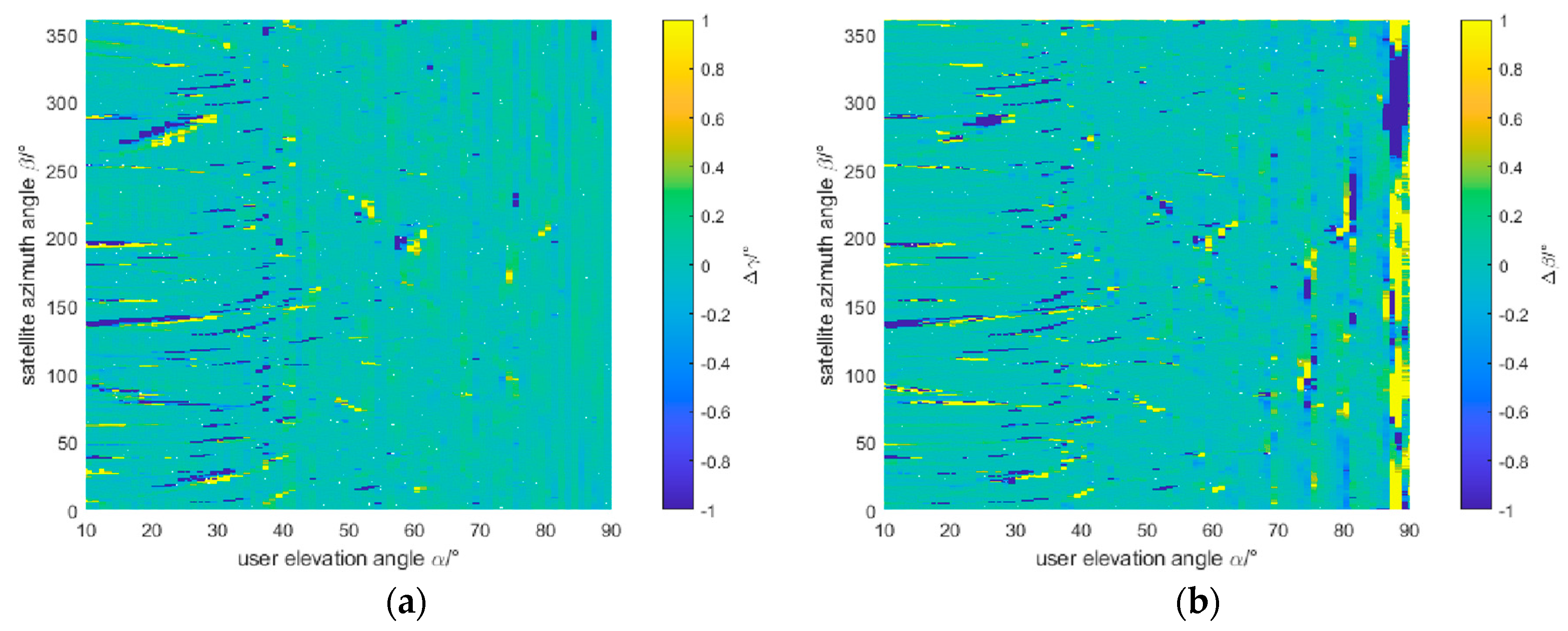
It is not difficult to see that when the user is at a low elevation angle, the error deviation and standard deviation of the satellite elevation angle and azimuth angle are generally large, and the convergence is not good. In addition, the azimuth angle also has a large deviation from the high user elevation angle, the standard deviation is generally greater than the general situation, and the data changes drastically, which may be due to the fact that the beam power difference of different users with high elevation angle is not obvious, and the solution of the azimuth angle has a certain impact.
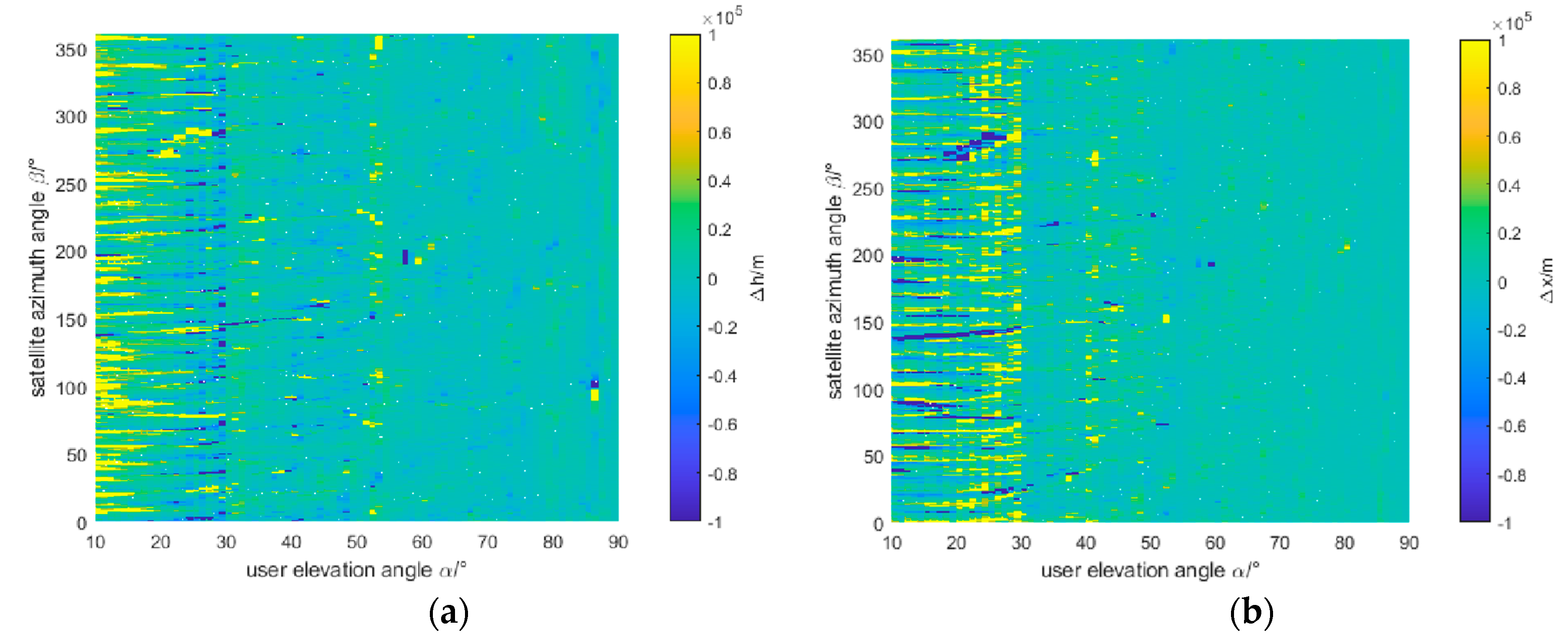
Figure 9.
(a)User vertical errors in different areas. (b) User horizontal errors in different areas.
Figure 9.
(a)User vertical errors in different areas. (b) User horizontal errors in different areas.
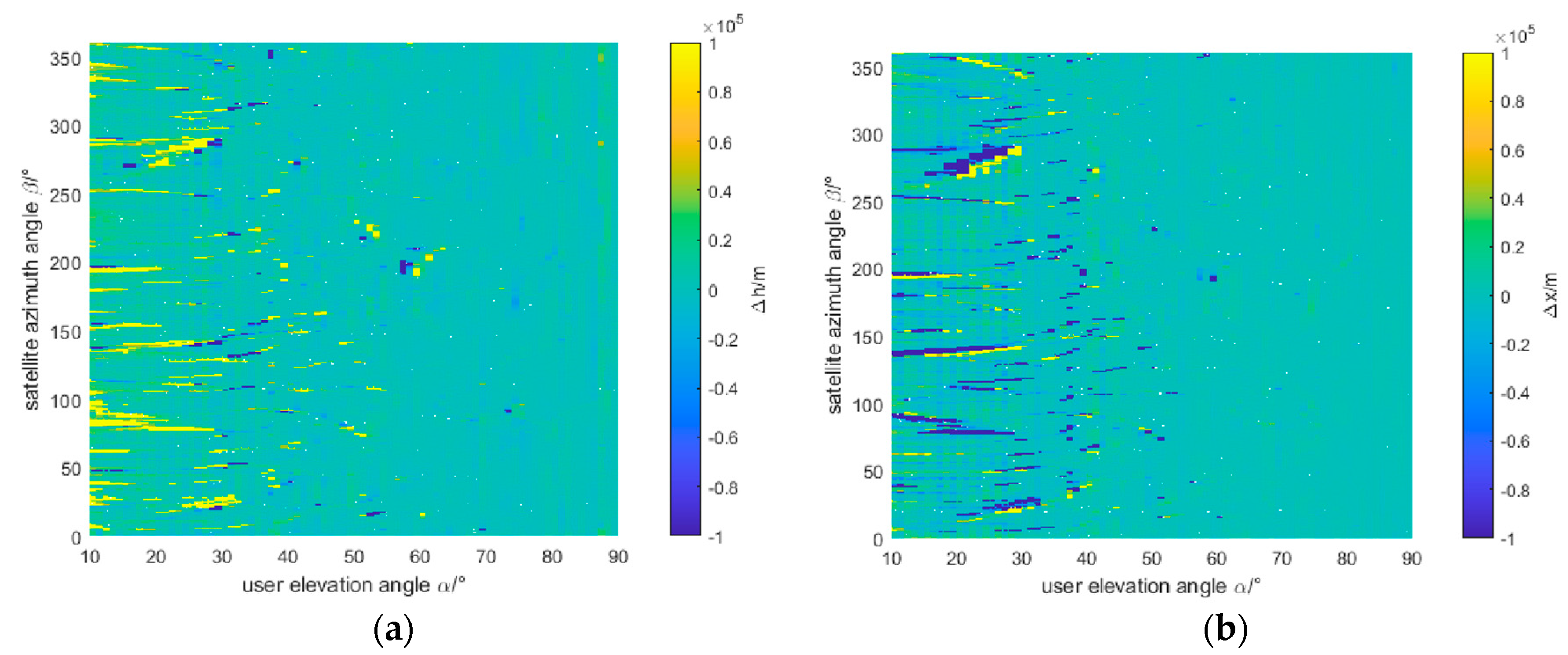
Figure 10.
Standard deviation of user horizontal errors in different areas.
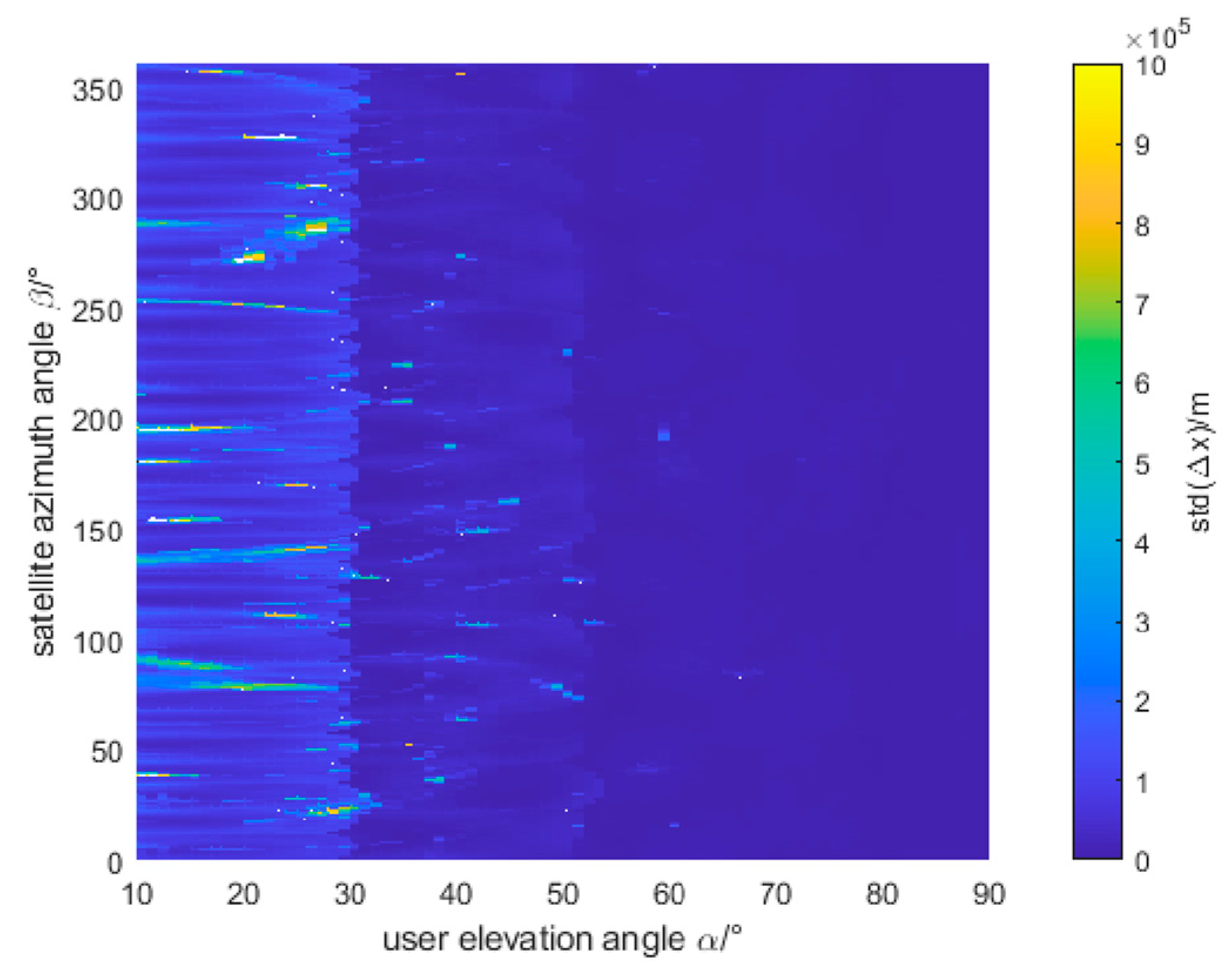
The solved user vertical and horizontal difference information exhibits properties similar to the errors in satellite elevation angles, with deviations generally being larger at low elevation angles and standard deviations also being larger at low elevation angles, with a clear stratification phenomenon observable: taking horizontal difference as an example, when the elevation angle is between 0° and 30°, the standard deviation is generally between 20-30km; when the elevation angle is between 30° and 50°, the standard deviation is generally between 10-20km; and when the elevation angle is greater than 50°, the standard deviation is generally less than 10km. This is because the calculation of user vertical and horizontal distance is tightly coupled with the satellite elevation angle, while the satellite azimuth angle is only used to determine the beam position and reverse link loss, thus having a less significant impact. The following results are obtained from the statistical analysis of user errors at different user elevation angles:
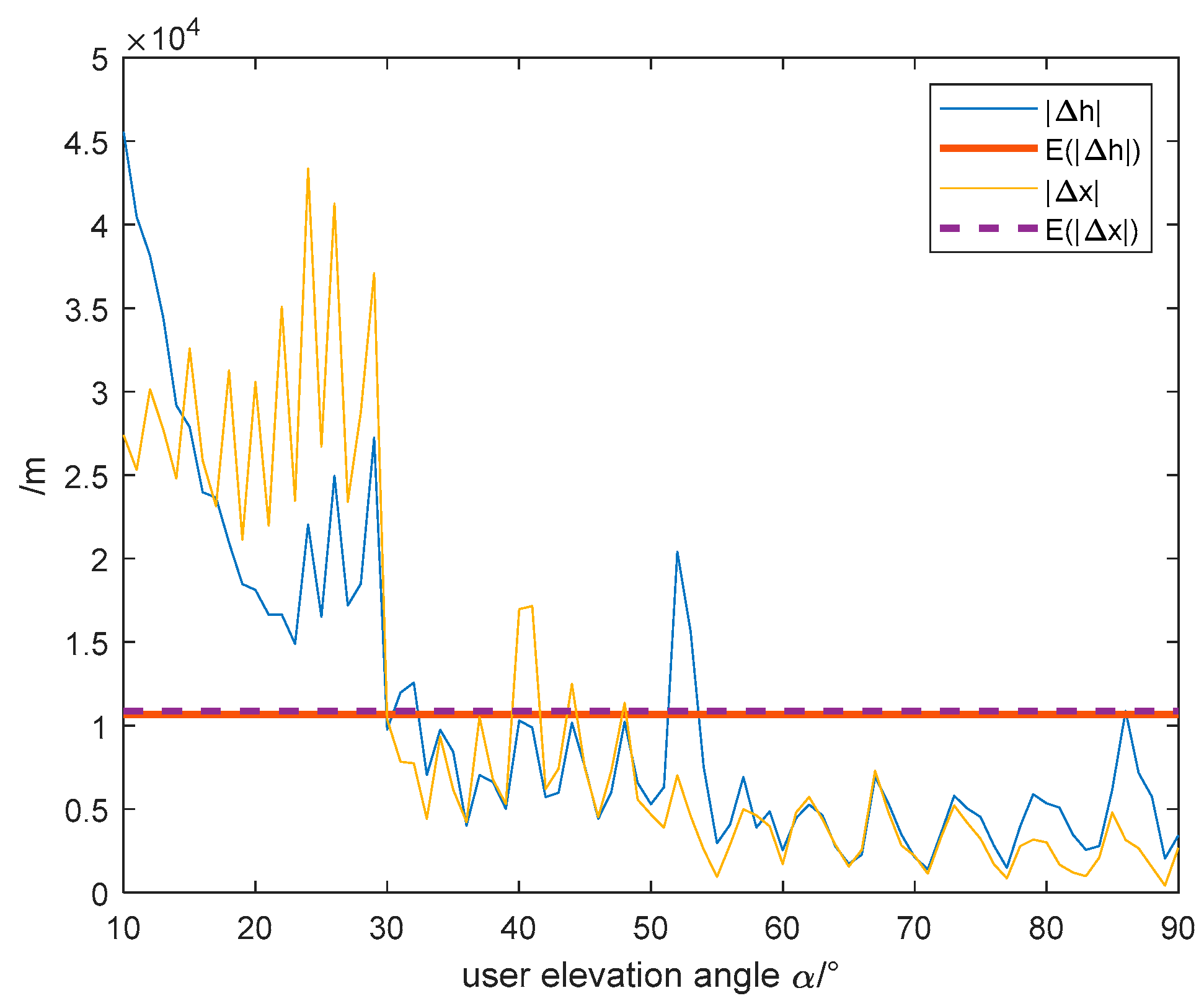
Figure 11.
Vertical and horizontal deviations of different user elevation angles.
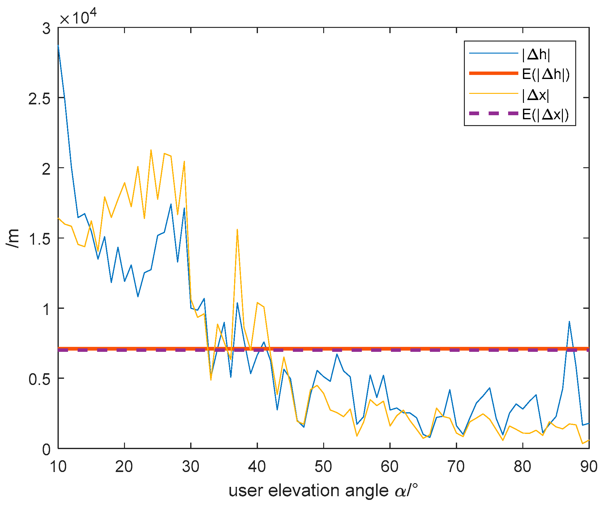
The numerical results of the aforementioned image can be further analyzed. First, by discussing the situation for all users, i.e., users with elevation angles , the overall performance of power positioning can be obtained. Then, by separately discussing the two major parts of low user elevation angles and high user elevation angles , the positioning and timing performance of users in different elevation angle regions can be obtained. The error table is as follows:
The power positioning timing error is affected by the user's position as follows:
Figure 12.
Timing errors of power positioning.
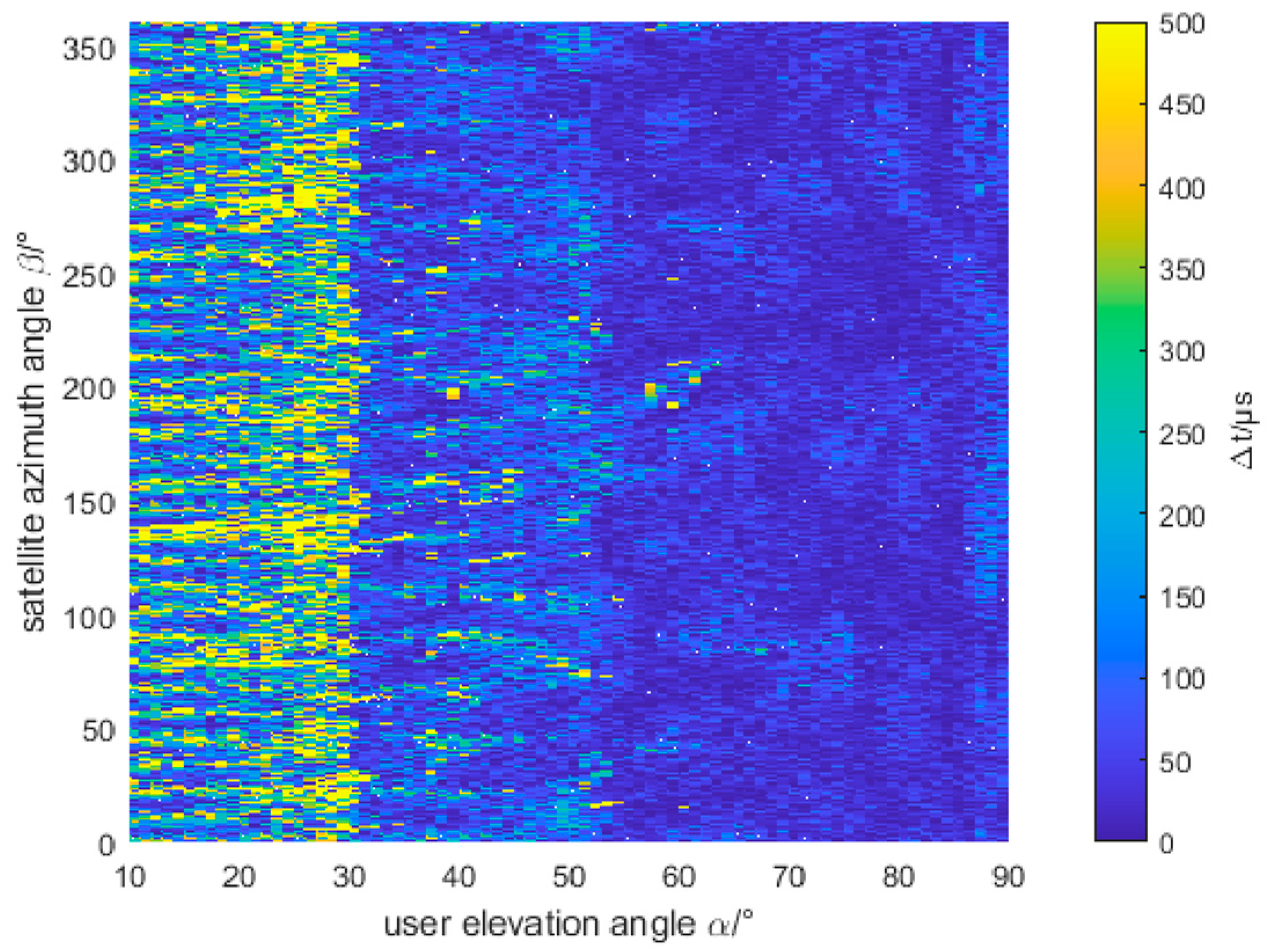
The maximum timing error is 10.1ms, and the statistical mean is 123μs. When the user's elevation angle is below 30°, the average timing error is 305.8μs; when the user's elevation angle is above 30°, the average timing error is 62.3μs. Therefore, power positioning can provide users with microsecond-level timing accuracy.
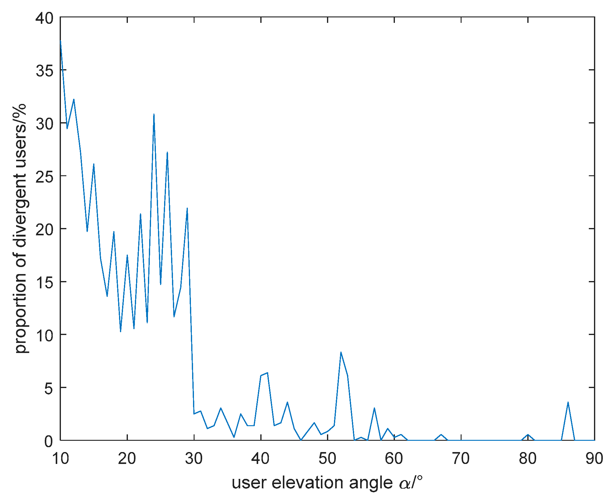
When the user's horizontal or vertical difference exceeds the convergence condition of 50km, the algorithm is judged to diverge, and the availability of power positioning is poor. By statistically analyzing the results for different user elevation angles, the positioning availability can be obtained as shown in the following figure:
Figure 13.
Usability of power positioning.
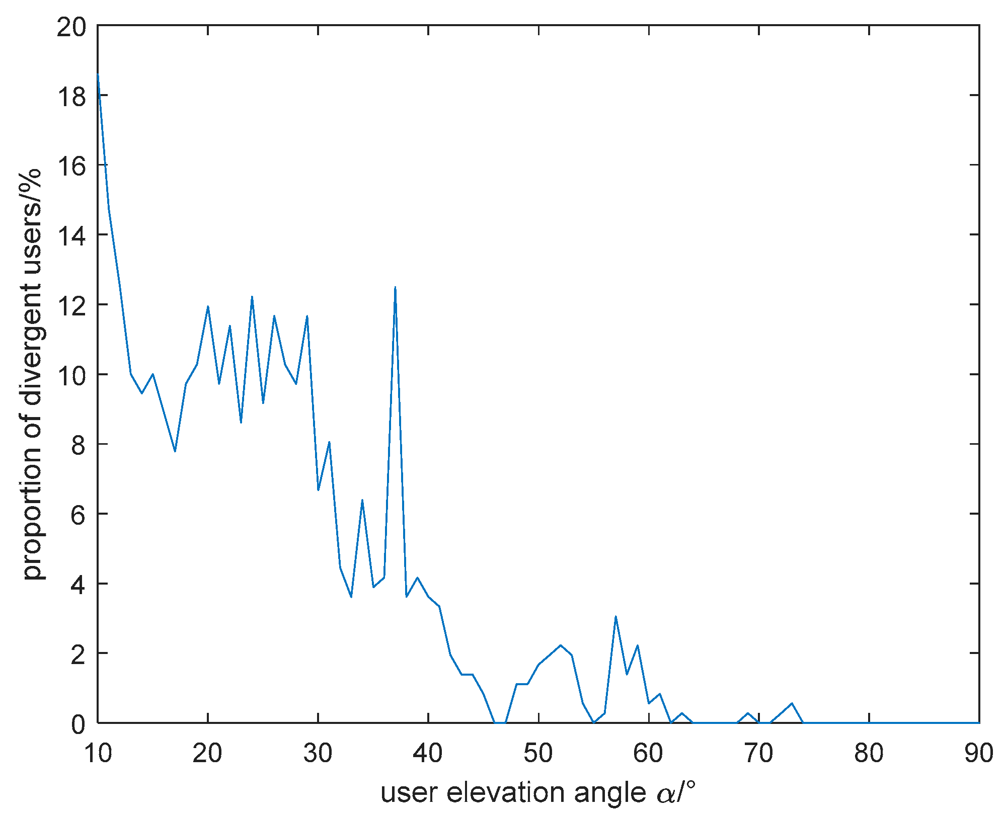
It can be seen that when the user's elevation angle is less than 30°, the proportion of divergent users is generally more than 10%, and the availability of power positioning is about 90%; when the elevation angle is greater than 30°, the proportion of divergent users is generally within 5% (users with an elevation angle of 37° are relatively special, related to the beam characteristics), and the availability of power positioning is above 95%. In summary, power positioning allows some users, especially those with high elevation angles, to have the potential to achieve better positioning and timing performance.
4.2. Received Power and Sensitivity
The simulation is set with a certain receiving power sensitivity threshold. When the received power exceeds this threshold, the power measurements are processed; otherwise, the power value is considered to be significantly affected by noise and is not subjected to least squares iteration processing. Previous simulations were all conducted under the condition of a threshold of -160dBm, which has high requirements for data quality. In this section, the receiver sensitivity is lowered to -190dBm to explore the impact of receiving power sensitivity on power positioning.
As with section 4.1, the angle conditions are as the same. However, the receiver sensitivity is set to -190dBm. The following two figures illustrate the impact of the user's elevation angle and azimuth angle on the vertical and horizontal error biases in power positioning:
Figure 14.
(a)User vertical errors in different areas when receiver sensitivity is -190 dBm. (b) User horizontal errors in different areas when receiver sensitivity is -190 dBm.
Figure 14.
(a)User vertical errors in different areas when receiver sensitivity is -190 dBm. (b) User horizontal errors in different areas when receiver sensitivity is -190 dBm.
It can be observed that when the user's elevation angle is low, for example, below 30°, the receiver with -190dBm sensitivity exhibits more divergence in power positioning compared to the receiver with -160dBm sensitivity. This indicates that while increasing the receiver sensitivity makes it easier to receive signals from different beams, the power positioning algorithm becomes more challenging to converge due to noise interference. Therefore, to enable more users to achieve better performance with power positioning, it is necessary to reduce the receiver sensitivity to a certain extent, in order to mitigate the impact of noise on the solution. As with subsection 4.1, by statistically analyzing the error biases for users with different elevation angles, the following results can be obtained:
Figure 15.
Vertical and horizontal deviations of different user elevation angles when receiver sensitivity is -190 dBm.
Figure 15.
Vertical and horizontal deviations of different user elevation angles when receiver sensitivity is -190 dBm.
The resulting error table is as follows:

Table 3.
Satellite and user error table when receiver sensitivity is -190 dBm.
| User elevation angle range | Evaluation criteria | /m | /m | ||
|---|---|---|---|---|---|
| [10,90] | deviation | 0.1349 | 0.2028 | 10650 | 10869 |
| std | 0.3724 | 0.6374 | 28955 | 33410 | |
| [10,30] | deviation | 0.1639 | 0.1556 | 24052 | 28155 |
| std | 0.5325 | 0.4881 | 65283 | 90783 | |
| [30,90] | deviation | 0.1239 | 0.2177 | 6022.1 | 4910.3 |
| std | 0.3174 | 0.6847 | 16740 | 13961 |
From the table, it can be seen that the standard deviations of user vertical difference and horizontal difference obtained by the high-sensitivity receiver are comparable to those under low-sensitivity conditions. However, the error biases of satellite elevation angle and satellite azimuth angle have increased by 0.0311° and 0.0789°, respectively, and the biases of user vertical and horizontal errors have increased by 3556.5m and 3859.7m, respectively. Under low user elevation angles, the biases of vertical difference and horizontal difference have increased by 8506m and 10975m, respectively, while under high user elevation angles, the biases have increased by 1790.9m and 1343.2m, respectively. It is not difficult to find that high sensitivity has a very significant impact on users with low elevation angles, while the impact on users with high elevation angles is relatively small.
Figure 16.
Usability of power positioning when receiver sensitivity is -190 dBm.
Statistical analysis of the availability for users with different elevation angles shows that when the user's receiving power sensitivity increases, users with low elevation angles are more severely affected by noise. When the elevation angle is below 30°, the proportion of users with divergent power positioning can be as high as over 30%, reducing the availability to 70%. The availability for users with high elevation angles can basically be maintained above 90%, but in this case, the positioning and timing errors are larger compared to low sensitivity.
5. Conclusions
In scenarios where the number of low Earth orbit (LEO) satellites in view is limited, pseudorange and carrier phase positioning are not available, and single-satellite Doppler positioning has poor applicability, ground users can utilize the received power measurements from different beams of LEO satellites to calculate their own position and time, thereby quickly obtaining positioning and timing results. Based on the multi-beam interrogation characteristics of LEO satellites, this paper employs the nearest neighbor algorithm for power matching to obtain convergent initial values and uses the least squares iteration to solve for the user's horizontal and vertical information. Experimental results show that the nearest neighbor algorithm can achieve initial values for satellite elevation and azimuth angles within 2° when the fingerprint library interval uncertainty is 5°; under the condition of initial values within 2°, the least squares solution can achieve convergence for the vast majority of users (94.5%, 93.2%).
For the least squares algorithm solution, multiple Monte Carlo simulation results indicate that the satellite elevation and azimuth angles, as well as user vertical and horizontal differences obtained from power positioning calculations, follow a normal distribution and have a good normal fitting relationship. There is a significant difference in power positioning results for users at different locations. For a receiver with -160dBm sensitivity, the statistical error biases for horizontal and vertical positioning are approximately 7000m, and the average timing error is 123μs. Users with low elevation angles (below 30°) generally have error biases higher than the average, at 15546m and 17180m respectively, with a timing error of 305.8μs, and power positioning availability of about 90%. In contrast, users with high elevation angles (above 30°) generally have error biases lower than the average, at 4231.2m and 3567.1m respectively, with a timing error of 62.3μs, and availability above 95%. Under high receiver sensitivity at -190dBm, affected by noise, the average error bias is about 10000m, with low elevation angle users being particularly affected, with an average bias worsening to over 20000m, and availability worsening to 70%. For high elevation angle users, the average bias only worsens to about 6000m, and power positioning availability is basically maintained above 90%.
In summary, the positioning accuracy of low Earth orbit multi-beam power positioning technology is at the kilometer level, and the timing accuracy is at the microsecond level, which can meet users' needs for real-time approximate position and time information.
References
- Yuanxi Yang; Yue Mao, et al. Demand and key technology for a LEO constellation as augmentation of satellite navigation systems. Satellite Navigation,2024, Vol.5(1): 1-9.
- Run Tian, Zhiying Cui, Shuangna Zhang, et al. Overview of the Development of Navigation Augmentation Technology Based on Low-orbit Communication Constellation. Navigation Positioning and Timing, 2021,8(1):66-81.
- Benzerrouk H, Nguyen Q, Fang X X, et al. 2019 26th Saint Petersburg International Conference on Integrated Navigation Systems (ICINS). St. Petersburg: IEEE,2019: 1.
- Xingxing Li; Yehao Zhao, et al. LEO real-time ambiguity-fixed precise orbit determination with onboard GPS/Galileo observations. GPS Solutions,2024, Vol.28(4).
- Morales-Ferre, R., Lohan, E. S., Falco, G., & Falletti, E. GDOP-based analysis of suitability of LEO constellations for future satellite-based positioning. In8th IEEE international conference on wireless for space and extreme environments (WiSEE), 2020, pp. 147–152.
- Psiaki, M. L. Navigation using carrier Doppler shift from a LEO constellation: TRANSIT on steroids. Navigation,2021,68(3), 621–641.
- Tan, Z., Qin, H., Cong, L., & Zhao, C. New method for positioning using Iridium satellite signals of opportunity. IEEE Access,2019, 7:83412–83423.
- Fei Guo; Yan Yang et al. Instantaneous velocity determination and positioning using Doppler shift from a LEO constellation. Satellite Navigation,2023.
- Sgammini, M., Cannas, A., Carchiolo, V., Giorgetti, G., & Veronesi, F. High-precision vehicular navigation using Doppler radars: A review and future directions. IEEE Transactions on Industrial Informatics,2019, 17(1), 345-362.
- Ju Hong; Rui Tu, et al. GNSS rapid precise point positioning enhanced by low Earth orbit satellites. Satellite Navigation,2023, Vol.4(1): 1-13.
- Chuang Shi; Yulu Zhang, et al. Revisiting Doppler positioning performance with LEO satellites. GPS Solutions,2023, Vol.27(3).
- Jingxue Bi; Yunjia Wang, et al. Supplementary open dataset for WiFi indoor localization based on received signal strength [J]. Satellite Navigation,2022, Vol.3(1): 1-15.
- KAN C, DING G, WU Q, et al. Robust Relative Fingerprinting-Based Passive Source Localization via Data Cleansing [J]. IEEE Access,2018,6:19295-19269.
- Kaemarungsi, K., & Krishnamurthy, P. Modeling of indoor positioning systemsbased on location fingerprinting. In IEEE INFOCOM 2004, Vol. 2, pp. 1012–1022.
- Li, J., Gao, X., Hu, Z., et al. Indoor localization method based on regional division with IFCM. Electronics, 2019,8(5), 559.
- Feng, Y., Minghua, J., Jing, L., Xiao, Q., Ming, H., Tao, P., & Xinrong, H. Improved AdaBoost-based fingerprint algorithm for WiFi indoor localization. In 2014 IEEE 7th joint international information technology and artificial intelligence conference,2014, pp. 16–19.
- Li, Y., et al.Toward location-enabled IoT (LE-IoT): IoT positioning techniques, error sources, and error mitigation. IEEE Internet of Things Journal,2021,8(6), 4035–4062.
- Chen, G., Meng, X., Wang, Y., Zhang, Y., Tian, P., & Yang, H.Integrated WiFi/PDR/smartphone using an unscented Kalman filter algorithm for 3d indoor localization. Sensors,2015,15, 24595–24614.
- Bi, J., Wang, Y., Li, X., Cao, H., Qi, H., & Wang, Y. A novel method of adaptive weighted K-nearest neighbor fingerprint indoor positioning considering user’s orientation. International Journal of Distributed Sensor Networks,2018.
- Deng, Z., Fan, J., & Jiao, J. D-SVM fusion clustering algorithm based on indoor location.2018.
Figure 1.
Geometry of the user's received satellite signal.
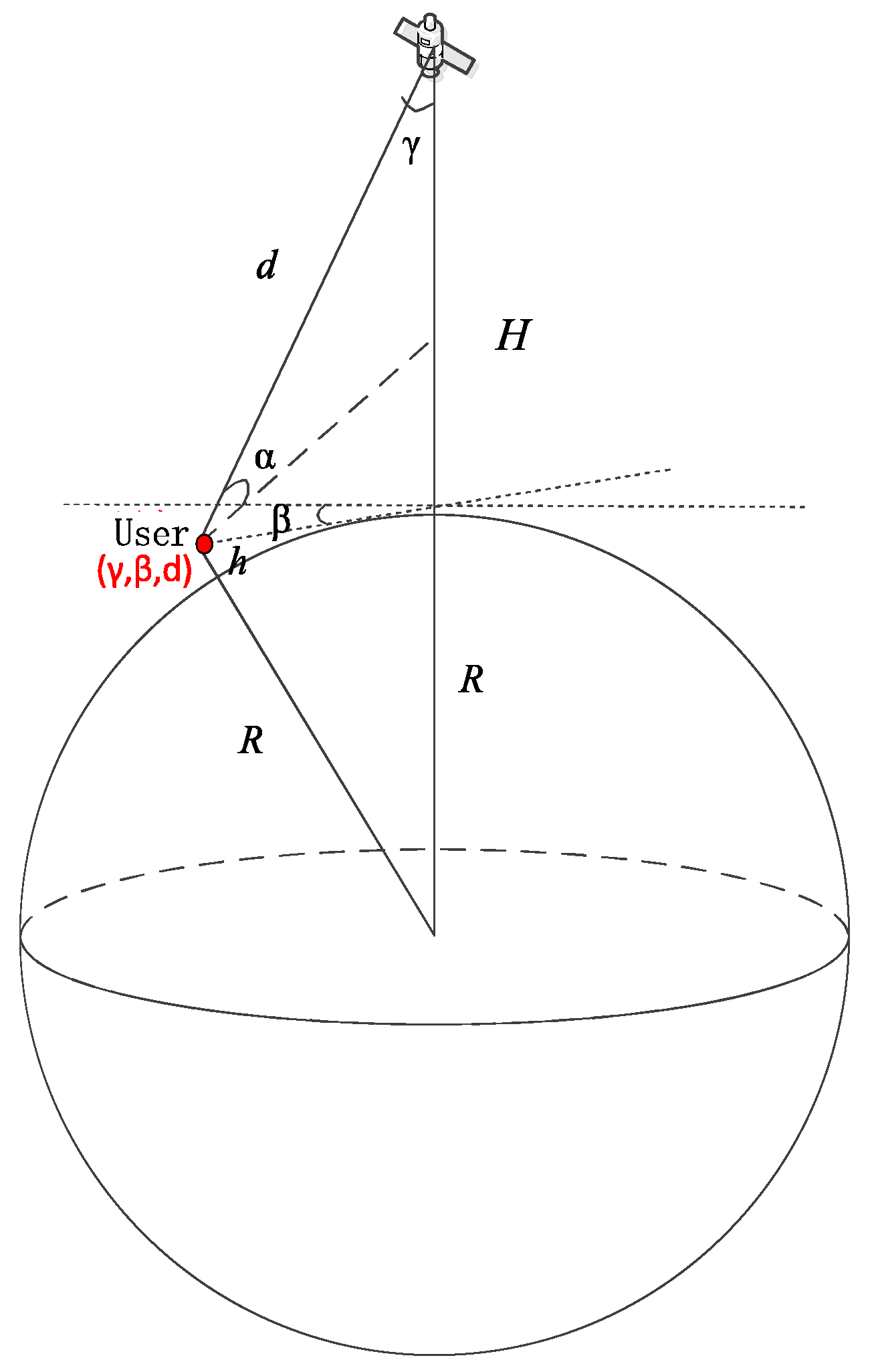
Figure 2.
Flowchart of the power positioning least squares algorithm.
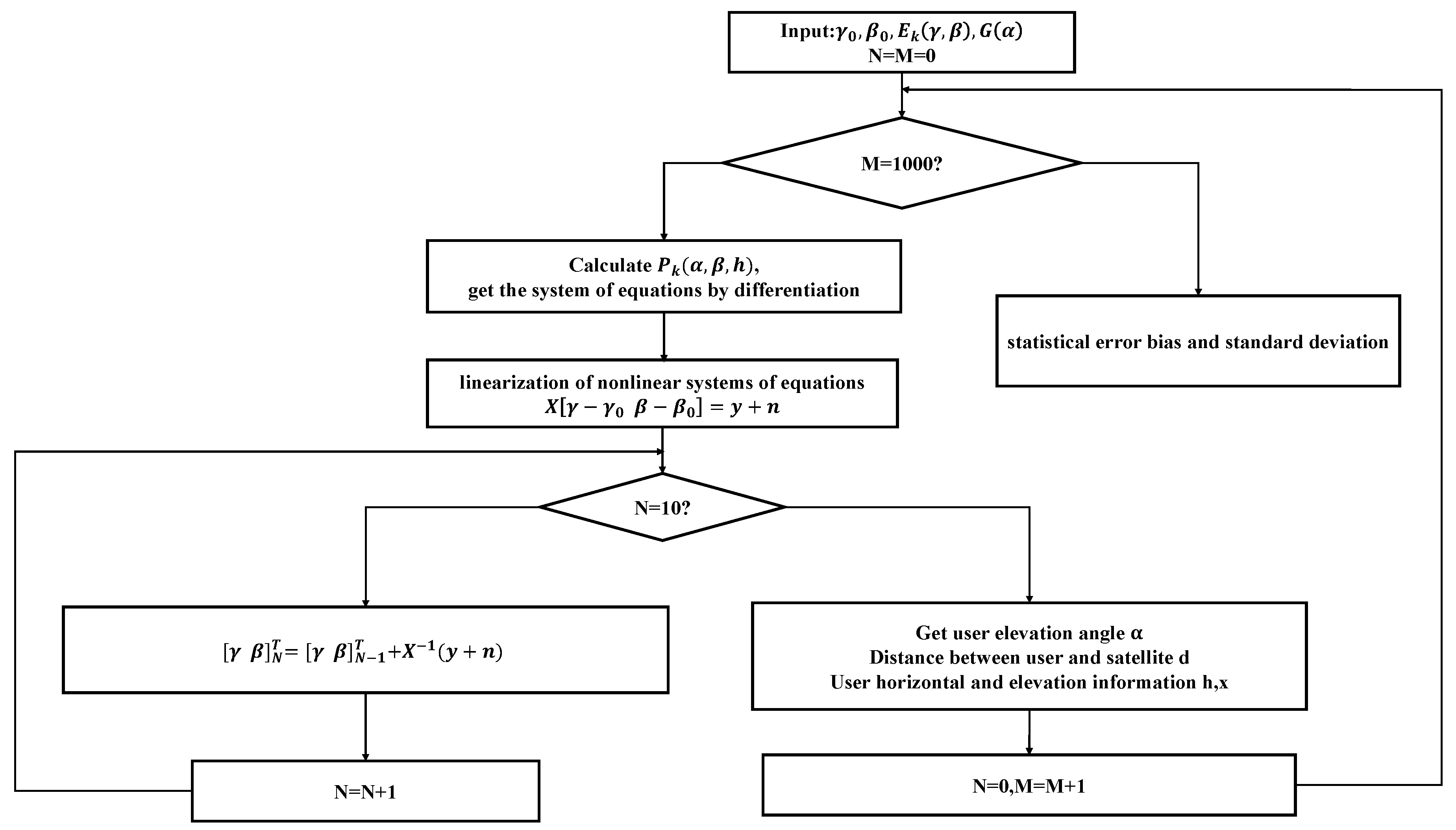
Figure 3.
Convergent and divergent solutions of the least squares algorithm.
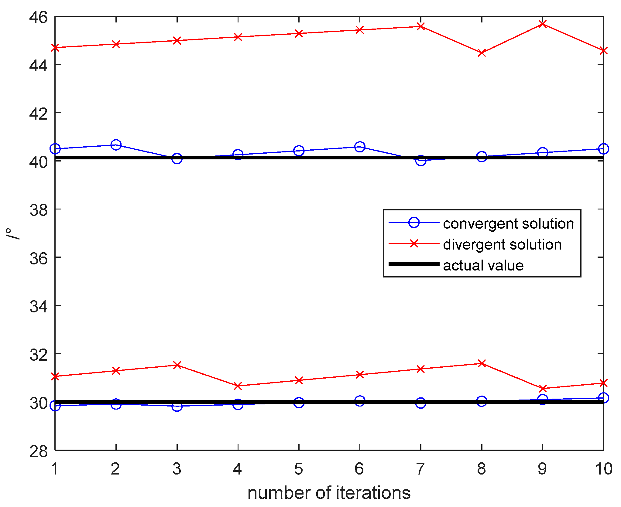
Figure 4.
Initial value requirements for satellite elevation and azimuth angles.
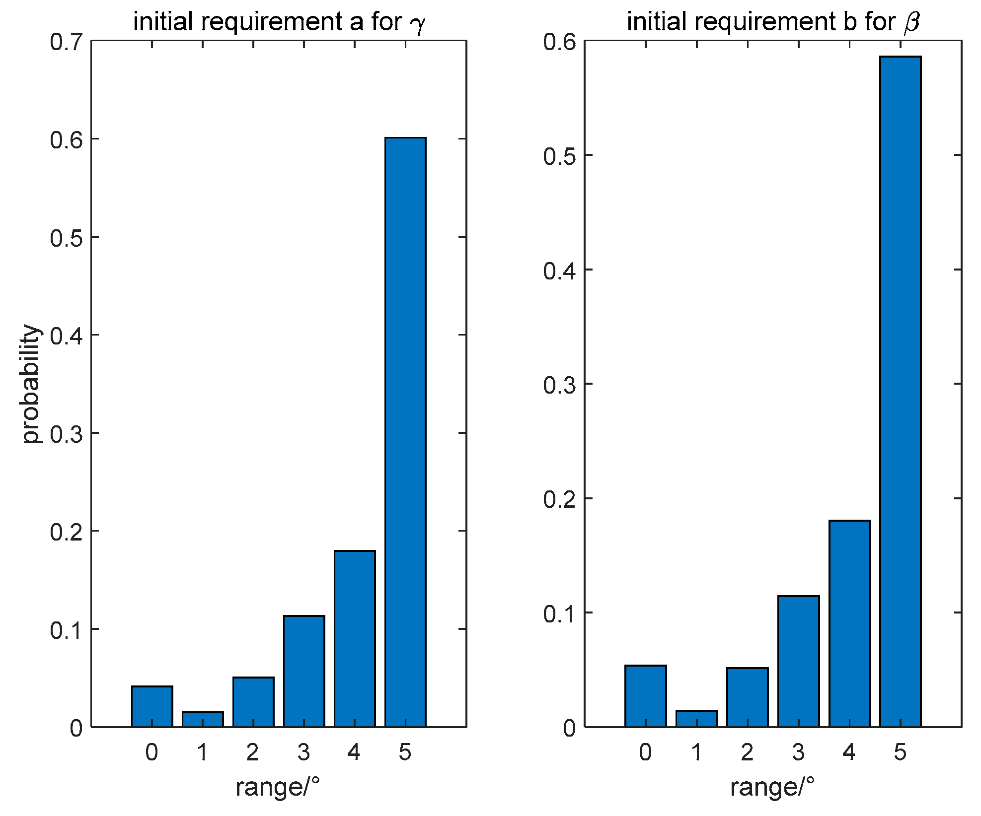
Figure 5.
(a) Satellite elevation angle error of nearest neighbor algorithm. (b) Satellite azimuth angle error of nearest neighbor algorithm.
Figure 5.
(a) Satellite elevation angle error of nearest neighbor algorithm. (b) Satellite azimuth angle error of nearest neighbor algorithm.
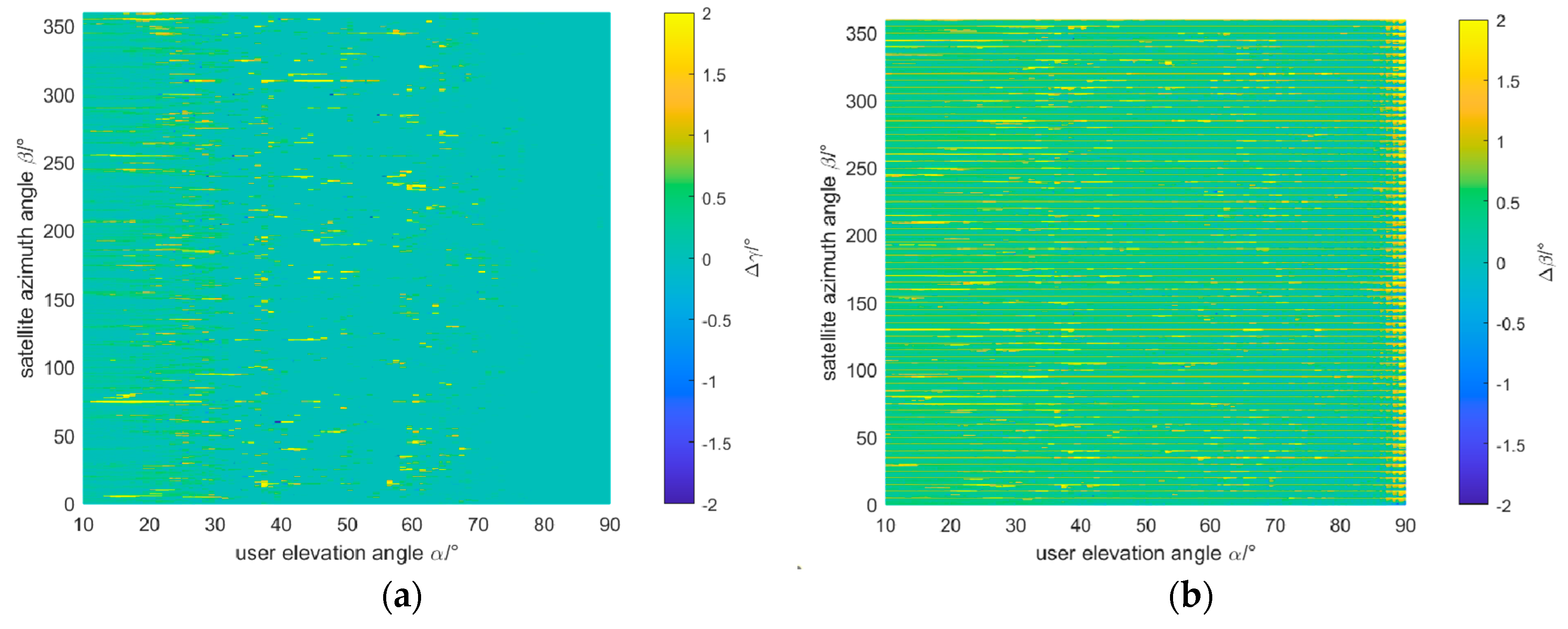
Figure 6.
Monte Carlo results of .
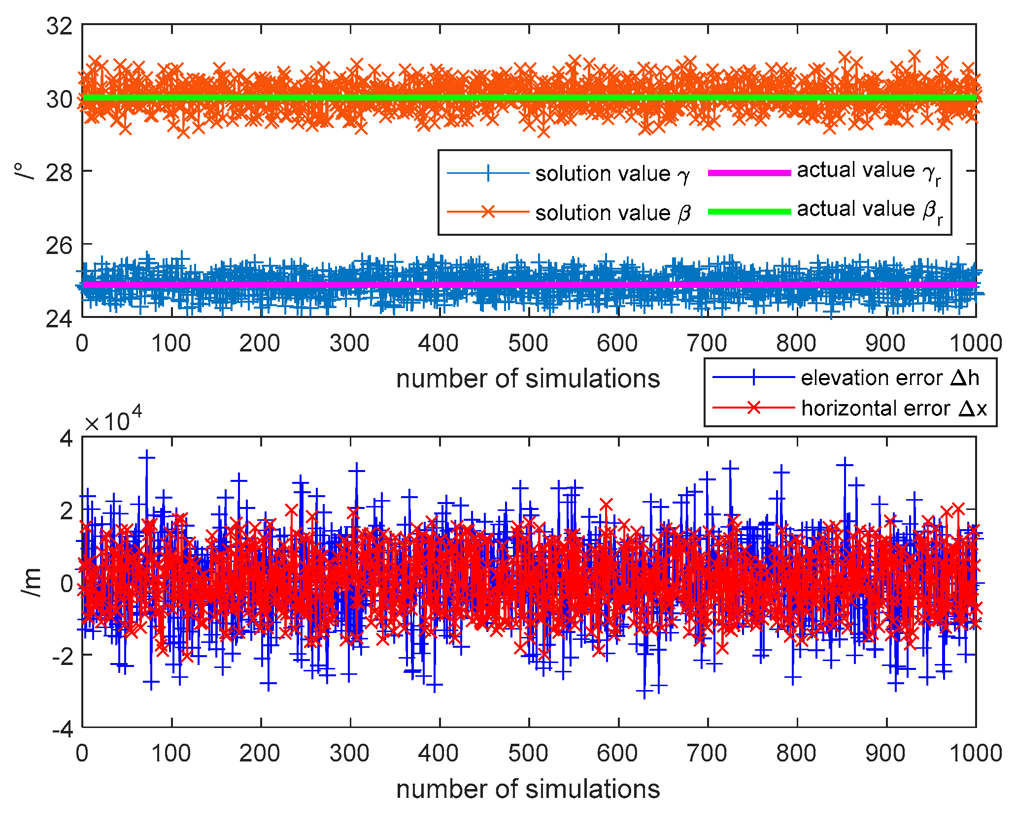
Figure 7.
Normal distribution fits of Monte Carlo results.
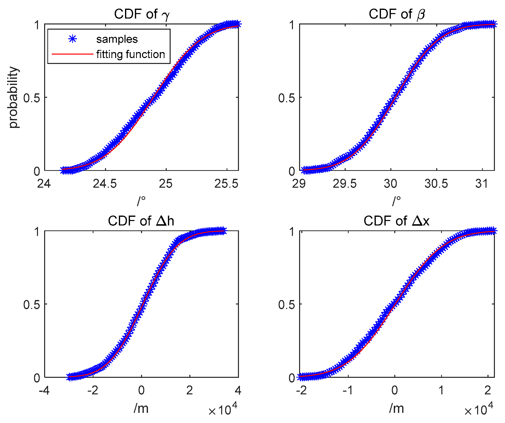
Table 1.
Simulation parameters.
| Parameter type | Parameter value |
| Earth radius | 6371km |
| Satellite orbital altitude | 1200km |
| User elevation angle | [10,90] |
| Satellite elevation angle | can be calculated by |
| satellite azimuth angle | [,360] |
| Total number of satellite beams | 52 |
| User geodetic height | 0m |
| User gain | 0dB |
| Noise bandwidth | 1000Hz |
| Noise temperature | 290K |
| Least squares iterations | 10 |
| Number of power fingerprint bank beams | 10 |
| Receiver sensitivity | -160dBm, -190dBm |
Table 2.
Satellite and user error table when receiver sensitivity is -160dBm.
| User elevation angle range | Evaluation criteria | /m | /m | ||
|---|---|---|---|---|---|
| [10,90] | deviation | 0.1038 | 0.1239 | 7093.5 | 7009.3 |
| std | 0.5016 | 1.1811 | 31720 | 53403 | |
| [10,30] | deviation | 0.1683 | 0.0996 | 15546 | 17180 |
| std | 0.9562 | 1.9617 | 74503 | 165260 | |
| [30,90] | deviation | 0.0817 | 0.1316 | 4231.2 | 3567.1 |
| std | 0.3455 | 0.8340 | 17385 | 15062 |
Disclaimer/Publisher’s Note: The statements, opinions and data contained in all publications are solely those of the individual author(s) and contributor(s) and not of MDPI and/or the editor(s). MDPI and/or the editor(s) disclaim responsibility for any injury to people or property resulting from any ideas, methods, instructions or products referred to in the content. |
© 2024 by the authors. Licensee MDPI, Basel, Switzerland. This article is an open access article distributed under the terms and conditions of the Creative Commons Attribution (CC BY) license (http://creativecommons.org/licenses/by/4.0/).
Copyright: This open access article is published under a Creative Commons CC BY 4.0 license, which permit the free download, distribution, and reuse, provided that the author and preprint are cited in any reuse.


