Submitted:
03 January 2025
Posted:
03 January 2025
You are already at the latest version
Abstract
Terrestrial and satellite communications, tactical data links, positioning, navigation, and timing (PNT), and distributed sensing will continue requiring precision timing and the ability to synchronize and disseminate time. However, as the supply of space-qualified clocks with Global Navigation Satellite Systems (GNSS)-level performance is limited and the understanding of disruptions to GNSS due to potential adversarial actions increases, the current practice of reliance on the GNSS-level timing becomes costly and outdated when compared with an on-orbit assembly of robust and stable timescale references, especially being considered as the development of diverse alternatives to GNSS. Onboard realization of clock ensembles is particularly attractive for applications such as on-demand dissemination of GPS Time (GPST) like navigation services via a proliferated Low-Earth-Orbit (pLEO) constellation. This article investigates the overarching goal of agility and reprogrammability, where rate-based linear quadratic regulators for both communication and clock data transfer services are proposed to flexibly allocate radio resources away from primary communication services to clock data transfer services for on-demand pLEOT formations within pLEO constellations. Next, the work here is proposing the model-based control of wireless networked timing systems. It embraces the vision of optimally placing critical information of the implicit ensemble mean (IEM) estimation about the multi-platform clock ensemble that has better stability than any individual member of the ensemble on the network to flexibly reduce the data traffic. By making the remote sensor of IEM estimates running onboard the anchor platform and actuators for optimal steering of remote frequency standards located at participating platforms more "intelligent" that supports onboard IEM timescale realizations across a pLEO constellation, the networked control system can predict future behaviors of local reference clocks accompanied with low-noise oscillators and then send precise information on the IEM estimation at critical times to ensure the realization of a common pLEO timescale onboard all participating platforms. Clock steering is especially essential for the realization of timescales. Performance realizations are generally dependent on the control intervals and steering techniques chosen. Towards performance robustness beyond what the existing steering technique of Linear Quadratic Gaussian control can offer, the minimal-cost-variance (MCV) steering paradigm is proposed from the perspective of minimizing the variance of the integral-quadratic-form performance measure of the Linear Quadratic Gaussian control subject to a constraint on its mean.
Keywords:
Proliferated Low-Earth-Orbit Constellation
; Integrated Communication and Navigation
; Clock-to-Clock Difference Measurements
; Multi-Platform Clock Ensemble
; Clock Ensemble Kalman Filter
; Implicit Ensemble Mean
; Networked Control System
; Minimal Attention Control
; Minium-Cost-Variance Clock Steering
; Linear Quadratic Regulators
1. Introduction
The rapid development of pLEO constellations of small satellites has greatly provided communications and navigation services [1,2], and [3]. These recent studies suggest that the global coverage provided by these pLEO constellations brings unprecedented opportunities for alternative positioning, navigation, and timing (AltPNT) solutions. According to GNSS, one-way time-of-flight-based navigation services require close monitoring of stable clocks, from which ranging signals are generated. Moreover, multiple, highly stable, microwave clocks onboard each satellite are further integrated with a time-keeping system. Both aspects of overcoming the behavior of satellite clocks and assembling with laboratory-based clocks to produce a timescale are paramount to tracking GNSS signals from ground reference stations around the world and the corrections for each satellite clock concerning the reference timescale distributed to users [4,5], and [6].
Note that the principles behind the concept of operations for GNSS, including large and heavy clocks onboard each satellite, monitoring them from the ground, and uploading clock corrections to each satellite for distribution to the user segment, are not suitable for smaller LEO spacecraft with much shorter orbital lifetimes. However, observing each onboard clock in the pLEO constellation requires extensive tasking responsibilities from the ground-monitoring network due to the need for a global navigation service from LEO regimes. To efficiently tackle the first challenge, the foundation of the underlying GNSS timescales must be rethought from scratch. The assembly of multiple low-size, weight, and power (SWaP) clocks appears more suitable than a single high-performance clock. As for the second challenge, a new conformance framework for seamless realizations and interactions of composable and reference timescales is needed in a distributed architecture.
To this end, one of the promising paths to address the issues mentioned earlier is to adopt two-way time and frequency transfers between pLEO platforms, which facilitate the use of low SWaP clocks without resorting to large-scale ground monitoring and/or GNSS availability. Such a concept will prove to be essential to leveraging the extensive connectivity among the platforms already in place for various primary data transport applications [7] and [8]. As expected, radio frequency antenna and onboard terminals equipped on each pLEO platform will provide in-plane and cross-plane connections [9]. In particular, the use of networks consisting of inter-satellite links as a media to interconnect the different pLEO platforms enables data transports, ranging measurements, and clock comparisons. It is clear that by relying on inter-satellite links, the realization of clock comparisons among small atomic clocks onboard each pLEO satellite offers potential reductions of ground monitoring requirements, allowing differential clock phase measurements to be directly input into clock ensembling algorithms [10]. Such a capability becomes critical to supporting the on-demand generation of local realizations of pLEO time (pLEOT), i.e., a constellation timescale analogous to Global Positioning Systems time or GPST.
This article is organized as follows. As discussed in Section 2, it turns out that the control engineering principles would provide answers to the fundamental question of how each participating pLEO platform could meet ad-hoc clock data transfer requests, by promoting autonomy increase in reprogrammability for integrated broadcasting signals for integrity, robustness, and security expected. Section 3 describes a pLEO timescale concept, including its critical clock dynamics and frequency standards of the varying types of participant low SWaP clocks, in an attempt to create an autonomous and robust pLEO timescale that may be capable of becoming Master Clock reference signals should the need arise. It explores a networked clock system of a finite number of free-running clocks onboard cooperating pLEO platforms and related by clock-to-clock difference measurements. Clock difference measurements are then coordinated by multi-way time transfer and synchronization. In Section 4, the implicit ensemble mean (IEM) estimation is proven to be indispensable when forming a paper clock running onboard an anchor platform within the pLEO constellation. Every corrected clocked in the pLEO constellation can now represent the IEM as accurately as possible. As shown in Section 5, the concept of synchronization of satellites within the pLEO constellation with the pLEOT requires a real clock onboard each platform to be steered against the paper clock for the realization of the composite clock. Consequently, network update rates with distributed IEM information are essential to steering commands with minimal attention for an IEM realization. Section 6 introduces a novel clock steering technique based on the MCV control theory, which can lead to a better understanding of stochastic control for autonomous realizations of the IEM timescale onboard each separate platform with higher performance and robustness in stochastic clock anomalies. Lastly, Section 7 offers some remarks and conclusions.
2. Concept of Operations
An example illustration of the future concept of PNT over communications operations for asynchronous interactions between ad-hoc non-dedicated pLEOT formations and primary radio communication services within a pLEO constellation is considered in Figure 1, where incumbent orbital assets are capable of transmitting additional ad-hoc non-dedicated clock data services, e.g., free-running clock states, clock difference observables, IEM estimates, etc. during a window when the pLEOT service must occur. As depicted in Figure 1, all the free-running clocks onboard participating assets serve as the clock ensemble and are used to generate the clock ensemble timescale. At the window of pLEOT generation, member clocks together with their signal generations are measured against one another via non-dedicated inter-satellite radio links and inter-platform time transfer and synchronization protocols. Then the clock-to-clock difference measurements are fed into a clock ensemble Kalman filter running onboard an anchor asset of choice. Finally, the filter estimates every ensemble clock and distributes signal generation components necessary for onboard pLEOT timescale formations onboard participating assets while subject to the underlying crosslink network constraints.
2.1. Integrated Broadcasting Signal Structure
With a limited communication capacity from any given pLEO platform i and , a non-dedicated and low-power signal for coordinating clock comparisons and ensemble clock estimates is added to its primary and existing communication missions. It is assumed that both no-dedicated clock and primary communication data are spread by different spreading pseudo-random-number (PRN) sequences orthogonal to each other. The two kinds of signals are then transmitted synchronously with the same frequency and phase on crosslinks, e.g.,
where an on-demand pLEOT service horizon T is discretized to some constant quanta of the size , e.g., minute and each unit of represents one time step k.
As depicted in (1), the method of signal integration herein is primarily characterized by three properties: the low-latency yet discreet physical-layer approach that embeds the clock signal onto the existing communication signal without requiring additional bandwidth and power resources; radio backward compatibility where existing communication receivers and remote timing systems in service could still maintain their respective functions without any modifications; and the same radio frequency and different PRN sequences that leverage the radio frequency circuits of traditional communication receivers.
2.2. CN0 of Clock and Communication Data Signals
Power spectral density of the signal generated by the method considered herein is illustrated in Figure 2. The characterization of the ICaC performance of an on-demand and non-dedicated pLEOT formation is captured in the detailed analysis of carrier power to noise power spectral density ratio (CN0) margins, communication capacity, etc.
An available integrated clock and communication (ICaC) signal from orbital platform i can be detected with sufficient strength to form usable measurements, i.e., CN0 threshold value required to acquire and track the signal and with unobstructed line of sight. For any duration of availability, the clock-to-interference-plus-noise ratio (CIR) of associated with connecting platform i is one of the primary drivers in clock data transfer performance, i.e.,
where and respectively are the powers of the clock and communication signals at the time instant . Also relevant are the total bandwidth and double-sided noise power-spectral density .
Of note, the primary communication signal is jamming the non-dedicated clock signal with relatively high power. As shown in (2), however, both characteristics of very low signal power and very large processing gain from direct sequence spread spectrum characteristics are exploited here. Put differently, the communication signal is effectively treated as white noise and its power is the same as the power in the total band. Consequently, the interference caused by the communication signal is now much weaker than the background noise . Thus, the transmission of communication signals may be designed with minimal impacts on the clock data counterpart.
Due to the different design requirements, any ICaC signaling system onboard participating orbital platform i must compromise between two communication and clock data transfer aspects, or be more focused on one of them. For example, the communications-to-noise ratio (CNR) of that follows, can be interpreted as a measure of performance that communication services can expect while enabling non-dedicated clock data transfers in pLEOT realization, e.g.,
Based on the analysis shown (2) and (3), tradeoffs and interactions between CN0 values associated with communication and clock data services are used to determine the performance of non-dedicated clock data transfer service running onboard platform i, i.e.,
and
where in total, the parametric variable CN0 of clock and communication data should be chosen optimally for the performance of non-dedicated clock data transfers and primary communication services with certain qualities of services.
2.3. Robustness and Integrity
As an early initiative towards building low-latency and discreet clock data transfer, the paradigm shift in the non-dedicated pLEOT timescale for programmability and flexibility involves provisioning communication and clock radio resources and superimposing both communication and clock signal energies. The challenge of achieving the properties of integrity, robustness, and security of the ICaC signal as described in (1) requires appropriate power allocations in such a way the proposed ICaC paradigm is transparent and unobtrusive to unaware orbital platform equipment.
To achieve deep integration of communication and clock radio functions at the physical layer, local agent i residing at the ith-orbital platform asset in the non-dedicated pLEOT constellation will take independent and autonomous actions in reacting to transient power allocations of communication and clock data transfer requirements. In the framework of dynamic power allocation based on integral control considered hereafter, the allocated powers and for both communication and clock data transfer services at time instant is adjusted in proportion to the current shares and together with the amounts of adjustments and for communications rates and clock accuracy levels
provided that and for .
Similarly, it follows that
where and is the total power available at the ith-orbital platform.
In light of (6) and (7), it is conceivable that received signal powers can be adapted for communication and clock data service solutions. The adaptation of interoperable CN0 at the ith-orbital platform is given by
and
where is the rate of the total power of the ith-orbital platform. Needless to say, it is easy to realize that and are important parameters for integrity and robustness, which lead to robust communications with sufficient CNR and unobtrusive clock data transfers with appropriate CIR, respectively.
2.3.1. Robustness
One fundamental prerequisite toward realizing ICaC is the feasibility analysis. To this end, the appropriate power allocation is translated into a nonlinear tracking problem that achieves the desired signal-to-noise ratio, for the clock data transfer service. It can be cast into a linear power reference tracking by a suitable selection of the error function; i.e.,
In view of (4), one can obtain
where in fact, the power allocation associated with the clock data transfer service is employed to emulate a time-varying virtual power reference to achieve the desired ; i.e.,
Note that there is a fundamental tradeoff between robustness and integrity. When the paradigm is made more robust by increasing the value of the virtual power reference (13), it gives rise to the power of communication services and thus, impacts unaware clock data receivers.
2.3.2. Integrity
For integrated communication and pLEOT services, non-dedicated clock data signals become interferences to the existing communication counterparts. They would likely decrease the bit-error-rate (BER) performance. Henceforth, the power of clock data signals should be limited to guarantee the BER performance requirement. With that said, ameliorative approaches include efforts to unobtrusively place clock data signals within a family of noise distributions with unknown parameters that must be estimated by communication receivers. In this work, the non-dedicated clock data service is provisioned as the class of Gaussian distributed signals. Therefore, clock data signals would thus be observed in additive white Gaussian noises. According to the result (4), the communication receiver tests to see if the observation is Gaussian or not. If the CIR of as shown in (4) is kept at a certain threshold, namely , then the observed cumulative distribution function becomes indistinguishable from the normal distribution.
Progress in establishing programmability and flexibility for integrated communication and pLEOT services is much dependent on the success of the feedback loop in achieving the minimum unobtrusive guarantee. It is further contingent on the feasibility of the steady-state errors that describe the explicit relationship between the current CNR of and the desired unobtrusive threshold of , e.g.,
In the light of (8), it follows that the increment of , i.e., for communications can effectively affect the transient behavior of (15)
Consequently, an integrator of the errors as governed by (15) is added to the integral control-based CN0 allocation by the local agent i at the jth-orbital platform to eliminate potential steady-state errors; e.g.,
Note that the selection of highlights the requirement for pLEOT information that is distributed as noises. The emphasis, however, is still on non-dedicated clock data with low-power CN0 that accounts for small impacts on uninformed or unaware primary communication receivers.
2.4. Local Rate Regulators for Communications and Clock Data Services
What follows is a flexible framework of control autonomy for maintaining spread spectrum gains and multiple access performance of the family of physical-layer communication and pLEOT integration. Practically, only pertinent yet locally available information associated with the ith-orbital platform, including , , , and are required to make adaptive CN0 allocations for communication and pLEOT on ad-hoc non-dedicated demands.
Each local agent i has a periodic opportunity to compute increment policies pertaining to the total CN0 for integrated communication and clock data transfer services at the orbital platform i. Notwithstanding the main appeal of the difference equations as governed by (8), (9), (14), (16), and (17) makes them as a useful physical modeling tool to develop a discrete-time state-space model whose dynamics to be controlled are QoS satisfaction of communication and pLEOT services, i.e.,
With reference to the developed model, the aggregate state and control input vectors and the correspondent matrix coefficients of (18) are defined as follows
then the linear time-invariant state-space model (18) as demonstrated in Figure 3 enables the advantage of using the control engineering framework for CN0-based on-demand procedures at local agents, i.e.,
where in this case, the output coefficient is an identity matrix of size 6 and the feedthrough or feedforward is a zero matrix.
In CN0-based control protocols, the objective associated with local agent i is to drive increments of the total CN0 to desirable regulatory and reference tracking. Admittedly, it should be noted that total power of communications and clock data transfers is scarce. Oftentimes, the total CN0 resource might be over-provisioned. Special cares are needed to remain the balance of accuracy and CN0 margins, where CN0 margins are the differences between the CN0 of communications and clock data transfers in the integrated signal system and those of normal satellite communications and AltPNT. In addition, the utilization efficiency is considered by means of the constraint.
where both and are the 1st and 2nd-vector components of the distributed system state vector at time instant k.
2.4.1. Performance Specifications
The novelty of the work herein is that the analysis of control performance explicitly deals with dynamical variations of both communication and pLET realization requirements and effectively adapts the increments of the total CN0 available at the ith-orbital platform. In particular, the scenario considered in this work consists of the participation nature of the subsystems (8) and (9) subject to the constraint (21) while guaranteeing a satisfactory performance of minimal transient and steady-state errors as described in (14), (16), and (17).
In this regard, each local agent i autonomously assigns an optimal decision sequence of resource sharing , such that the performance index governed by the quadratic cost function that follows, is minimized over an infinite optimization horizon.
where denotes an initial system state whereas and are respectively symmetric, positive semi-definite and positive definite weighting matrices representing the degrees of freedom; e.g., , , , , , and
Through an appropriate selection of and parameters, the stable closed-loop system (19)-(20) can be guaranteed. Note that when the first quadratic term of (22) is small, most of the transient errors in tracking of desired CIR and CNR thresholds and the CN0 allowance available at the jth-orbital platform are met. In addition, it is better to ensure these guarantees by allocating just enough clock data and communication power shares at the expense as depicted in the second quadratic term of (22).
2.4.2. Integrated Communication and Clock Data Regulators
As depicted in Figure 4, the next contribution of this work illuminates the fact that procedures for composition, feedback design, and optimal control of linear discrete-time regulators for wireless communication rates are systematically disclosed and expected to be effective. From the previous section, it has been noted that dynamic CN0 allocation by local autonomous agent i is considered as a distributed controlled system, i.e., subsystem and described by (19)-(20) where is the state vector and is the control input. The constant matrices and describe the dynamics of the controlled subsystem . In addition, the pairs and are completely controllable and observable. The regulation performance of each subsystem is measured by an associated quadratic cost (22).
One must remember that such local controlled systems and are decoupled. The local optimal control that minimizes as described in (22) subject to the dynamic constraints (19)-(20) is now given by
where is an unique stabilizing solution for the algebraic Riccati equation; i.e.,
with the associated optimal cost governed by (22)
3. pLEO Timescale Development
The development of pLEOT requires an accurate, robust, and stable timescale. Once determined, all local clocks within the pLEO constellation will be synchronized to this system time, i.e., pLEOT. In any existing GNSS system like GPS, the ground monitor network must determine the correction values for each satellite clock relative to the system time, e.g., GPST or UTC. These timing offsets are then uploaded to the constellation and broadcast to terrestrial users in the navigation message. Any anomaly of one satellite clock may affect the system time performance for all terrestrial users. Therefore, it is critical that the timing onboard each satellite is robust and reliable. As in the case of pLEO constellation, a stable onboard timing reference is not available, an alternative to improving the stability of the onboard timing is applying a clock ensembling technique to the set of clocks. Different clock types show superior performance on different averaging intervals. Furthermore, adding several clocks of engagement to the mixed ensemble achieves robustness and resiliency of the timescale as all clocks of one type act as active redundancies.
The feasibility and suitability of combining different clock types within a mixed ensemble using a Kalman filter approach allows for generating a timescale leveraging the advantages of the individual clocks, resulting in a solution of the composite clock that performs better than the best clock of the ensemble [11]. As illustrated in Figure 5, the conceptual architecture of a pLEOT timescale across any pLEO constellations is proposed to explore the capability concept of using all participating platforms, existing satellite communications, and inter-satellite measurements for onboard realizations of pLEOT, each using its own local low noise oscillator together with a numerically controlled oscillator signal synthesis.
3.1. Independent Physical Clocks Onboard Distributed Platforms
To approach the development of an ensemble timescale for pLEOT, usual state-space models for modern atomic clocks in a system of N independent physical clocks are considered. In such models as depicted in [12], it is necessary to consider no more than 3-state polynomial processes driven by white noises, involving, e.g., the phase, , the frequency, , and the frequency drift, together with random walk noise processes associated with the i-th member clock and . Therefore, the mathematical description of member clocks onboard each platform that relates to the states is given by
where and are successive sample times related by the uniform rate , e.g.,
According to (26)-(28), each state of the actual clock approximating the behavior of a theoretical ideal clock, evolves from to the next by absorbing a random shock driven by the aggregate process noise consisted of , , and . More specifically, they are the white frequency noise, random walk frequency noise, and the random run, respectively. The covariance of the process noise is given by
where the diffusion coefficients , , and are for , and thus, driving the fundamental noises. Of note, the smaller the process noise covariance of an actual clock, the better the clock’s performance.
3.2. A Theoretical Ideal Clock
Brought together, an ideal clock is thus characterized by the fact that it has no process noise. In particular, an ideal zeroeth clock with the states , , and is defined by the same dynamic model (26)-(28) except that its process noises are zero, i.e., . Henceforth, it follows that
In other words, the physical clock processes could have been seen as deviations from the ideal clock. This view portrays that the essential role of physical clocks is to provide information on the state of an ideal clock.
3.3. Inter-Platform Measurements Enabled by High-Precision Time Synchronization
With regards to the principle of clock ensemble with measurements, the orbiting clocks are first measured against one of the ensemble clocks by clock-to-clock difference measurements. In Figure 6, the measurements are on differences between the first states of two ensemble clocks. Actual measurements are triggered by events as determined by the physical clocks’ holdover performance. Later on, such measurements are next fed into a Kalman filter together with the extension of the covariance reduction to account for the unobservability of the clock system of N independent clocks considered herein, wherein the sense, only the equivalent of are separately observable from measurements.
When implementing a clock ensemble, the inputs to the clock ensemble Kalman filter are clock-to-clock difference measurements from each bi-directional radio link. For instance, differential phase measurements output from each platform between onboard ith and jth clocks are given by
where is a zero-mean Gaussian measurement noise with its covariance adjusted for the behavior of the difference between clocks i and j.
In practice, it is also important to realize that clock measurements are likely affected by platform dynamics and relativistic effects, e.g., a phase shift between two measurements traversing in opposite directions in the same closed path, also known as the Sagnac effect [13]. For the application of timescale realizations in pLEO, the Sagnac effect needs to be compensated for inter-platform time synchronization and thus, differential phase measurements.
In [14], one immediately observes that an enhanced multi-way time-transfer (EM-WaTT) solution was proposed to handle dynamic time-coordinated situations, where inter-satellite link delays are not identical in inter-platform measurements. As shown in Figure 7, EM-WaTT has three steps, assuming the slave platform, j, and master platform, i can exchange timing information via wireless inter-platform communications.
Step 1. The slave platform, j launches its time synchronization protocol by sending a message included with the transmit time stamp, to the master node, i. Upon receiving the message, the master platform, i will add the receive time stamp, on the master clock to the message.
Step 2. The master platform, i immediately sends the updated message back to the slave platform, j, which adds the receive time stamp, on the slave clock to the received message.
Step 3. The slave platform, j will then perform the clock adjustment based on the updated message, i.e.,
where and denote the distances between the platforms at the transmission time of the slave and master platforms, respectively. and are the transmit and receive processing times of the slave platform, j. Likewise, and are the receive and transmit processing time of the master platform, i. In practical applications, these processing times are fixed on local signal processing clocks with finite clock cycles. Lastly, the speed of the radio wave is denoted by the speed of light, c.
Thus, the clock adjustment, at the slave platform, j is
where and are the relative position and velocity vectors of the slave platform, j with respect to the master platform, i which are operated under the dot product of two vectors.
3.4. Generation of Multi-Platform Clock Ensemble
Recapitulating, the challenge in the timescale problem for an ensemble timescale that is composed of a clock system of separate and independent clocks as in the case of deployed AltPNT satellite systems, is to estimate the states of each of the ensemble members. Thus, clock-to-clock difference measurements between ensemble members are immediate and used to estimate the states of each member clock with respect to any one of the real clocks of the system, i.e., real clocks are random processes with non-zero process noises. Motivated by the foundational work in [15], some key points are reviewed here with an emphasis placed on the relativization of two clocks i and j. Typically, the goal is to estimate the clock difference states given the model of (34)-(36) with each measurement originally representing a difference between the readings of two clocks.
3.5. Kalman-Filter Based Clock Ensemble Solution
Under linear and Gaussian estimation environments, the Kalman filter estimates and covariances at time provide a sufficient statistic for the clock system given all clock-to-clock measurements up to time . Figure 8 illustrates an approach to designing a Kalman filter- based clock ensemble.
It is necessary to define a state vector that describes the time difference states among these onboard timing systems
the noise vector, that causes the clock states to evolve
and the state transition matrix that depends on the uniform sampling rate, and contains the clock dynamics
Thus, the basic dynamical system (34)-(36) is now rewritten as
Of note, the process noise, is Gaussian with zero mean and covariance matrix,
which is the sum of and that are the process noise covariances specifically to each clock. The computation of these process noise covariances from Allan deviation values associated with an oscillator is described in [16].
Additionally, the error-covariance matrix associated with the filtered estimate of , is given by
which can be computed recursively; just prior to a measurement and just after a measurement, e.g., and .
Interestingly enough, the filtered estimate, uses information from the measurement equation, e.g.,
where is the observation matrix of 1 and is a Gaussian noise with zero-mean and covariance of .
Finally, the mean-squared filtered estimator of , , written in the predictor-corrector format, is
and the Kalman gain, is specified by the set of relations
3.6. The Basic Timescale Equations
With multiple clocks onboard in a pLEO constellation, the effect of clock errors or failures can be detected and mitigated by analyzing the behavior of clock phase shocks across the relative phase measurement sets. In particular, when the clock difference process is completed for all clocks and , then the true behavior for the individual clock phase shocks can be examined by solving N simultaneous equations for the N phase shocks, i.e.,
Thus, it leads to
Now, it should be realized that of all the phase shocks estimated as in (50), the individual clock phases are given
Interestingly enough, the above result reveals another appealing feature of the proposed timescale problem: in each iteration, there is insufficient information to estimate the phase states of the individual clocks since the prior frequency state, and frequency drift state, are unknown. Yet, according to the previous result as can be seen in (48), the difference between frequency shocks is known and thus, it is necessary to estimate the individual frequency shocks for each clock. In a similar situation, the requirement applies to the individual frequency drift random shocks for each clock.
Recall that there are only simultaneous equations for N unknowns. The ambiguity herein is eliminated by making the same assumption about the frequency and frequency drift shocks that was made about the phase shocks in (49)
It is easy to see that using the result (48), both frequency and frequency drift random shocks can be obtained for each clock
Consequently, one can obtain the solutions for the frequency and frequency aging by inserting the values for the random shocks from the equations (54) and (55) into the equation (40)
and
In essence, the algorithm for clock ensemble of (52), (57), and (58) starts with initial values for three states, i.e., , , and . Then, for each iteration, the phase, frequency, and frequency drift states are created when the weights associated with the phase, frequency, and frequency drift are set according to satisfying the limit theorem that the sum of the weighted random shocks approaches zero as the number of the clocks gets large.
4. pLEO Timescale Realizations
In the capability concept of a pLEOT timescale in AltPNT, measurements between ensemble members are used to estimate the clock state of each clock member with respect to some theoretical reference, called the implicit ensemble mean (IEM). Moreover, member clock estimates (52), (57), and (58) from the clock ensemble Kalman filter running onboard the anchor platform can be made accessible to every participating platform. In fact, it can be done in many ways, but the simplest approach is to occasionally deliver to participating platforms the member clock state estimates as determined by the clock ensemble Kalman filter. Taken together, any participating platform now able to receive timing signals from its actual physical clock can utilize the clock state estimate to adjust for its corrected clock, i.e., its corrected timing signal is more stable than the free-running physical clock.
4.1. Implicit Ensemble Mean (IEM)
Given the foregoing, at any time , the implicit ensemble mean and is defined as the conditional mean of the ideal clock state or in vector form of
given any i-th physical clock state where
and of all real member clocks, given all the available clock difference measurements up to time , and given no prior information on the ideal clock.
Given the definition of the ideal clock as shown in Section 2, it leads to the notion of the bias state of each member clock as the difference between the physical clock state and that of the ideal clock, e.g.,
which leads to
where are the errors in the estimate , i.e.,
as governed by (52), (57), and (58) of the bias .
Subsequently, from estimation theory, the implicit ensemble mean is now expressed as the conditional mean of which is, however, not computed explicitly. The reason being is that it depends on all the physical clock states and hardly available in any one platform in the pLEO clock system. Nevertheless, any i-th corrected clock can be made accessible to its participating platform with some inter-satellite link limitations. In essence, any member physical clock corrected by its estimated bias can represent the implicit ensemble mean to a very high and computable accuracy, e.g.,
4.2. Principle of IEM Formations
In the timescale concept proposed for AltPNT, each onboard i-th platform and should realize pLEOT based on clock ensembles and not on a single exquisite clock. In order to generate a physical output of such the clock ensemble timescale as considered herein, an oven-controlled quartz oscillator (OCXO) is steered using a micro-phase stepper (MPS) on every platform. See Figure 9. It is important to note that because all the platforms are interconnected. As a result, one connection to either GPS or a single ground station would be required to compute the offset of pLEOT with respect to GPST or UTC. With regards to the realization of IEM, an anchor platform is continuously receiving clock-to-clock difference measurement data and processes them with the clock-ensemble Kalman filter for each ensemble member clock. In practice, the filter output as incorporated in (60) provides the i-th clock state estimate, written as the difference between the physical clock state and the IEM , plus estimation noise . Also relevant is the measurement of the MPS of the steerable OCXO, , describing the local difference between two clock states and
Next, the estimate for the free-running clock, is combined with the measurement and thus, resulting in the difference measurement between the OCXO and the IEM, disturbed by the estimation and measurement errors
4.3. Onboard Steering OCXO to IEM
The process of realization of the IEM timescale generated by the clock ensemble Kalman filter is to lock one physical oscillator to the IEM. Subsequently, the MPS output based on an OCXO onboard pLEO platform i for follows the IEM and thus serves as a realization of the IEM. The control value, which is applied by the MPS is obtained using any steering techniques. As in real measurements, only the clock-to-clock difference measurement is directly available. Therefore, it is feasible to simulate the situation directly by propagating and estimating the difference between the OCXO and IEM clocks for onboard i-th platform and using the two-state clock model (40) that can be used to describe the behavior of the difference between two clocks
where the process noise, is a zero-mean Gaussian with its covariance, taken into account of the behaviors of the OCXO and IEM, i.e., . The transition matrix pertaining to the differential clock state, is described by
and is the control interval which is one of the few parameters used to tune the steered signal response corresponding to the target state errors. Intuitively, the impact of control rates will influence the stability performance of the OCXO reference clock onboard each platform.
If the repeated adjustment of oscillator frequency, called clock steering is applied in the realization of IEM, in order to take advantage of the best clock stability across different averaging intervals, the differential clock model (65) onboard each platform i and will then need to be extended by the control term as follows
with
Of note, the controllability matrix, associated with the differential clock model (66) onboard the i-th platform is given by
And, its determinant . Thus, has full rank for any .
Also relevant is that independence of the chosen control interval h onboard each platform i, the clock estimates from the clock ensemble Kalman filter running aboard the anchor platform j and , are distributed to every participating platform in the network at a different frequency than the control values, are applied to the MPS of the OCXO oscillator onboard platform i. Therefore, the size of the control gains for needs to be adapted to the fact that the control interval, h is not identical to the filter iteration, as shown in Section 2.
5. Networked Control Systems with Communication Delays
As already mentioned in the previous section, the clock ensemble Kalman filter is processed at time discretization, seconds. The clock-to-clock difference data between the OCXO onboard platform i and the IEM is measured every seconds and subsequently is sent to every participating platform i and . The control value for the onboard steering is calculated and applied to the MPS after the free selectable control interval time is reached.
Given the foregoing, it is clear that the reduction of bandwidth necessitated by leveraging existing inter-satellite radio links in the fully connected pLEO constellation for the transfer of clock estimates from the clock ensemble Kalman filter residing onboard the anchor platform, j to all other participating platforms in the constellation is a major concern. In this research, the effect of reducing the number of data packet exchanges, between the remote sensor, called the clock ensemble Kalman filter running onboard the anchor platform, j and the steering controller or actuator associated with the local IEM realization onboard platform i.
In essence, the knowledge of the local IEM realization onboard platform, i is used at its steering controller or actuator side to approximate the behavior of the OCXO relative to the IEM during time periods when clock estimates from the remote sensor, i.e., clock ensemble Kalman filter running on platform j are not available. The main idea is to perform the feedback by updating the state, of the local IEM realization model governed by (66) using the actual state of the ensemble clock, i that is provided by the remote sensor, i.e., the clock ensemble Kalman filter running onboard the anchor platform, j is given by
which in accordance of (63), leads to
As for the rest of the control interval, the steering action is based on the local IEM realization model. The dynamics of the local IEM realization model are then incorporated in the steering controller or actuator and thus, is running open loop for a period of h seconds.
Interestingly enough, the research investigation herein presents an initial step toward onboard timing architectures in AltPNT. The analysis contains the tradeoff between open-loop and closed-loop steering controls that would support local pLEOT formation across a pLEO constellation, thus, providing potential resilient navigation services. Subsequently, networked control systems are proving to be a very valuable tool for designing control systems for steering frequency standards with minimal attention and network resources.
Consider a feedback networked control system of Figure 10, where the actual IEM estimate behavior is described by
where and the update time with for all k.
Also, the local IEM realization model is given by
Clearly, as shown in Figure 10, the remote sensor onboard platform j has the full state, available. It will send the state information through the inter-satellite radio links every h seconds.
Finally, the onboard controller, for clock steering by
where one further observes that the gain matrix, affects how quickly the signal transitions from the free-running behavior of the local OCXO clock to the IEM estimate.
The state error, is defined as
The analysis that follows, was motivated by the work [19]. For each i and , the state error, represents the difference between the OCXO state and the IEM. The modeling error matrices and denote the difference between the actual ensemble member clock and its remote IEM realization model.
Of note, the local IEM realization model i is updated every h seconds, i.e., for , this resetting of the state error every update time is key of networked control platforms herein. It can be shown that the dynamics of the local IEM realization system, i for can be described by
where
Moreover, the discrete state-feedback system (73) is globally exponentially stable around the solution
if and only if the eigenvalues of
are inside the unit circle. Herein, the most essential implication of the result (74) and (75) is the necessary and sufficient condition for stability of (73). This result refers to the maximum transfer time or the smallest frequency at which the network and the anchor platform must update the state in the remote steering controller, i associated with the separate platform i and under consideration. That is, an upper bound for h, called the update time for its local reference timescale, pLEOT i steered to the global IEM timescale running onboard platform j.
6. Onboard Steering Commands via Miminal-Cost-Variance Control
Given the outlook of all pLEO platforms attempting to generate their local IEM realizations for pLEOT, each platform will steer its own local reference clock, for example, an autonomous robust timescale as realized by the versus the IEM estimation. In addition to the controller update rate, h as mentioned previously, there is another tuning parameter, called the controller gain, used for steering the correspondent OCXO signal response to the IEM estimate. Generally speaking, a larger gain is expected to yield larger frequency corrections for any given offsets of the OCXO from the IEM estimate, thus, resulting in a more accurate realization of the IEM. To this end, the elements of controller gain, that determine the responsiveness of the autonomous remote timescale system running onboard platform i are designed via the Minimal-Cost-Variance (MCV) control theory.
Recall that the discrete-time state-space counterpart of a local IEM realization model (70) that is completely controllable, is governed by
where the states of the steering control system (76) consist of the phase and frequency of the steered OCXO clock onboard platform i. The steering commands, , which are fed to the actuator, such as a MPS. The available output signals or measurements are typically the phase deviation, between the local OCXO oscillator and the IEM estimation. The controller, operates on the actuator to minimize, for example, the phase deviation, . Noise parameters associated with both OCXO and IEM clocks are determined according to measured Allan deviation curves. The realization of these noises is represented by the zero-mean Gaussian process noise, its covariance matrix given by .
Moreover, one of several requirements can be set on the clock steering onboard each platform versus the IEM estimation, for instance, the image of the performance indicator is suggestive, evoking a convex cost function for selecting a steering policy, a quadratic cost function supported by a belief that the relative penalties assessed to the phase and frequency deviations and steering efforts pertaining to a local reference clock, i can be optimized for all time k in a finite horizon, . To be credible, such penalties have to be responsive to the clock steering operations attempting to drive the phase and frequency deviations toward zero; e.g.,
where the weighting coefficients associated with the steering efforts, and the phase and frequency deviations, are positive and bounded. In general, if is large compared to , the penalty is large for the controller and/or actuator attempting to drive both phase and frequency deviations toward zero to rapidly. On the other hand, if is large compared to , the controller faces a small penalty for a large steering effort and the system is driven toward zero more quickly.
A further concern now involves clock steering operations in attempting to meet request performance specifications for precision and reliability of local reference timescales onboard separate platforms. One of stringent time metrological requirements may be chosen by the designer therefore to steer only once, rather than to repeatedly perform the same operation [20]. Accepting this mandate immediately suggests the consideration of MCV control paradigm to be the most natural steering technique for clock and timescale adjustments, in which the variance of the performance measure (2) is minimized while the expected value of the performance measure is constrained prior.
As an aide to the reader, this section should be seen as an important signpost representing the theory of MCV control. It is the foundation for determining ways to design new steering control laws that could meet design objectives for autonomous, resilient, and remote timing systems by affecting the probability distribution of the performance measure for the realization of IEM estimates in desirable ways. In particular, the emphasis on minimizing the variance of while its mean is forced to obey a constraint has a bearing on the current setting; e.g.,
is minimized, while
where denotes the conditional expectation operator and the actual data measured from local frequency standards onboard separate platforms with and .
The fundamental concern of is with practical considerations, including desired response, permissible deviations from the desired response, complexity of the clock steering controller, etc. How to proceed, given this general assessment? It turns out the choice of is not entirely arbitrary. It must be selected such that it is always greater than
At this moment, it may be shown that for the special class of linear-quadratic problem, the mean value constraint is intuitively given by
where and is a symmetric and nonnegative matrix. Moreover, both and should be selected such that
where is as given by (81).
Of note, a recursion equation for the optimal variance cost calls for the standard procedure for this type of problems; first, the constraint equation is appended to the expression to be minimized by means of a Lagrange multiplier, , and then the resulting equation is embedded into the more general class of problems where is a variable rather than a fixed initial time. Clearly, the solution of the more general problem leads trivially to the solution of the problem posed herein. Consequently, it is desired to find and the clock steering policy be of the form , , such that
is minimized, where is a Lagrange multiplier, and where the four pre-multiplying has been introduced just for convenience. Note that contains all the information available to clock and timescale adjustments at a time k and the form chosen for together with a boundedness requirement contributes to the definition of the class of admissible steering controls.
Before proceeding with the development of the recursion equation, however, let , , and let
where signifies “variance cost.”
In order to prevent mathematical details from obscuring the concepts to be analyzed, some of the steps leading to the recursion equation for the variance cost has been relegated to [20]. At this stage, the assumption of linear control laws leads naturally to optimal quadratic costs, that is, for linear control laws it is always possible to write,
where and are symmetric and nonnegative real-valued matrices and whereas . Thus, for , it follows
Aside from the relevance of for , to the terminal conditions given by , , , and , some mathematical manipulations further yield
Performing the minimization with respect to for the i-th clock steering, the optimal minimal-cost-variance controller for clock and timescale adjustments are given by
where, for
and
Using the MCV controller (89) for clock and timescale adjustments and performing the minimization in terms of the mean constraint is obtained as follows
and the variance
where and .
At present, as has been evident all along, concerns about the control solution explaining the minimum nature of the expected value of a finite-time horizon quadratic cost as in the minimum mean cost control, have receded from the investigation of new clock steering methods herein. The focus is now on the minimum variance cost problem, whereupon for each selection of , , the solution of the recursion equations implies a mean value of the performance measure as well as its corresponding minimum variance and optimal control law. Securing such effective , is a principal goal of validating several such sets of expected values, minimum variances, and optimal steering laws. Putting this observation in its most contemporary assertion the claim is that the minimum mean problem is a particular case of the problem herein solved, namely, it is the solution of the recursion equations in the limit as approaches infinity, .
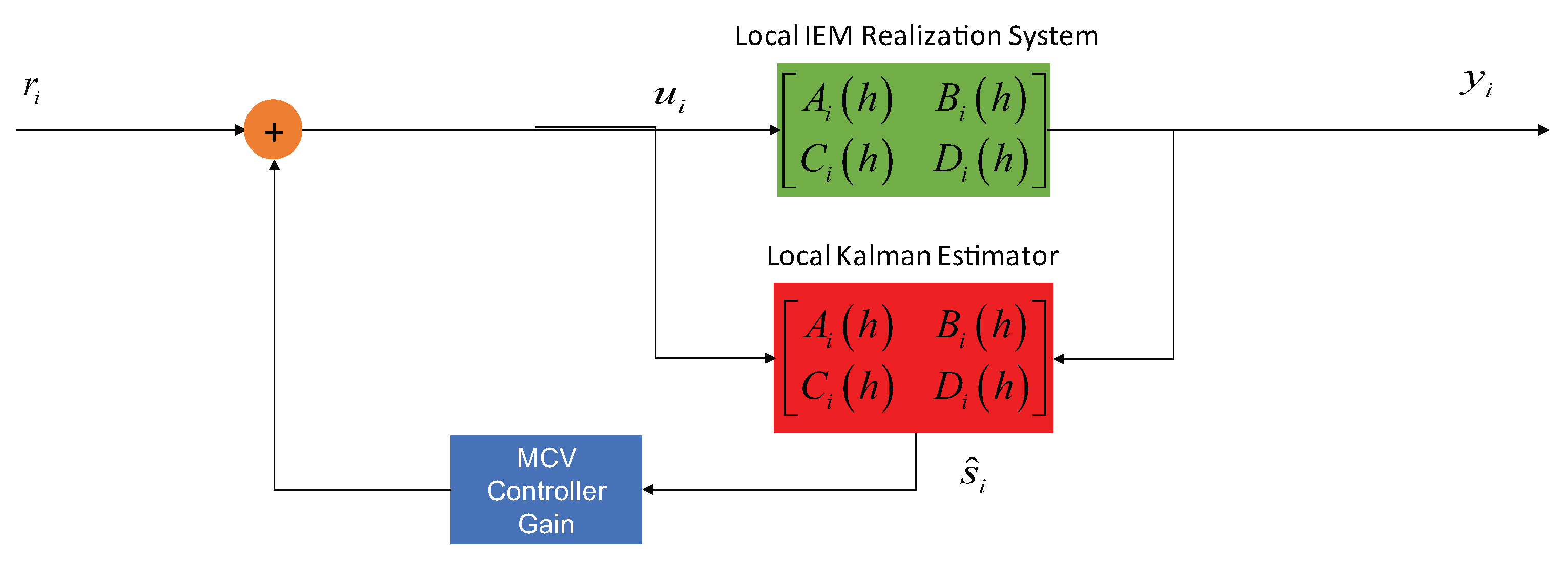
Under suitable conditions where both process and measurement noises are Gaussian, the design of stochastic control herein can be further extended and thus divided into two separate problems, one of optimal control with full state information and one of filtering. The remainder of the research investigation is to present a framework for the separation principle, which is more in line with basic engineering thinking, e.g., the optimal feedback law for steering commands is linear in the data feedback and given by
where is obtained by a local Kalman state estimator. Each platform i in Figure 11 uses the steering command (92) based on the Kalman state estimator for feedback frequency adjustments to ensure the phase offset between the steerable OCXO and the IEM estimate driven to zero.
7. Conclusions
The article has introduced the reader to an emergent timescale concept in AltPNT and some technical challenges in the new area of onboard ensemble timescale autonomy based primarily on inter-platform measurements. Admittedly, the preliminary findings herein have been an overly simplified presentation. Hopefully, they have generated heightened interest in the generation and realization of onboard ensemble timescales across pLEO constellations.
In particular, AltPNT is the key to enabling proliferated constellations intended to be reconstituted on a 3-5-year basis. It was shown that ensembling across pLEO constellations can be achieved by on-orbit assembly of flexible ensemble timescales, using the autonomous networked control of timescale realizations during and after the placement of critical information about the IEM estimation on inter-platform communication networks. The use of existing satellite crosslinks and tradeoffs between open-loop and closed-loop control manifests in the control interval and thus, becomes a dominant parameter of clock steering.
Moreover, it should be emphasized that a deep understanding of how to achieve high-precision time synchronization, resolving first-order Doppler effects on the frequency changes about received signals as a function of relative position and velocity between platforms, was investigated and is quite distinct from the existing literature on clock ensemble generation and realization. Resilient dissemination of precision timing from a distributed architecture was proposed with discreet communications between the anchor platform and separate platforms. The discreetness of IEM dissemination and data transport performance is not affected due to optimal power allocation between timing and data transports.
The autonomous assembly of active MCV controllers is the central element of steering one frequency standard very tightly to another, thus creating an onboard low SWaP timescale backup in phase and on frequency with the IEM reference. The robustness of the MCV algorithm allows reliable timescale realizations of the method even though the constituent noise processes are stochastic and performance measures are uncertain beyond the expected value.
Needless to say, the findings herein show promise in enabling some core capability concepts to achieve operational effectiveness and efficiency for ad-hoc and non-dedicated pLEOT over crosslink satellite communications under extreme radio conditions of GNSS outages, leveraging local autonomous agents running onboard pLEO constellations. These local agents provide the deep integration of communication and PNT services at the physical layer, by regulator policies derived from incumbent data link layers for link capacity resource forecasts.
Acknowledgments
The work was supported by the Air Force Research Laboratory. The views and conclusions contained herein are those of the author and should not be interpreted as necessarily representing the official policies or endorsements, either expressed or implied, of the United State Air Force.
References
- McDowell, J.C. The Low Earth Orbit Satellite Population and Impacts of the SpaceX Starlink Constellation. The Astrophysical Journal Letter 2020, 829. [Google Scholar] [CrossRef]
- Prol, F.S.; et al. Position, Navigation, and Timing (PNT) Through Low Earth Orbit Satellite: A Survey on Current Status, Challenges, and Opportunities. IEEE Access 2022, 10, 83971–84200. [Google Scholar] [CrossRef]
- Reid, T.G.; et al. Broadcast LEO Constellation for Navigation. NAVIGATION 2018, 65(2), 205–220. [Google Scholar] [CrossRef]
- Coleman, M.J.; Beard, R.L. Autonomous Clock Ensemble Algorithm for GNSS Applications. NAVIGATION: Journal of the Institute of Navigation 2020, 67. [Google Scholar] [CrossRef]
- Senior, K.L.; Coleman, M.J. The Next Generation GPS Time. NAVIGATION 2017, 64, 411–426. [Google Scholar] [CrossRef]
- Wang, Q.; Rochat, P. ONCLE (One Clock Ensemble) for Galileoś Next-Generation Robust Timing System. NAVIGATION: Journal of the Institute of Navigation 2022, 69. [Google Scholar] [CrossRef]
- Chaudhry, A.U.; Yanikomeroglu, H. Laser Intersatellite Links in a Starlink Constellation: A Classification and Analysis. IEEE Vehicular Technology Magazine 2021, 16, 48–56. [Google Scholar] [CrossRef]
- Heine, F.; et al. Status on Laser Communication Activities at Tesat-Spacecom. Free-Space Laser Communications XXXV 2023, 12413, 83–93. [Google Scholar]
- Tournear, D. Future Directions: Delivering Capabilities. In Proceedings of the Small Satellite Conference, SSC20-IV-02, 2020.
- Greenhall, C.A. Kalman Filter Clock Ensemble Algorithm That Admits Measurement Noise. Metrologia 2006, 43. [Google Scholar] [CrossRef]
- Senior, K.; Coleman, M.J. Generation of Ensemble Timescales for Clocks at the Naval Research Laboratory. In Proceedings of the 2014 Precise Time and Time Interval Meeting, 2014, 98–105.
- Tryon, P.V. and Jones, R.H. Estimation of Parameters in Models for Cesium Beam Atomic Clocks. Journal of Research of the National Bureau of Standards 1983, 88, 71–81. [Google Scholar] [CrossRef] [PubMed]
- Malykin, G.B. The Sagnac Effect: Correct and Incorrect Explanations. Physics-Uspekhi 2000, 43. [Google Scholar] [CrossRef]
- Shen, D.; Chen, G.; Pham, K.D.; Blasch, E. Enhanced Multi-Way Time Transfer for High-Precision Time Synchronization among UASs. In Proceedings of IEEE Military Communications Conference, 2022.
- Stein, S.R. Time Scales Demystified. In Proceedings of the 2003 IEEE International Frequency Control Symposium and PDA Exhibition Joinly with the 17th European Frequency and Time Forum, 2003, 223–227.
- Zucca, C.; Tavella, P. The Clock Model and Its Relationship with the Allan and Related Variances. IEEE Transactions on Ultrasonic, Ferroelectrics, and Frequency Control 2005, 52, 289–296. [Google Scholar] [CrossRef] [PubMed]
- Pham, K.D. Integrated Navigation and Communications: A Conformance Framework. In Proceedings of IEEE Aerospace Conference, 2023.
- Farina, M.; et al. A Control Theory Approach to Clock Steering Techniques. IEEE Transactions on Ultrasonics, Ferroelectrics, and Frequency Control 2010, 57, 2257–2270. [Google Scholar] [CrossRef]
- Montestruque, L.A.; Antsaklis, P.J. On The Model-Based Control of Networked Systems. Automatica 2003, 39, 1837–1843. [Google Scholar] [CrossRef]
- Pham, K.D. Minimal Variance Control of Clock Signals. In Proceedings of IEEE Aerospace Conference, 2016, 1–8.
Short Biography of Authors
 |
Dr. Khanh D. Pham is a supervisory principal aerospace engineer at the Air Force Research Laboratory/Space Vehicles Directorate and an adjunct research professor at University of New Mexico/Department of Electrical and Computer Engineering. He is a Fellow of the Institute of Electrical and Electronics Engineers (IEEE), the National Academy of Inventors (NAI), the Air Force Research Laboratory (AFRL), the Society of Photo-Optical and Instrumentation Engineers (SPIE), the Institution of Engineering and Technology (IET), the American Astronautical Society (AAS), the Royal Aeronautical Society (RAeS), the Royal Astronomical Society (RAS), the International Association for the Advancement of Space Safety (IAASS), and the Asia-Pacific Artificial Intelligence Association (AAIA). Moreover, he also is an Associate Fellow of the American Institute of Aeronautics and Astronautics (AIAA) and the Royal Institute of Navigation (RIN). Dr. Pham served as a Senior Editor for Intelligent Systems of the IEEE Transactions on Aerospace and Electronics Systems. His interests have focused on resilient positioning, navigation, and timing; satellite cognitive radios; distributed time synchronization; digital beamforming; statistical optimal control; dynamic game decision optimization; security of cyber-physical systems; and control and coordination of large-scale dynamical systems. Lastly, he holds 40 US patents. |
Figure 1.
A pLEO Capability Concept of PNT Over Communications.
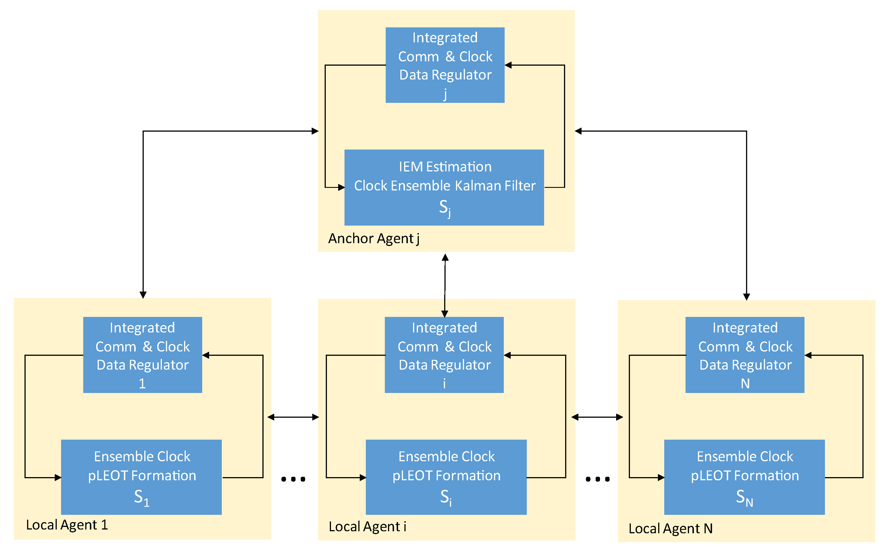
Figure 2.
Superimposing of Communication and Clock Data Signals in the Proposed ICaC.
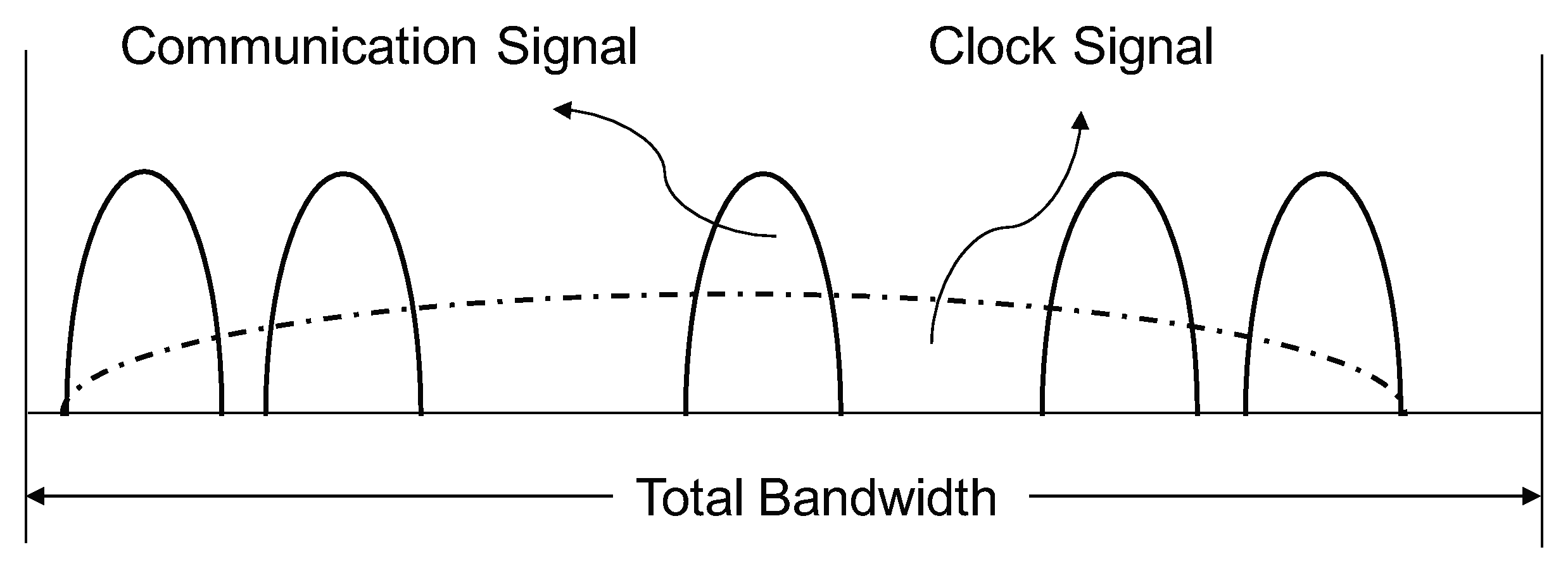
Figure 3.
A Discrete-Time System for the Proposed ICaC.
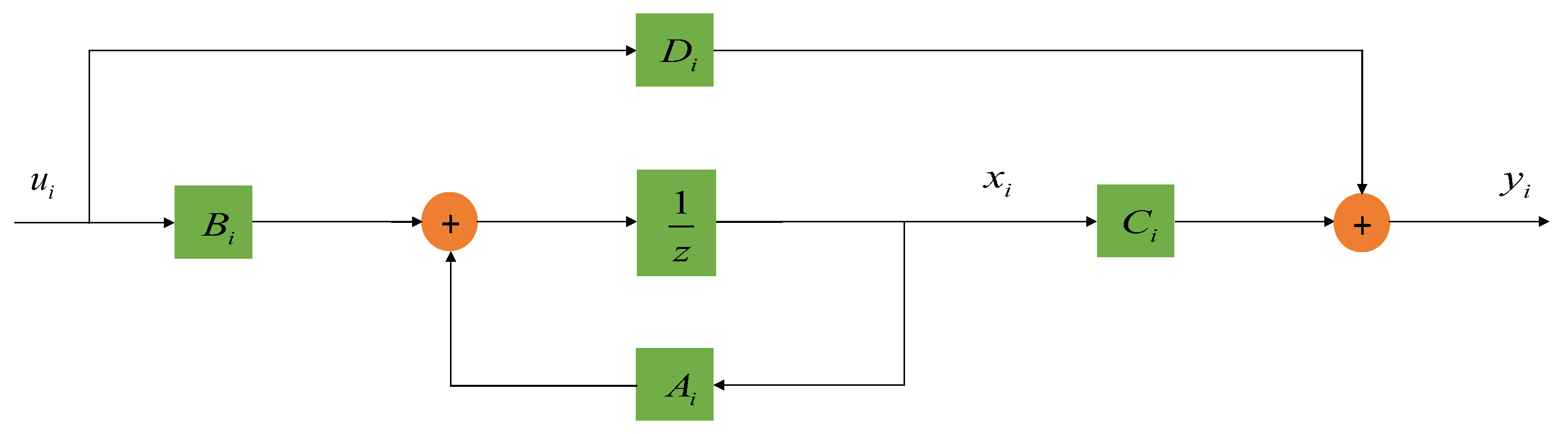
Figure 4.
Local Quadratic Regulators for the ICaC.
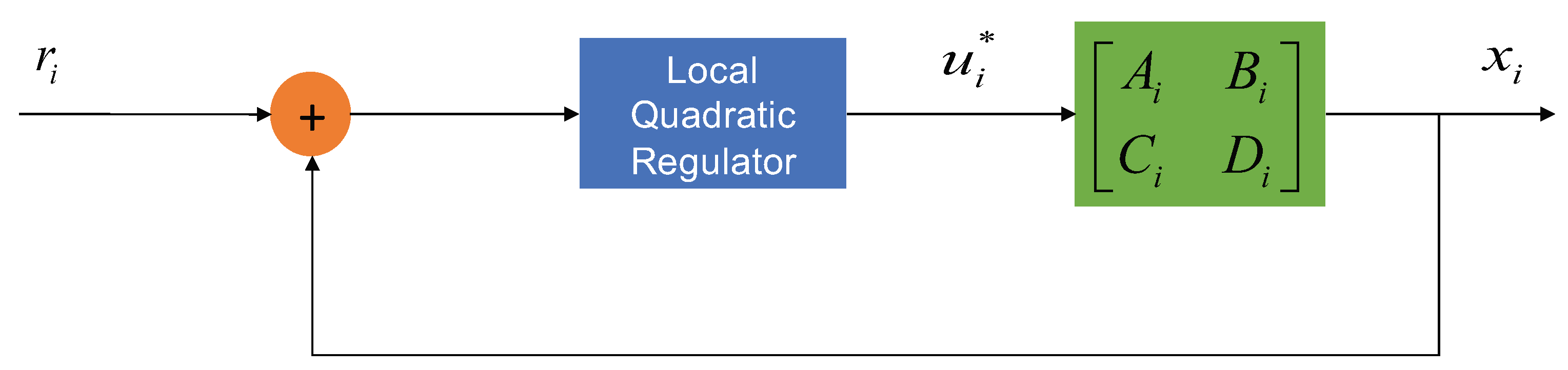
Figure 5.
A pLEOT Timescale Concept for AltPNT.
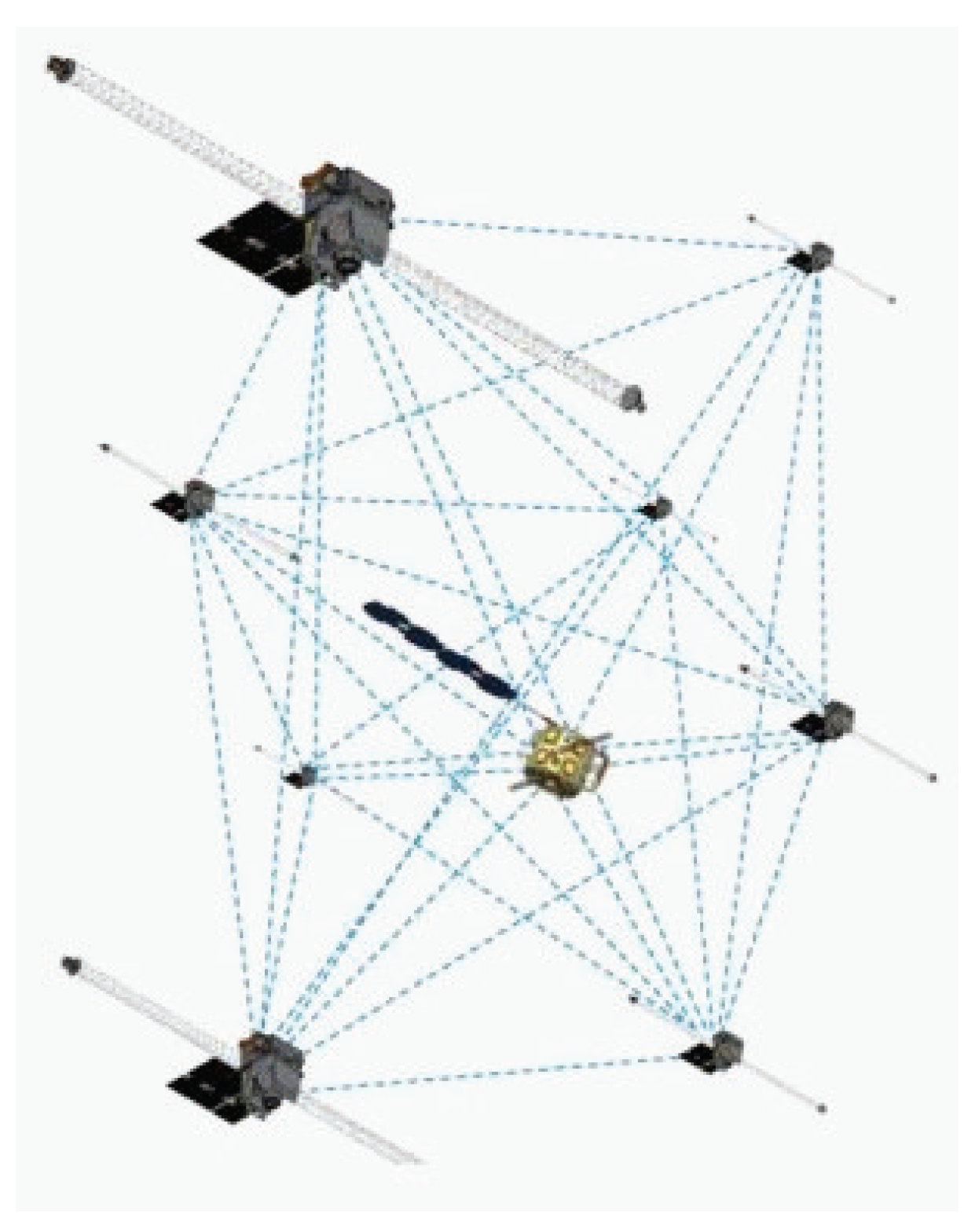
Figure 6.
Inter-Platform Measurements.
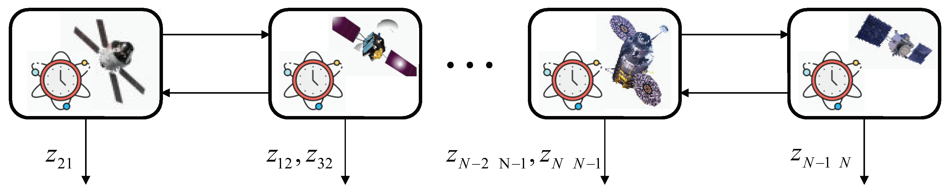
Figure 7.
The Proposed Enhanced Multi-Way Time Transfer (EM-WaTT).
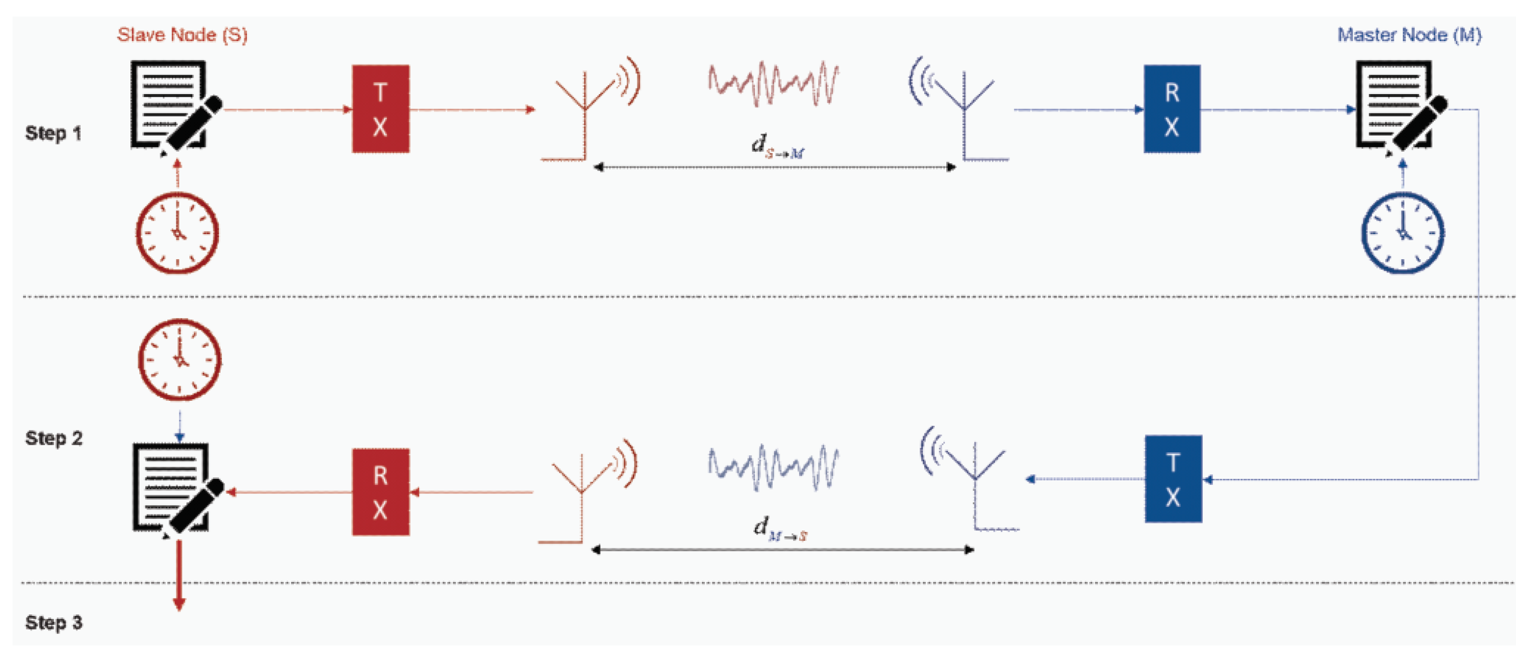
Figure 8.
Interconnections of Clock-to-Clock Difference Measurements and Kalman Filters Onboard Anchor Platform.
Figure 8.
Interconnections of Clock-to-Clock Difference Measurements and Kalman Filters Onboard Anchor Platform.
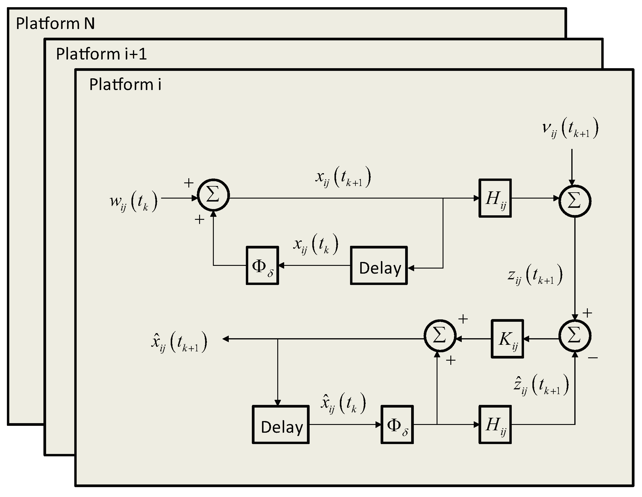
Figure 9.
IEM Realizations Aboard pLEO Platforms.
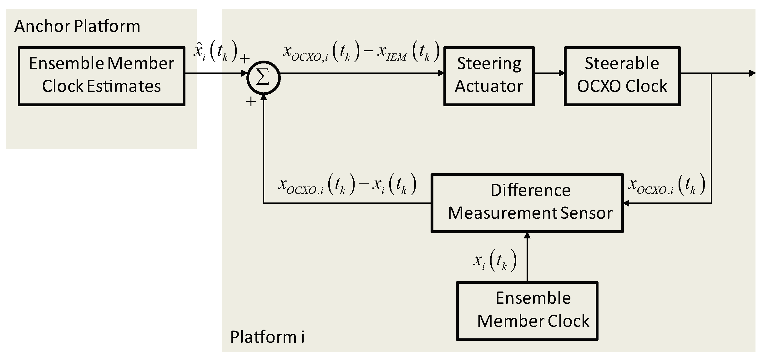
Figure 10.
Local Timescale Realizations via Networked Control Systems.
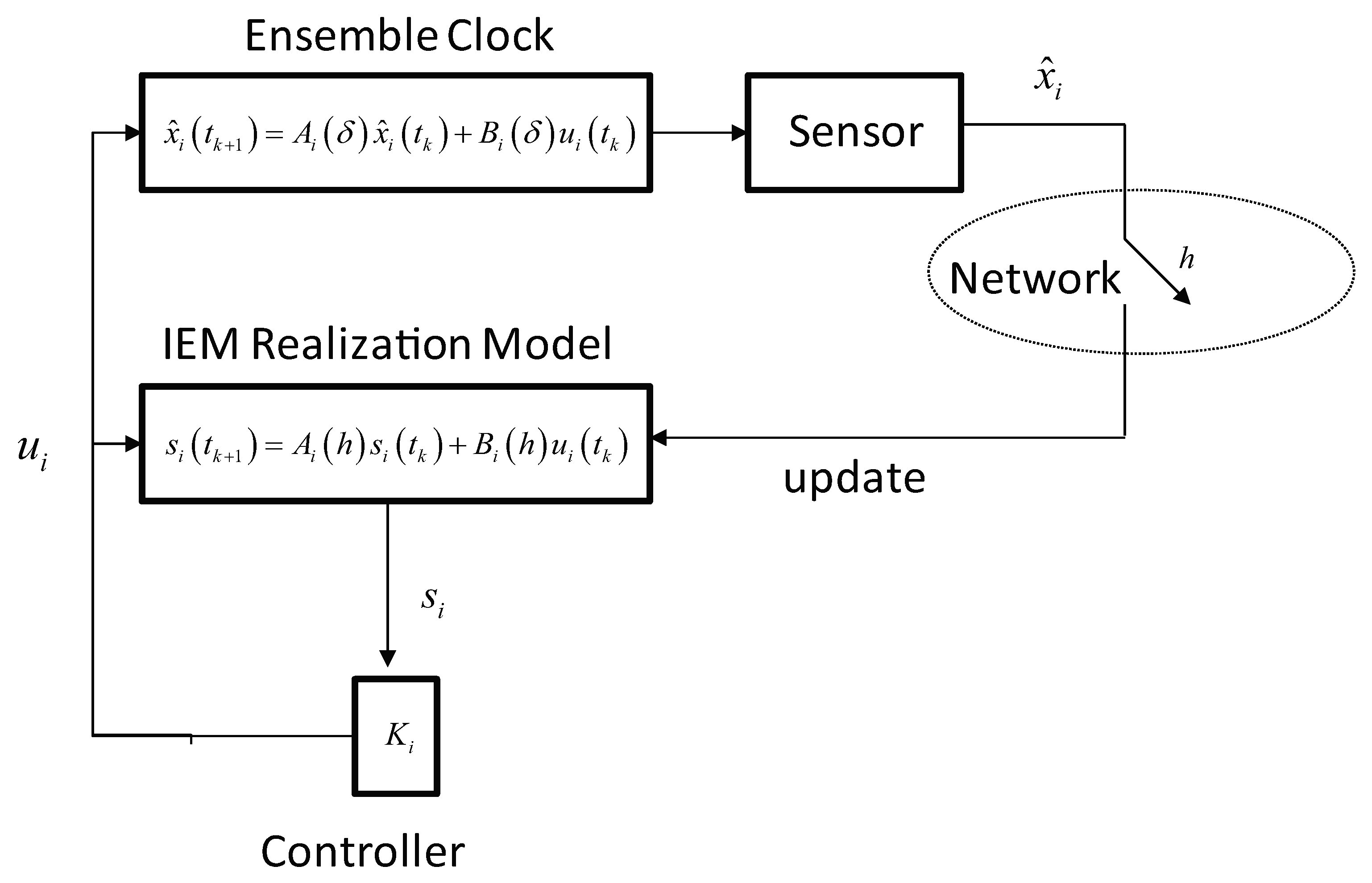
Figure 11.
Local Timescale Realizations via Kalman Estimators.
Disclaimer/Publisher’s Note: The statements, opinions and data contained in all publications are solely those of the individual author(s) and contributor(s) and not of MDPI and/or the editor(s). MDPI and/or the editor(s) disclaim responsibility for any injury to people or property resulting from any ideas, methods, instructions or products referred to in the content. |
© 2025 by the author. Licensee MDPI, Basel, Switzerland. This article is an open access article distributed under the terms and conditions of the Creative Commons Attribution (CC BY) license (http://creativecommons.org/licenses/by/4.0/).
Copyright: This open access article is published under a Creative Commons CC BY 4.0 license, which permit the free download, distribution, and reuse, provided that the author and preprint are cited in any reuse.


