Submitted:
05 December 2025
Posted:
09 December 2025
You are already at the latest version
Abstract
Traffic congestion is a complex phenomenon that displays wave-like behavior where even a clear road can be disrupted by the actions of a single driver, causing the formation of stop-and-go waves. Studying these unprecedented hurdles is necessary to understand traffic dynamics, improve AI-based traffic management systems, and enhance overall efficiency in transportation. This study analyzes data that uses real-world highway traffic at an urban city using METR-LA sensor data and NGSIM vehicle trajectories to compute stop-and-go wave propagation. Looking at each car, the speeds and distances between vehicles are analyzed with the principles of statistical mechanics, revealing regular patterns in collective traffic behavior. Speed variations in car platoons tend to grow as they spread in a non-linear fashion, just like chaotic dynamics found in other complex systems (“Butterfly effect”). The results, combining wave theory and statistical mechanics to understand and model the traffic, provide meaningful information that could help both traffic management and future physics-based studies of the same or similar complex systems.
Keywords:
Traffic flow
; stop-and-go waves
; shockwave propagation
; nonlinear dynamics
; statistical mechanics
; LWR model
; NGSIM
; METR-LA
1. Introduction
Traffic jams are an everyday phenomenon. They take up a large amount of time commuting, often hurting the efficiency of travel, yet they reveal a rich physical aspect. Waves of congestion move forward in almost like a sound wave propagating through thick moist air. Forming and dissipating without any accidents caused, they surely are an exciting thing to study unless you are late to work. Studying such a beautiful yet hated phenomenon will help us understand traffic better and contribute to the interests of autonomic vehicles or urban planning.
Imagining traffic as a system of particles makes sense. Consider each molecule/particle as a vehicle moving with the traffic. The collective movement of the traffic also seems like a flow of particles, propagating through the given medium with breaks and accelerations mostly aligning with those at their sides. From a macroscopic perspective, the sensors give us the speed, the density, and the flow of the traffic which can be compared to the waves which appear as stop and go patterns. Looking at the data from a microscopic perspective, correlation is found between typical waves and individual vehicle trajectories, where fluctuations often amplify, and interactions drive emergent jams.
The go and stop mechanism observed in such places of traffic already show much resemblance to waves. Early models like Lighthill Whitham Richards (LWR) theory treat traffic as a compressible fluid, predicting the backward travelling shockwaves that are observed in intervals of stop and go congestion. Zooming into a microscopic point of view, the traffic shows resemblance to a statistical orchestra. Though individual cars differ in speed and spacing, probability distributions come up which echo the principles of statistical mechanics. Whenever there is a slight disturbance within traffic, they can grow into large jams without any external trigger.
Most of the present studies focus either on macroscopic wave analysis or microscopic particle analysis; there are very few which focus on presenting both views in a data driven way. This study combines wave measurements from sensor data, Particle distributions from trajectories and nonlinear amplification analysis. The study starts with the assumption that traffic waves are predictable, quantifiable, and explainable with physics.
In summary, the main contributions are the following:
- (a)
- The primary objective of the study is to examine how physics-based models, often used to study at a smaller level, can be used to evaluate real life phenomenon like traffic.
- (b)
- This study Analyses the statistical properties of quantifiable measurements like car positions, traffic densities, speeds using concepts from statistical mechanics.
- (c)
- Theoretical models like Lighthill Whitham Richards (LWR) and car following models are compared to real life data.
2. Methodology
2.1. Workflow
- 1)
- Data Acquisition
This Project’s data is sourced from NGSIM, METR-LA and PeMS. The information about microscopic trajectories of each vehicle is taken from NGSIM whereas the macroscopic sensor data is taken from METR-LA and PeMS.
- 2)
- Data Preprocessing
This step is essential to refine the data we obtained from the sources. Preprocessing ensures removal of inaccurate entries. Units are standardized, time stamps are aligned for accurate computing, data is resampled into groups of consistent intervals, and everything is then checked for consistency.
- 3)
- Exploratory data analysis
This step produces the basic data necessary for the calculations later. The fundamental quantities like density, speed, and slow are obtained/ calculated in this step. Generation of visual distributions (histograms, heatmaps, etc) is followed by a brief check for anomalies and correlations.
- 4)
- Feature Engineering
Final Variable quantities like local speed variance and headway gradients are calculated from the microscopic quantities obtained from earlier steps. The macroscopic quantities are used to calculate bulk variables like shockwave speed and wave amplitude. In short, this step involves the transition of individual variables into features which capture both particle-like and wavelike aspects of traffic.
- 5)
- Predictive Modeling
Comprising of application of the engineered outputs, this step involves the building of models to predict variables based on the principles of physics like LWR or shockwave propagation.
- 6)
- Evaluation and Validation
This final step provides the concluding statement. The predicted outputs from the models made are compared to the real-life variables. The match percentage would prove/disprove our hypothesis.
2.2. Data Sources
For this data analysis, multiple datasets are essential for meaningful information to be derived from it. Specifically, this dataset approach enables us to compute traffic at both particles (using NGSIM) and macroscopic (using METR-LA and PeMS) levels.
The NGSIM dataset deals with the Microscopic Analysis and particle-level modeling of vehicles. This trajectory-based dataset is collected by the U.S. Federal Highway Administration to study traffic flow, driver behavior, and microscopic interactions. It captures vehicle trajectories at high resolution and at an Impressive Sampling rate of 10Hz. Importantly, it captures stop-and-go behavior at a car level, granted a short observation of time, usually around 15-45 minutes. The dataset covers selected highway segments, such as US-101 in Los Angeles and I-80 in the San Francisco Bay Area.
The METR-LA Dataset provides macroscopic sensor data from detectors in Los Angeles Freeway. Its main purpose comes down to complementing NGSIM by providing measurements of mainly traffic flow and speed which helps in macroscopic analysis of wave propagation.
PeMS dataset is quite like METR-LA, providing Large-scale macroscopic dataset which collects data from freeways across the entire state of California. It is a wide area with a large-scale network of sensors. This paper uses PeMS data on top of METR-LA for a broad temporal and spatial traffic analysis.
These datasets were specifically chosen to best represent the traffic globally, as contrast to datasets taken from elsewhere, which may overestimate or underestimate the stop-and-go wave propagation and may lack the resolution required for such level of physics-based modeling. The reliability of the datasets lies in their standardized data, which is provided in a clean format, eligible for robust statistical and physical analysis.
2.3. Data Preprocessing METR-LA
The raw dataset from the METR-LA dataset was converted from a HDF5 file to a structure of pandas Data frame format (in Python) with datetime indexing and sensor ID mapping. The file contains speed measurement data from 207 loop detectors on Los Angeles highways at a 5- minute interval from March to June 2012. From this data, physically impossible speeds (v < 0 or v > 100 mph) were removed, gaps ≤30 minutes were filled using linear interpolation, and sensors with >20% missing data were excluded.
Gaussian smoothing (σ = 1.5-time steps) was applied using the kernel G(t) = to reduce sensor noise while preserving traffic wave characteristics essential for the overall analysis.
PEMS
The PEMS dataset was important to determine traffic flow, speed, and occupancy measurements from California's freeway loop detectors which clocked information at a 5-minute interval. Raw data was readily available in a readable format, and the data was easily available in a readable format of required information (Speed and Occupancy being our major requirement). Invalid measurements (flow <0 or >4,000 veh/h, speeds >120 mph) were removed, gaps ≤25 minutes were filled using linear interpolation, and sensors with coordinate deficiencies were excluded.
Traffic flow data underwent smoothing using a similar technique mentioned earlier to reduce sensor noise while preserving the macroscopic wave characteristics necessary for further analysis and macroscopic observation.
NGSIM
NGSIM trajectory files were obtained from the Federal Highway Administration's repository, which was available on demand.Raw data recorded at 10 Hz was sampled to 5 Hz for optimization purposes. Vehicle trajectories require cleaning for tracking artifacts, with polynomial regression correcting physically impossible movements exceeding 15 mph speed changes between consecutive time steps.
2.4. Exploratory Data Analysis
This step plays a crucial role in splitting the path into analysis of macroscopic and microscopic levels. The data extracted after preprocessing is analyzed at both levels. While microscopic analysis is done with respect to vehicular behavior, macroscopic analysis is done with bulk behavior in mind. This step involves looking for features and patterns in the data we obtained before calculating any new instruments of measure.
Microscopic Analysis
Macroscopic analysis lays focus on individual quantities like speed, acceleration, and headway. These quantifiable numbers help us visualize and compare the individual cars of traffic with the particle sin a system of particles. The data analysis also includes mapping out histograms and other distributions of individual statistics. The distributions help us to understand how spread out or how clustered the behaviors are. The same goes for other statistics like variance which tell us the average deviation of the quantities from the central measures.
Macroscopic Analysis
Macroscopic analysis is just like the zoomed-out version of microscopic analysis. Here, instead of dealing with individual values, we deal with aggregate values like average speed, density, flow, etc. They come by averages of individual data and sensor data. This includes drawing plots of flow vs density for different types of traffic (free, congested, jammed, etc.). We can visualize the series/waves of congestions moving along the lengths of a highway and calculate the wave properties like amplitudes of the stop and go oscillations or the shockwave speeds.
2.5. Feature Engineering
The goal of feature engineering is to create or modify the data into new variables so that the system built would understand the data better. The raw measurements, both macroscopic and microscopic, are used to produce better variables for the models. Production of new variables is followed by aggregation of microscopic metrics into macroscopic ones. We establish a relation between particle level fluctuations and bulk metrics of the traffic.
Microscopic Features
The input variables include:
- Speed of the vehicle: vi
- Number of Vehicles observed in a specific segment (N)
- Average vehicular speed (vm)
- Time stamps for each vehicle’s trajectory
The features produced are:
- Local Speed Variance
Measures the average deviation for speeds in a particular time frame
Formula:
2.6. Macroscopic Features
The input variables include
- Flow count per interval (Vehicles per interval)
- Average speed reported by the sensors (vm)
- Segment length (L)
- Time interval (Δst ) The features produced are:
- 2.
- Traffic flow (q)
Represents the number of vehicles passing a point per hour.
Formula: q = × 3600
- 3.
- Density ( k )
Represents the number of vehicles per kilometer of roadways.
Formula: k = or k =
- 4.
- Shockwave speed ( ω )
Determines how fast a congestion wave travels along the highway.
Formula: ω =
- 5.
- Travel time ( T )
Estimated time to traverse the segment.
Formula: T =
2.7. Predictive Modeling
Predictive modeling includes substitution of engineered features (density, flow, and velocity) into the set models for generating predicted output variables which are used in the next step by comparing the outputs with figures from the real time data. The outputs include predicted magnitudes of traffic density, traffic speed, traffic flow, and travel time.
Physics based approach for predictive Modeling:
- 1)
- Lighthill Witham Richards Model:
This model treats the flow of traffic like that of a fluid and applies conservation of vehicles to it. It projects density evolution to the chosen fundamental diagram, giving a dynamic model for how traffic builds up and dissipates
Where:
k(x,t) is density defined as a function of time and
q(k) is the flow determined from the fundamental diagram.
- 2)
- Fundamental diagram (flow density relationship)
Fundamental diagram shows how the traffic flow q (number of vehicles per hour) changes with change in density of the traffic flow k (number of vehicles per kilometer). From the distribution, we can understand and assume that at very low density, Cars move at free flow speed, and the flow increases linearly with density. At medium density, flow is maximum; the flow at such a case is called capacity flow or qmax because the flow is maximum. The critical density lies here. At very high density, Cars slow down drastically, flow decreases even though density increases. At the extreme, when the road is totally jammed, density is the maximum kj (jam density).
From the diagram, we can identify:
- Free flow speed (vf) by calculating the slop of the initial rising part of the curve.
- Jam density (kj) by finding the density at which the cars are bumper to bumper, and the flow is zero.
- Capacity flow (qmax) by finding out the peak or the maxima of the curve.
- Critical density (kc) by identifying the value of density at qmax
- 3)
- Shockwave propagation
Any sudden change affecting the flow of traffic like a traffic signal turning green or a sudden accident might follow the pattern of a shockwave. If the density increases suddenly, the shockwave propagates backward/upstream. If the density decreases suddenly, the shockwave moves forward/downstream.
The formula for shockwave speed is:
w =
q1 and k2 are the flow and density before the change; q2 and k2 are the flow and density after the change.
2.8. Evaluation and Validation
Metrics such as Root Mean Square Error (RMSE), Mean Absolute Percentage Error (MAPE), and R2 are used to evaluate the accuracy of the predicted output.
3. Results
This section presents the findings at both the microscopic and macroscopic levels of traffic dynamics. The results are illustrated through outputs such as statistical distributions, wave patterns, heat-maps and several visualizations, which are used throught to provide a clearer view of the results and enhance the understanding for future studies.
3.1. Descriptive Statistics & Data Summary
(a) Dataset Scope
- Number of sensors: 47,256 detectors in total for PeMS database (calibrated freeway loop detectors)
- Time period: Most datasets were analyzed in a time gap of 1-3 weeks
- Sampling interval: Standard 5-minute aggregated intervals per detector
- Geographic scope: California state freeway system, focuses on I-405 southbound corridor in District 7 (Los Angeles County)
- Vehicle observations: Millions of vehicle passage events aggregated per detector per interval. It is important to note that these vehicles' data was not recorded on a public holiday.
- Spatial distribution: Detectors spaced approximately every 0.5 to 1 mile along freeway mainlines for wave tracking
3.2. Microscopic Traffic Dynamics
Traffic behavior at the vehicle level is characterized by the statistical distributions of key variables such as speed, acceleration, and occupancy. Vehicle speeds exhibit clustering around a typical free-flow speed but display a broad spread toward lower velocities, indicating the coexistence of smooth traffic and stop-and-go conditions. This spread reflects driver heterogeneity and highlights the early stages of traffic instability when some vehicles slow sharply while others maintain higher speeds.
Acceleration data further underscores variability, with most values near zero signifying cruising, but notable tails representing rapid braking and acceleration events under congested conditions. Such fluctuations demonstrate how individual driver responses can amplify and propagate through the traffic stream.
Headway distributions reveal that short gaps dominate in congested scenarios, while longer spacing is typical of free-flow traffic. This skew aligns with the behavior of interacting particle systems, where local fluctuations produce emergent large-scale traffic waves. These microscopic statistical patterns lay the foundation for understanding macroscopic traffic dynamics and wave
3.3. Integrated Interpretation
These findings from a microscopic and macroscopic perspective reflect traffic as a system having dualistic properties. Focusing on isolated vehicles, variations of speed, sharp accelerations, and small headways show a particle-like depiction wherein local interaction is dominant, and small disturbances are constantly fed into the flow. When considering an aggregate scale, those same disturbances appear as a group of patterns that behave like waves wherein congestion propagates backward in the stream much like shockwaves when dealing with fluids. The relationship between the two viewpoints is rooted in the enhancement of minor variations. A solitary driver applying brakes modestly can instigate a series of reactions, which propagate across numerous vehicles and ultimately culminate in a substantial traffic congestion. This responsiveness to initial circumstances is a defining characteristic of nonlinear dynamics, wherein minute randomness gives rise to significant order, manifesting as repetitive stop-and-go patterns.
While the examination reveals such emerging trends, it is important to note some of its limitations. Datasets only refer to specific freeway sections and prescribed time periods, and exogenous variables like meteorological conditions, accidents, or driver heterogeneity might have influences that are not completely captured in this work. Still, the results support the view that traffic must not only be thought of as a collection of cars or an unbroken flow, but as an intricate system where microscopic behaviors and macroscopic movements are deeply interrelated.
The PeMS and METR-LA datasets expose several recurring patterns that exemplify wave-like phenomena in real freeway traffic, with each graph revealing a distinct part of this process. The time series plot of average speed clearly displays persistent, sharp drops in speed over long periods, showing that traffic does not maintain a steady state but alternates rhythmically between fast (free flow) and slow (congested) conditions. This rhythmic shift is not isolated, but repeats as a cycle, resembling oscillations seen in physical wave systems.
The space-time heatmap of speeds adds another layer of insight. The bands of reduced speed do not simply appear and disappear at random locations but travel across the highway network, creating diagonal streaks. This movement of congestion is typical of a backward-propagating wave, where a disturbance (such as braking) affects following vehicles, causing the low-speed region to migrate upstream.
Looking at the speed distribution heatmap, sensors positioned along the corridor do not all experience the same conditions at the same time. Some locations have a clustering of speeds near the free-flow regime, while others show a wider range, with repeated transitions between high and low values. This spread is a consequence of the wave’s passage—sensors caught in the wave trough see broad, slow conditions, while those outside the wave maintain steady, high speeds.
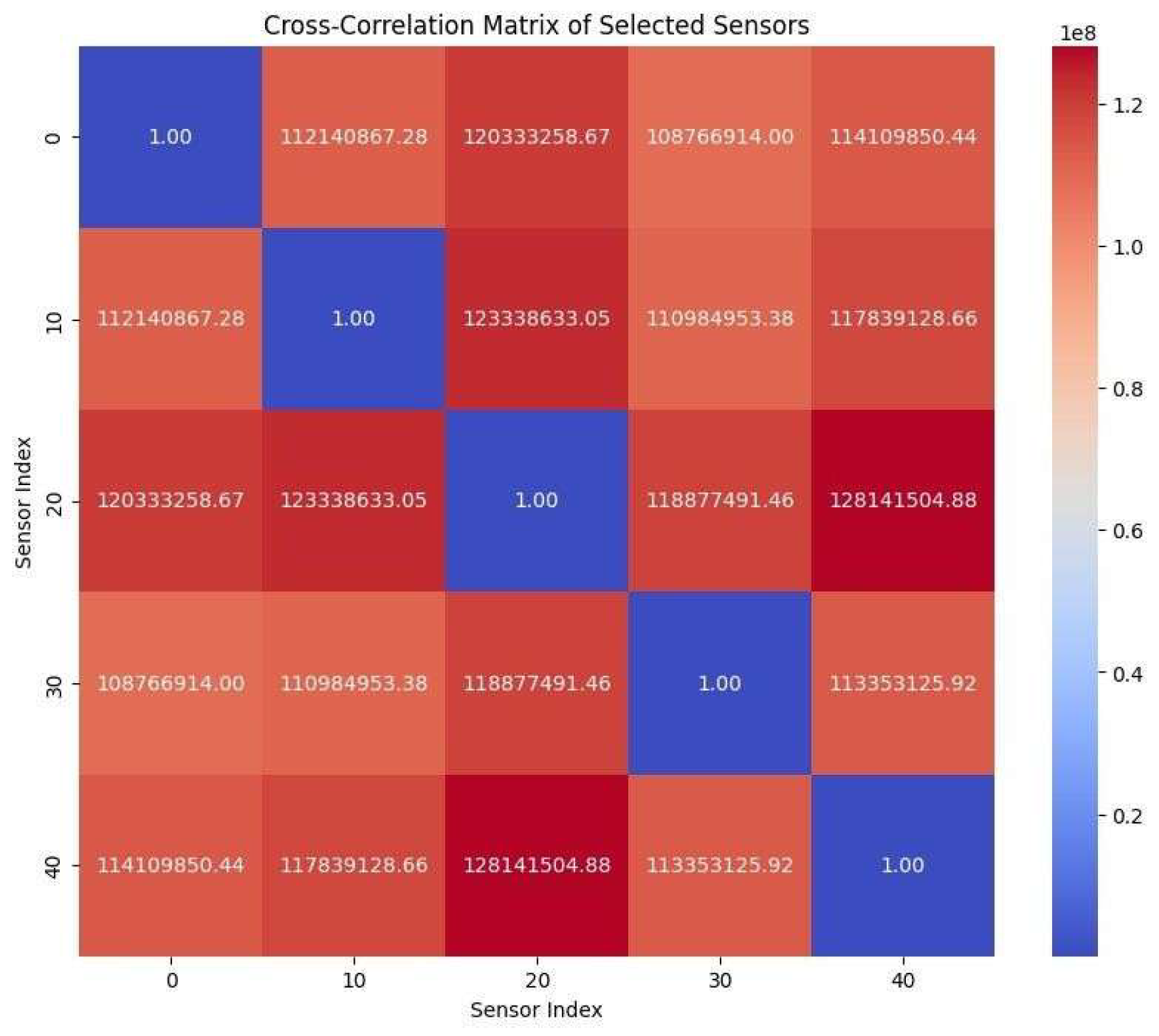
The cross-correlation matrix further illuminates the spatial coherence of these patterns. High correlation values between sensor pairs imply that changes in traffic at one point are strongly linked to changes elsewhere; these connections are robust even between sensors that are not immediately adjacent, reinforcing the idea of a traveling influence rather than random, local changes.
Taken together, the contexts drawn from these graphs illustrate how stop-and-go waves in real traffic are the result of regular, organized disruptions that migrate over space and time, producing clear and repeatable patterns in speed and flow across the network. The interplay between local events and system-wide effects is visible in both the temporal oscillations and the spatial progression of traffic states.
The relevant microscopic data plots used to deduce the information are shown below.
Figure 3.
3A Average Speed over time.
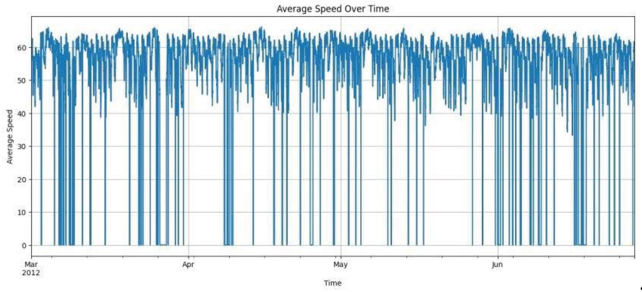
Figure 3.
3B Speed-Time Heatmap of speed.
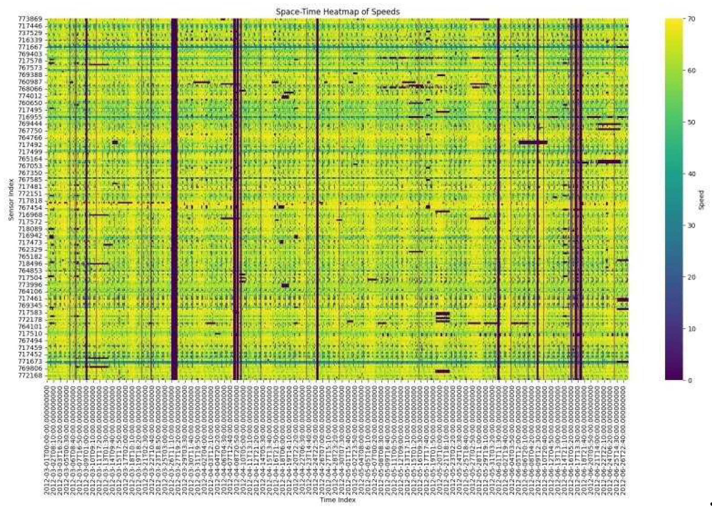
Figure 3.
3C Heatmap of Speed distribution.
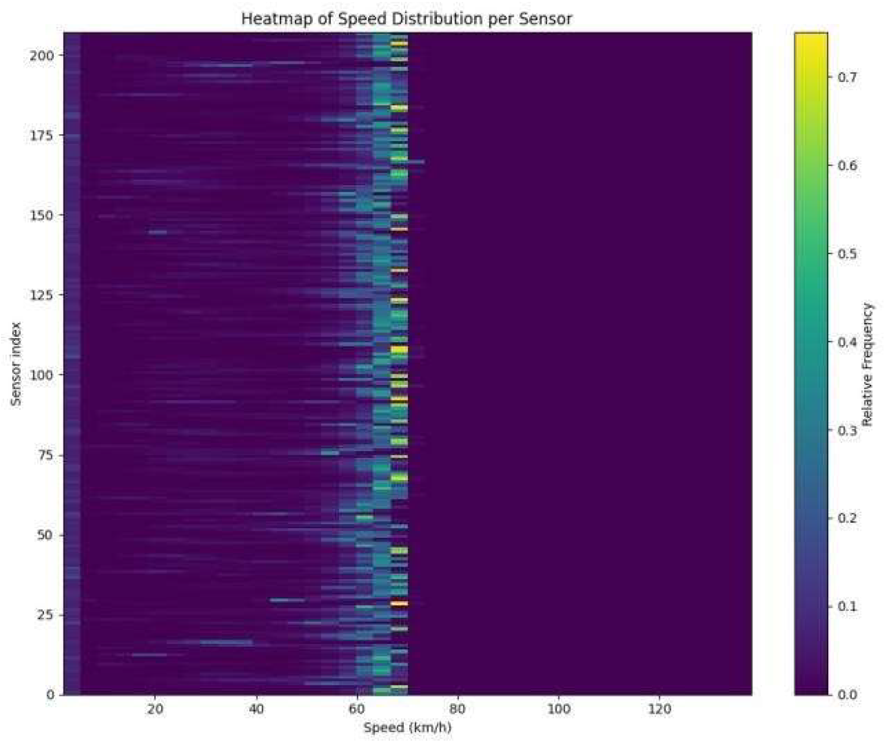
Figure 3.
3D Cross-Correlation Matrix of sensors.
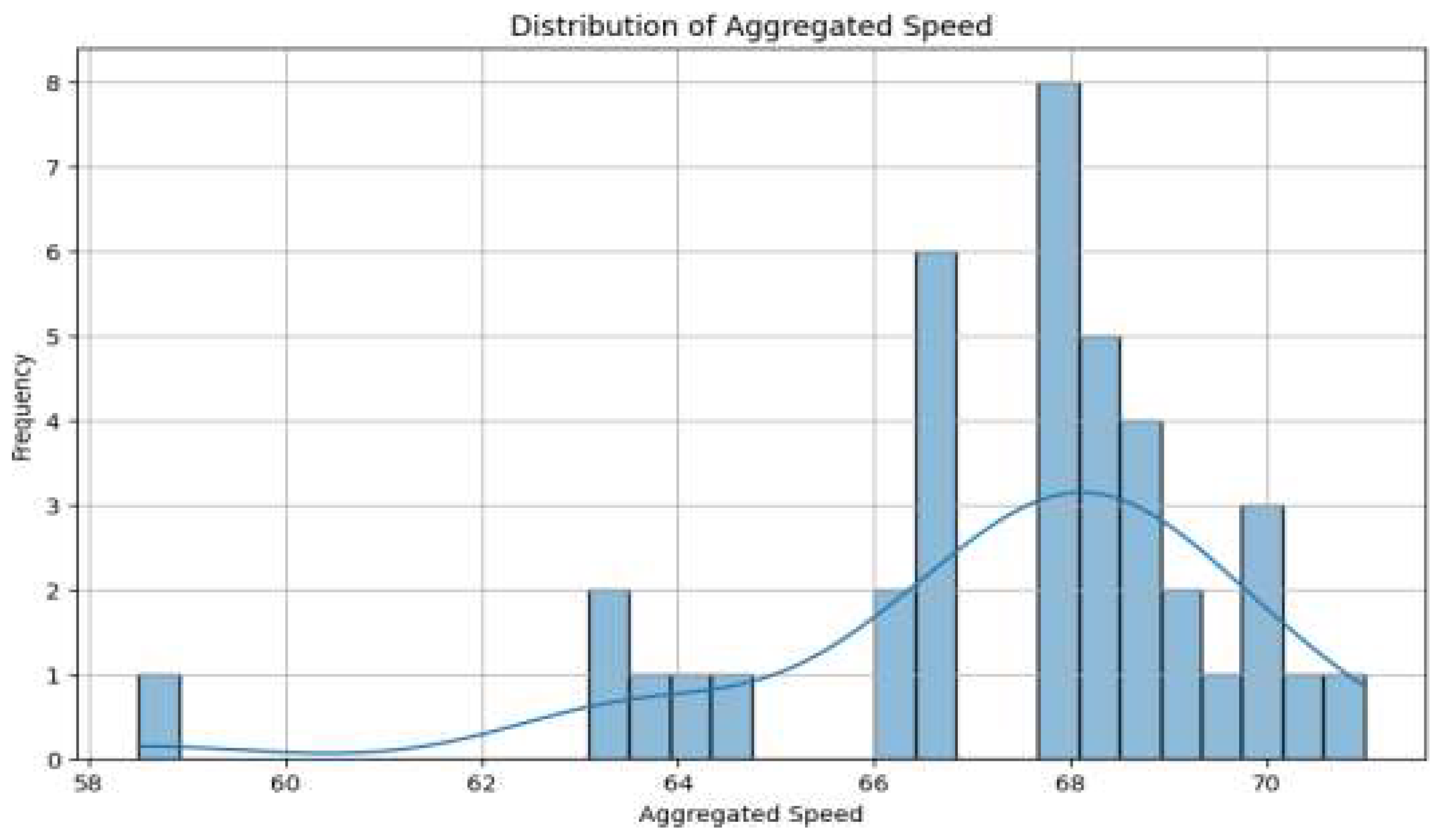
The macroscopic sensor data offers insight into the overall speed patterns across the highway network. The histogram of aggregated speed demonstrates that most sections operate within a relatively narrow band of optimal speeds, with the majority of observations clustering around the higher end of the range. This suggests that the freeway generally functions under free-flow conditions but also hints at occasional deviations likely caused by congestion or disturbances.
The accompanying dot plot, which relates aggregated speed to absolute postmile, highlights the spatial variability of traffic: some locations consistently maintain high speeds, while others show abrupt drops. Together, these visualizations capture both the typical travel behavior seen across the network and the pockets of reduced performance that can arise due to wave-like disruptions, underscoring the importance of macroscopic data in understanding traffic flow dynamics. The relevant macroscopic data plots used to deduce the information are shown below.
Figure 3.
3E Speed vs Absolute Postmile.
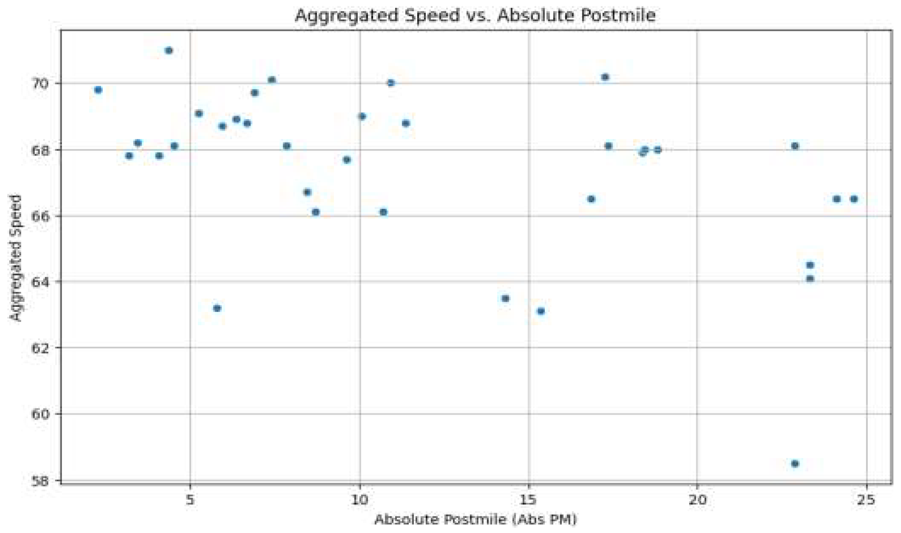
Figure 3.
3F Distribution of Aggregated.
4. Conclusion
Given the graphs, it is a valid and an interesting conclusion we can make here that understanding Traffic, stop and go waves specifically, as waves showing wave-like behavior and properties: patterns identified in the traffic data emerge through multiple forms of graphical analysis, each contributing a different perspective. Space-time heatmaps illustrate not only where congestion arises, but how it spreads across the network, making it possible to observe backward-moving waves. All in all, the analysis can lead us to a definitive conclusion that Free way traffic does indeed show wave-like properties, and it is best understood that way to study spontaneous disturbances like stop-and-go waves in future. This piece of information which is concluded can drastically Improve further studies in this specific field.
Related Works
References
- Ahn, S., Laval, J.A., & Zheng, Z. (2015). Stop-and-go waves in congested highway traffic: Empirical observations and theoretical modeling.
- Dhamge, N.R., Patil, J., Dhakate, M., & Hingnekar, H. (2023). Study of Characteristics of Traffic Flow. https://www.ijraset.com/research-paper/study-of-characteristics-of-traffic-flow.
- Federal Highway Administration. Moving Ahead: Study Conclusions. https://www.fhwa.dot.gov/reports/movingahead/study-conclusions.htm.
- Transportation Research Board. (1985). Traffic Flow Theory (Special Report 165). https://onlinepubs.trb.org/onlinepubs/sr/sr165/165.pdf.
- Kerner, B. S. (2004). The Physics of Traffic. [CrossRef]
- Treiber, M., Kesting, A., & Helbing, D. (2010). Three-phase traffic theory and two-phase models with a fundamental diagram in the light of empirical stylized facts. [CrossRef]
- Ma, X., Dong, Z., & Chen, F. (2017). Spatiotemporal analysis of urban road congestion during and after lockdown.
- Laval, J., & Leclercq, L. (2010). A mechanism to describe the formation and propagation of stop-and-go waves in congested freeway traffic. [CrossRef]
- Orosz, G., Wilson, R. E., & Krauskopf, B. (2009). Global bifurcation investigation of an optimal velocity traffic model with driver reaction time. Nagel, K., & Schreckenberg, M. (1992). A cellular automaton model for freeway traffic. [CrossRef]
Disclaimer/Publisher’s Note: The statements, opinions and data contained in all publications are solely those of the individual author(s) and contributor(s) and not of MDPI and/or the editor(s). MDPI and/or the editor(s) disclaim responsibility for any injury to people or property resulting from any ideas, methods, instructions or products referred to in the content. |
© 2025 by the authors. Licensee MDPI, Basel, Switzerland. This article is an open access article distributed under the terms and conditions of the Creative Commons Attribution (CC BY) license (http://creativecommons.org/licenses/by/4.0/).
Copyright: This open access article is published under a Creative Commons CC BY 4.0 license, which permit the free download, distribution, and reuse, provided that the author and preprint are cited in any reuse.


