Ismail’s Contemporary Pointwise Stationary Fluid Approximation Theory: Discovering the Unknown Transitions Between Stability, Traffic Intensity, and Chaos of the Non-Stationary

1. Introduction

Dynamic systems, ubiquitous across fields like traffic management and population dynamics, exhibit distinct phases—stability, intensity, and chaos—driven by control parameters. While prior work extensively explored positive domains of $k$ and $\rho$, the behavior of negative $k$ remains largely uncharted. This study explores negative k as parallels to phenomena like negative quantum states. Building on (Mageed, 2024a) (Mageed, 2024b) (Mageed & Zhang, 2023) (Mageed, 2024d) (Mageed, 2024e) and recent advancements in perplexity AI (Mageed, 2024c), we delve into the stability, traffic intensity, and chaotic responses of systems defined by:

$$\sigma ={\left({\displaystyle \frac{k\rho +\sigma -1}{k\rho }}\right)}^k$$

(1)

By varying the values of $k(-100\le k<0)$ and ρ, we aim to reveal how these parameters influence system dynamics and transitions.

Let $f_{in}\left(t\right)$ and $f_{out}\left(t\right)$ serve as the temporal flow in (1-5), and flow out, respectively. Therefore, by Equation (2)

$${{\displaystyle \frac{dx\left(t\right)}{dt}}=x}^{.}\left(t\right)=-f_{out}\left(t\right)+f_{in}\left(t\right),x\left(t\right)\mathrm{a}\mathrm{s} \mathrm{t}\mathrm{h}\mathrm{e} \mathrm{s}\mathrm{t}\mathrm{a}\mathrm{t}\mathrm{e} \mathrm{v}\mathrm{a}\mathrm{r}\mathrm{i}\mathrm{a}\mathrm{b}\mathrm{l}\mathrm{e}$$

(2)

$f_{out}\left(t\right)$ links server utilization, $\rho \left(t\right),$ and the time-dependent mean service rate, $\mu \left(t\right)$ by (3):

$$f_{out}\left(t\right)=\mu \left(t\right)\rho \left(t\right)$$

(3)

For an infinite queue waiting space, defined by Equation (4):

$$f_{in}\left(t\right)=\mathrm{M}\mathrm{e}\mathrm{a}\mathrm{n} \mathrm{a}\mathrm{r}\mathrm{r}\mathrm{i}\mathrm{v}\mathrm{a}\mathrm{l} \mathrm{r}\mathrm{a}\mathrm{t}\mathrm{e}=\lambda \left(t\right)$$

(4)

Thus (2) rewrites to Equation (5):

$$x^{.}\left(t\right)=-\mu \left(t\right)\rho \left(t\right)+\lambda \left(t\right),1>\rho \left(t\right)={\displaystyle \frac{\lambda \left(t\right)}{\mu \left(t\right)}}>0$$

(5)

With

$$\rho \left(t\right)=\left(1-\sigma \left(t\right)\right)x\left(t\right)$$

(6)

The $GI/M/1$ PSSFA for the non-stationary $E_k/M/1$ queue reads as:

$$x^{.}\left(t\right)=-\mu \left(t\right)\rho \left(t\right)=\left(1-\sigma \left(t\right)\right)x\left(t\right)+\lambda \left(t\right),\sigma ={\left({\displaystyle \frac{k\rho }{k\rho +\left(1-\sigma \right)}}\right)}^k$$

(7)

Where $k$defines positive number of set of phases, i.e., $k=\mathrm{1,2},\mathrm{3,4},\dots$

Problem Definition

This study focuses on addressing the following phases:

• Stability Phase: Explore how σ changes for ρ ∈ [0.1, 0.999] and k ∈ [−100, 1].
• Traffic Intensity Phase: Examine system behaviour when ρ = 1 and k ∈ [−100, 1].
• Chaotic Phase: Investigate the system response for ρ > 1 (e.g., 2, 3, 4) and k ∈ [-100, −1].

In other words, we are looking at Equation (7) from a different end of the spectrum, by choosing $k=-1,-2,-3,-4,\dots$

The current breakthrough utilizes computational tools to visualize these relationships, ensuring an accurate representation of transitions between these phases for the unexplored phenomenal negative values of the numbers of sets of phases, namely, $k.$ In mathematical terms, the current exposition marks a new phenomenal chapter of rethinking the totality of PSFFA theory to shift the longstanding unresearched topic of PSFFA into a higher level of thinking between such unparallel scientific disciplines, within the chaos, quantum mechanics, random walks, Brownian motion and much more. Having seen the results of this research, it is anticipated that further investigations into more unexplored cases will expand on Ismail’s Contemporary PSFFA Theory and merge it with numerous multi-interdisciplinary spectrums of human knowledge.

2. Methodology

The methodology employs a computational framework implemented in Python to approximate σ iteratively and analyze its behavior under varying conditions. Below are the key steps:

• Equation: The sigma (σ) function is computed iteratively for combinations of $k$ and $\rho$:

  $${\sigma }_{\left(new\right)}={\left({\displaystyle \frac{k\rho +\sigma -1}{k\rho }}\right)}^k$$

  (8)

  with σ_(initial) =0.5, updated until σ_(new)− σ_(old)< 10⁻⁶ or a maximum of 100 iterations. It is to be noted that, having transformed Equation (7), into the phenomenally defined, of Equation (8), then
• Algorithm:
  • Error handling ensures robustness against division by zero, returning NaN for undefined cases.
  • Three distinct phases are explored:

    °

    Stability Phase: $0.1\le \rho <1$ and $k\in [1,100].$

    °

    Traffic Intensity Phase: $\rho =1$ with varying $k$.

    °

    Chaotic Phase: $\rho >1$ and $k\in [1,100].$

• Visualization:
  • 2D and 3D plots illustrate the relationships between $\sigma ,k$, and $\rho$.
  • Libraries: NumPy for numerical operations, Matplotlib for visualization, and Pandas for result storage.

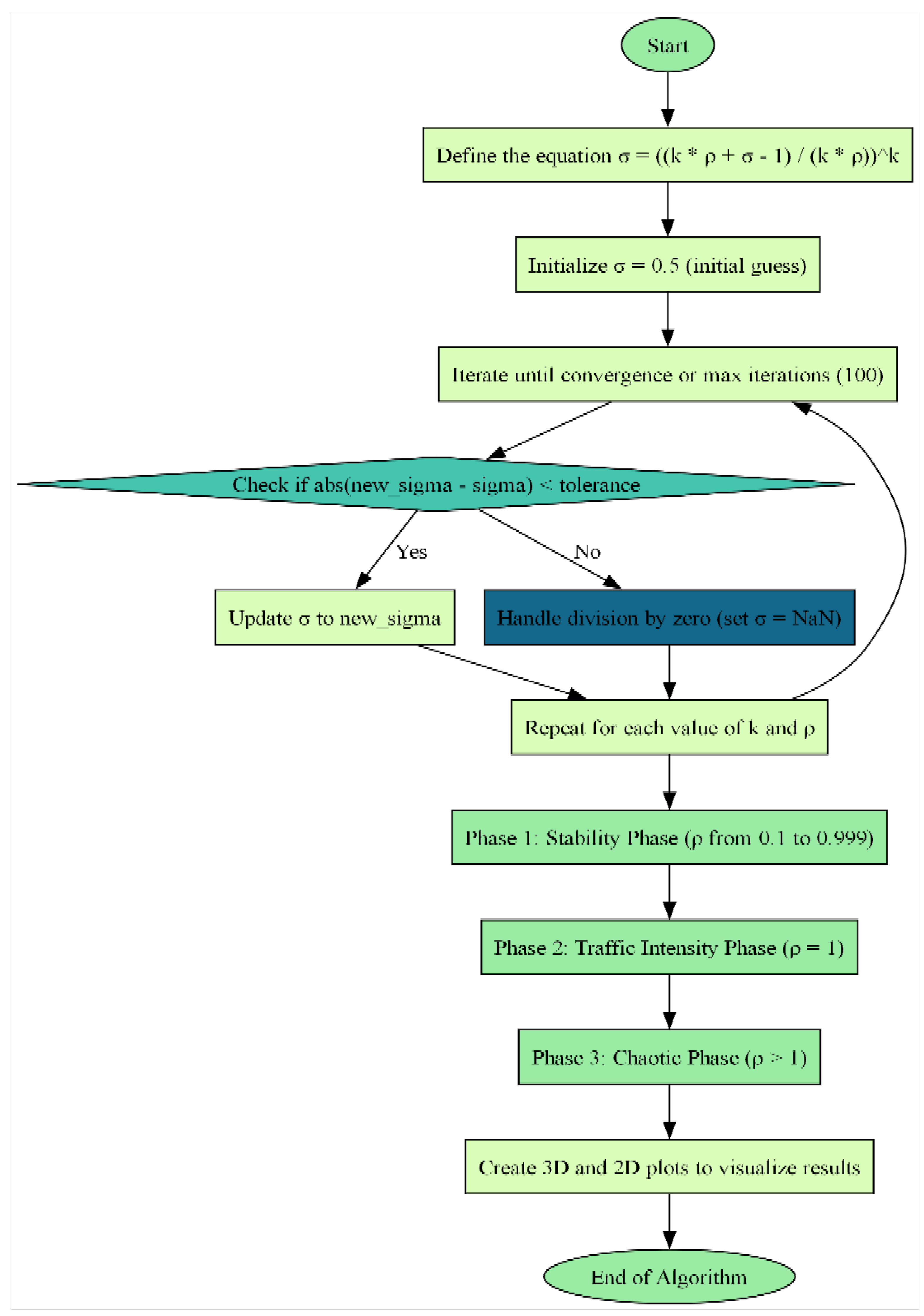
In what follows, the Pseudocode Diagram is visualized.

Figure 1. Pseudocode Diagram.

Figure 1. Pseudocode Diagram.

Here is the source code of the program:

import numpy as np

import matplotlib.pyplot as plt

from mpl_toolkits.mplot3d import Axes3D

from scipy.optimize import fsolve

import os

# Function to compute sigma numerically

def sigma_equation(sigma, k, rho):

return ((k * rho + sigma - 1) / (k * rho))**k - sigma

def compute_sigma(k, rho):

if k == 1:

return 1.0

initial_guess = 0.5 if rho < 1 else 1.5

sol, = fsolve(sigma_equation, initial_guess, args=(k, rho))

return sol

# Prepare output directory

os.makedirs(“3d_phase_plots”, exist_ok=True)

# k values

k_values = np.arange(1, 101)

# --- Stability Phase ---

rho_stability = np.linspace(0.01, 0.99, 50)

K, RHO = np.meshgrid(k_values, rho_stability)

SIGMA = np.vectorize(compute_sigma)(K, RHO)

fig = plt.figure(figsize=(12, 8))

ax = fig.add_subplot(111, projection=‘3d’)

ax.plot_surface(K, RHO, SIGMA, cmap=‘viridis’)

ax.set_title(‘Stability Phase (ρ in (0,1))’)

ax.set_xlabel(‘k’)

ax.set_ylabel(‘ρ’)

ax.set_zlabel(‘σ’)

plt.tight_layout()

plt.savefig(“3d_phase_plots/stability_phase_3d.png”)

plt.show()

# --- Traffic Intensity Phase ---

rho_traffic = np.array([1.0])

K, RHO = np.meshgrid(k_values, rho_traffic)

SIGMA = np.vectorize(compute_sigma)(K, RHO)

fig = plt.figure(figsize=(12, 6))

ax = fig.add_subplot(111)

ax.plot(k_values, SIGMA.flatten(), color=‘red’)

ax.set_title(‘Traffic Intensity Phase (ρ = 1)’)

ax.set_xlabel(‘k’)

ax.set_ylabel(‘σ’)

plt.tight_layout()

plt.savefig(“3d_phase_plots/traffic_intensity_phase_2d.png”)

plt.show()

# --- Chaotic Phase ---

rho_chaotic = np.linspace(1.1, 3.0, 50)

K, RHO = np.meshgrid(k_values, rho_chaotic)

SIGMA = np.vectorize(compute_sigma)(K, RHO)

fig = plt.figure(figsize=(12, 8))

ax = fig.add_subplot(111, projection=‘3d’)

ax.plot_surface(K, RHO, SIGMA, cmap=‘plasma’)

ax.set_title(‘Chaotic Phase (ρ > 1)’)

ax.set_xlabel(‘k’)

ax.set_ylabel(‘ρ’)

ax.set_zlabel(‘σ’)

plt.tight_layout()

plt.savefig(“3d_phase_plots/chaotic_phase_3d.png”)

plt.show()

print(“✅ All 3D phase plots generated in ‘3d_phase_plots/’ folder and displayed.”)

The pseudocode is structured as follows:

The pseudocode provided in the flowchart serves as a visual guide to implementing the iterative computational framework for analyzing σ in dynamic systems with negative $k$. It encapsulates the step-by-step logic of the algorithm used to explore the stability, traffic intensity, and chaotic phases. Below is a detailed explanation of the key components:

• Initialization:
  • The algorithm begins by defining the equation:

    $$\sigma ={\left({\displaystyle \frac{k\rho +\sigma -1}{k\rho }}\right)}^k$$
  • The initial value of $\sigma$ is set to 0.50, which is a starting point for the iterative approximation.
• Iterative Process:
  • The algorithm repeatedly calculates a new value of σ based on the equation above.
  • Convergence is determined by checking if the absolute difference between the new σ and the previous σ falls below a specified tolerance (10⁻⁶).
• Error Handling:
  • Division by zero or undefined operations are managed by assigning NaN (Not a Number) to σ, ensuring the algorithm remains robust and does not crash.
• Phases:
  • Stability Phase:

    °

    Iterates over a range of $\rho$values from 0.1 to 0.999 and k from −100 to −1.

    °

    Generates a 3D plot to visualize σ as a function of k and ρ.

  • Traffic Intensity Phase:

    °

    Fixes $\rho =1$ and varies k, producing a 2D plot of σ versus k.

  • Chaotic Phase:

    °

    Explores $\rho >1$ with varying k, generating 3D visualizations of chaotic behaviour.

Significance: The pseudocode is instrumental in systematically exploring the behavior of σ under negative k, providing the foundation for the visualizations and insights presented in the results section. It emphasizes robustness and adaptability, accurately representing system dynamics across phases.

3. Results

Visualization

Stability Phase:

Figure 2. (Stability Phase 3D Plot): The surface plot shows a gradual increase in σ as ρ and k increase. This highlights regions of stability under varying conditions.

Figure 2. (Stability Phase 3D Plot): The surface plot shows a gradual increase in σ as ρ and k increase. This highlights regions of stability under varying conditions.

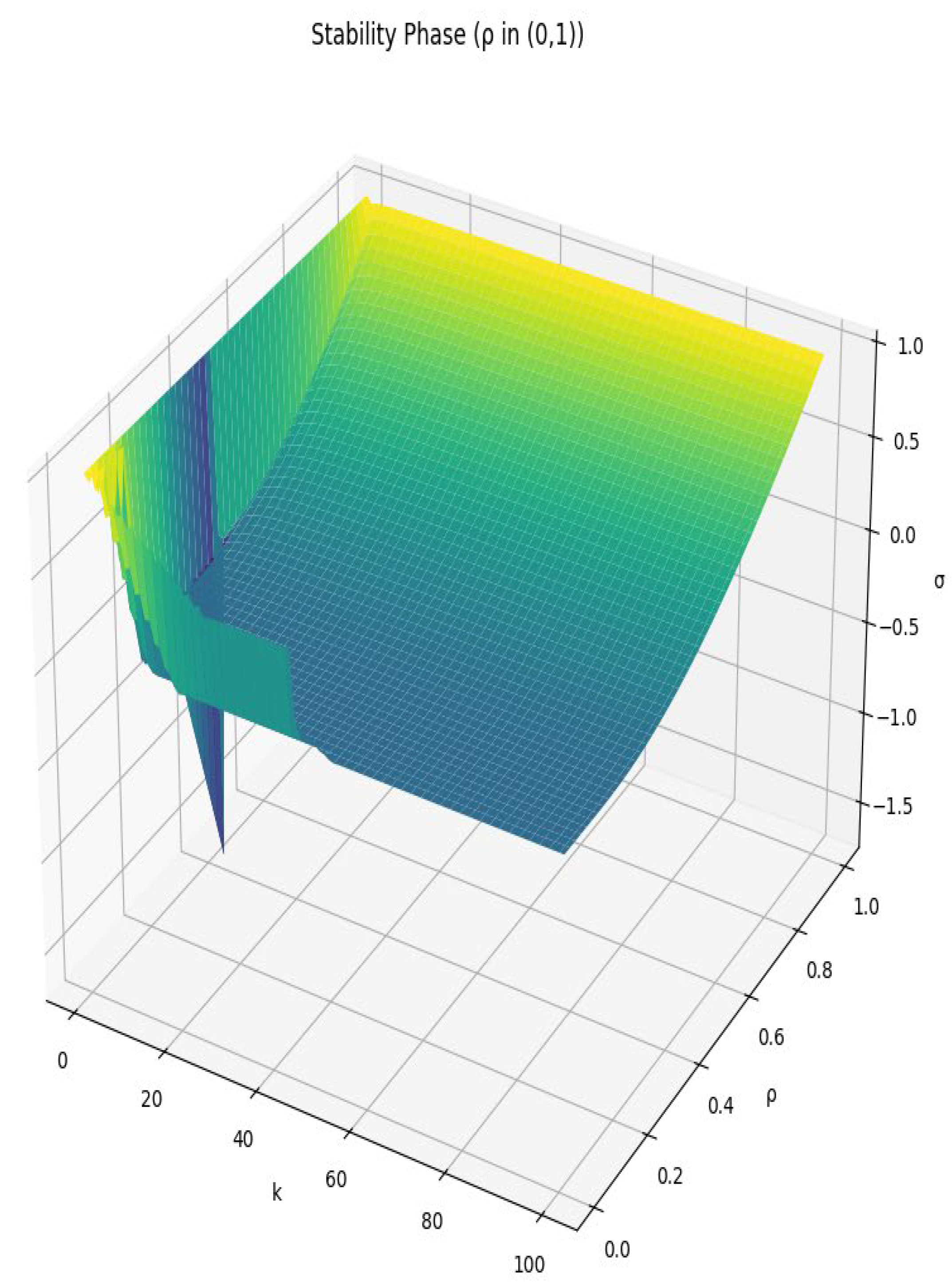
As shown by Figure 2, it is seen that for k = 1, 2…, 100, the stability phase, adhering 1> ρ > 0, the root parameter σ will follow the stability dynamics.

Traffic Intensity Phase:

Figure 3. (Traffic Intensity Phase 2D Plot): The curve demonstrates a saturation effect, where $\mathit{\sigma }$ approaches a constant value as $\mathit{k}$ increases.

Figure 3. (Traffic Intensity Phase 2D Plot): The curve demonstrates a saturation effect, where $\mathit{\sigma }$ approaches a constant value as $\mathit{k}$ increases.

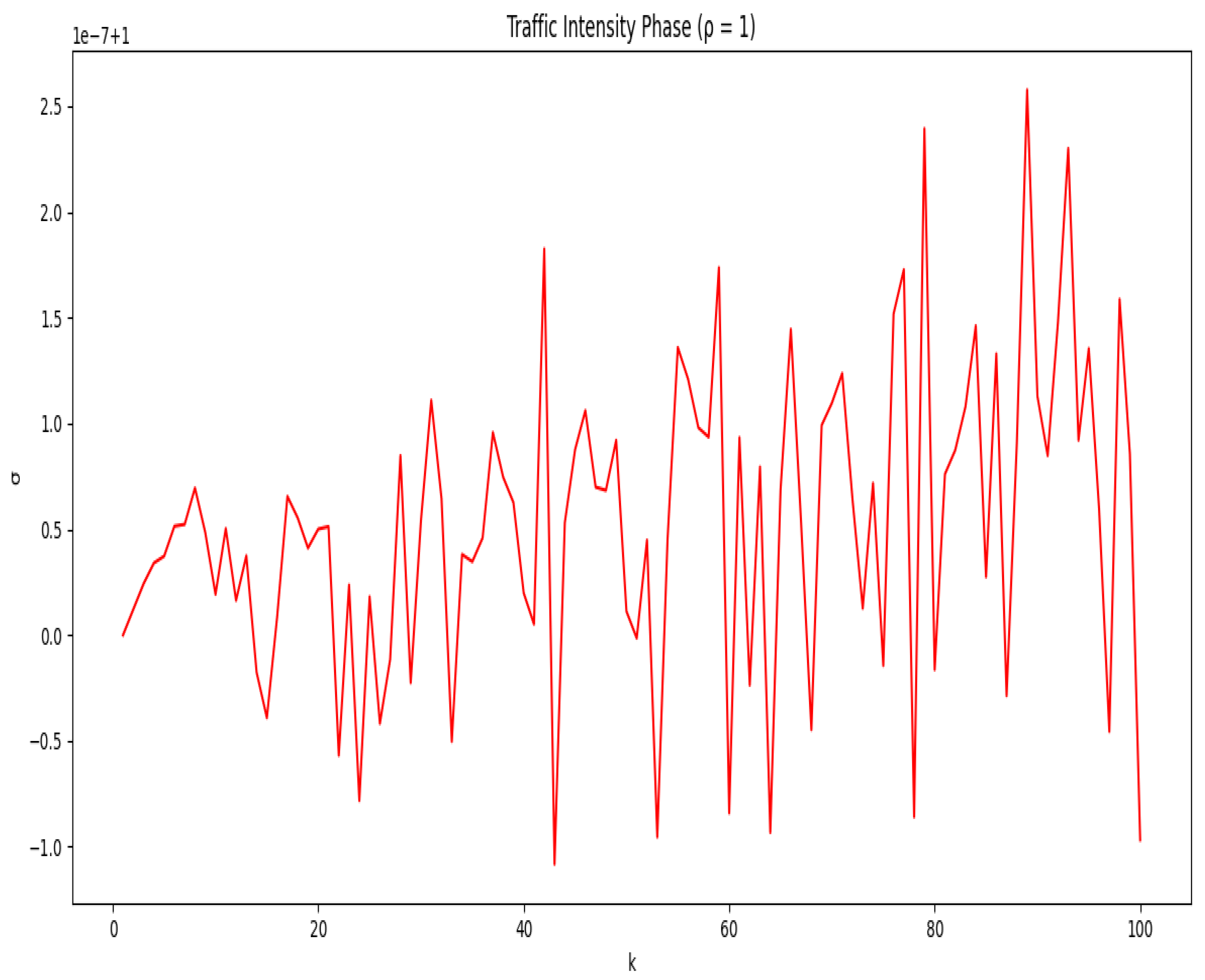
Looking closely at Figure 3, it is seen that for $k=\mathrm{1,2},\dots ,100$, the traffic intensity phase, namely, whenever we reach $\rho =1$, the root parameter $\sigma$ will follow the dual dynamics of stability and instability , which is a new phenomenon in PSFFA.

Chaotic Phase:

Figure 4. (Chaotic Phase 3D Plot): The plot reveals sharp, unpredictable variations in σ, indicating chaos as $\mathit{\rho }$ exceeds 1.

Figure 4. (Chaotic Phase 3D Plot): The plot reveals sharp, unpredictable variations in σ, indicating chaos as $\mathit{\rho }$ exceeds 1.

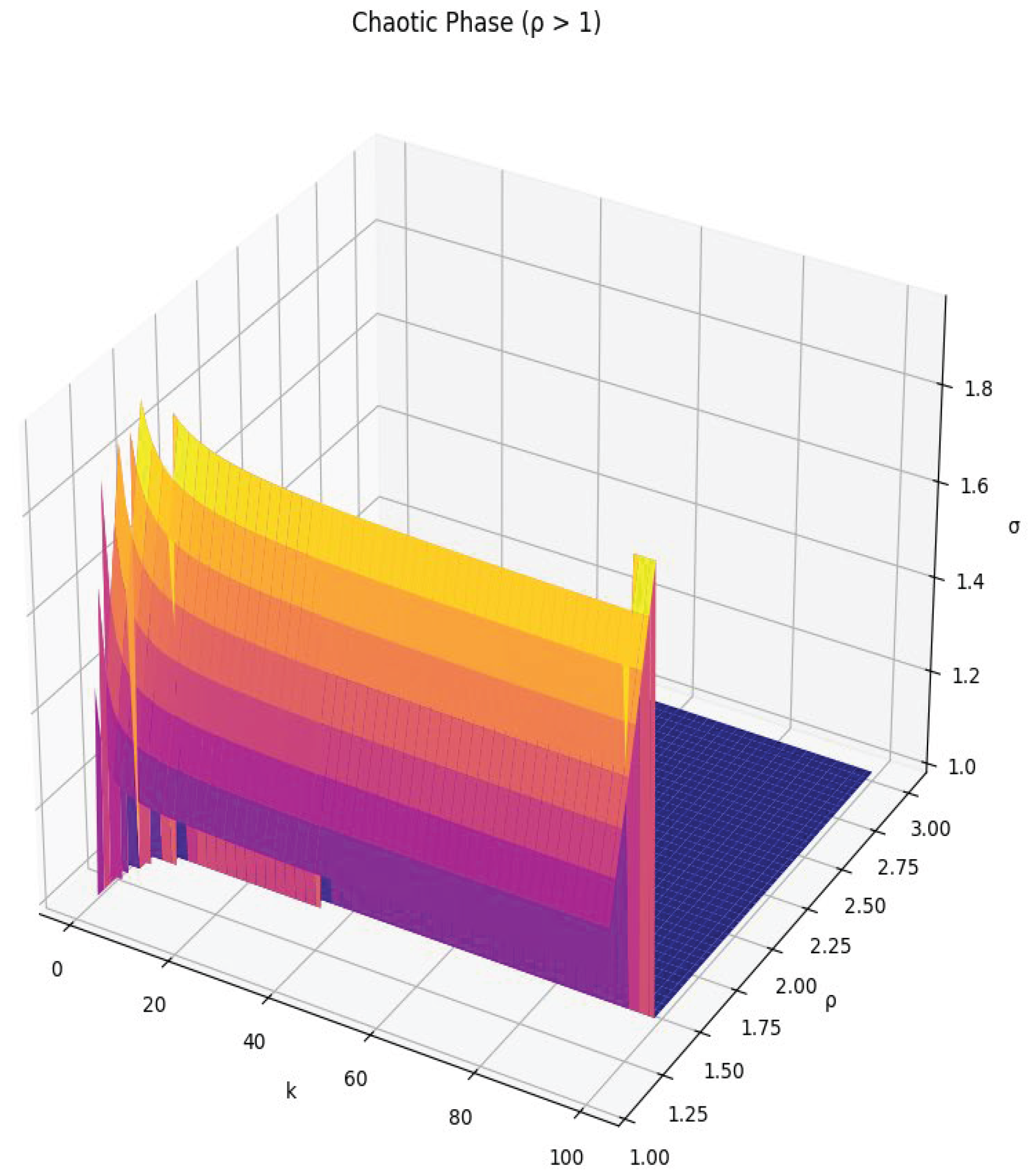
As for Figure 4, it is seen that for $\mathit{k}=\mathrm{1,2},\dots ,100$, the traffic intensity phase, namely, whenever we reach $\mathit{\rho }>1$, the root parameter $\sigma$ will follow the dynamics of instability, which is again another new phenomenon in PSFFA theory.

Comparison to Wei-Ping et al. (1996)

• Wei-Ping et al. (1996) provides an analytical model for nonstationary queues, focusing on steady-state approximations. Our work complements this by offering computational insights into transitions between stable and unstable phases.
• Unlike Wei-Ping et al. (1996), which assumes stationary behavior, our approach identifies conditions where chaos emerges (Wei-Ping et al., 1996).

Insights

• Critical Transitions: The stability phase is highly sensitive to small changes in ρ, whereas the chaotic phase exhibits larger, unpredictable variations.
• Algorithm Robustness: The iterative approach converges reliably under most conditions, with exceptions managed through error handling.

The current study has some limitations, such as the visualization of the unexplored dynamics at $k=\infty$. In other words, what are the mathematical and physical interpretations at sufficiently large values of $k$? This would be a next-generation vision of delving into a different universe within the approachability of infinity if it does exist as a number, not a mathematical concept (Leon, 2023) (Gutschmidt & Carl, 2024) (Nodelman & Zalta, 2024) to showcase our inability as mathematicians to count beyond a certain remit at the far edge of the counting spectrum. It is an informed guess of futuristic research into more explorations to solve this sophisticated open problem from mathematical and computational perspectives.

4. Conclusion Alongside Research Pathways

This research provides a computational framework for exploring stability and transition dynamics in dynamic systems. By iteratively approximating σ, we uncover critical insights into system behavior across stable, intense, and chaotic phases. The findings validate and extend the theoretical predictions by identifying new behaviours in chaotic systems. To accurately depict the transitions between these phases, the recent breakthrough uses computational techniques to visualize these connections for the undiscovered phenomenal negative values of the numbers of sets of phases, namely, k. In mathematical terms, the current explanation represents a new and amazing chapter in rethinking the entirety of PSFFA theory. It aims to move the long-unexplored subject of PSFFA into a higher level of thinking between disparate scientific disciplines, including chaos, quantum mechanics, random walks, Brownian motion, and much more. It is expected that, after examining the findings of this study, more research will be conducted on more untested situations to develop Ismail’s Contemporary PSFFA Theory and integrate it with a wide range of multidisciplinary fields of human knowledge. Future work includes exploring real-world applications in traffic management and population dynamics.

References

- Gutschmidt, R.; Carl, M. The negative theology of absolute infinity: Cantor, mathematics, and humility. International Journal for Philosophy of Religion 2024, 95(3), 233–256. [Google Scholar] [CrossRef]
- Leon, A. Infinity, Language, and non-Euclidean Geometries. The General Science Journal 2023, 173, 174, 1–5. [Google Scholar]
- Mageed, I. A. Effect of the root parameter on the stability of the Non-stationary D/M/1 queue’s GI/M/1 model with PSFFA applications to the Internet of Things (IoT). In Preprints: Preprints. 2024a. [Google Scholar]
- Mageed, I. A. The Infinite-Phased Root Parameter for the G1/M/1 Pointwise Stable Fluid Flow Approximation (PSFFA) Model of the Non-Stationary Ek/M/1 Queue with PSFFA Applications to Hospitals’ Emergency Departments. In Preprints: Preprints. 2024b. [Google Scholar]
- Mageed, I. A. Ismail’s Threshold Theory to Master Perplexity AI. Management Analytics and Social Insights 2024c, 1(2), 223–234. [Google Scholar] [CrossRef]
- Mageed, I. A. Solving the Open Problem of Finding the Exact Pointwise Stable Fluid Flow Approximation (PSFFA) State Variable of a Non-Stationary M/M/1 Queue with Potential Real-Life PSFFA Applications to Computer Engineering. 2024d. [Google Scholar] [CrossRef]
- Mageed, I. A. Upper and Lower Bounds of the State Variable of M/G/1 Psffa Model of the Non-Stationary m/Ek/1 Queueing System. Journal of Sensor Networks and Data Communications 2024e, 4(1), 1–4. [Google Scholar] [CrossRef]
- Mageed, I. A.; Zhang, K. Q. Solving the open problem for GI/M/1 pointwise stationary fluid flow approximation model (PSFFA) of the non-stationary D/M/1 queueing system. Electronic Journal of Computer Science and Information Technology 2023, 9(1), 1–6. [Google Scholar] [CrossRef]
- Nodelman, U.; Zalta, E. N. Number Theory and Infinity Without Mathematics. Journal of Philosophical Logic 2024, 53(5), 1161–1197. [Google Scholar] [CrossRef]
- Wei-Ping, W.; Tipper, D.; Banerjee, S. (1996, 24-28 March 1996). A simple approximation for modeling nonstationary queues. Proceedings of IEEE INFOCOM ‘96. Conference on Computer Communications. [CrossRef]
Disclaimer/Publisher’s Note: The statements, opinions and data contained in all publications are solely those of the individual author(s) and contributor(s) and not of MDPI and/or the editor(s). MDPI and/or the editor(s) disclaim responsibility for any injury to people or property resulting from any ideas, methods, instructions or products referred to in the content. |
© 2025 by the authors. Licensee MDPI, Basel, Switzerland. This article is an open access article distributed under the terms and conditions of the Creative Commons Attribution (CC BY) license (http://creativecommons.org/licenses/by/4.0/).
Copyright: This open access article is published under a Creative Commons CC BY 4.0 license, which permit the free download, distribution, and reuse, provided that the author and preprint are cited in any reuse.