
Submitted:
30 November 2024
Posted:
02 December 2024
You are already at the latest version
Abstract
This work explores the stability, traffic intensity, and chaotic phases in dynamic systems by iteratively approximating the sigma function (σ). Using Python as a computational tool, we calculate and visualize the relationship between parameters such as and . The analysis identifies transitions between stable and unstable phases, providing insights into system behaviour. Comparisons to foundational studies, has revealed novel contributions and validate the robustness of our algorithm. It is to be noted that, the current work provides new contributions to Ismail’s Contemporary Pointwise Stationary Fluid Approximation Theory, through offering a comprehensive computational framework for exploring dynamic system behaviours across varying parameters.
Keywords:
Pointwise Stationary Fluid Approximation(PSFFA)
; The non-stationary Ek/M/1 queue
; k sets of phases
1. Introduction
Understanding the stability and transition dynamics in complex systems is vital across domains like traffic management, population dynamics, and queueing theory. These systems exhibit various phases based on control parameters, including stability, intensity, and chaotic behaviour. Capturing these transitions mathematically and computationally remains a challenging yet essential task.
The foundational work in [1,2,3,4,5,6,7,8,9] provides a simplified approximation for nonstationary queues, laying the groundwork for dynamic system modelling. Building on this, we aim to refine the analysis by iteratively approximating the σ function, a measure of system response (σ), as a function of control parameters and .
Let and serve as the temporal flow in [1,2,3,4,5], and fow out, respectively. Therefore, by Equation (1)
For an infite queue waiting space, defined by Equation (3):
Thus (1) rewrites to Equation (4):
With
Where defines the number of set of phases,
Problem Definition
This study focuses on addressing the following phases:
- Stability Phase: Explore how σ changes for ρ ∈ [0.1, 0.999] and [1, 100].
- Traffic Intensity Phase: Examine system behaviour when ρ = 1 and [1, 100].
- Chaotic Phase: Investigate the system response for ρ > 1 (e.g., 2, 3, 4) and [1, 100].
Our approach utilizes computational tools to visualize these relationships, ensuring accurate representation of transitions between these phases.
Here is the structure of the current paper

2. Methodology
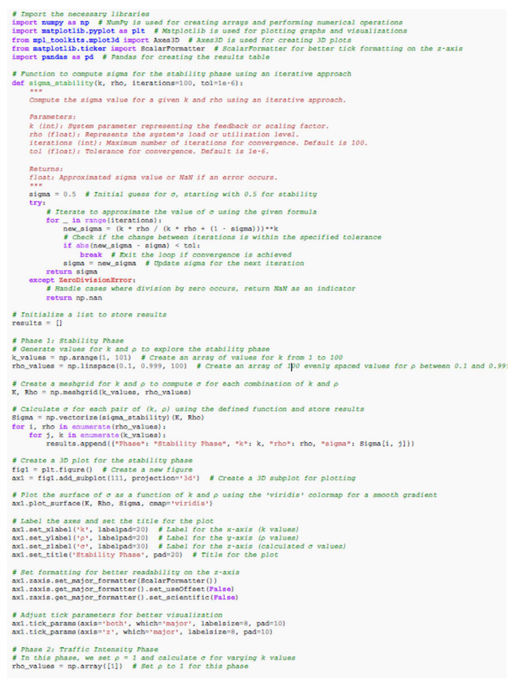
The computational framework is implemented in Python[10,11,12,13] leveraging libraries such as NumPy for numerical operations and Matplotlib for visualization. The iterative algorithm approximates σ using the formula (c.f., Equation (6)):
where σ is initialized to 0.5 and updated until convergence or reaching a tolerance of 10−6.
Key components of the algorithm include:
- Error handling for division by zero, ensuring robustness.
- Validation of results, checking for undefined outputs (e.g., NaN).
- Visualization of results in 2D and 3D plots.
Phases Overview
Stability Phase:
- Objective: Identify conditions where the system remains stable.
- Parameters: ρ ∈ [0.1, 0.999], k ∈ [1, 100].
- Visualization: 3D plots showing the surface of σ as a function of ρ and k.
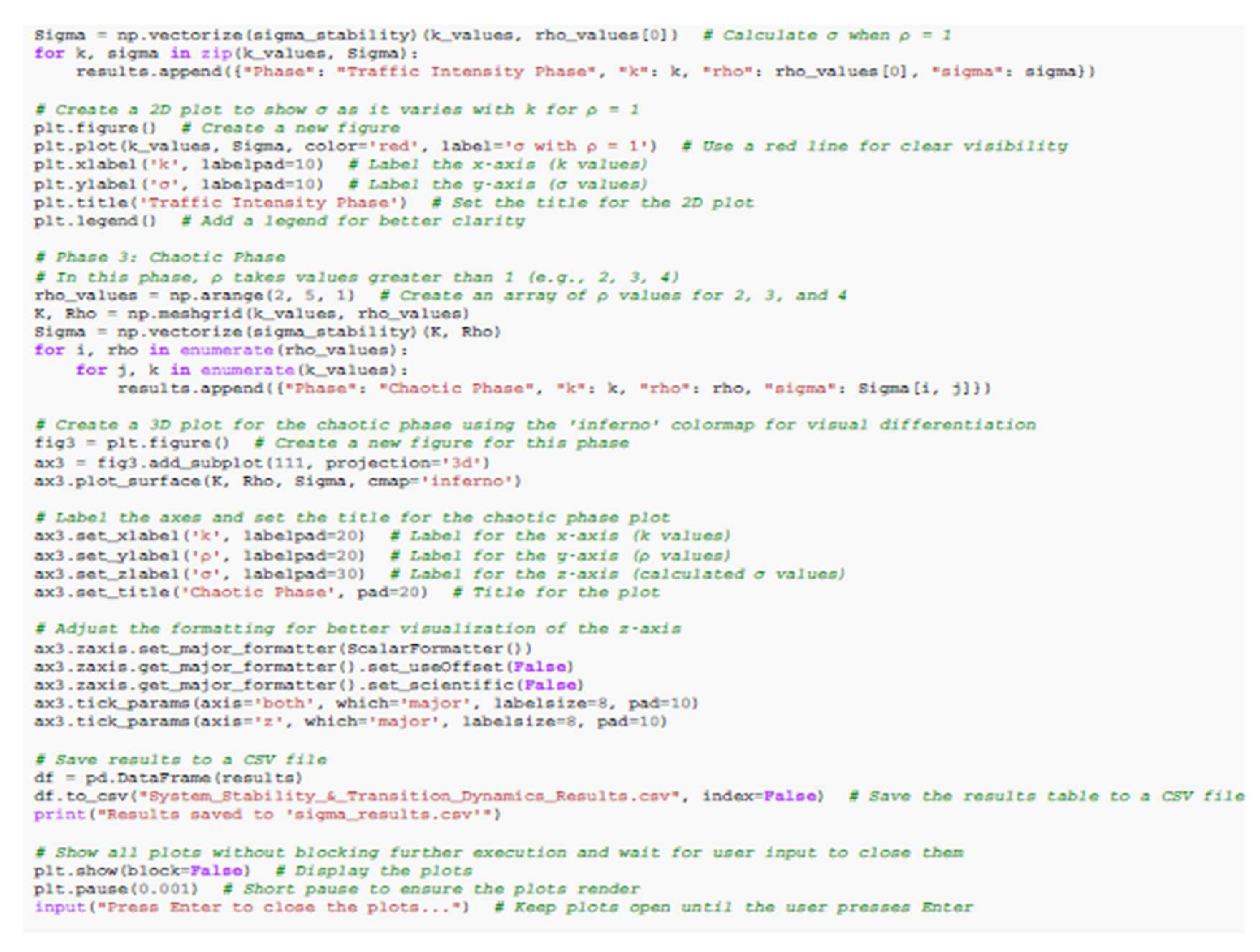
Traffic Intensity Phase:
- Objective: Analyse steady-state behaviour under maximum utilization (ρ = 1).
- Parameters: k ∈ [1, 100].
- Visualization: 2D plots of σ vs. k.
Chaotic Phase:
- Objective: Explore instability for ρ > 1 (e.g., 2, 3, 4).
- Parameters: ρ ∈ [2, 4], k ∈ [1, 100].
- Visualization: 3D plots highlighting unpredictable behaviour.
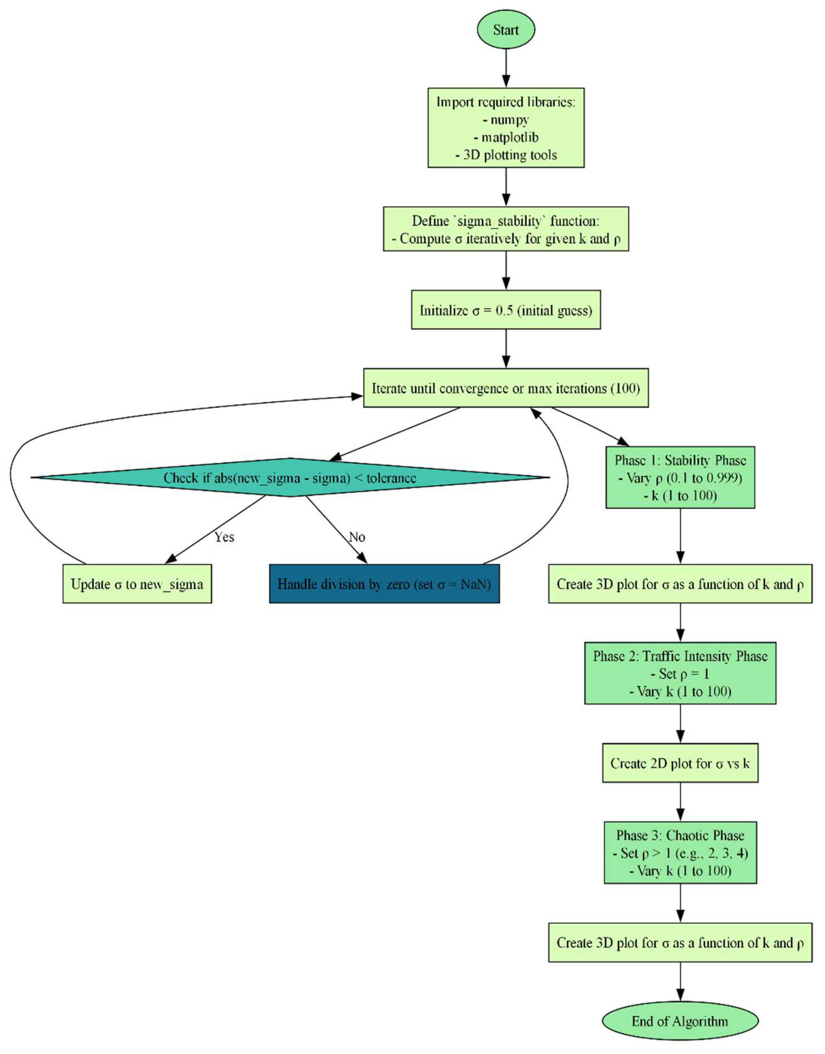
In what follows, the Pseudocode Diagram is visualized
Here is the source code of the program:
The pseudocode is structured as follows:
The algorithm for calculating the sigma (σ) values iteratively is illustrated below:
-
Import Libraries:
- The algorithm starts by importing necessary libraries such as NumPy and Matplotlib for numerical computation and visualization.
-
Define -stability Function:
- This function computes σ iteratively for given parameters k and ρ.
- Starting with an initial guess (), the function calculates updated values of σ until convergence or a maximum number of iterations (default 100).
-
Iterative Convergence:
- In each iteration, a new value of is computed using the formula:
- If the absolute difference between consecutive σ values is less than a specified tolerance (1e-6), the function exits, returning the converged value of σ.
-
Error Handling:
- A try-except block handles division-by-zero errors, ensuring the algorithm does not crash but returns NaN when such cases occur.
-
Iterate Over Phases:
- Stability Phase: Iterates over a range of ρ and k values to compute σ.
- Traffic Intensity Phase: Sets ρ = 1 (indicating maximum utilization) and computes how σ changes for varying values of k.
- Chaotic Phase: Explores the behaviour of σ for ρ > 1.
Explanation of Traffic Intensity Phase
The Traffic Intensity Phase models the system at maximum utilization ():
- Significance: This phase highlights how the system behaves under a fixed load condition. Unlike the stability phase, where ρ changes, the traffic intensity phase focuses solely on the effect of increasing k.
- Results: The algorithm computes σ for a range of k values (1 to 100) with ρ fixed at 1. This setup demonstrates saturation effects in the system, where σ stabilizes despite increasing k.
In the pseudocode, the traffic intensity phase is implemented as a separate loop that calculates and plots as a function of .
Here is the source code to generate Figures, 1,2 and 3
from graphviz import Digraph
def parse_python_to_flowchart():
# Create a directed graph for the flowchart
graph = Digraph(format=‘png’)
graph.attr(dpi=‘300’, rankdir=‘TB’, size=‘16,10’, margin=‘0.5’) # A4 landscape format
# Add nodes for the pseudocode
graph.node(“Start”, “Start”, shape=“ellipse”, style=“filled”, fillcolor=“#9AEBA3”) # Start node
# Algorithm explanation
graph.node(“Step1”, “Import required libraries:\n- numpy\n- matplotlib\n- 3D plotting tools”, shape=“box”, style=“filled”, fillcolor=“#DAFDBA”)
graph.node(“Step2”, “Define `sigma_stability` function:\n- Compute σ iteratively for given k and ρ”, shape=“box”, style=“filled”, fillcolor=“#DAFDBA”)
graph.node(“Step3”, “Initialize σ = 0.5 (initial guess)”, shape=“box”, style=“filled”, fillcolor=“#DAFDBA”)
graph.node(“Step4”, “Iterate until convergence or max iterations (100)”, shape=“box”, style=“filled”, fillcolor=“#DAFDBA”)
graph.node(“Step5”, “Check if abs(new_sigma - sigma) < tolerance”, shape=“diamond”, style=“filled”, fillcolor=“#45C4B0”)
graph.node(“Step6”, “Update σ to new_sigma”, shape=“box”, style=“filled”, fillcolor=“#DAFDBA”)
graph.node(“Step7”, “Handle division by zero (set σ = NaN)”, shape=“box”, style=“filled”, fillcolor=“#13678A”)
# Phase 1: Stability Phase
graph.node(“Phase1”, “Phase 1: Stability Phase\n- Vary ρ (0.1 to 0.999)\n- k (1 to 100)”, shape=“box”, style=“filled”, fillcolor=“#9AEBA3”)
graph.node(“Plot1”, “Create 3D plot for σ as a function of k and ρ”, shape=“box”, style=“filled”, fillcolor=“#DAFDBA”)
# Phase 2: Traffic Intensity Phase
graph.node(“Phase2”, “Phase 2: Traffic Intensity Phase\n- Set ρ = 1\n- Vary k (1 to 100)”, shape=“box”, style=“filled”, fillcolor=“#9AEBA3”)
graph.node(“Plot2”, “Create 2D plot for σ vs k”, shape=“box”, style=“filled”, fillcolor=“#DAFDBA”)
# Phase 3: Chaotic Phase
graph.node(“Phase3”, “Phase 3: Chaotic Phase\n- Set ρ > 1 (e.g., 2, 3, 4)\n- Vary k (1 to 100)”, shape=“box”, style=“filled”, fillcolor=“#9AEBA3”)
graph.node(“Plot3”, “Create 3D plot for σ as a function of k and ρ”, shape=“box”, style=“filled”, fillcolor=“#DAFDBA”)
# End node
graph.node(“End”, “End of Algorithm”, shape=“ellipse”, style=“filled”, fillcolor=“#9AEBA3”)
# Connect nodes
graph.edge(“Start”, “Step1”)
graph.edge(“Step1”, “Step2”)
graph.edge(“Step2”, “Step3”)
graph.edge(“Step3”, “Step4”)
graph.edge(“Step4”, “Step5”)
graph.edge(“Step5”, “Step6”, label=“Yes”)
graph.edge(“Step6”, “Step4”)
graph.edge(“Step5”, “Step7”, label=“No”)
graph.edge(“Step7”, “Step4”)
graph.edge(“Step4”, “Phase1”)
graph.edge(“Phase1”, “Plot1”)
graph.edge(“Plot1”, “Phase2”)
graph.edge(“Phase2”, “Plot2”)
graph.edge(“Plot2”, “Phase3”)
graph.edge(“Phase3”, “Plot3”)
graph.edge(“Plot3”, “End”)
return graph
# Main script
if __name__ == “__main__”:
# Generate the flowchart
flowchart = parse_python_to_flowchart()
# Render the flowchart as a PNG file
output_path = “System_Stability_&_Transition_Dynamics_Flowchart”
flowchart.render(output_path, format=“png”, cleanup=True)
print(f”Flowchart saved as ‘{output_path}.png’“)
3. Results and Analysis
Visualization
Stability Phase:
Data Snippets
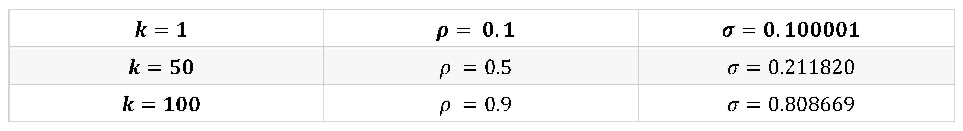
As showcased by Figure 1, it is seen that for , the stability phase, adhering , the root parameter will follow the dynamics of stability.
Traffic Intensity Phase:
Data Snippets

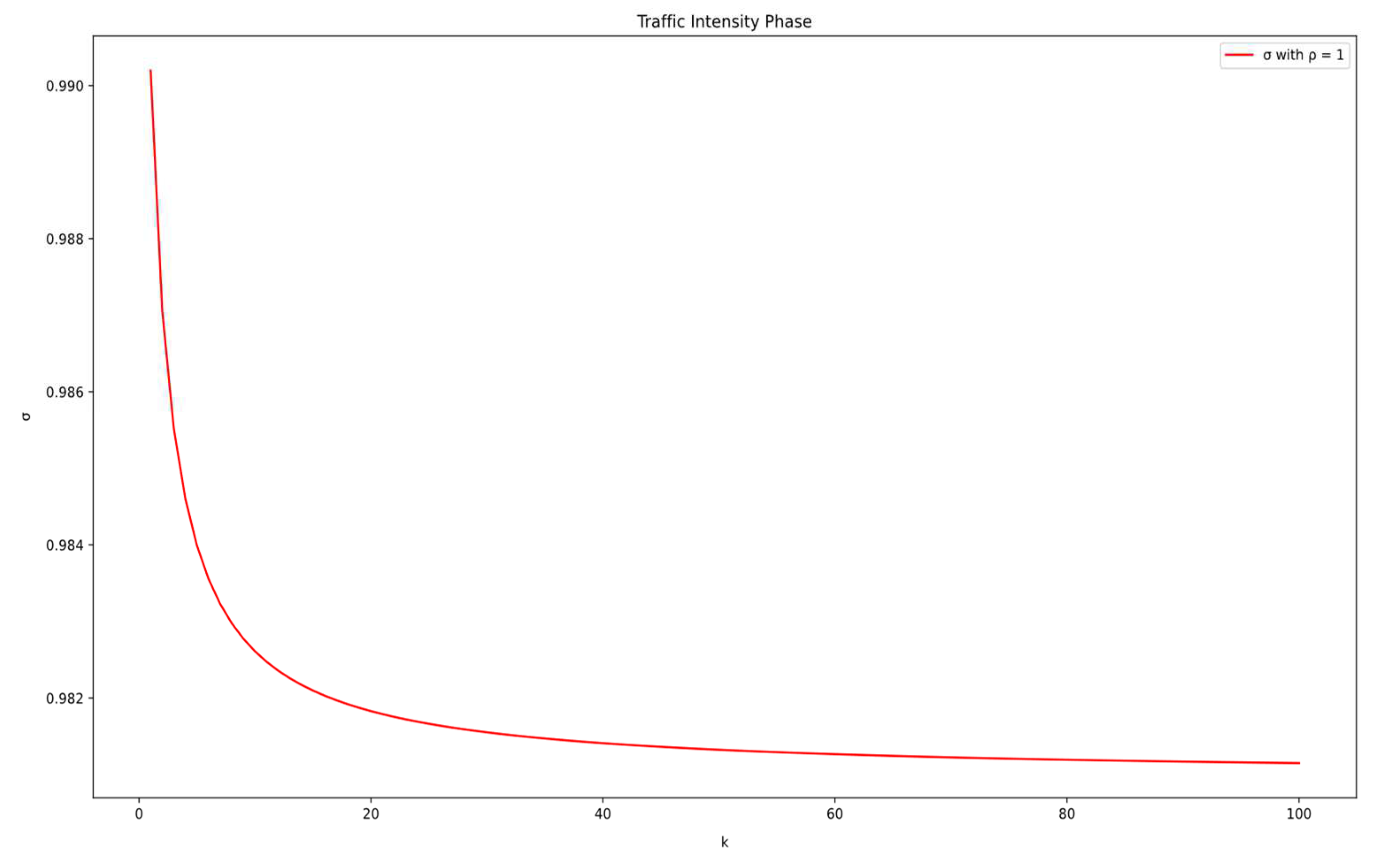
Looking closely at Figure 2, it is seen that for , the traffic intensity phase, namely, whenever we reach , the root parameter will follow the dynamics of stability, which is a new phenomenon in PSFFA.
Chaotic Phase:
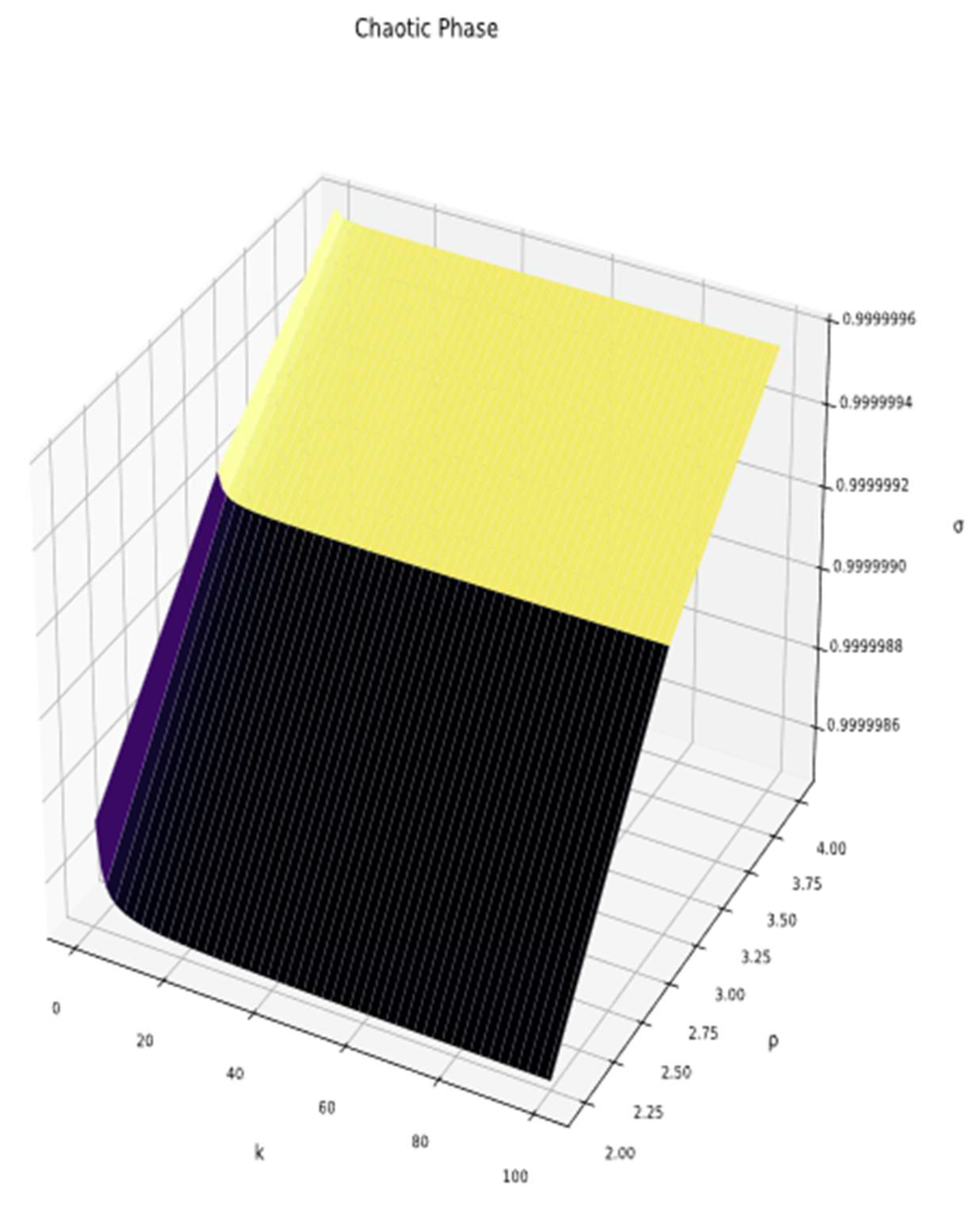
Figure 3 (Chaotic Phase 3D Plot): The plot reveals sharp, unpredictable variations in σ, indicating chaos as exceeds 1.
Data Snippets

As for Figure 3, it is seen that for , the traffic intensity phase, namely, whenever we reach , the root parameter will follow the dynamics of stability, which is again another new phenomenon in PSFFA theory.
Comparison to [14]
- [14] provides an analytical model for nonstationary queues, focusing on approximations for steady states. Our work complements this by offering computational insights into transitions between stable and unstable phases.
- Unlike [14], which assumes stationary behaviour, our approach identifies conditions under which chaos emerges.
Insights
- Critical Transitions: The stability phase is highly sensitive to small changes in ρ, whereas the chaotic phase exhibits larger, unpredictable variations.
- Algorithm Robustness: The iterative approach converges reliably under most conditions, with exceptions managed through error handling.
4. Conclusion Alongside Research Pathways
This research provides a computational framework for exploring stability and transition dynamics in dynamic systems. By iteratively approximating σ, we uncover critical insights into system behaviour across stable, intense, and chaotic phases. The findings not only validating the theoretical predictions , but also extend them by identifying new behaviours in chaotic systems.
Future work includes:
- Extending the analysis to all real values of , as hinted at in the unexplored negative values of .
- Exploring real-world applications in traffic management and population dynamics
References
- Mageed,I., A.(2021). Solving the unsolvable the closed form solution of PSFFA model of non-stationary queueing systems, DEAMN 2021, Online Yarmouk University Mathematics conference, Jordan, 2021.
- Mageed, I. A., & Zhang, K. Q. (2023). Solving the open problem for GI/M/1 pointwise stationary fluid flow approximation model (PSFFA) of the non-stationary D/M/1 queueing system. electronic Journal of Computer Science and Information Technology, 9(1), 1-6. [CrossRef]
- Mageed, I. A, Babagana, M, closed form analytic solution for GI/M/1 pointwise stationary fluid flow approximation model (PSFFA) of the non-stationary D/M/1 queueing system, Conference of the Southern Africa Mathematical Sciences Association - SAMSA2021 November 22 - 24, 2021, Virtual Conference.
- Mageed,I., A (2024).Effect of the root parameter on the stability of the Non-stationary D/M/1 queue’s GI/M/1 model with PSFFA applications to the Internet of Things (IoT). Preprints 2024, 2024011835. [CrossRef]
- Mageed,I., A .(2024)Solving the Open Problem of Finding the Exact Pointwise Stable Fluid Flow Approximation (PSFFA) State Variable of a Non-Stationary M/M/1 Queue with Potential Real-Life PSFFA Applications to Computer Engineering, 28 January 2024, PREPRINT (Version 1) available at Research Square. [CrossRef]
- Mageed,I., A .2024) Upper and Lower Bounds of the State Variable of M/G/1 PSFFA Model of the Non-Stationary M/Ek/1 Queueing System. Preprints 2024,2024012243. [CrossRef]
- Mageed,I., A. (2024) The Infinite-Phased Root Parameter for the G1/M/1 Pointwise Stable Fluid Flow Approximation (PSFFA) Model of the Non-Stationary Ek/M/1 Queue with PSFFA Applications to Hospitals’ Emergency Departments. Preprints 2024, 2024021021. [CrossRef]
- Mageed,I., A. (2024). Upper and Lower Bounds of the State Variable of M/G/1 PSFFA Model of the Non-Stationary M/EK/1 Queueing System. J Sen Net Data Comm, 4(1), 01-04. [CrossRef]
- Mageed,I., A. (2024). Effect of the Root Parameter on the Stability of the Non-Stationary D/M/1 Queue’s GI/M/1 Model with PSFFA Applications to the Internet of Things. J Sen Net Data Comm, 4(1), 01-09.
- Python, W. (2021). Python. Python releases for windows, 24.
- Weerakoon, L., Herr, G. S., Blunt, J., Yu, M., & Chopra, N. (2022). Cartographer_glass: 2D graph SLAM framework using LiDAR for glass environments. arXiv preprint arXiv:2212.08633.
- Virtanen, P., Gommers, R., Oliphant, T. E., Haberland, M., Reddy, T., Cournapeau, D., ... & Van Mulbregt, P. (2020). SciPy 1.0: fundamental algorithms for scientific computing in Python. Nature methods, 17(3), 261-272. [CrossRef]
- D’Amico, M., Morasca, P., Spallarossa, D., Bindi, D., Picozzi, M., & Vitrano, L. (2024). User Manual of GITpy: a Python-based tool for the Generalized Inversion Technique. Rapporti Tecnici-INGV.
- Wang, W. P., Tipper, D., & Banerjee, S. (1996, March). A simple approximation for modelling nonstationary queues. In Proceedings of IEEE INFOCOM’96. Conference on Computer Communications (Vol. 1, pp. 255-262). IEEE.
Figure 1.
(Stability Phase 3D Plot): The surface plot shows a gradual increase in σ as ρ and k increase. This highlights regions of stability under varying conditions.
Figure 1.
(Stability Phase 3D Plot): The surface plot shows a gradual increase in σ as ρ and k increase. This highlights regions of stability under varying conditions.
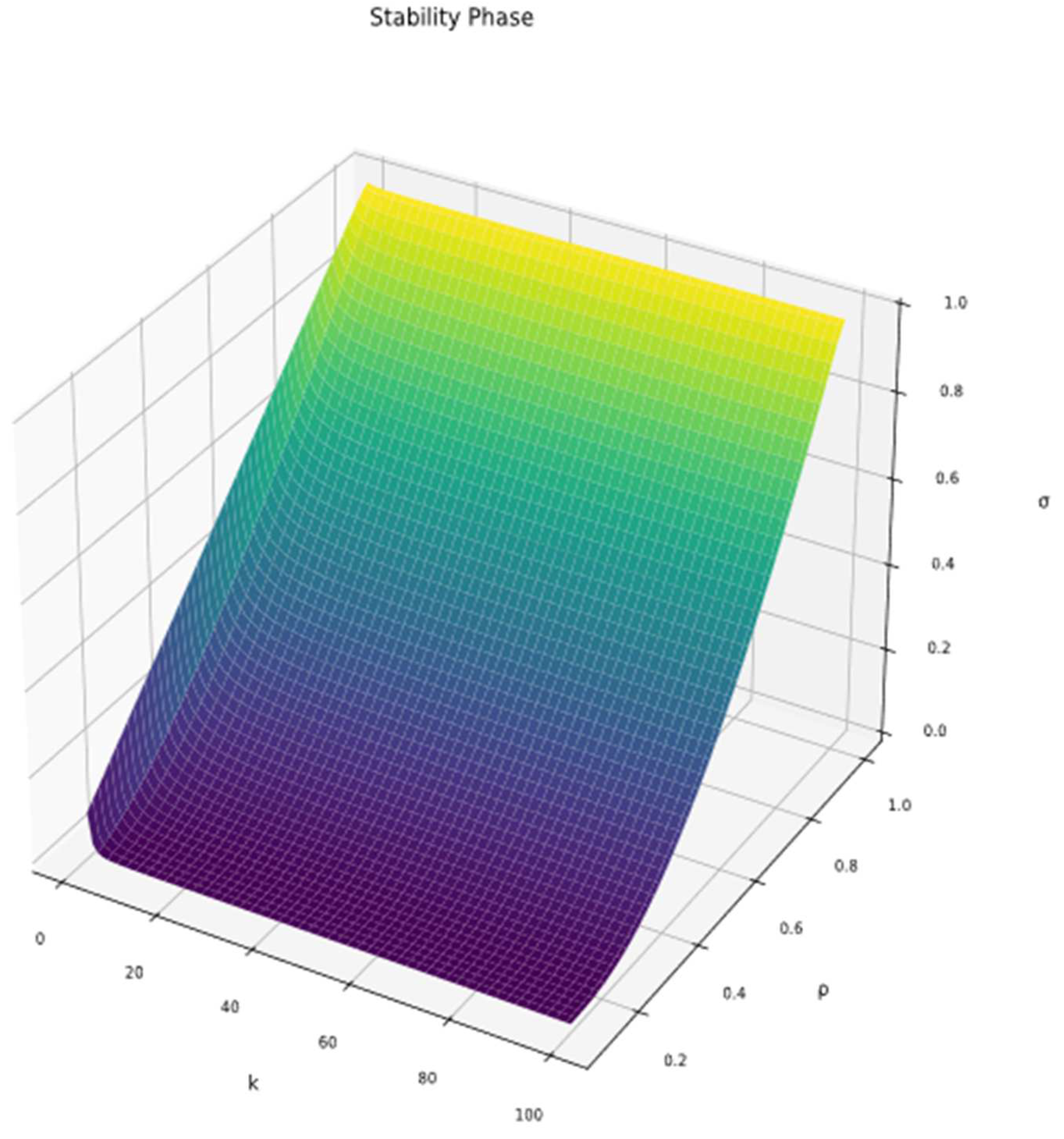
Figure 2.
(Traffic Intensity Phase 2D Plot): The curve demonstrates a saturation effect, where approaches a constant value as increases.
Figure 2.
(Traffic Intensity Phase 2D Plot): The curve demonstrates a saturation effect, where approaches a constant value as increases.
Disclaimer/Publisher’s Note: The statements, opinions and data contained in all publications are solely those of the individual author(s) and contributor(s) and not of MDPI and/or the editor(s). MDPI and/or the editor(s) disclaim responsibility for any injury to people or property resulting from any ideas, methods, instructions or products referred to in the content. |
© 2024 by the authors. Licensee MDPI, Basel, Switzerland. This article is an open access article distributed under the terms and conditions of the Creative Commons Attribution (CC BY) license (http://creativecommons.org/licenses/by/4.0/).
Copyright: This open access article is published under a Creative Commons CC BY 4.0 license, which permit the free download, distribution, and reuse, provided that the author and preprint are cited in any reuse.


