
Submitted:
02 February 2023
Posted:
03 February 2023
You are already at the latest version
Abstract
Self-organized criticality (SOC) is a celebrated paradigm from the 90’s for understanding dynamical systems naturally driven to its critical point, where the power-law dynamics taking place make predictions practically impossible, such as in stock prices, earthquakes, pandemics and many other problems in science related to phase transitions. Shortly thereafter, it was realized that traffic flow might be in the SOC category, implying that conventional traffic management strategies seeking to maximize the local flows can become detrimental. This paper shows that the Kinematic Wave model with triangular fundamental diagram, and many other related traffic models, indeed exhibit SOC, thanks in part to the fractal nature of traffic exposed here on the one hand, and our need to get to our destinations as soon as possible, on the other hand. Important implications for congestion management of traffic near the critical region are discussed, such as: (i) Jam sizes obey a power-law distribution with exponent 1/2, implying that both its mean and variance become ill-defined and therefore impossible to estimate. (ii) Traffic in the critical region is chaotic in the sense that predictions becomes extremely sensitive to initial conditions. (iii) However, aggregate measures of performance such as delays and average speeds are not heavy tailed, and can be characterized exactly by different scalings of the Airy distribution, (iv) Traffic state time-space “heat maps” are self-affine fractals where the basic unit is a triangle, in the shape of the fundamental diagram, containing 3 traffic states: voids, capacity and jams. This fractal nature of traffic flow calls for analysis methods currently not used in our field.
Keywords:
traffic flow
; kinematic wave model
; self-organized criticality
; fractals
; complexity
; catastrophe theory
; non-equilibrium critical phenomena
1. Introduction
There is mounting empirical evidence [1,2,3] suggesting the hypotheses that urban networks exhibit self-organized criticality (SOC) [4], a celebrated paradigm in the 90’s that has proved very useful in countless areas of science, from earthquakes to stock prices to forest fires to astrophysics [5,6]. Despite being around for 2 or 3 decades now, the theory and control consequences of SOC–and the corresponding fractal nature of traffic flow–have not permeated the transportation engineering literature, and even in the physics literature these concepts are only acknowledged but not exploited [7,8,9,10]. This is unfortunate because if it turns out that urban networks do exhibit SOC, a whole new paradigm emerges for understanding urban congestion, based on the lessons learned from complexity, catastrophe theory and non-equilibrium critical phenomena [11].
But given the absence of a general theory of SOC to date [6], it is not yet possible to formally prove or disprove this hypothesis. This paper is a step towards such a theory for traffic flow. The defining characteristic of a SOC system is that it is naturally driven to be in a “critical state” where it undergoes a phase transition [12] (e.g. from liquid to solid or from free-flow to congestion). At the critical point the characteristic length scale of the system, such as the size S of forest fires or the size of traffic jams as shown here, diverges to infinity, which renders the system scale-free and thus scale invariant. This implies a power-law distribution for the jam size, whose tail probability is proportional to , i.e.:
with the exponent known as the critical exponent. As opposed to the normal distribution, where it is virtually impossible to find realizations more than 3 standard deviations away from the mean value, power laws are said to have “heavy tails”: there is a non-negligible probability of observing extremely large values. As a consequence, the moments of the distribution may not exist, in which case the central limit theorem and the law of large numbers no longer hold. When , both the mean and variance are finite; when , as it is typically the case, the mean is finite and the variance diverges, and for both the mean and variance diverge. The case is popularly known as Zipf’s law [13], and as it turns out for a wide variety of phenomena, from the floods of the Nile River [14] to the population of cities [15], earthquake magnitudes, allometric scaling in mammals [16], word frequencies [13], reference links on the web [17], financial returns [18], the size (number of employees, sales, assets) of companies [19,20], turbulent flows and many others [21].
SOC behavior in traffic flow models has been conjectured since the mid-nineties in the physics community [22,23]. Using ideas from the theory of percolation phase transitions and the [24] cellular automata model (NaSch model) for numerical experiments, they conjectured that (i) the critical exponent of jam durations in (1) is very close to 1/2, suggesting a relationship with the first return time of a one-dimensional random walk, and (ii) the number of vehicles under congestion scales with time as . They conclude that SOC implies that conventional traffic management strategies seeking to maximize the flow may be detrimental as they make the system more unpredictable and hard to control. Here, we will formalize conjecture (i) using the variational theory of traffic flow [25], and point out that the scaling in (ii) is in fact . We will also argue that current control strategies could be adapted to minimize the externalities of SOC by ensuring the network density always remains well below the critical density.
Surprisingly, the impact of SOC in our field has been underwhelming [26,27]. Apart from [28,29,30] who present some numerical evidence of SOC on networks, it appears that the subject has gone largely under the radar. One reason might be that the main insight from the early works [22,23] was that SOC in the NaSch model emerges only in ”cruise-control” mode, where random perturbations are only allowed in congested traffic states. This apparent dependence on the rule details might have been interpreted as the absence of a universality class in traffic flow, implying that SOC might not be an intrinsic property of traffic flow, but just of particular models.
This paper shows that the Kinematic Wave model [31,32] with triangular fundamental diagram, and many other related traffic models including the NaSch model, indeed exhibit SOC. In our case, showing SOC comes down to showing that (i) there is critical behavior at the transition between free-flow and congestion, and (ii) the system has a tendency to be in the critical state. The paper focuses on (i) because (ii) follows immediately from our willingness to drive as fast as possible, which translates into the well-known entropy solution of the kinematic wave model where e.g. the outflow after the signal turns green is maximized precisely at the critical density.
The remainder of the paper is organized as follows. Section 2 below establishes the equivalence of foundational traffic models in the literature. Section 3 shows that a mathematical cause for criticality in traffic flow is provided by variational theory with random initial conditions around the critical density, which produces power-law statistics for jam durations and spans. Section 4 presents aggregate measures of performance such as total delay, total distance traveled, average flows and speeds, and probability of congestion. Note that these measures of performance are not heavy tailed, and are related to the area under a random walk. A discussion and outlook is provided in the last section.
2. Equivalence of Traffic Flow Models
This section recalls existing results demonstrating that a large family of well-known traffic flow models, both continuum and discrete, are fundamentally equivalent. This is important because it allows us to use existing knowledge behind each of these models to the benefit our understanding of a single theory, best known to this community as the the kinematic wave theory of [31,32] with triangular fundamental diagram.
A microscopic formulation of this theory is the celebrated Newell’s car-following model [33], which can in turn be formulated as a cellular automaton (CA) [34]. The NaSch model, for which critical behavior was first conjectured, is a stochastic version of Daganzo’s CA model that introduces bounded acceleration and a probability of slow down for moving vehicles.
Another important known result is that the particular values of the slopes of the fundamental diagram are irrelevant because one can always transform the output of a traffic model with a particular diagram to the output from a different diagram via simple linear transformations; see [35]. This means that, effectively, traffic flow on a single link requires no parameters (after proper normalization). Therefore, and without loss of generality, in this paper we will use an isosceles flow-density fundamental diagram, which has the virtue, among others [35], of turning Daganzo’s CA model in to elementary cellular automata rule 184 [36], namely ECA 184, by using the following parameters:
These parameters imply that both the capacity and the critical density are 1/2, that distances are measured in units of one vehicle length and that time is measured in units of 1/2 of a critical headway.
All the models in this section will be collectively referred to as “the traffic model” in what follows. The focus of this paper is on showing the critical behavior of the deterministic traffic model rather than the random NaSch model. In this way, it can be established that critical behavior does not require random traffic rules, only random initial data.
3. The Root Cause of Criticality in Traffic Flow
In this section we show that the deterministic traffic model exhibits critical dynamic behavior under random initial conditions around the critical density. This is achieved using the Variational Theory of traffic flow [25], which boils the traffic flow problem down to a minimum path problem. It turns out that around the critical density this minimum path problem is intimately related to the theory of random walks, whose return times are power-law distributed.
The basic experiment in this paper is a single-lane road segment of length L with with vehicles obeying the deterministic traffic model and starting with initial density conditions at the critical density of 1/2 plus a random noise. For the continuum traffic models the random noise is interpreted here as a white noise process, i.e. initial density fluctuations at any location are assumed independent of one another and follow the standard normal distribution. For the equivalent discrete models, where the road segment is divided into L cells of jam-spacing size, the random noise becomes a Bernoulli process over the cells , which can be either 0 (empty) or 1 (occupied by a vehicle) with probabilities 1-p and p, respectively, independently of other cells. Notice that p can also be interpreted as the mean density in the segment, so .
The central contribution of this paper is made possible using Variational Theory, which is based on the traffic flow surface, , that gives the cumulative vehicle number having crossed location x by time t starting from the passage of a reference vehicle. The spatial integration of the continuum and discrete processes described above are examples of the Brownian motion and random walk processes, respectively, which have played a central role in arguably all areas of science and therefore many exact analytical results are known. In our case the Brownian motion/random walk correspond to the initial conditions , which is given by the (negative) integral of the initial density. In Variational Theory, the very existence of the fundamental diagram becomes a Hamilton-Jacobi partial differential equation (PDE) [37], whose solutions can be found by solving the shortest path problem:
known as the Hopf-Lax formula [38]. The fundamental diagram corresponds to the Hamiltonian of the system, whose corresponding Lagrangian is denoted and gives the maximum passing rate of an observer moving at a given speed. The shortest path problem consists in finding a trajectory from to the initial (and/or boundary) data at that minimizes the total cost along the path, given by the term in brackets, satisfying , and , since represents a wave speed. For a homogeneous facility (where the fundamental diagram does not change) the Lagrangian becomes independent of space and time, the time integral in (3) simplifies to where y is now a scalar satisfying . Accordingly, to find the solution at a generic time-space point amounts to finding the minimum straight-line path from to the initial boundary at , where the cost of each path is , with . In the case of the isosceles fundamental diagram used here, and (3) simplifies to:
where , and define the extent of the search interval; see points U and D in Figure 1. With deterministic initial conditions at the critical density we have and the cost function becomes which is independent of y. Therefore, all paths from P to the boundary are optimal (since they all have the same cost) and we let
be this deterministic solution. The important point here is that this nature of the solution holds even when a white noise is added to the initial densities. In this case, becomes a Brownian motion with zero drift, which revolves around a constant (independent) expected value:
As shown next, this result implies that the lifetime of traffic jams exhibits critical behavior.
3.1. Lifetime of Elementary Jams
Let an elementary jam be a line segment in the ()-plane that starts at a congested point D on the initial boundary and proceeds upstream at the congested wave speed so long as the visited cells are congested/occupied; see Figure 1. This is akin to a characteristic line segment connecting D to P but only passing through congested points in the plane and ending when reaching an empty cell. Ending points such as P in the figure are characterized by a transition from free-flow to congestion at that point, which means that the cost of minimum paths P-U and P-D in the figure both solve (4) and therefore have identical cost, i.e. . This means that the duration in Figure 1 is given by the first return time of our Brownian motion , i.e. the time it takes for the Brownian motion starting at U to “return” to the same value. These return times are known to have a power law distribution with exponent 1/2 [see e.g. [39], p.152]. From Figure 1 it is clear that the duration, H, of an elementary jam is and therefore retains the same power-law distribution with exponent 1/2:
The consequences of this are far-reaching: both the mean and variance of elementary jam durations and distance traveled diverge (to infinity on a ring road, and to values proportional to the system size on a finite road), which renders standard statistical tools inadequate. Most notably, the law of large numbers does not apply: taking a sample of jam durations to estimate mean and variance is futile because these estimates will not converge regardless of the sample size.
3.1.1. Jam sizes
Let us define a jam as a congestion cluster in the time-space () plane, i.e. a ()-region where all vehicles are stopped. In terms of elementary jams, a jam can be characterized by a collection of, say n, of contiguous elementary jams. Turning to the discrete version of our problem for simplicity, the size S of a jam can be written as:
where the ’s are elementary jam durations conditioned on being greater than the previous one. To see this, consider the duration in Figure 1. One can see that the duration of the elementary jam above it, , which is part of the same jam, is smaller than and therefore . Since the conditional distribution is also a power law with the same exponent, 1/2 in this case, one can expect S to also obey the same power law, regardless of the value of n [40]. We conclude:
which has been verified numerically; see inset in Figure 1. The experiment in the figure consistent in evolving ECA-184 for time periods starting with an initial row of cells, each with a probability of being occupied. The time-space area for cluster measurement is of triangular shape as in Figure 1, where to ensure that all points in A are able to reach the boundary. The jam sizes were plotted on a log-log plot so that the slope of the linear segment gives the exponent of the power law.
3.1.2. Exponent Near the Critical Density
To study the behavior near the critical density, we expand the experiment above to include a range of mean initial densities p. Figure 2 shows the relationship between the estimated power-law exponent and p in our experiment for . The downwards trend is fairly linear around the critical density, as in second-order phase transitions, and can be described approximately as
The sizable but decreasing interval width of the transition, at the critical density, is a strong indication that the exponent that best describes a particular realization is highly sensitive to the initial conditions. This makes prediction challenging, especially considering that is a fairly large road segment of around 10 kilometers, and that the interval width increases for smaller segments, e.g. for as seen in Figure 2.
It is important to note that only near the critical density these power-law exponent are meaningful. Figure 2 (Bottom) shows 3 detailed outputs for selected values of p, where one can see that for there is a clear power law relationship but with a very limited range, because in the free-flow jams are very small. For for the cluster distribution describes a piecewise-linear relationship, as a consequence of several clusters “percolating” to the opposite side of the triangle in the time-space plane.
4. Aggregate Measures of Performance during the Transition to Equilibrium
This section uses the results from section 3 to derive the distribution of delays, flows and speeds aggregated during the initial period where the system studied here relaxes to equilibrium. This relaxation time T was shown to be [41] for ECA 184 under the same random initial conditions in this paper, and therefore we only need to analyze the system for T time units. The time-space region for analysis in this section is taken as a triangle of area as in Figure 1, which defines all the points that may be affected by the initial conditions according to variational theory. In this way, our results are not restricted to a ring road and also apply to a typical roadway segment.
4.1. Delay, Flow and Speed
Let and be the total time traveled and total distance traveled, respectively, over a (discrete) time-space region A. By letting the symbol A also denote its area, Edie’s [42] average density, flow and speed in and , respectively, are given by:
These general definitions can be greatly simplified in our case because the spatiotemporal solution to our problem only involves 3 traffic states: capacity state C with (flow, density) = (1/2, 1/2), the empty or void state O with (0,0) and the jam state J with (0, 1). The total area that each state occupies in A is indicated with a subscript, and they satisfy:
Notice that the total delay experienced by drivers inside A is equal to . This is because is the only area where vehicles experience congestion and all the time inside this area is a delay (since they are stopped). The total travel time , and the total distance traveled . Using (12) we have:
and therefore the total delay is bounded. Also,
where correspondence to the probability that a time-space point in A is congested. Perhaps unsurprisingly, it can be seen that the total total delay turns out to be the key measure of performance from which all others can be derived.
4.2. Moments and Probability Densities
The main result here is that for an area of triangular shape as in Figure 1, the the total delay corresponds to half the area under a Brownian excursion, :
A Brownian excursion is a conditioned one-dimensional Brownian motion over the interval such that its path starts and ends at the origin and it is constrained to stay positive in between. It is important to note that the area under the excursion is also given by the area between a Brownian bridge and its minimum value in . This second interpretation is precisely our context: (i) exactly at the critical density the number of empty and unoccupied cells are equal so that in our random walk , which corresponds to a Brownian bridge, and (ii) from Figure 1 it can be seen that (half) the total area under the random walk and its minimum value is , since by definition we have:
where m is the total number of elementary jams in the system. Unlike (8), the correlations among the ’s in (16) play a significant role here because the sum across all elementary jams in the system is limited by the size of the system itself, and therefore its distribution will not be a power law, as shown next.
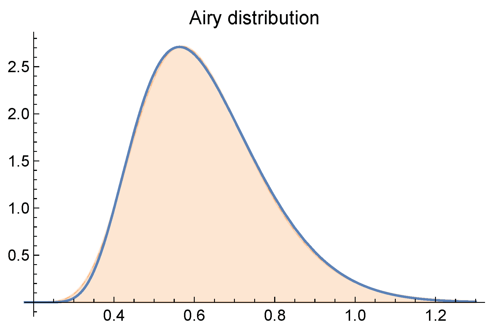
For the unit length road segment the area under a Brownian excursion, is known to have the Airy distribution [43,44,45]; let be its PDF. Figure 3 plots the PDF of the Airy distribution, . Notice that it is not a heavy-tail distribution; [44] shows that its mean and standard deviation are given by Although the Airy distribution is not exactly symmetric, one can approximate the interval where most of the realizations of Z would fall: .
Given the self-similarity properties of Brownian motions, we have that has the same distribution as [43], and therefore is an invariant quantity in our problem. Most of the realizations of would fall in the interval . Similarly, the invariant probability of congestion is and has the same distribution as . Importantly, it also follows that:
To correctly interpret these insights, which are not contradictory, recall that the analysis area changes with the size of the segment. Therefore, doubling the size of the road increases the analysis area by a factor of 4, but the total delay only by a factor of , implying economies of scale. It is not surprising then, that the probability of congestion actually decreases by a factor of .
To obtain the PDF of the total delay one can use the above self-similarity arguments to show that
The distribution of all other traffic flow variables will be given by different scalings of the Airy distribution. It follows from (14) that the PDFs for these variables are given by
which only depend upon .
5. Discussion and Outlook
This paper has presented strong evidence that traffic flow in individual road segments exhibits all the characteristics of critical systems subject to SOC. We have seen that this critical behavior can be traced back to the deep connection with Brownian motions formalized here thanks to the variational theory of traffic flow, establishing that even though the traffic rules are perfectly deterministic, the randomness encoded in the initial conditions is enough to generate power-law dynamics during the transient to equilibrium. Adding our willingness to maximizes travel speeds establishes SOC for the deterministic traffic flow models analyzed in this paper. We are therefore in a position now to accept Nagel and Paczuki’s 1995 conjecture that traffic management strategies seeking to maximize flow are bound to cause more harm than good.
An effective control premise appears to be to prevent the density from reaching the critical region, e.g. by metering well below capacity or congestion pricing. Research is needed to devise an analytical framework able to cope with the difficulties imposed by the type of power-laws-from-fractal dynamics with exponent less than unity exposed here, which are problematic as pointed out in the introduction. The main difficulty is that traffic flow becomes “chaotic” in the sense of high sensitivity to individual initial vehicle positions, where traditional analysis tools are bound to fail. In the deterministic traffic model jams (and voids) of any duration may be expected for no particular reason near the critical density. This is where “catastrophes” take place seemingly out of nowhere: e.g., a vehicle not willing to reroute due to a spill back in front, or another one unable to change lanes in time and forced to stop, or a delivery truck suddenly double parking, all might trigger severe congestion in the whole network, in the same way earthquakes of any magnitude are expected in some countries.
Although the fractal nature of traffic flow has been known for many years, it has not been exploited in the current literature, perhaps due to the current interpretation that the basic fractal “generator” are the jams themselves, composed of smaller and smaller jams ad infinitum [9]. In contrast, we have seen here that the generator is a triangle similar in shape to the fundamental diagram, containing 3 traffic states: voids, capacity and jams; see Figure 1. Within each such triangle all the properties and formulas put forward in this paper apply so long as L is interpreted as the base of the triangle. Similarly, due to the symmetry property of the kinematic wave model, all the results in this paper for the jam state J transfer identically to the void state O. For example, the distribution of the duration of voids at a given location is identical to the distribution of the duration of jams at the same location; the total area of voids is also half of the area under a Brownian excursion, etc.
This paper has taken this symmetry one step further, by exploiting the connection with the theory of random walks, best illustrated using the traffic flow N-surface as in Figure A1 (right). Notably, one can see that the area under the random walk can be interpreted as the projection of this surface into the -plane, and that state C is lost in this projection. It becomes clear then, that delays at the critical density can be calculated simply by integration of the initial data, without the need to solve the traffic flow model explicitly.
In the case of flow timeseries, we found compelling evidence for a Hurst exponent (so flow fractal dimension ) indicating long-range correlations for both cumulative counts and flow timeseries, settling the discrepancies in the existing literature between conflicting results [46] and [47] in favor of the former. It remains to be established, however, that a fractional process approach is justified for traffic flow. From Figure A2 it is clear that the flow time series is far from a random noise symmetric around its mean value, as required by the fractional process theory. A better description of cumulative counts and flow time-series can be obtained through fractal geometry, in particular, the relationship unveiled here. This relationship implies a fractal dimension of 3/2 for jam areas in the time-space plane, and therefore a fractal dimension of 3/2+1=5/2 for the N-surface, and a fractal dimension of 5/2-1=3/2 for any slice of this surface, such as the cumulative curves or flow time-series.
We also found that SOC appears to be an intrinsic property of simple deterministic traffic flow rules, not requiring additional ”cruise-control” rules as previously thought [22,23]. These references also pointed out the connection with random walks, based on numerical results that hinted to a power-law exponent close to 1/2 for the duration of a jam. Here we have put this results on firmer grounds thanks to the connection with variational theory presented in Section 3. A discrepancy found with this earlier work is in the distribution of jam sizes (9), where they found as opposed to 1/2 as shown here. Their result is a direct consequence of their conjecture that the number of vehicles under congestion scales with time as , for which we found no support here.
A next step is to analyze more general initial conditions that allow for spatial correlations, such as fractional Gaussian noise processes with Hurst exponent H, where corresponds to the Brownian white noise studied here. Another interesting direction is to expand these results for autonomous vehicles, which are not only influenced by the vehicle in front but by the 2D surrounding environment.
Finaly, the main reason why flow-maximizing strategies have not proven problematic in the traffic control literature might be explained because the traffic models typically used are meso or macroscopic, typically some numerical discretization of an ODE or PDE, such as the reservoir MFD models or variation of the cell transmission model [48]. While it is true that this model is a numerical solution method for the kinematic wave model, as any numerical scheme, it is unable to capture the nuanced sensitivity to initial conditions exposed here, which are wiped-out by (i) the mesoscopic averaging over typically long cells and/or by (ii) the considerable numerical error of these models. This argument makes the case for the use of microscopic models, but at the expense of increased computation times. Another research direction would be mesoscopic models that capture critical behavior, which appear to be nonexistent today.
Acknowledgments
The author is grateful to three anonymous referees and the AE Ludovic Leclercq, whose comments greatly improved the quality of this paper. This research was partially funded by NSF Awards #1932451, #1826003 and by the TOMNET University Transportation Center at Georgia Tech.
Appendix A. Marginal Distribution of the N-surface
Figure A1.
Left: Marginal distribution for using for selected times. For comparison, the half-normal distribution (A1) is included as dashed lines. Right:3D representation of the N-surface in oblique coordinates, where the third axis corresponds to deviations around the deterministic mean of the N-surface: , with . The random walk can be seen as a slice of the deviation surface at , and the area under the random walk as the projection of the surface into the -plane; note that state C is lost in this projection.
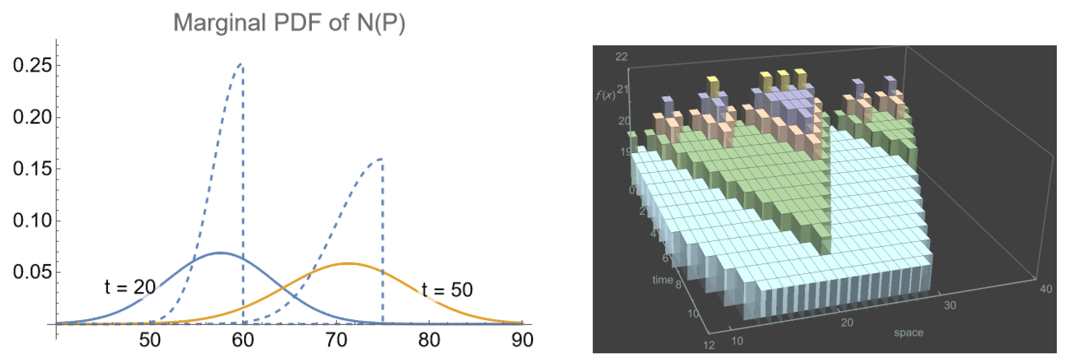
From the variational formulation (4) it becomes clear that the distribution of the vehicle number is given by the minimum of the Brownian motion over the finite interval . Conditional on the Brownian motion being zero at the beginning of the interval, , this minimum is known to have the half-normal distribution with parameter in our case. Since it follows that the probability density of conditional on is a shifted half-normal distribution given by:
with mean . A natural choice for would be :
and one can see that the stochastic solution is below the deterministic one, i.e. , as expected from Jensen’s inequality, but with the discrepancy increasing only as . The distribution (A1) is illustrated by the dashed lines in Figure A1.
The unconditional marginal distribution for is obtained by taking expectation of (A1) with respect to the distribution of , which is normal with mean and variance :
Unfortunately, analytical expressions for the moments of this distribution are unavailable at this time. Figure A1 (Left) illustrates the shape of this distribution at a fixed location and for different times. It can be seen that the distribution is much flatter than the half-normal distribution (A1) (dashed lines in the figure), as a consequence of large variance of .
A realization of the N-surface is shown in Figure A1 (Right), which depicts a 3D representation this surface in oblique coordinates where the third axis corresponds to deviations around the deterministic mean of the N-surface: . The random walk can be seen as a slice of this surface at , and the area under the random walk as the projection of the surface into the -plane; note that state C is lost in this projection.
Appendix B. Distribution of Local Flows and a Validation
A full description of the N-surface distribution, , has proven difficult to obtain, from which the distribution of flows, , could be derived. However, we have verified that the mean of the conditional (A1) and unconditional (A3) distributions are numerically very similar, and thus the mean flow can be approximated taking the time-derivative in (A2), to obtain:
where we have used instead of to emphasize that the flow is location-independent. Notice that this function starts at 0 at , increases rapidly to 0.4 by and flattens out to converge asymptotically to the capacity 1/2. (As a reference, recall that the critical headway is 2 time units.) That the flow is expected to be low at earlier times is a consequence of the system being farther from equilibrium at earlier times, which translates into an increased activity in jam interactions that produce little flow. As time goes by these interactions resolve to produce flows closer to capacity. This phenomenon can be seen in Figure 1, where it is clear that jam interactions are much more prevalent near the base of the triangle then near the bottom vertex.
Notice that the expected speed of traffic can be obtained simply by dividing (A4) by the critical density 1/2, which coincides with the finding in [41,49] obtained by approximating the dynamics of ECA 184. This is yet another statement of universality in traffic flow, where all the models mentioned in section 1, no matter discrete or continuum, describe the same phenomena.
To gain additional insights about the distribution of flows, note from Figure 1 that the flow can be either 1/2 in the capacity state or 0 in the void and congested states. Figure A2 shows the (oblique) cumulative counts and flow time series at 3 different locations for a typical rollout. The roughness of the cumulative curve is apparent as a result of the “spiky” variations in the flow around the capacity value 1/2. As a first approximation to describe the stochastic processes for flows, a fractional Gaussian noise process was fitted for 2000 realizations of flows timeseries. Also, a fractional Brownian motion process was estimated for the cumulative counts. Each panel shows the estimated Hurst exponent and the histograms summarize the results across rollouts. The average Hurst exponent for the flows is in line with the empirical results reported for Australian motorways (, [46]) and China’s highways (, [50]). This good agreement with empirical data gives a strong indication of the validity of the proposed framework.
Figure A2.
Oblique cumulative count and flow time series at 3 different locations for a typical rollout with . Notice that the flow time series have aggregated every 10 time steps for better visualization. Each panel shows the Hurst exponent estimated by fitting a fractional Brownian motion process for the cumulative counts and a fractional Gaussian noise process for the flows. The histograms summarizes the results for 2000 rollouts.
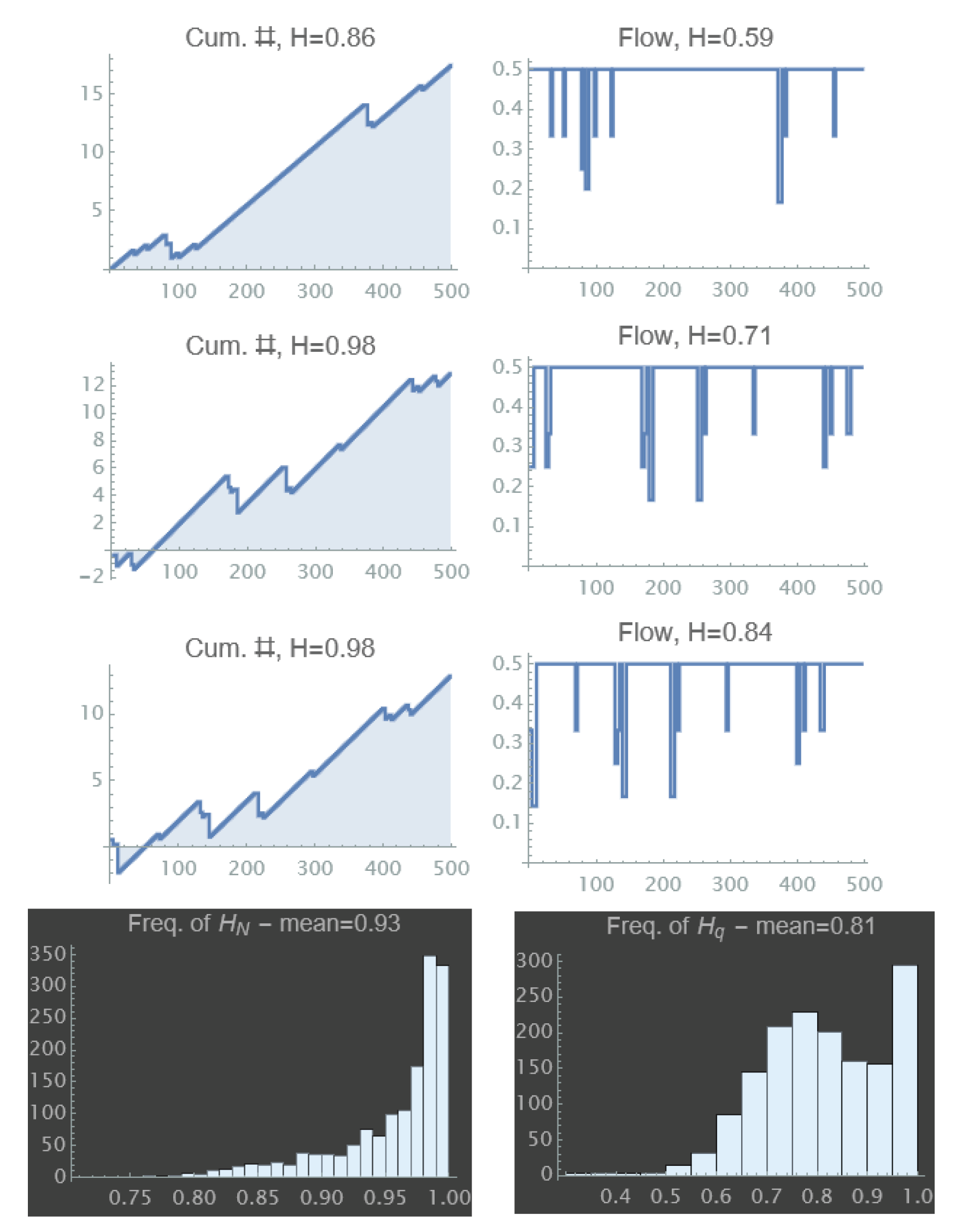
These high Hurst exponents indicate a long memory in the time series as a result of long-range spatial correlations. In this case these correlations are due to the spatial interactions brought about by the traffic model, which imposes long periods of constant capacity flow interrupted by bursts of null flow. Notice that the fractal dimension of the flow time series can be approximated by .
References
- Zeng, G.; Li, D.; Guo, S.; Gao, L.; Gao, Z.; Stanley, H.E.; Havlin, S. Switch between critical percolation modes in city traffic dynamics. Proceedings of the National Academy of Sciences 2019, 116, 23–28. [Google Scholar] [CrossRef] [PubMed]
- Zhang, L.; Zeng, G.; Li, D.; Huang, H.J.; Stanley, H.E.; Havlin, S. Scale-free resilience of real traffic jams. Proceedings of the National Academy of Sciences 2019, 116, 8673–8678. [Google Scholar] [CrossRef] [PubMed]
- Zeng, G.; Gao, J.; Shekhtman, L.; Guo, S.; Lv, W.; Wu, J.; Liu, H.; Levy, O.; Li, D.; Gao, Z.; others. Multiple metastable network states in urban traffic. Proceedings of the National Academy of Sciences 2020, 117, 17528–17534. [Google Scholar] [CrossRef] [PubMed]
- Bak, P.; Tang, C.; Wiesenfeld, K. Self-organized criticality: an explanation of 1/f noise. Phys. Rev. Lett 1987, 59, 381. [Google Scholar] [CrossRef]
- Dănilă, B.; Harko, T.; Mocanu, G. Self-organized criticality in a two-dimensional cellular automaton model of a magnetic flux tube with background flow. Monthly Notices of the Royal Astronomical Society 2015, 453, 2982–2991. [Google Scholar] [CrossRef]
- Aschwanden, M.J. A macroscopic description of a generalized self-organized criticality system: Astrophysical applications. The Astrophysical Journal 2014, 782, 54. [Google Scholar] [CrossRef]
- Nagatani, T. The physics of traffic jams. Reports on progress in physics 2002, 65, 1331. [Google Scholar] [CrossRef]
- Helbing, D. Traffic and related self-driven many-particle systems. Reviews of modern physics 2001, 73, 1067. [Google Scholar] [CrossRef]
- Chowdhury, D.; Santen, L.; Schadschneider, A. Statistical physics of vehicular traffic and some related systems. Physics Reports 2000, 329, 199–329. [Google Scholar] [CrossRef]
- Nagatani, T. Traffic flow on percolation-backbone fractal. Chaos, Solitons & Fractals 2020, 135, 109771. [Google Scholar]
- Taleb, N.N. Statistical consequences of fat tails: Real world preasymptotics, epistemology, and applications; STEM Academic Press, 2020. [Google Scholar]
- Halperin, B.; Hohenberg, P. Scaling laws for dynamic critical phenomena. Physical Review 1969, 177, 952. [Google Scholar] [CrossRef]
- Zipf, G. Human Behaviour and the Principle of Least Effort, 1949.
- Hurst, H.E. Long-term storage capacity of reservoirs. Transactions of the American society of civil engineers 1951, 116, 770–799. [Google Scholar] [CrossRef]
- Mori, T.; Smith, T.E.; Hsu, W.T. Common power laws for cities and spatial fractal structures. Proceedings of the National Academy of Sciences 2020, 117, 6469–6475. [Google Scholar] [CrossRef] [PubMed]
- West, G.B.; Brown, J.H.; Enquist, B.J. A general model for the origin of allometric scaling laws in biology. Science 1997, 276, 122–126. [Google Scholar] [CrossRef]
- Newman, M.E. Power laws, Pareto distributions and Zipf’s law. Contemporary physics 2005, 46, 323–351. [Google Scholar] [CrossRef]
- Mandelbrot, B.; Hudson, R.L. The Misbehavior of Markets: A fractal view of financial turbulence; Basic books, 2007. [Google Scholar]
- Kobayashi, Y.; Takayasu, H.; Havlin, S.; Takayasu, M. Robust Characterization of Multidimensional Scaling Relations between Size Measures for Business Firms. Entropy 2021, 23, 168. [Google Scholar] [CrossRef]
- Watanabe, H.; Takayasu, H.; Takayasu, M. Relations between allometric scalings and fluctuations in complex systems: The case of Japanese firms. Physica A: Statistical Mechanics and its Applications 2013, 392, 741–756. [Google Scholar] [CrossRef]
- Clauset, A.; Shalizi, C.R.; Newman, M.E. Power-law distributions in empirical data. SIAM review 2009, 51, 661–703. [Google Scholar] [CrossRef]
- Nagel, K.; Paczuski, M. Emergent traffic jams. Physical Review E 1995, 51, 2909. [Google Scholar] [CrossRef]
- Paczuski, M.; Nagel, K. Self-organized criticality and 1/f noise in traffic. Traffic and granular flow. World Scientific Singapore, 1996, p. 73.
- Nagel, K.; Schreckenberg, M. A cellular automaton model for freeway traffic. Journal de physique I 1992, 2, 2221–2229. [Google Scholar] [CrossRef]
- Daganzo, C.F. A Variational Formulation of Kinematic Wave Theory: basic theory and complex boundary conditions. Transportation Research Part B 2005, 39, 187–196. [Google Scholar] [CrossRef]
- Nagel, K. Personal communication, 2021.
- Schadschneider, A. Personal communication, 2021.
- Nagel, K.; Rasmussen, S.; Barrett, C.L. Network traffic as a self-organized critical phenomena. Technical report, Los Alamos National Lab., NM (United States), 1996.
- Rieser, M.; Nagel, K. Network breakdown “at the edge of chaos” in multi-agent traffic simulations. The European Physical Journal B 2008, 63, 321–327. [Google Scholar] [CrossRef]
- Olmos, L.E.; Çolak, S.; Shafiei, S.; Saberi, M.; González, M.C. Macroscopic dynamics and the collapse of urban traffic. Proceedings of the National Academy of Sciences 2018, 115, 12654–12661. [Google Scholar] [CrossRef] [PubMed]
- Lighthill, M.J.; Whitham, G.B. On kinematic waves II. A theory of traffic flow on long crowded roads. Proceedings of the Royal Society of London. Series A. Mathematical and Physical Sciences 1955, 229, 317–345. [Google Scholar]
- Richards, P.I. Shock waves on the highway. Operations research 1956, 4, 42–51. [Google Scholar] [CrossRef]
- Newell, G.F. A Simplified Car-Following Theory : a Lower Order Model. Transportation Research Part B 2002, 36, 195–205. [Google Scholar] [CrossRef]
- Daganzo, C.F. In Traffic Flow, Cellular Automata = Kinematic Waves. Transportation Research Part B 2006, 40, 396–403. [Google Scholar] [CrossRef]
- Laval, J.A.; Chilukuri, B.R. Symmetries in the kinematic wave model and a parameter-free representation of traffic flow. Transportation Research Part B: Methodological 2016, 89, 168–177. [Google Scholar] [CrossRef]
- Wolfram, S. Cellular automata as models of complexity. Nature 1984, 311, 419. [Google Scholar] [CrossRef]
- Laval, J.A.; Leclercq, L. The Hamilton-Jacobi partial differential equation and the three representations of traffic flow. Transportation Research Part B 2013, 52, 17–30. [Google Scholar] [CrossRef]
- Hopf, E. On the Right Weak Solution of the Cauchy Problem for a Quasilinear Equation of First Order. Indiana Univ. Math. J. 1970, 19, 483–487. [Google Scholar] [CrossRef]
- Schroeder, M. Fractals, chaos, power laws: Minutes from an infinite paradise; Courier Corporation, 2009.
- Zaliapin, I.; Kagan, Y.Y.; Schoenberg, F.P. Approximating the distribution of Pareto sums. Pure and Applied geophysics 2005, 162, 1187–1228. [Google Scholar] [CrossRef]
- Fuks, H. Solution of the density classification problem with two cellular automata rules. Physical Review E 1997, 55, R2081. [Google Scholar] [CrossRef]
- Edie, L.C. Discussion of Traffic Stream Measurements and Definitions. 2nd Int. Symp. on Transportation and Traffic Theory;, 1965; pp. 139–154.
- Majumdar, S.N.; Comtet, A. Airy distribution function: from the area under a Brownian excursion to the maximal height of fluctuating interfaces. Journal of Statistical Physics 2005, 119, 777–826. [Google Scholar] [CrossRef]
- Janson, S. Brownian excursion area, Wright’s constants in graph enumeration, and other Brownian areas. Probability Surveys 2007, 4, 80–145. [Google Scholar] [CrossRef]
- Agranov, T.; Zilber, P.; Smith, N.R.; Admon, T.; Roichman, Y.; Meerson, B. Airy distribution: Experiment, large deviations, and additional statistics. Physical Review Research 2020, 2, 013174. [Google Scholar] [CrossRef]
- Chand, S.; Aouad, G.; Dixit, V.V. Long-Range Dependence of Traffic Flow and Speed of a Motorway: Dynamics and Correlation with Historical Incidents. Transportation Research Record 2017, 2616, 49–57. [Google Scholar] [CrossRef]
- Krause, S.M.; Habel, L.; Guhr, T.; Schreckenberg, M. The importance of antipersistence for traffic jams. EPL (Europhysics Letters) 2017, 118, 38005. [Google Scholar] [CrossRef]
- Daganzo, C.F. The cell transmission model: A dynamic representation of highway traffic consistent with the hydrodynamic theory. Transportation Research Part B 1994, 28, 269–287. [Google Scholar] [CrossRef]
- Fuks, H.; Boccara, N. Generalized deterministic traffic rules. International journal of modern physics C 1998, 9, 1–12. [Google Scholar] [CrossRef]
- Shang, P.; Wan, M.; Kama, S. Fractal nature of highway traffic data. Computers & Mathematics with Applications 2007, 54, 107–116. [Google Scholar]
Figure 1.
Relationship between the random walk/excursion representing the fluctuations around the critical density in the initial conditions and the corresponding exact solution of the deterministic traffic flow model in the time-space diagram. The colored bars represent the congestion clusters or jams (traffic state J) in the time-space diagram, whose statistics are given by the return times of the random walk as shown. The dark gray bars are the voids (traffic state o) and the light gray areas the capacity state C. Notice that since these are the only traffic states possible, the total spatiotemporal area .
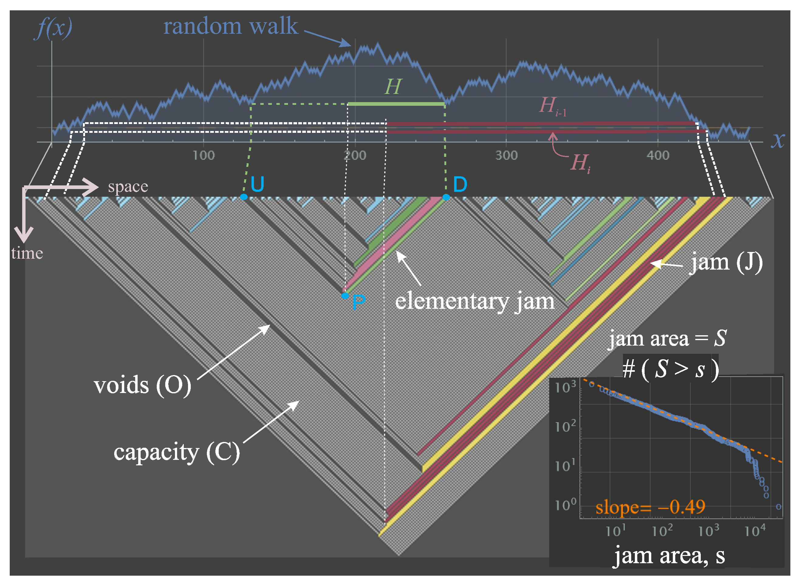
Figure 2.
Top: Estimated power-law exponent vs the initial density p for and ; orange regression lines and , respectively, estimated with data in . For lower values of the segment length results are similar but with a higher variance. Bottom: Detailed outputs for selected values of for .
Figure 2.
Top: Estimated power-law exponent vs the initial density p for and ; orange regression lines and , respectively, estimated with data in . For lower values of the segment length results are similar but with a higher variance. Bottom: Detailed outputs for selected values of for .
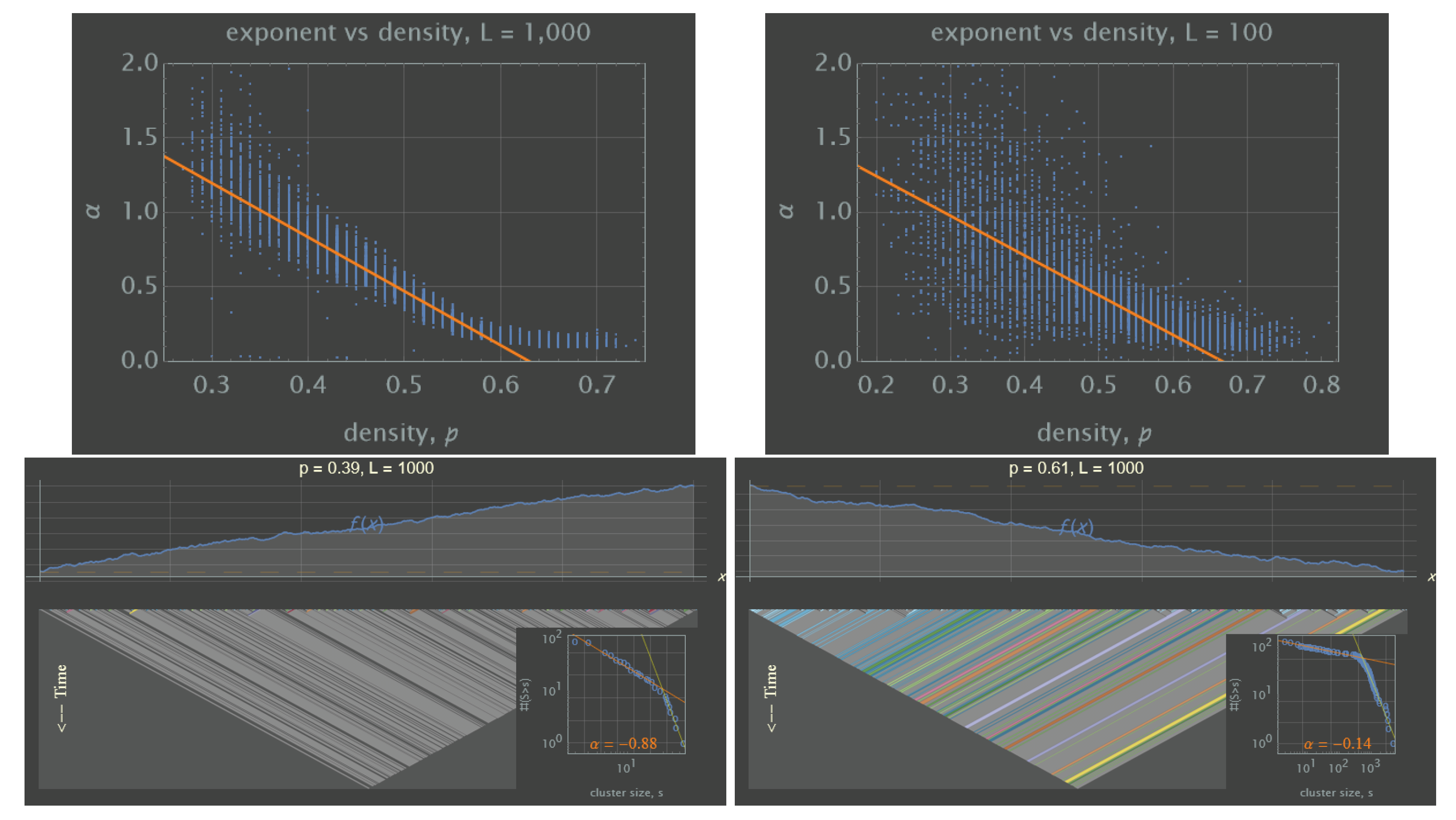
Figure 3.
PDF of the Airy distribution, , in blue. Although it is analytical, there is no closed-form expression for this distribution, only a complicated infinite sum [43], which is not implemented by default in most libraries/packages (the first 24 terms in this sum were considered for making this figure). The shaded area corresponds to the area under the Inverse Gaussian Distribution with mean parameter 0.625416 and shape parameter 9.82985, which can be seen to provide an accurate (and fast) approximation.
Disclaimer/Publisher’s Note: The statements, opinions and data contained in all publications are solely those of the individual author(s) and contributor(s) and not of MDPI and/or the editor(s). MDPI and/or the editor(s) disclaim responsibility for any injury to people or property resulting from any ideas, methods, instructions or products referred to in the content. |
© 2023 by the authors. Licensee MDPI, Basel, Switzerland. This article is an open access article distributed under the terms and conditions of the Creative Commons Attribution (CC BY) license (http://creativecommons.org/licenses/by/4.0/).
Copyright: This open access article is published under a Creative Commons CC BY 4.0 license, which permit the free download, distribution, and reuse, provided that the author and preprint are cited in any reuse.


