Submitted:
28 November 2025
Posted:
02 December 2025
You are already at the latest version
Abstract
An in-depth analysis of the drivers of agricultural emissions at the primary crop output and farm-gate levels is crucial to achieving net-zero emissions by 2050. This study examines the short- and long-run effects of crop production on farm-gate emissions in the regional trading bloc (RTB) member states in Africa. We proxy crop production by cereals, roots and tubers, vegetables, and fruits production, and split emissions into methane and nitrous oxide emissions. Furthermore, we collected data on these variables from 30 member states of the selected RTBs in Africa from 1990 to 2022, which we analyzed using the cross-sectional augmented autoregressive distributive lag approach that controls for endogeneity and heterogeneous slopes. We also employed the pooled mean group and sub-sample analyses as robustness checks to ensure the reliability of study findings. Our results revealed that cereal production increases farm-gate methane and nitrous oxide emissions in Africa’s RTB member states in the short and long run. The increase is between the range of 1.0021 to 1.0033 kilotons CO2–eq yr-1 for methane and 1.0024 to 1.0035 kilotons CO2–eq yr-1 for nitrous oxide on average. Thus, cereal production has a more adverse effect on nitrous oxide than methane emissions. In addition, fruit production increases farm gate methane emissions in Africa’s RTB member states by 1.0023 kiloton CO2–eq yr-1 on average in the long run. We recommend promoting climate-smart agriculture, investing in agricultural emissions monitoring, surveillance, and reporting systems, and targeting cereal and fruit production systems in RTB emission control plans.
Keywords:
STIRPAT
; methane
; nitrous oxides
; cereals
; fruits
; vegetables
; roots and tubers
1. Introduction
The global surface temperature rose by 1.1 Degree Celsius between 1850 and 1900 and between 2011 and 2020. Such a trend is expected to continue, partly with increases in greenhouse gas (GHG) emissions caused by human activities [1], posing a serious challenge in pegging warming to 1.5 degrees Celsius and achieving net zero emissions by 2050. These anthropogenic sources of GHG emissions include the Combustion of fossil fuels for energy generation, deforestation, and industrial operations [2], which contribute to climate change. Climate change causes drought, flooding, and heat stress. The combined effects of climate change, growing world population, and economic growth put significant pressure on the agricultural sector, particularly the crop subsector, to fulfill its roles [3,4,5].
Crops are the primary division of the agricultural sector. It can be categorized as the output from cereals, roots and tubers, vegetables, and fruits, which are geared towards increasing food security, reducing malnutrition, and increasing trade [6,7]. The achievement of the role of crops has become critical as crop production and animal numbers will need to increase by 60% from 2006 levels to meet the food demand for the 9.7 billion people in 2050 [8]. Approximately 80% of the desired increase in the food demand in developing nations is expected to be achieved through greater cropping intensity and yields, with the remaining 20% coming from the expansion of arable land [9].
Consequently, in Africa, the regional trading bloc (RTB) member states made commitments under the Malabo Declaration (MD) to accelerate growth in the agricultural sector, achieve food security, and improve livelihoods [10]. Tracking the progress made by RTBs in fulfilling the commitments of member states under the MD in 2022 revealed that the Southern African Development Community (SADC) experienced a 2.6 percentage rise in agricultural output from 2014 to 2022, the Economic Community of West African States (ECOWAS) recorded the highest percentage change in agricultural production of 3.2 percent followed by the East African Community (EAC) with a 2.7 percent increase. The lowest annual average (1.5 percent) was registered in the Arab Maghreb Union (AMU). For individual crops, such as maize and roots and tubers produced by the EAC, ECOWAS, and SADC in 2022, cassava, with the highest average for all crops, has significant growing potential across the RTBs. Cassava is the only non-cereal crop among the top five crops, and, along with yams, represents a huge proportion of agricultural output, thus underscoring the continent’s drive to attain food security [11].
The diversification of the agricultural sector in Africa extends beyond the provision of staples to trade. For instance, edible fruits and oil accounted for 21 percent of agricultural exports [11]. In addition, there is considerably higher variability in cereal production observed in RTB member states relative to the RTB level, suggesting the potential for intra-RTB trade [12]. However, the potential of the agricultural sector and trade to boost African economies is hindered by the effects of climate change.
The effect of climate change on the agricultural sector is far-reaching. The variability in climate alone is responsible for one-third of the agricultural variation [13]. The threat of climate change on traditional agrarian systems increases with the interaction of rising temperatures [14]. If adaptive measures are not taken to mitigate the effects of climate change, there is a possibility for a reduction in crop yield within the range of 7 and 23 percent and from 10 percent to 50 percent in 2030 [15]. A rise in specific methane (CH4) and nitrous oxide (N2O) emissions in the long run will further impact agricultural output [16]. The effects of climate change are more pronounced in Africa, where agriculture is predominantly rain-fed. Africa is susceptible to the impact of changing climates and bears disproportionate consequences, even though it contributes only 4 percent of the world's GHG emissions [17]. In Africa, maize, rice, wheat, groundnut, and vegetable yields are expected to decline by 3.4 percent, 6.9 percent, 11 percent, 9.1 percent, and 10.1 percent, respectively, in 2050 compared to the 2020 production level due to the effect of climate change [12].
Conversely, the agricultural sector is the second major contributor to GHG emissions. It contributes mainly to agricultural CH4 and N2O emissions [18]. The Agriculture, Forestry, and Other Land Use (AFOLU) total anthropogenic GHG emissions have grown on average from 13 percent to 21 percent between the periods 2010 and 2019. Deforestation accounts for 45 percent of agricultural emissions, partly due to land-use for agriculture, and agricultural CH4 and N2O emissions increased substantially from 2010 to 2019 [19]. Moreover, agriculture is a predominant emitter of farm gate emissions (FGEs) through the application of manure and nitrogen fertilizer [1], which contributes to climate change. Again, the contribution of CH4 from rice production to GHG emissions is approximately 96 percent [20], which exceeds the agricultural emissions from N2O [21]. This makes the agriculture sector the leading contributor to the rise in AFOLU, CH4, and N2O emissions [22].
Another factor that contributes to emissions is trade [2]. The proliferation of international trade agreements in the post-World War II era, in the form of multilateral, regional, or bilateral trade agreements, led to a surge in trade and economic growth [23,24,25].
The increase in trade volume followed by a proportionally greater increase in GHG emissions [26,27,28]. This is due to the increase in the standard of living and the rise in foreign demand, resulting in trade expansion and the extensive use of land, sea, air, and rail modes of transportation to take goods across different country borders. The movement of goods, especially to long-distance countries, involves large GHG emissions, which result in climate change [29]. The increase in world trade can deplete natural resources due to the rise in the volume of economic activities to meet the increasing foreign demand [30].
However, for countries with high population growth and biophysically less endowed, trade can be a useful means to import goods from countries with abundant water, land, and favorable climates suitable for the production of goods [31]. Trade can also play a role in cushioning the shortage of food supply due to crop failure, drought, and flooding by supplying the needed food through imports [32]. This minimizes the emissions of GHG from the importing country because there is less pressure on the environment to produce such goods [32].
The increase in trade will increase the GDP of the exporting countries. This rise in income will stimulate people's desire for better environmental quality and reduce GHG emissions [33]. Agricultural emissions can also be reduced through the technology impacts of trade and trade-related technology transfer. Among these technological spillover impacts of agrarian trade are the market competitiveness effect and the demonstration and imitation effect [34,35]. Agricultural carbon emissions can also be reduced by investing in energy-efficient technology and climate-smart agriculture, which is financed by the profit earned from the trade of farm products. This can encourage the advancement of industrial technology through technical support, technology licensing, and sales [36].
In conclusion, there is double-headed causality between crop production and emissions and between emissions and trade. Hence, these feedback effects between crop production and agricultural emissions, and trade and agricultural emissions, need to be investigated further to understand the drivers of crop-induced emissions at the RTB member states level and mitigate them. In this regard, a study from the Food and Agriculture Organization revealed that crop and livestock production are responsible for 10 to 12 percent of FGEs. In addition, 10 percent of these emissions is attributed to land use change [37].
In line with the interconnectedness of crop and livestock emissions, researchers have attempted to distinguish the contribution of crop production to emissions from livestock production, noting that carbon dioxide (CO2), N2O, and CH4 emissions occur at the various stages of the food production and consumption. In parallel, disaggregating food production emissions revealed that food crops contribute to N2O emissions. Furthermore, rice cultivation predominantly drives CH4 emissions, whereas CO2 emissions occur during the production of farm implements, farm operations, processing, and transportation [22].
A detailed review of the crop–emissions nexus revealed, for instance, in estimating the emission factor in China’s crop production, [38] showed that the average carbon footprint from crop production was 0.01-0.11 tons of CO2 equivalent per hectare per year. Zooming in on the various components that contribute to total emissions from crop production showed that emissions from the use of nitrogen fertilizer accounted for approximately 60 percent.
Using data on the major crops grown in China, [39] examined the direct and indirect contribution of crop production to emissions. Generally, they revealed that rice paddy contributed 0.37 kilograms of CO2 equivalent per kilogram of paddy rice output, which is approximately three times the contribution of wheat, maize, and soybean. Furthermore, considering the ecological environment, the study revealed that for dry land, the contribution of crops to N2O emissions (both direct and indirect) is 0.78 carbon footprint; for the lowland, direct CH4 emissions contributed 0.69. Globally, due to conventional flooding methods that produce anaerobic soil conditions, rice farming contributes 10-12 percent of methane emissions. The methane emissions figure may be understated, as according to [40], using satellite data, showed that for most rice-producing countries, methane intensities vary between 10 to 120 kg methane per ton of rice output, with a global average of 51.
Similarly, [41] studied the key contributing grain crops to carbon footprint to inform policies on the adoption of sustainable agricultural practices. They found that the carbon footprint of rice is the highest, followed by wheat and maize in that order. In addition, 341 grams of N2O emissions per hectare in a season caused by rice production [42].
In contrast, [43] assessed double rice production contribution to agricultural emissions in a bid to reduce carbon and nitrogen footprints and found out that, the CO2 equivalent emissions per kg of rice production in a year ranges from 0.83 to 0.85 for early, late, and double cropping, while N2O emissions from double cropping (10.68) is greater than early cropping (10.47), but less than late cropping (10.89).
To identify potential influencers of agricultural emissions and provide pathways to mitigate them, [44] used the Food and Agriculture Organization database and showed that maize production contributed the most to crop emissions (11.70 percent), followed by potatoes (10.21 percent) and rice (9.25 percent). In parallel, comparing mono-cropping and intercropping, [45] found that intercropping maize and potatoes immediately after nitrogen fertilization reduced N2O emissions by 19.0 percent–20.6 percent. Additionally, such a decrease is more noticeable in the short run.
Tracking the N2O emissions in an agricultural production greenhouse in the root zones of hydroponic tomato and cucumber plants on gravel-wool growth sacks with drip irrigation estimation using the static chamber method [46] revealed that the average emission factors for N2O were 0.13 percent for cucumber crop excluding drain re-use (open hydroponic method) and 0.31 percent for the cultivation of tomatoes with drain recycling (closed hydroponic technology). Furthermore, measuring and comprehending the shifting patterns of smallholder agricultural systems' soil N2O emissions in Sub-Saharan Africa [47] revealed that, among other variables, vegetables emit 48 to 113.4 kg N2O-N ha-1 yr−1.
According to [48], the production and trade of vegetables and fruits across borders negatively impact the environment. However, 16 percent of such emissions can be mitigated by optimizing nitrogen fertilizer usage [49].
We can deduce from reviewing relevant past studies that crop production contributes directly to CH4 and N2O emissions, though the contribution to nitrous oxide emissions is more pronounced, while contributing indirectly to CO2 in these study areas. Again, despite the role played by the agricultural sector and trade in explaining emissions, amidst, the growing pressure on the crop subsector to achieve food security in the presence of climate change effects, a study that specifically examine the short-and long-term effects of individual crops, such as cereals, roots and tubers, vegetables, and fruits, which are most susceptible to climate change [50] at the farm-gate level on CH4 and N2O emissions, in the RTB member states are scarce. This study, as a novelty, investigates the short- and long-run effects of crop production on farm-gate emissions in the regional trading bloc member states in Africa. To achieve this objective, we proxy crop production by cereals, roots and tubers, vegetables, and fruits production and split emissions into CH4 and N2O as the dominant emissions components at the farm-gate level. Furthermore, we collected data on these variables from 30 member states of the major RTBs in Africa from 1990 to 2022, which we analyzed using the cross-sectional augmented autoregressive distributive lag approach that controls for endogeneity and heterogeneous slopes. We also employed the pooled mean group and sub-sample analyses as robustness checks to ensure the reliability of study findings.
This study makes three contributions to air quality. First, our study is perhaps among the few that focus on the primary root cause of agricultural emissions by zooming into the different sub-components of the crop sector, such as cereals, roots and tubers, and fruits, and linking them to the predominant (CH4 and N2O) emissions components at the farm gate level. The second contribution of our study is that it employs the panel autoregressive distributive lag (ARDL) method, which controls for cross-sectional dependency, structural breaks, slope heterogeneity, serial correlation, and endogeneity. It also accounts for the long-run effects of crop production on agricultural emissions. This enhances the robustness and reliability of our regression findings.
Thirdly, considering the role played by trade in promoting and mitigating emissions, the analysis of the crop production and emissions nexus at the RTB level member states level provides insights into the different crops that are notorious emitters of CH4 and N2O emissions, and suggests pathways to mitigate them at the RTB member states and RTB levels.
Thus, with the introduction of carbon financing, the imposition of taxes on dirty goods at the international trade level, and the coordination of the activities of the RTBs in Africa, this study is important, as it exposes specific crops that are notorious emitters of GHGs. Using this information, the various blocs will be empowered to design a coordinated approach to minimizing emissions and to determine the amount of money producers of dirty goods can be charged by Environmentalists at the RTB member states' level.
2. Materials and Methods
2.1. Crop Production and Farm-Gate Level Emissions Framework
Crop production involves several processes referred to as value chains. The crop value chains comprise the assembling of inputs such as fertilizer, pesticides, and tools (Downstream production activities). Land preparation, tillage, irrigation, and other activities before the product leaves the farm (Primary production activities), and harvesting, threshing, processing, storage, and transport to market (Upstream production activities). Thus, emitting CO2, CH4, and N2O in the process (Figure 1).
From panel A in Figure 1, the manufacturing of fertilizer and pesticides, the production and packaging of seeds, and the transportation of farm inputs to assemble inputs for crop production contribute mainly to CO2 emissions [22]. Moreover, in India, crop production accounts for 87 percent of emissions from food production [22]. The carbon footprint from crop production activities, such as tillage and irrigation (panel B), is associated with CH4 and N2O emissions. For instance, for dry cover crop, soil deficit irrigation decreases N2O relative to full irrigation [51]. Furthermore, no-tillage reduces N2O relative to tillage [52]. Again, rice cultivation increases CH4 emissions, while food crops contribute to N2O [22]. Panel C comprises highly mechanized activities that are prone to CO2 emissions. Upstream activities such as harvesting, threshing, processing, and transportation increase the use of fossil fuels. The further shift from small-scale to large-scale farming increases energy use, energy intensity, and dependence on fossil fuels, which promotes CO2 emissions [53,54].
From the Figure 1 and the review of the literature, we observed that CH4 and N2O are the major contributors to the carbon footprint from direct crop production, occurring at the farm-gate level (panel B). Thus, an effective crop emission mitigation strategy should target emissions at the farm-gate level where crop-based emissions are predominant. Hence, this study's main focus is on CH4 and N2O emissions at the farm-gate level.
2.2. Regression Strategy
We estimate our regression models using the strategy in Figure 2. A common mistake researchers make in panel model specification is to specify a static model instead of a dynamic model. When a model is misspecified, there is a good chance that the estimated residuals from the regression equation will exhibit some autocorrelation [55]. Thus, we specify a dynamic model because we believe that past emissions are associated with current emissions. Consequently, in our estimation strategy, we first conduct a cross-sectional dependence (CD) test using the [56] tests to examine the strength of CD, with the null hypothesis of weak CD. In the presence of CD, we conduct the second-generation unit root test because it is robust in dealing with CD [57]. We use the Pesaran cross-augmented Dickey-Fuller (Pescadf) test based on the individual Dickey-Fuller or augmented Dickey-Fuller means [58].
With large cross-section and time dimensions, we use the standardized version of Swamey's test to test for slope heterogeneity, because the incorrect imposition of slope heterogeneity will result in biased and inconsistent results [59]. Furthermore, the prevalence of policy shifts or shocks in macroeconomics warrants a structural breaks test as its omission will lead to misleading inferences. In the presence of CD, slope heterogeneity, and structural breaks, we employ the cross-sectional augmented autoregressive distributive lag (CS-ARDL) model that controls for these problems. We interpret the estimated coefficients obtained from the regressions using proportional changes. We also conduct robustness checks to validate our results, using the pooled mean group (PMG) estimation technique and sub-sample analysis. We use Stata 17 [60] to conduct all empirical estimations.
2.3. Theoretical Specification of the Regression Model
Researchers have developed several models of climate change human drivers. Typical of such theories is the environmental impact of population, affluence, and technology (IPAT). This theory, by [61], shows that population (P), affluence (A), and technology (T) are the drivers of environmental degradation. The IPAT provides the foundation for several other climate change theories, such as the STIRPAT. The STIRPAT, developed by [62], improves on the IPAT by incorporating a stochastic term and non-unit elasticity of the environmental impact of each driving force. Since our study examines the effects of crop production on FGEs by running a regression, we adopt the STIRPAT model to illustrate the stochastic relationship between crop production on FGEs, as shown by [63]. The theoretical specification of the STIRPAT is depicted in the following equation:
Taking the natural logarithm throughout yields:
where are the coefficients to be estimated, , natural logarithm, and is the error term assumed to be normally distributed.
2.4. Empirical Model Specification
[64] employed the STIRPAT model to study emissions in economies at various stages of development. For instance, [65] proxied environmental degradation with CO2 and N2O emissions, while [66] proxied affluence with crop and livestock production indices. Several other proxies have been proposed for population and technological driving forces of emissions. Hence, we use N2O and CH4 emissions indicators for FGEs because they are the two most prevalent emission components in the agricultural sector [41]. Additionally, to explicitly distinguish the contribution of the crop sector's primary output to emissions at the farm gate level, we proxy affluence into cereals, roots and tubers, vegetables, and fruit production. This is because they are the crops that are commonly grown in the member states for which data is available and they contribute significantly to the gross domestic product (GDP) of these member states.
We employ agricultural investment (Tech) and rural population (Rupop) as proxies for technology and population, respectively, and observe them as control variables. Thus, we specify a dynamic augmented STIRPAT panel model to investigate the relationship between crop production and FGEs in selected African RTB member states as follows:
where represent member states, , years, and, previous year.
2.5. Method of Estimation
2.5.1. Diagnostic Tests
2.5.1.1. Cross-Sectional Dependence Test
We are motivated to apply the CD because these RTB member states are interconnected in the sense that they share common languages, cultures, and traditions. In addition, they belong to the same blocs, hence there is the likelihood that they share similar trade policies, and with globalization, participate in regional or global value chains. Thus, to test for CD in the panel data set, we employ the [56] test for weak CD. We use this test because it can be applied to balanced [56] and unbalanced panels [67], and is more robust in detecting CD in large time and cross-sectional units [56]. The null hypothesis is weak CD.
where is the correlation between the sample residuals, is a reliable predictor of the variance.
2.5.1.2. Second-Generation Unit Root Test
With the assumption of CD, the [58] test for stationarity is used to determine the unit root of the variables because of its simplicity. The Pesaran unit root test is predicated on the statistical significance of specific cross-sectionally augmented Dickey-Fuller test statistics. Additionally, it modified the Im Pesaran Shin t-bar test statistic to test for stationarity when the residuals are correlated and CD is present. Hence, the name cross-sectional specific augmented Im Pesaran Shin (CIPS). The null hypothesis of the CIPS is that there is no unit root.
where N is the number of cross-sectional units, and represents units.
2.5.1.3. Test for Slope Homogeneity
With the assumption of stationarity of the variables, we test for slope homogeneity across the panel units using the [59] test for homogeneous slope because it is more applicable for larger panels. Under the null hypothesis of slope homogeneity, Pesaran and Yamagata estimated two test statistics as illustrated in (2.7 and 2.8):
where is the pooled ordinary least squares estimator of the slope coefficients, is the weighted fixed effect of the slope coefficients, the identity matrix is given as , and the estimator of is . The standardize dispersion statistic ()is given as:
where is Swamy test statistic, N is the number of cross-sectional units, and is the degree of freedom.
2.5.1.4. Test for Structural Breaks
Structural breaks may be prevalent, particularly in macroeconomic data, due to policy shifts or shocks. These changes, whether known or unknown, may affect the interpretation of regression results and inferences. As such, [68] proposed a model to detect multiple breaks in panel data. The panel data model, consisting of a structural break k, is written as:
for
where is the endogenous variable and and are exogenous variables. are vectors of coefficients. means error term and represent the structural break dates.
The error term allowed unobserved heterogeneity through the specification of an interactive fixed effects shown as:
Where is the unobserved common factor, is the factor loading, the idiosyncratic error is , and the interactive effect is
The is likely to be correlated with the exogenous variables. To capture this, we specify the exogenous variables:
whereand are factor loadings. The idiosyncratic errors are and . captures the correlation of the independent variables within and across cross-sections.
2.6. Cross-Sectionally Augmented Autoregressive Distributed Lag
Assuming our model is dynamic with a mixed order of integration, autocorrelation, endogeneity, long-run relationship, heterogeneous slopes, and structural breaks, we are open to three dynamic common correlation effect estimation methods: cross-sectional augmented distributed lag (CS-DL), the CS-ARDL, and the error-correction model augmented autoregressive distributed lag (ECM-ARDL) models. However, in our study, we use the CS-ARDL model to overcome the limitation of the CS-DL; it does not estimate the error correction term (ECT) that accounts for the speed of adjustment in the long-run equilibrium. Also, the CS-ARDL and the ECM-ARDL are similar long-run estimation techniques, as they account for ECT and produce numerically equivalent regression output [67]. We specify the CS-ARDL model as:
where (nitrous oxide and methane emissions) is the endogenous variable, is the constant, is the speed of adjustment; which shows the speed at which the emissions converge to long run equilibrium after a short run shock such as the COVID, and the commitment to pegging emissions, is the vector of the slope parameters of the exogenous variables, and lagged endogenous variables. is a vector of the independent variables and are the long-run unobserved factors and are the short-run unobserved factors.
2.7. Proportional change coefficients
Since equations (2.3) and (2.4) are written in natural log, we interpret the regression coefficients using elasticity. However, our dependent variables (farm gate methane and nitrous oxide emissions) are reported yearly [30]. Hence, it is required that we convert the emissions elasticity to proportional change coefficients of emissions with the help of the preceding formula [31]:
where represents exponent, , The predicted regression coefficient (α) represents the predicted rise in emissions, the change's size is denoted by m.
2.8. Data
We sampled the RTB member states because crop production plays a significant role in their growth. Figure 3 shows that RTB member states selected for our study have a greater contribution of crop production to GDP, as indicated by the closeness of crop production values to GDP on the far left end of the horizontal line. However, a few member states, like South Africa, Côte d'Ivoire, and Nigeria, have values closer to the right, probably because they have more robust extractive, industrial, or service sectors, which raise GDP above crop production. Notwithstanding, crop production still has a role to play in these RTB member states if we net out the contribution of the extractive industries, especially oil and precious minerals such as diamond and gold, as Africa generally, is characterized as an agrarian economy.
Furthermore, some of these member states belong to more than one RTB due to overlapping membership. For instance, the United Republic of Tanzania, which belongs to RTBs such as the SADC, and EAC. In addition, there are also RTBs whose membership extends beyond regional boundaries, like the Common Market for East and Southern Africa (COMESA). Therefore, it is difficult to study these member states and RTBs. To unpack the complexity, we exclude the RTBs with a deeper cross-regional geographical scope. As such, we drop RTBs like COMESA. Thus, we select the AMU, EAC, ECOWAS, and SADC RTBs in the north, east, west, and southern regions, respectively. These four RTBs selected comprise forty-four (44) member states: five (5) from AMU, eight (8) from EAC, fifteen (15) from ECOWAS, and sixteen (16) from SADC. In addition, we exclude member states with overlapping membership to avoid duplication (Tanzania), giving us a total of forty-two (42) member states. We then exclude twelve (12) member states based on data availability on common crops produced: Cereals, vegetables, roots and tubers, and fruits, and rural population, and technology. Thus, our final sample consists of thirty (30) member states, which represent approximately 70 percent of the RTB member states (see Table 1).
2.9. Selection of key variables
Carbon dioxide equivalent emissions can broadly reflect emissions from crops, livestock, and forestry divisions. However, for a detailed analysis, we focus on the crop sub-sector’s contribution to emissions. This is because crop production faces increased pressure due to the rising world population and the attainment of food security; crop emission intensity becomes critical, as it may be associated with higher emissions. In this regard, crop emissions can result from upstream, downstream, and farm-gate levels. However, the predominant CO2 equivalent emissions at the farm-gate level, which account for the direct contribution of crops to emissions, are methane and nitrous oxide emissions [18], as revealed by studies such as [39,40,45,49]. Thus, we employ methane and nitrous oxide emissions as our dependent variables.
Crops have faced increased pressure due to the population's growing demand for food, which requires crop intensity and yield to increase by 80 percent [8,9]. The increase in cropping intensity and yield arguably will increase agricultural emissions. The 10 major crops grown in Africa are maize, sorghum, cassava, millet, rice, groundnuts, cowpeas, wheat, beans, and vegetables. The production of these crops is expected to increase from 36.5 percent to 127.6 percent, with a corresponding increase in emissions from 0.5 to 5.2 percent from 2020 to 2050 [12]. Thus, by categorizing these crops into different food groups, such as cereals, roots and tubers, vegetables and fruits, we can quantify crop contribution to emissions as of 2022 and use the results to proffer measures to reduce emissions below the projected 5.2 percent in 2050. In addition, we include fruit production to capture its contribution to emissions to account for how the African continent’s drive to achieve nutrition security actually impacts emissions. Extant studies have examined the contribution of fruits [48,49], vegetables [46,47], roots and tubers [43,45], and cereal crops [39,42] to emissions, respectively. The control variables, such as population and technology, have also been employed by authors such as [71,72] to determine their effect on emissions. As such, we use these variables as independent variables in our study to determine their effect on CH4 and N2O emissions at the farm-gate level in the RTBs member states in Africa. We collected data on the variables for the sampled RTB member states from the Food and Agriculture Organization Statistical database [73] from 1990 to 2022. The description of the variable is presented in Table 2.
2.10. Trend Analyses
From Figure 4, given that roots and tubers are comparatively stationary, member states of the AMU bloc, including Algeria, Morocco, Tunisia, and Mauritania, show stable, slight growth paths for fruits and cereals. The Mediterranean environment and irrigation-driven practices that support crop choice and yield stability in the AMU are apparent in this trend. The absence of notable shifts in root and tuber in agricultural production shows that root and tuber are not significantly impacting climate change, nor are they a priority. Focusing on the EAC, countries like Kenya, Uganda, Tanzania, Rwanda, and Burundi continue to grow a variety of crops, with cereals, vegetables, roots and tubers, and fruits demonstrating an increasing trend. This regional dependence on numerous farming techniques and the adaptability of its agricultural policies have been emphasized by this smooth, comprehensive growth [74]. The general upward trend indicates adaptable agricultural practices and efficient production; however, fluctuations in cereal and fruit production show vulnerabilities to year-to-year climatic conditions. Nigeria, Ghana, Côte d'Ivoire, Benin, Burkina Faso, Mali, and Senegal are ECOWAS member states with substantial increases in cereals, roots, and tubers. The important role crops play in ensuring household food security reflects such patterns. However, the trends show that several ECOWAS member states, notably Ghana and Nigeria, experience frequent shocks, which may be attributed to changes in input prices, significant climate variability, and shifting governmental policies [75]. Furthermore, there has not been an enormous spike in fruits and vegetables, implying that although the cultivation of vegetables is frequently done on a smaller scale, it capitalizes on controlled environments that protect against changes in the climate, such as irrigation systems [76]. South Africa, Angola, Mozambique, Namibia, Madagascar, Mauritius, and Lesotho constitute the member states that collectively make up the SADC bloc in this study. The predominant trend in this bloc is resilience, especially in terms of cereal output, which aligns with Southern Africa's greater extent of agricultural modernization and state support. Nevertheless, they lag behind cereals in growth trends. Fruits, vegetables, roots, and tubers also show a continuing positive trend, suggesting continuing progress in both the primary food and growing crop sectors. Although climate or structural shocks are undoubtedly the cause of the sporadic variability in member states like Madagascar and Lesotho, SADC member states often strive to sustain consistent trends over the years [77,78].
2.11. Growth in Methane and Nitrous Oxide Emissions
Over the past three decades, CH4 and N2O emissions have grown steadily and modestly throughout member states of the AMU, including Algeria, Morocco, and Tunisia. Large irrigation and more mechanized agriculture systems are perhaps all contributors to this resilience, with minimal variation for either GHG, the emissions patterns in AMU countries point to persistent progress in input handling and possibly more uniform implementation of environmental regulations [79]. A slightly distinct perspective is given by the EAC, which includes Kenya, Uganda, Tanzania, Rwanda, and Burundi. In this bloc, CH4 and N2O emission trends show slight consistent increases, especially in Kenya and Tanzania. These trends underscore the region's diverse and intensive farming methods. Importantly, weaker agricultural sectors or more reliance on small-scale farming may account for Burundi and Rwanda's reduced emission rates [80]. These patterns highlight how crucial crop management and extension services are in determining the scale and variability of GHG rise throughout EAC in the long run. The emissions narrative is more volatile in the ECOWAS. The magnitude and intensity of the agricultural sector shifted, access to agricultural inputs fluctuated, and large-scale climatic changes have contributed to the sporadic rises and falls in member states like Ghana and Nigeria. Smaller member states like Benin, Sierra Leone, and Togo, contrarily, indicate consistent but slower rises. The significant influence of environmental pollution on emission trends across ECOWAS member states shows the importance of policy coordination across crop management and climate adaptation options [81]. Notwithstanding notable differences between the region's more productive and less productive economies, the SADC bloc represents the African perspective. South Africa stands apart in that its emission trajectory is completely flat and consistent, which indicates its innovative rules and regulations and mechanized agricultural practices [82,83]. CH4 and N2O emissions shift marginally in other SADC member states, such as Mozambique, Namibia, Madagascar, and Lesotho. This is likely linked to fluctuations in rainfall and the interaction between subsistence and commercial farming (see Figure 5).
2.12. Crop Methane and Nitrous Oxide Intensity
Crop CH4 and N2O intensities across the RTBs in Africa depict several trends and patterns. Consequently, CH4 and N2O emission intensities remain low and stable for most member states' crops in this study. Remarkably, fruits and vegetables generally have the lowest emission intensities associated with upland and low-intensive farming practices for crop cultivation. There are occasionally notable fluctuations in emission intensity despite the general predictability; these are mostly linked to roots and tubers, and, to a lesser extent, cereals. Lesotho, Madagascar, Liberia, Mozambique, and Senegal are noteworthy examples of these unexpected rises in CH4 and N2O emissions per unit of output, which are mainly from member states and seasonal in source. The rises are likely triggered by several interconnected factors, such as productivity volatility, variations in farming practices, sporadic climate variations, and shifts toward more wetland or waterlogged cultivation techniques, especially for cereals [84]. In addition, CH4 intensity appears to be more volatile than N2O. This may be due to its greater susceptibility to aerobic conditions prevalent in waterlogged rice and tuber fields [85].
By analyzing specific crop shifts, CH4 intensity for cereals typically remains low but often jumps drastically in member states with intermittent fluctuations in land use or farming techniques. Similarly, temporal stability is observed in N2O intensity for cereals, with only a few minor fluctuations. This may indicate that fertilizer management is mostly efficient across a large number of member states, with exceptional inconsistencies. Roots and tubers are especially vulnerable to unexpected fluctuations in CH4 and N2O intensities. This phenomenon can frequently be attributed to shifts in the application of organic material, floodplain cultivation, or yield variability triggered by global warming. Fruits and vegetables, on the other hand, appear to be among the most stable and climate-resilient crops; their relatively low and predictable structures result from cultivation techniques that promote efficient nutrient utilization and reduce the creation of adverse microorganisms [86,87]. Notably, fruit crops provide low-intensity production methods with low GHG emissions. These results imply that management and policy interventions aimed at limiting input-based emission spikes in cereals, roots, and tubers, as well as facilitating a rise in fruit and vegetable farming, can offer effective routes leading to environmentally friendly cultivation in the RTB member states in Africa [88] (see Figure 6).
3. Results
3.1. Descriptive Analyzes
Table 3 shows that, on average, the regional trading bloc member states emitted 38.62 kilotons of CH4 and 2.81 kilotons of N2O. The key drivers of these emissions are crop production, the size of the rural population, and expenditure on technology. However, the ECOWAS and AMU member states stood out as the major regional trading blocs whose member states are driving these emissions. That is, while the ECOWAS member states are the major emitter of CH4 emissions (574.89 kilotons), the AMU member states are the principal emitter of N2O (42.13 kilotons). The dominance in farm-gate emissions by the AMU and ECOWAS member states can be attributed to the ECOWAS member states engaging in large scale cereal farming with little or no emissions mitigation practices, as such, produces the highest cereals (48.1 million metric tons), and roots and tubers (123 million metric tons), and having the largest average rural population (167 million people) engaging in unfriendly environmental agricultural activities such as the burning of crop residues [18]. Furthermore, the AMU member states produce the highest vegetables (25.7 million metric tons) and fruits (32.1 million metric tons), which are high-emitting crops that drive the intensity of fertilizer usage (technology). This further explains why the AMU member states spend the most on technology (US$201.35 billion) [89].
Moreover, an analysis of the individual indicators reveals that the lower similar differences in means between the SADC and the EAC member states in terms of fruit, and vegetable production suggest that these regional trading bloc member states share similar agro-ecological conditions, farming practices, and agricultural policies. However, there are differences in mean for cereal production across the regional trading bloc member states, with the ECOWAS member states having the highest positive mean difference. This signifies variation in terms of the scale of farming, the type of crops cultivated, and the intensity of fertilizer usage. The ECOWAS member states are ahead of other regional trading bloc member states in terms of the scale of farming and fertilizer application, among other factors. There is also a large variation in the rural population across the regional trading bloc member states in Africa, with the ECOWAS member states noting the highest positive value. The variance of the variables symbolizes the disparity in farm-gate CH4 and N2O emissions and their drivers across the regional trading bloc member states.
3.2. Diagnostic Tests
First, in our regression approach, we test for the existence of CD. We employ the [56] test to determine the correlation between the RTB member states because it is suitable for unbalanced panels and more robust than the [90] CD test. The null hypothesis in this test is a weak CD between the RTB member states. From Table 4, the probability values of the variables in the CH4 and N2O models are statistically significant at the 1% level. Hence, we reject the null hypothesis of a weak CD and confirm the existence of a strong CD across the panels in both equations.
Since there is a CD, we conduct a second-generation unit root test. We use the [58] second-generation unit root test and Z[t-bar], which is based on the average of the particular Dickey-Fuller (or Augmented Dickey-Fuller) t-statistics from each panel unit for constant term and constant term and trend in level and first difference. According to the null hypothesis, every variable is non-stationary. From Table 5 and Table 6, the variables are stationary at the level for the "constant" and "constant and trend." However, roots and tubers, and technological variables are non-stationary at the level of the “constant.” Similarly, technology also has a unit root at the level of the "constant and trend." Conclusively, there is mixed integration of order one and zero. However, all variables are integrated to order one for both "constant" and "constant and trend" in the CH4 and N2O models.
Furthermore, we perform a test for slope heterogeneity. The test null hypothesis is that the slope coefficients are uniform. The coefficients are statistically significant at the 1% level, rejecting the null hypothesis and declaring the presence of heterogeneous slopes among the panels (Table 7).
For the CH4 emissions model, Table 8 shows that for the one versus no structural breaks, two versus one structural break, and three versus two structural break hypotheses tested, the t-statistic is below the critical values at 1%, 5%, and 10% levels of statistical significance. Thus, we fail to reject the null hypotheses and conclude that there is a stable trend in the data structure. Similarly, data on the N2O emissions for the first break [F(1/0)] does not detect any statistically significant shift in the data structure. However, the data structure strongly supports the second and third breaks over their respective lags. Thus, over time, there are significant breaks in the N2O data in 1999, 2006, and 2015. These breaks may be associated with the credit crunch in 2007 and the commitment made by member states to reduce emissions in 2015.
From the diagnostic tests, we confirmed the presence of CD, structural/no structural breaks, and heterogeneous slope coefficients in equations (2.3) and (2.4). Hence, we use the CS-ARDL model to address these issues jointly.
3.3. Crop Production and Farm Gate Emissions: Short and Long-Run Relationships
The study examines the short-and long-run effects of crop production on farm-gate emissions in selected RTB member states in Africa. We achieve this objective by proxying crop production to mean cereals, roots and tubers, vegetable, and fruit production and separate emissions into methane and nitrous oxide emissions. We employ the CS-ARDL model, which is dynamic, controls for CD, slope heterogeneity, serial correlation, structural breaks, and endogeneity [61] to estimate our baseline model (2.13).
3.3.1. Crop Production and Methane Emissions: Short and Long Run Relationships
Table 9 shows that all crop products have a positive sign, except roots and tubers. This means that roots and tubers are the only products with the potential to reduce methane emissions at the farm gate level in the RTB member states. However, cereals and fruit products are the crop products that affect methane emissions in the short and long run. The lag of methane emissions is also significant, validating the specification of a dynamic model. Analytically, cereals have short-run proportional change coefficients of 1.0021 and 1.0033 for the long term. This means that an increase in cereal output will result in a 1.0021 and 1.0033 kilotons on CO2 equivalent emissions increase in farm-gate methane emissions in the short and long run on average in a year, respectively. Thus, the production of cereals is a significant contributor to farm-gate emissions. Its contribution increases by 0.0012 kilotons of CO2 equivalent emissions, yearly, in the long run. Likewise, fruit production makes a positive contribution to farm-gate methane emissions in the RTB member states in Africa, both in the short and long run. Fruit production has a short-run proportional change coefficient of 1.0019 and a long-run proportional change coefficient of 1.0023. This indicates that fruit production significantly increases farm gate methane emissions in both the short and long term. Additionally, the increase in farm-gate methane emissions caused by fruit production is exacerbated in the long run by 0.004 kilotons of CO2 equivalent emissions on average, yearly. This implies that fruit production is a significant contributor to farm-gate methane emissions. The lag of emissions has a co-efficient of 0.8664. The lag of the emissions coefficient shows that past emissions are correlated with present emissions, hence the estimated model is dynamic. Further-more, the negative error correction term [ECM (-1)] with a speed of adjustment of 0.866 confirms the presence of a long-run relationship, implying that approximately 87% of disequilibrium in emissions is corrected annually through policies geared towards reducing methane emissions and negative shocks. The F-statistic has a coefficient of 2.78, which means that the model is well-fitted.
3.3.2. Crop Production and Nitrous Oxide Emissions: Short and Long-Run Relationships
Cereals and the production of fruit have a positive influence on the emissions of nitrous oxide in the short term. However, cereals are the sole contributors that may account for nitrous oxide emissions in the long term (Table 10). The positive signs on the coefficients of cereals and fruits show that they are the crops that drive farm-gate nitrous oxide emissions in the member states of the regional trading blocs in Africa. Specifically, an increase in cereal production will result in a 1.0024 and 1.0035 kilotons of CO2 equivalent emissions increase in nitrous oxide on average in a year in the short and long run, respectively. Table 10 also shows that fruit production has a proportional change coefficient of 1.0025. Thus, a move to increase fruit production by a percentage point will result in a 1.0025 kiloton of CO2 equivalent emissions rise in nitrous oxide on average in a year in the short run. The error correction term is -0.8422. This depicts a long-run relationship and an 84.22 percent disequilibrium adjustment of nitrous oxide emissions after a shock every year. Moreover, the lag of the emissions coefficient is 0.1578 and statistically significant at 1% level. This implies that previous years’ emissions explain present emissions, hence confirming the use of a dynamic model. The F-statistic coefficient is statistically significant, representing the overall goodness of fit of the nitrous oxide regression model.
3.4. Robustness Checks: Pooled Mean Group and Sub-Sample Analysis
We use the PMG and subsample techniques to validate our baseline model results.
3.4.1. Pooled Mean Group Results
The PMG estimator was proposed by [92]. It is a dynamic model that permits group differences in short-run coefficients and error variances while constraining long-run coefficients to be the same. This estimation technique is robust because cross-sectional units can be pooled and also averaged. Table 11 shows the results of the PMG model. The results suggest that the cereals variable has a positive sign in the short and long run for the methane and nitrous oxide emissions models. These results confirmed the findings presented in Table 9. In addition, the positive fruit production effect on methane emissions is also confirmed in the long run (Table 9). However, vegetables, the rural population, and technology also have long-run effects on methane emissions.
3.4.2. Sub-Sample Results
Our sample comprises member states in the four selected regional trading blocs in Africa: The AMU, the EAC, the ECOWAS, and the SADC. The largest regional trading bloc in the sample is the SADC in terms of membership. Therefore, using the same estimation technique (CS-ARDL model), we estimate the sub-sample of the SADC regional trading bloc member states. We compare the regional trading bloc member states sub-sample findings to the full sample to corroborate the CS-ARDL results for all the regional trading bloc member states in this study. The results reveal that both the short and long-run effects of cereals on farm-gate emissions for methane and nitrous oxide, as well as the long-term effect of fruit production on farm-gate emissions for methane, are statistically significant at 1% level (Table 13 and Table 14).
This confirms that cereals and fruit production are the drivers of methane and nitrous oxide emissions (Table 9 and Table 10).
Conclusively, all the models confirm that cereals and fruit production are the drivers of methane and nitrous oxide emissions at different periods, and the existence of a long-run relationship between the variables, with a speed of adjustment ranging from 39% to 86% for every diversion of the emissions variable due to shocks.
4. Discussion
Attaining net zero emissions by 2050 requires a reduction in the emission of greenhouse gases. However, results from the cross-sectionally augmented autoregressive distributive lag estimation technique, pooled mean group method, and the sub-sample analyses consistently show that cereal and fruit production drive farm-gate methane and nitrous oxide emissions in the regional trading bloc member states in Africa. Cereals are notorious emitters of both methane and nitrous oxide emissions in the short- and long-run. However, the effect of cereals on nitrous oxide emissions is more pronounced than on methane emissions. This result is not striking because the increase in area under cereal cultivation and application of fertilizer are strongly associated with rises in nitrous oxide emissions across the regional trading bloc's member states. On the contrary, agricultural activities such as rice cultivation or occasionally flooded crop fields cause less significant methane emissions. [93,94] supported these findings by demonstrating that agriculture-related nitrous oxide emissions are strongly driven by cereal cultivation and fertilizer use, even though methane emissions tend to be more closely linked with cereals through shifts in land use or organic management.
Specifically, from Table 9, a standard deviation increase in cereal production will result in a rise in farm-gate methane emissions of 1.0021 and 1.0033 kilotons of CO2 equivalent year-1 on average in the short- and long-run, respectively. Thus, suggesting that the continuous cultivation of cereals in waterlogged farmlands, the production of agricultural byproducts such as rice straw, incomplete combustion of burnt remnants, and the burning of crop residues may be significant contributors to methane emissions in Africa’s regional trading bloc member states. The positive long-run relationship may also imply that the focus of RTB member states is to increase cereal output rather than engage in farm-gate methane emissions mitigation strategies, such as climate-smart agriculture, due to lack of training, technological challenges, and high startup costs, which leads to long-term growth in farm-gate methane emissions [95,96]. This finding aligns with [39,40], which suggested that crop production contributes directly to methane emissions through the use of conventional flooding methods. This finding is also consistent with the results of [95,97,98], which showed that increasing grain production leads to increased agricultural emissions due to the expensive coupling interruption of decoupling activities and the adoption of inefficient agricultural practices.
Similarly, cereals also drive nitrous oxide emissions in the regional trading bloc members’ states. This is because of their significant positive proportional change value. Hence, a move by regional trading bloc member states to increase cereal production by a standard deviation will lead to a 1.0024 and 1.0035 kilotons of CO2 equivalent yr-1 on average rise in farm-gate nitrous oxide emissions in the short- and long-run, respectively. The increase in nitrous oxide emissions may be a result of farmers' adoption of tillage and conventional irrigation, which disturb soil structure and increase microbiological channels for generating nitrous oxide [99]. The impact of cereal on nitrous oxide emissions may also be surmountable when cereal cultivation is done on a predominantly unsustainable basis [100]. The result supports the findings of [40,41,42], which revealed that cereals such as rice, wheat, and maize in mixed order are significant drivers of nitrous oxide emissions in mono-cropping, intercropping, early, late, and double cropping. Furthermore, this study finding aligns with [101], who stated that differences in temperature requirements for crops grown accounted for the accumulation of more nitrous oxide emissions by cereals compared to legumes. However, [102] finding suggested that nitrous oxide emissions were reduced through the correct selection of cereal varieties and sustainable agricultural practices.
In addition to cereals, fruit production is identified as a long-run driver of methane emissions. It has a positive long-run proportional change coefficient, indicating that higher fruit output results in a 1.0023 kilotons of CO2 equivalent increase in farm-gate methane emissions on average per year. This is likely because fruit cultivation involves land-use changes, tillage, irrigation, mulching, or manure application, all of which can disrupt soil and raise methane emissions [103]. In addition, land use change for unsustainable agricultural production may increase the incidence of methane emissions over time [104]. [48,105] study result confirmed that fruit production can deplete water resources as a result of shifting demand for crops that require adequate water, such as avocado. In summary, cereals drive both methane and nitrous oxide emissions over time, while fruits mainly affect methane emissions. Policymakers in agriculture, climate, and trade should consider these relationships when developing strategies to increase output, promote trade, and mitigate these emissions.
5. Conclusions
The drivers of crop emissions are diverse, so limiting them to crop output will be generic and, as such, will not provide a significant contribution to the crop emissions literature, therefore, this study employs the STIRPAT model, which considers multiple drivers of emissions and is more appropriate in determining causal short- and long-run effects of crop production on farm-gate emissions in the regional trading blocs member states in Africa. This study focuses primarily on the root causes of agricultural emissions by zooming into the different sub-components of the crop sector, such as cereals, roots and tubers, and fruits, and linking them to emissions (methane and nitrous oxide) at the farm-gate level. Furthermore, we employ the CS-ARDL technique that is robust and ensures the reliability of our study findings. Our results revealed that cereal production increases farm-gate methane and nitrous oxide emissions in Africa’s regional trading bloc member states in the short- and long-run. The increase is between the range of 1.0021 to 1.0033 kilotons for methane, and 1.0024 to 1.0035 kilotons for nitrous oxide emissions per year. Thus, cereal production has a more adverse effect on nitrous oxide than methane emissions. In addition, fruit production increases farm gate methane emissions in Africa’s regional trading bloc member states by 1.0023 kiloton per year on average in the long run.
We offer the following policy suggestions in light of our empirical findings. First, regional agricultural policies should incentivize the uptake of climate-smart agriculture adoption technologies and practices such as low or minimum tillage, alternative wetting and drying, and the conversion of crop residues into biochar. Second, member states and regional trading blocs should invest in agricultural emissions monitoring, surveillance, and reporting systems to track and mitigate real-time farm gate-level emissions from the different primary crops. Third, we recommend the targeting of cereal and fruit production systems specifically, through the adoption of good agricultural practices such as crop residue management and improved irrigation systems. These should be included in farm-gate emissions mitigation plans.
Notwithstanding, this study has limitations. Notably, since the crop sub-sector is a fraction of the agricultural sector, other sub-sectors like livestock and forestry that also have the potential to drive farm-gate emissions should be studied for a comprehensive analysis of farm-gate emissions in the agricultural sector. However, they are excluded because the focus of this study is to provide a detailed investigation that is manageable, robust, and free from too much of complexities. Thus, this study lays the foundation for future research in the livestock and forestry sub-sectors. Again, aside from farm-gate emissions, we have pre- and post-crop production emissions, which we do not account for; hence, it also serves as a potential area for future research.
Author Contributions
Conceptualization, L.S., and J.M., methodology, L.S., IPP.,and J.M., analysis and interpretation L.S., J.M., I.P-P., and A.M.M.; writing—review and editing, J.M., I.P-P., and A.M.M.; supervision, J.M., I.P-P., and A.M.M. All authors have read and agreed to the published version of the manuscript.
Funding
This research received no external funding.
Institutional Review Board Statement
Not applicable.
Informed Consent Statement
Not applicable.
Data Availability Statement
Data on supporting reported results can be found on the Food and Agriculture Organization Statistics (FAOSTAT) database through the link: https://www.fao.org/faostat/en/#data/QCL.
Conflicts of Interest
The authors declare no conflict of interest.
Appendix A
Appendix A.1

Appendix 1.
Showing summary statistics for member states.
| RTB | Methane | Nitrous Oxide |
Cereals | Roots & Tubers | Vegetables | Fruits | Population | Technology |
|---|---|---|---|---|---|---|---|---|
| Algeria | 1.905452 | 2.195615 | 3379664 | 2607641 | 3903938 | 3739872 | 12040.52 | 908.7052 |
| 0.438419 | 0.6875611 | 1406411 | 1593811 | 2139947 | 2097809 | 487.5547 | 785.5285 | |
| 0.9479 | 1.0524 | 870017 | 715936 | 1300588 | 1242788 | 11247.75 | -584.325 | |
| 2.876 | 3.4472 | 6066239 | 5020249 | 7986966 | 7071434 | 12718.63 | 2584.071 | |
| 33 | 33 | 33 | 33 | 33 | 33 | 33 | 33 | |
| Angola | 7.192694 | 0.7512727 | 1218094 | 8470025 | 1008288 | 2349265 | 9078.947 | 28557.11 |
| 3.490819 | 0.5161117 | 969838.1 | 4782581 | 638038.5 | 2089799 | 1123.496 | 29812.68 | |
| 2.6818 | 0.2208 | 248500 | 1798899 | 250000 | 405000 | 7650.444 | -334.5 | |
| 13.0039 | 1.739 | 3179113 | 1.83E+07 | 2016573 | 6120250 | 11168.04 | 106077 | |
| 33 | 33 | 33 | 33 | 33 | 33 | 33 | 33 | |
| Benin | 3.604391 | 0.7639091 | 1307770 | 5107649 | 398597.7 | 348965.8 | 4840.86 | 1254.186 |
| 1.950024 | 0.5667518 | 559093.4 | 1890488 | 181999.4 | 169602.2 | 971.806 | 1113.204 | |
| 1.4687 | 0.3029 | 545898 | 2019754 | 214645 | 173161.4 | 3261.667 | 40.58002 | |
| 7.7358 | 2.2982 | 2320756 | 7952286 | 744746.3 | 676228.8 | 6450.295 | 3840.753 | |
| 33 | 33 | 33 | 33 | 33 | 33 | 33 | 33 | |
| Burkina Faso | 24.57023 | 1.640588 | 3551293 | 130609.8 | 702582.7 | 537292.6 | 11015.93 | 1800.319 |
| 16.64094 | 0.6425372 | 1081092 | 72103.9 | 387412.5 | 467407.7 | 2256.687 | 1809.728 | |
| 5.0237 | 0.745 | 1517900 | 37400 | 229116 | 69831 | 7593.826 | 0.466252 | |
| 58.7137 | 2.6971 | 5180702 | 299127 | 1416382 | 1429305 | 15056.71 | 6551.879 | |
| 33 | 33 | 33 | 33 | 33 | 33 | 33 | 33 | |
| Burundi | 2.325809 | 0.2462879 | 384242.2 | 2198305 | 348509.8 | 1592571 | 7330.446 | 364.0649 |
| 1.223799 | 0.1261564 | 278550.4 | 1070159 | 115611.1 | 312135.2 | 1799.806 | 319.3043 | |
| 1.0551 | 0.148 | 224724 | 1262722 | 210000 | 957109.6 | 5075.806 | 1.25543 | |
| 5.0285 | 0.5487 | 1581835 | 4419890 | 498160.5 | 2355697 | 10848.08 | 1493.657 | |
| 33 | 33 | 33 | 33 | 33 | 33 | 33 | 33 | |
| Cabo Verde | 0.085012 | 0.0075242 | 7812.303 | 13383.7 | 29258.79 | 14251.07 | 195.4066 | 434.141 |
| 0.010498 | 0.0023795 | 7383.527 | 4118.413 | 14497.6 | 2805.704 | 5.275204 | 577.4965 | |
| 0.043 | 0.003 | 4 | 7665 | 4682 | 6998.93 | 188.641 | 0.2526 | |
| 0.0952 | 0.0139 | 36439 | 21263 | 49973.16 | 19007 | 202.818 | 1619.846 | |
| 33 | 33 | 33 | 33 | 33 | 33 | 33 | 33 | |
| Côte d'Ivoire | 18.02668 | 1.277182 | 1898790 | 8439046 | 659303.4 | 2317163 | 10262.68 | 3502.637 |
| 5.700347 | 0.4033769 | 809132.4 | 3082855 | 60097.09 | 369014.7 | 1580.021 | 2029.808 | |
| 11.6375 | 0.6558 | 1221428 | 4685380 | 569753.7 | 1569720 | 7440.947 | 51.42595 | |
| 28.4025 | 2.1361 | 3308600 | 1.48E+07 | 774260.6 | 3155808 | 13017.21 | 8534.646 | |
| 33 | 33 | 33 | 33 | 33 | 33 | 33 | 33 | |
| Egypt | 165.8874 | 27.34557 | 2.01E+07 | 3760665 | 1.36E+07 | 1.11E+07 | 45550.75 | 111816 |
| 23.36905 | 4.536444 | 3288880 | 1745015 | 3373522 | 3181650 | 8533.03 | 71348.61 | |
| 105.1472 | 18.1261 | 1.30E+07 | 1600411 | 7459974 | 5977551 | 32450.63 | 735.7677 | |
| 213.8234 | 32.8514 | 2.41E+07 | 7712031 | 1.88E+07 | 1.60E+07 | 60691.93 | 237047.7 | |
| 33 | 33 | 33 | 33 | 33 | 33 | 33 | 33 | |
| Eswatini | 0.277246 | 0.1351758 | 92247.19 | 61337.73 | 11885.88 | 125597.1 | 891.9663 | 67.35088 |
| 0.040951 | 0.043385 | 28131.74 | 12613.61 | 941.323 | 24748.44 | 129.0743 | 54.09466 | |
| 0.1934 | 0.06 | 27540.66 | 43917 | 10500 | 73787.1 | 687.362 | -61.24678 | |
| 0.3672 | 0.2055 | 152068 | 94364.16 | 13345.9 | 162715.6 | 1121.095 | 154.906 | |
| 33 | 33 | 33 | 33 | 33 | 33 | 33 | 33 | |
| Ghana | 13.51608 | 1.243152 | 2440180 | 1.91E+07 | 628941.7 | 3804305 | 11441.48 | 5472.179 |
| 5.778714 | 0.7866342 | 1063430 | 8996124 | 141073.7 | 1767052 | 1242.964 | 5165.18 | |
| 4.6275 | 0.4273 | 843800 | 4409038 | 376972 | 923900 | 9297.561 | 17.8893 | |
| 27.9498 | 2.8538 | 5136565 | 3.82E+07 | 801831.5 | 6397830 | 13250.62 | 12706.64 | |
| 33 | 33 | 33 | 33 | 33 | 33 | 33 | 33 | |
| Guinea | 117.139 | 0.8987758 | 2525157 | 1644864 | 523224 | 1157566 | 6757.862 | 191.5825 |
| 60.07551 | 0.4303149 | 1084393 | 904542 | 35209.19 | 188701.8 | 1262.806 | 344.631 | |
| 48.791 | 0.3627 | 1061616 | 797775 | 440139 | 856803 | 4348.022 | -101.0378 | |
| 210.1131 | 1.699 | 4745053 | 4313086 | 566956.1 | 1614579 | 9022.706 | 1606.981 | |
| 33 | 33 | 33 | 33 | 33 | 33 | 33 | 33 | |
| Kenya | 6.481606 | 2.968221 | 3571863 | 2877909 | 1959503 | 2652795 | 29252.15 | 13663.48 |
| 1.450239 | 1.049515 | 725022.5 | 1035765 | 600950.9 | 863644.3 | 6204.769 | 13785.9 | |
| 4.6951 | 1.6589 | 2539301 | 1437978 | 743080 | 1400923 | 19483.07 | 72.99437 | |
| 8.7265 | 5.5514 | 4881251 | 4734181 | 3359488 | 4468921 | 39817.14 | 54593.73 | |
| 33 | 33 | 33 | 33 | 33 | 33 | 33 | 33 | |
| Lesotho | 0.338167 | 0.076803 | 127164 | 96997.26 | 27664.9 | 16010.38 | 1528.87 | 332.808 |
| 0.102067 | 0.0336183 | 64141.44 | 26693.76 | 5322.99 | 1412.726 | 73.75202 | 329.0402 | |
| 0.0889 | 0.0439 | 25678.06 | 45093 | 18000 | 13000 | 1379.922 | -0.808339 | |
| 0.5059 | 0.189 | 257418 | 134962.1 | 35000 | 19000 | 1667.714 | 1234.286 | |
| 33 | 33 | 33 | 33 | 33 | 33 | 33 | 33 | |
| Liberia | 2.361979 | 0.1458152 | 202201.8 | 524923.6 | 95278.76 | 173197.3 | 1786.776 | 19926.22 |
| 0.942721 | 0.0820897 | 85830.44 | 144054.1 | 19784.49 | 33465.9 | 515.1272 | 27234.66 | |
| 0.6364 | 0.0284 | 50000 | 232616.2 | 70996 | 106779 | 865.312 | 34.98093 | |
| 4.1834 | 0.2741 | 335180 | 769796.3 | 125356.5 | 217563 | 2517.04 | 83520.52 | |
| 33 | 33 | 33 | 33 | 33 | 33 | 33 | 33 | |
| Madagascar | 226.4066 | 1.324564 | 3647026 | 3899903 | 394242 | 1031850 | 13197.81 | 368.2073 |
| 27.27257 | 0.2881333 | 914651.2 | 630112.1 | 51151.28 | 188307.3 | 2698.242 | 365.3614 | |
| 181.7254 | 0.9841 | 2497184 | 2960139 | 330300 | 767800 | 8865.351 | 9.493062 | |
| 299.3309 | 1.8974 | 5159721 | 5183376 | 470948.3 | 1289990 | 17539.78 | 1349.597 | |
| 33 | 33 | 33 | 33 | 33 | 33 | 33 | 33 | |
| Mali | 38.44375 | 2.425688 | 5033452 | 453662.6 | 1234188 | 1116921 | 8967.909 | 1584.893 |
| 17.99707 | 1.435104 | 3010112 | 380888.9 | 555779 | 729994 | 1622.212 | 1750.402 | |
| 14.5249 | 0.7811 | 1771419 | 51296 | 296290 | 392951 | 6490.895 | 5.72972 | |
| 72.7271 | 5.8646 | 1.05E+07 | 1452527 | 2597052 | 2576204 | 11739.44 | 7679.898 | |
| 33 | 33 | 33 | 33 | 33 | 33 | 33 | 33 | |
| Mauritius | 0.119464 | 0.2005242 | 797.1212 | 17387.83 | 70759.96 | 18964.32 | 698.8862 | 1992.217 |
| 0.022647 | 0.050414 | 609.1133 | 3161.57 | 12109.77 | 6331.794 | 50.06979 | 1680.117 | |
| 0.069 | 0.1103 | 112 | 11654 | 44860.04 | 8370 | 592.342 | 14.77845 | |
| 0.1627 | 0.2829 | 2284 | 23317 | 93811.71 | 31958 | 756.756 | 4496.445 | |
| 33 | 33 | 33 | 33 | 33 | 33 | 33 | 33 | |
| Morocco | 5.501603 | 6.341245 | 6476768 | 1452429 | 3434894 | 4305758 | 13440.26 | 60297.24 |
| 0.767112 | 1.375903 | 2974395 | 353152.4 | 847129.7 | 1277107 | 264.3674 | 40605.3 | |
| 3.3945 | 3.6116 | 1783230 | 894210.1 | 1907077 | 2337928 | 12839.86 | 183.6424 | |
| 7.2056 | 9.3447 | 1.17E+07 | 1967534 | 4491362 | 6618471 | 13688.17 | 126623 | |
| 33 | 33 | 33 | 33 | 33 | 33 | 33 | 33 | |
| Mozambique | 21.15526 | 1.0946 | 1610493 | 5582967 | 529814.5 | 565793.1 | 15181.41 | 3954.453 |
| 7.960271 | 0.5334569 | 613783.8 | 1269572 | 553516.3 | 253428.9 | 3433.196 | 3487.002 | |
| 9.8411 | 0.357 | 244554.1 | 3365024 | 115282 | 280400 | 9935.737 | 23.39897 | |
| 33.6098 | 2.1766 | 2832309 | 7482694 | 2224968 | 1019695 | 21121.58 | 10952.81 | |
| 33 | 33 | 33 | 33 | 33 | 33 | 33 | 33 | |
| Namibia | 0.078303 | 0.1339364 | 114871.4 | 306863.5 | 39039.43 | 37611.89 | 1244.316 | 4406.658 |
| 0.019693 | 0.1550612 | 34827.81 | 66667.26 | 22936.58 | 20785.69 | 77.46508 | 3499.005 | |
| 0.0492 | 0.0161 | 31031 | 195000 | 8000 | 7998.06 | 1023.439 | 29.56727 | |
| 0.128 | 0.6772 | 186008.3 | 392075.9 | 67982.48 | 71123.62 | 1299.607 | 13785.07 | |
| 33 | 33 | 33 | 33 | 33 | 33 | 33 | 33 | |
| Niger | 2.366433 | 1.502612 | 3778998 | 331297.2 | 1250303 | 336543.6 | 12683.56 | 1130.317 |
| 0.592847 | 0.45282 | 1416583 | 278992.1 | 1050195 | 243196.4 | 4475.574 | 1183.053 | |
| 1.4677 | 0.8449 | 1850285 | 118320 | 249554.9 | 43800 | 6781.413 | 40.8132 | |
| 3.6941 | 2.2857 | 6100262 | 1103733 | 3605640 | 762360.2 | 21584 | 4599.48 | |
| 33 | 33 | 33 | 33 | 33 | 33 | 33 | 33 | |
| Nigeria | 306.2426 | 11.53765 | 2.40E+07 | 8.35E+07 | 1.07E+07 | 1.02E+07 | 85076.73 | 48374.03 |
| 108.4399 | 3.369717 | 3808570 | 2.88E+07 | 3836856 | 2359821 | 10149.39 | 47687.52 | |
| 147.9306 | 8.0291 | 1.77E+07 | 3.36E+07 | 4168000 | 6382000 | 66993.86 | 1002.5 | |
| 524.1397 | 21.0704 | 3.03E+07 | 1.36E+08 | 1.64E+07 | 1.69E+07 | 100786.3 | 150428.2 | |
| 33 | 33 | 33 | 33 | 33 | 33 | 33 | 33 | |
| Rwanda | 1.519518 | 0.3443 | 461602.6 | 2758519 | 412058.7 | 2672650 | 7985.937 | 1548.135 |
| 1.032416 | 0.1874906 | 244435.2 | 1037497 | 216855.7 | 438034 | 1786.131 | 2075.845 | |
| 0.1871 | 0.0635 | 130072.5 | 886071.8 | 121412.9 | 1549000 | 5344.914 | 7.66 | |
| 3.1715 | 0.7487 | 932107.3 | 4485985 | 688418.3 | 3611200 | 11247.44 | 7046.425 | |
| 33 | 33 | 33 | 33 | 33 | 33 | 33 | 33 | |
| Senegal | 11.22151 | 0.7853939 | 1593330 | 441460.1 | 436945 | 586966.3 | 6801.549 | 3171.29 |
| 7.981554 | 0.4486956 | 861180 | 506957.2 | 323109.5 | 516698.2 | 1390.933 | 2647.756 | |
| 3.405 | 0.2624 | 730335 | 41762.52 | 69661 | 167637 | 4616.787 | 57.85107 | |
| 29.6551 | 1.9716 | 3663690 | 1688559 | 1048198 | 1997619 | 9231.74 | 10463.86 | |
| 33 | 33 | 33 | 33 | 33 | 33 | 33 | 33 | |
| Sierra Leone | 35.25101 | 0.4251121 | 831425.9 | 1703635 | 279722.5 | 214152.9 | 3617.961 | 170.6266 |
| 14.89276 | 0.2197511 | 431829.1 | 1342271 | 87725.94 | 48840.27 | 680.6779 | 228.7765 | |
| 12.3042 | 0.1111 | 222472 | 224400 | 180000 | 152985 | 2797.796 | -7.46292 | |
| 78.3878 | 0.9433 | 2131723 | 4038764 | 479186 | 282814.1 | 4704.509 | 968.7065 | |
| 33 | 33 | 33 | 33 | 33 | 33 | 33 | 33 | |
| South Africa | 10.38005 | 11.81278 | 1.33E+07 | 1974537 | 2303409 | 5821977 | 19334.56 | 73580.81 |
| 2.08042 | 1.795304 | 3257667 | 459713.8 | 294933.3 | 1346182 | 439.1242 | 59399.63 | |
| 7.2043 | 9.2471 | 5056342 | 1125028 | 1892468 | 3815637 | 18015.16 | -78.45956 | |
| 14.6091 | 17.0976 | 1.96E+07 | 2763924 | 2724794 | 8772836 | 19800.02 | 182594.3 | |
| 33 | 33 | 33 | 33 | 33 | 33 | 33 | 33 | |
| Togo | 2.061203 | 0.4702273 | 946571.4 | 1514481 | 144587.5 | 55243.69 | 3778.373 | 919.5698 |
| 0.761084 | 0.1918064 | 307205 | 390027.1 | 5667.2 | 9354.613 | 696.5604 | 948.4203 | |
| 0.9135 | 0.2865 | 464877 | 840495.5 | 130698.4 | 41660.19 | 2704.301 | 22.72051 | |
| 3.329 | 1.0891 | 1439850 | 2244231 | 158700 | 68459.46 | 4927.839 | 3053.119 | |
| 33 | 33 | 33 | 33 | 33 | 33 | 33 | 33 | |
| Tunisia | 0.799524 | 1.928185 | 1725829 | 337181.8 | 2092994 | 1679399 | 3548.361 | 20842.69 |
| 0.232564 | 0.4039127 | 592995.9 | 76908.41 | 729207.2 | 442289.3 | 48.18436 | 10423.03 | |
| 0.3224 | 1.0384 | 550525.5 | 199000 | 1096862 | 1049565 | 3462.236 | 101.8172 | |
| 1.3492 | 2.9206 | 2896345 | 465000 | 3219344 | 2530206 | 3622.883 | 43107.63 | |
| 33 | 33 | 33 | 33 | 33 | 33 | 33 | 33 | |
| Uganda | 8.826661 | 0.9874939 | 2809803 | 5777216 | 884843.6 | 7835354 | 25121.42 | 2800.509 |
| 4.010887 | 0.2932797 | 942322.6 | 1671836 | 382722.5 | 2448102 | 6620.009 | 2786.402 | |
| 3.9167 | 0.5389 | 1576000 | 3501000 | 415500 | 3451798 | 15507.4 | -5.624783 | |
| 21.7561 | 1.8818 | 5525000 | 8765000 | 1412799 | 1.18E+07 | 37099.64 | 8707.827 | |
| 33 | 33 | 33 | 33 | 33 | 33 | 33 | 33 | |
| United Republic | 124.485 | 3.347121 | 6959240 | 8634589 | 1806026 | 3652592 | 30820.69 | 4679.756 |
| 54.25941 | 1.67222 | 3043055 | 2112238 | 736986.4 | 1737320 | 6471.257 | 4708.991 | |
| 53.3253 | 1.4451 | 2952900 | 4862263 | 1013675 | 1213738 | 20651.76 | 5.606912 | |
| 226.4278 | 7.1964 | 1.25E+07 | 1.32E+07 | 3182946 | 5884175 | 42177.77 | 19276.83 | |
| 33 | 33 | 33 | 33 | 33 | 33 | 33 | 33 | |
| Total | 38.61901 | 2.811911 | 3801119 | 5788327 | 1663200 | 2338144 | 13449.15 | 13937.07 |
| 77.89167 | 5.535796 | 5813586 | 1.60E+07 | 3175679 | 3150028 | 17080.64 | 33767.77 | |
| 0.043 | 0.003 | 4 | 7665 | 4682 | 6998.93 | 188.641 | -584.325 | |
| 524.1397 | 32.8514 | 3.03E+07 | 1.36E+08 | 1.88E+07 | 1.69E+07 | 100786.3 | 237047.7 | |
| 990 | 990 | 990 | 990 | 990 | 990 | 990 | 990 |
References
- IPCC. [1] IPCC. 2023. Summary for Policymakers: Synthesis Report. Climate Change 2023: Synthesis Report. Contribution of Working Groups I, II and III to the Sixth Assessment Report of the Intergovernmental Panel on Climate Change, studies, Pp: 1–34.
- Rafiq, S.; Salim, R.; Apergis, N. Agriculture, trade openness and emissions: an empirical analysis and policy options. Aust. J. Agric. Resour. Econ. 2016, 60, 348–365. [Google Scholar] [CrossRef]
- Hamad, A.A.A.; Ni, L.; Shaghaleh, H.; Elsadek, E.; Hamoud, Y.A. Effect of Carbon Content in Wheat Straw Biochar on N2O and CO2 Emissions and Pakchoi Productivity Under Different Soil Moisture Conditions. Sustainability 2023, 15, 5100. [Google Scholar] [CrossRef]
- Kotz, M.; Levermann, A.; Wenz, L. The effect of rainfall changes on economic production. Nature 2022, 601, 223–227. [Google Scholar] [CrossRef]
- Chaudhry, S.; Sidhu, G.P.S. Climate change regulated abiotic stress mechanisms in plants: a comprehensive review. Plant Cell Rep. 2022, 41, 1–31. [Google Scholar] [CrossRef] [PubMed]
- Varma, V.; Mosedale, J.R.; Alvarez, J.A.G.; Bebber, D.P. Socio-economic factors constrain climate change adaptation in a tropical export crop. Nat. Food 2025, 6, 343–352. [Google Scholar] [CrossRef]
- Kaur, N.; Kaur, S.; Agarwal, A.; Sabharwal, M.; Tripathi, A.D. Amaranthus crop for food security and sustainable food systems. Planta 2024, 260, 1–17. [Google Scholar] [CrossRef]
- United Nations Department of Economic and Social Affairs, Population Division 2022. World Population Prospects 2022: Summary of Results. UN DESA/POP/2022/TR/NO. 3.
- Eise, J.; Foster, K.A. (Eds.) How to Feed the World; Island Press: Washington, DC, USA, 2018. [Google Scholar] [CrossRef]
- African Union, 2014. Available online: https://www.resakss.org/node/ 6454?region=aw/retrieve (accessed on 23 August 2025).
- Statista 2025. Agriculture in Africa - statistics and facts. Available online: https://www.statista.com/topics/12901/agriculture-in-africa/#topicOverview (accessed on 28 September 2025).
- Tadesse, B.; Ahmed, M. Impact of adoption of climate smart agricultural practices to minimize production risk in Ethiopia: A systematic review. J. Agric. Food Res. 2023, 13. [Google Scholar] [CrossRef]
- Howden, S.M.; Soussana, J.-F.; Tubiello, F.N.; Chhetri, N.; Dunlop, M.; Meinke, H. Adapting agriculture to climate change. Proc. Natl. Acad. Sci. USA 2007, 104, 19691–19696. [Google Scholar] [CrossRef]
- Hochman, Z.; Gobbett, D.L.; Horan, H. Climate trends account for stalled wheat yields in Australia since 1990. Glob. Chang. Biol. 2017, 23, 2071–2081. [Google Scholar] [CrossRef]
- Rezaei, E.E.; Webber, H.; Asseng, S.; Boote, K.; Durand, J.L.; Ewert, F.; Martre, P.; MacCarthy, D.S. Climate change impacts on crop yields. Nat. Rev. Earth Environ. 2023, 4, 831–846. [Google Scholar] [CrossRef]
- Rehman, A.; Ma, H.; Irfan, M.; Ahmad, M. Does carbon dioxide, methane, nitrous oxide, and GHG emissions influence the agriculture? Evidence from China. Environ. Sci. Pollut. Res. 2020, 27, 28768–28779. [Google Scholar] [CrossRef]
- World Meteorological Organization. 2023. Available online: https://wmo.int/files/early-warnings-all-focushazard-monitoring-and-forecasting (accessed on 28 September 2025).
- Kabange, N.R.; Kwon, Y.; Lee, S.-M.; Kang, J.-W.; Cha, J.-K.; Park, H.; Dzorkpe, G.D.; Shin, D.; Oh, K.-W.; Lee, J.-H. Mitigating Greenhouse Gas Emissions from Crop Production and Management Practices, and Livestock: A Review. Sustainability 2023, 15, 15889. [Google Scholar] [CrossRef]
- Intergovernmental Panel on Climate Change 2022. IPCC Sixth Assessment Report: Working Group III: Mitigation of Climate Change. Available online: https://www.ipcc.ch/report/ar6/wg3/chapter/chapter-7/ (accessed on 25 September 2025).
- Cao, L.M.; Li, M.B.; Wang, X.Q.; et al. Life cycle assessment of carbon footprint for rice production in Shanghai. Acta Ecol. Sin. 2014, 34, 491–499, (Chinese with abstract in English). [Google Scholar] [CrossRef]
- Han, J.; Shen, L.; Li, C. Can crop production agglomeration reduce carbon emissions?—empirical evidence from China. Front. Environ. Sci. 2024, 12, 1516238. [Google Scholar] [CrossRef]
- Pathak, H.; Jain, N.; Bhatia, A.; Patel, J.; Aggarwal, P. Carbon footprints of Indian food items. Agric. Ecosyst. Environ. 2010, 139, 66–73. [Google Scholar] [CrossRef]
- Galvan, L.P.C.; Bhatti, U.A.; Campo, C.C.; Trujillo, R.A.S. The Nexus Between CO2 Emission, Economic Growth, Trade Openness: Evidences From Middle-Income Trap Countries. Front. Environ. Sci. 2022, 10. [Google Scholar] [CrossRef]
- Jabuya, D.O.; Sule, F.O.; Ndwiga, M.J. The effect of agricultural trade openness on economic growth in the East African Community. Cogent Econ. Finance 2023, 11. [Google Scholar] [CrossRef]
- Aluwani, T. Agricultural Economic Growth, Renewable Energy Supply and CO2 Emissions Nexus. Economies 2023, 11, 85. [Google Scholar] [CrossRef]
- Awad, A. Does economic integration damage or benefit the environment? Africa's experience. Energy Policy 2019, 132, 991–999. [Google Scholar] [CrossRef]
- Pendrill, F.; Persson, U.M.; Godar, J.; Kastner, T.; Moran, D.; Schmidt, S.; Wood, R. Agricultural and forestry trade drives large share of tropical deforestation emissions. Glob. Environ. Chang. 2019, 56, 1–10. [Google Scholar] [CrossRef]
- Sun, H.; Enna, L.; Monney, A.; Tran, D.K.; Rasoulinezhad, E.; Taghizadeh-Hesary, F. The Long-Run Effects of Trade Openness on Carbon Emissions in Sub-Saharan African Countries. Energies 2020, 13, 5295. [Google Scholar] [CrossRef]
- Wang, H.; Zhang, Y.; Zhao, H.; Lu, X.; Zhang, Y.; Zhu, W.; Nielsen, C.P.; Li, X.; Zhang, Q.; Bi, J.; et al. Trade-driven relocation of air pollution and health impacts in China. Nat. Commun. 2017, 8, 1–7. [Google Scholar] [CrossRef] [PubMed]
- Grossman, G.; Krueger, A. Environmental Impacts of a North American Free Trade Agreement. NBER Working Paper No. 3914; National Bureau of Economic Research, Inc.: Cambridge, MA, USA, 1991. [Google Scholar]
- Fader, M.; Gerten, D.; Krause, M.; Lucht, W.; Cramer, W. Spatial decoupling of agricultural production and consumption: quantifying dependences of countries on food imports due to domestic land and water constraints. Environ. Res. Lett. 2013, 8, 014046. [Google Scholar] [CrossRef]
- D’aMour, C.B.; Anderson, W. International trade and the stability of food supplies in the Global South. Environ. Res. Lett. 2020, 15, 074005. [Google Scholar] [CrossRef]
- Kebede, S.; Modeling Energy Consumption, CO2 Emissions and economic growth nexus in Ethiopia: evidence from ARDL approach to cointegration and causality analysis. Munich Personal RePEc Archive (MPRA) Jigjiga University, paper No. 83000. 2017. Available online: https://mpra.ub.uni-muenchen.de/83000/ (accessed on 25 July 2022).
- Jiang, Y.; Cai, W.; Wan, L.; Wang, C. An index decomposition analysis of China's interregional embodied carbon flows. J. Clean. Prod. 2015, 88, 289–296. [Google Scholar] [CrossRef]
- Li, A.; Zhang, Z.; Zhang, A. Why are there large differences in performances when the same carbon emission reductions are achieved in different countries? J. Clean. Prod. 2015, 103, 309–318. [Google Scholar] [CrossRef]
- Zhong, R.; He, Q.; Qi, Y. Digital Economy, Agricultural Technological Progress, and Agricultural Carbon Intensity: Evidence from China. Int. J. Environ. Res. Public Heal. 2022, 19, 6488. [Google Scholar] [CrossRef]
- Food Agriculture Organization, 2020. The share of agri-food systems in total greenhouse gas emissions Global, regional and country trends. FAOSTAT Analtytical Brief Series No 1., 6.
- Cheng, K.; Pan, G.; Smith, P.; Luo, T.; Li, L.; Zheng, J.; Zhang, X.; Han, X.; Yan, M. Carbon footprint of China's crop production—An estimation using agro-statistics data over 1993–2007. Agric. Ecosyst. Environ. 2011, 142, 231–237. [Google Scholar] [CrossRef]
- Cheng, K.; Yan, M.; Nayak, D.; Pan, G.X.; Smith, P.; Zheng, J.F.; Zheng, J.W. Carbon footprint of crop production in China: an analysis of National Statistics data. J. Agric. Sci. 2015, 153, 422–431. [Google Scholar] [CrossRef]
- Chen, Z.; Lin, H.; Balasus, N.; Hardy, A.; East, J.D.; Zhang, Y.; Runkle, B.R.K.; Hancock, S.E.; Taylor, C.A.; Du, X.; et al. Global Rice Paddy Inventory (GRPI): A High-Resolution Inventory of Methane Emissions From Rice Agriculture Based on Landsat Satellite Inundation Data. Earth's Futur. 2025, 13. [Google Scholar] [CrossRef]
- Han, J.; Shen, L.; Li, C. Can crop production agglomeration reduce carbon emissions?—empirical evidence from China. Front. Environ. Sci. 2024, 12, 1516238. [Google Scholar] [CrossRef]
- Akiyama, H. Methane and nitrous oxide emissions from agricultural fields in Japan and mitigation options: a review. Soil Sci. Plant Nutr. 2024, 70, 79–87. [Google Scholar] [CrossRef]
- Xue, J.-F.; Pu, C.; Liu, S.-L.; Zhao, X.; Zhang, R.; Chen, F.; Xiao, X.-P.; Zhang, H.-L. Carbon and nitrogen footprint of double rice production in Southern China. Ecol. Indic. 2016, 64, 249–257. [Google Scholar] [CrossRef]
- Zhou, S.; Liu, B.; Wang, J.; Jin, D.; Zhang, H. Assessing Global Agricultural Greenhouse Gas Emissions: Key Drivers and Mitigation Strategies. Agronomy 2025, 15, 1336. [Google Scholar] [CrossRef]
- Yu, W.; Zhao, P.; Li, C.; Wang, D.; Ming, C.; Chen, L.; Zhou, L.; Zhu, Q.; Tang, L.; Zhou, Y.; et al. Intercropping achieves long-term dual goals of yield gains and soil N2O emission mitigation. Resour. Environ. Sustain. 2025, 20. [Google Scholar] [CrossRef]
- Karlowsky, S.; Gläser, M.; Henschel, K.; Schwarz, D. Seasonal Nitrous Oxide Emissions From Hydroponic Tomato and Cucumber Cultivation in a Commercial Greenhouse Company. Front. Sustain. Food Syst. 2021, 5. [Google Scholar] [CrossRef]
- Lemarpe, S.E.; Musafiri, C.M.; Macharia, J.M.; Kiboi, M.N.; Ng’Etich, O.K.; Shisanya, C.A.; Okeyo, J.; Okwuosa, E.A.; Ngetich, F.K. Nitrous Oxide Emissions from Smallholders’ Cropping Systems in Sub-Saharan Africa. Adv. Agric. 2021, 2021, 4800527. [Google Scholar] [CrossRef]
- López, L.-A.; Tobarra, M.-A.; Cadarso, M.; Gómez, N.; Cazcarro, I. Eating local and in-season fruits and vegetables: Carbon-water-employment trade-offs and synergies. Ecol. Econ. 2022, 192, 107270. [Google Scholar] [CrossRef]
- Cui, X.; Bo, Y.; Adalibieke, W.; Winiwarter, W.; Zhang, X.; Davidson, E.A.; Sun, Z.; Tian, H.; Smith, P.; Zhou, F. The global potential for mitigating nitrous oxide emissions from croplands. One Earth 2024, 7, 401–420. [Google Scholar] [CrossRef]
- Syed, A.; Raza, T.; Bhatti, T.T.; Eash, N.S. Climate Impacts on the agricultural sector of Pakistan: Risks and solutions. Environ. Challenges 2022, 6, 100433. [Google Scholar] [CrossRef]
- Li, L.; Ma, L.; Qi, Z.; Fang, Q.; Harmel, R.D.; Schmer, M.R.; Jin, V.L. Measured and simulated effects of residue removal and amelioration practices in no-till irrigated corn (Zea mays L.). Eur. J. Agron. 2023, 146, 126807. [Google Scholar] [CrossRef]
- Gillette, K.; Ma, L.; Malone, R.W.; Fang, Q.; Halvorson, A.D.; Hatfield, J.L.; Ahuja, L. Simulating N 2 O emissions under different tillage systems of irrigated corn using RZ-SHAW model. Soil Tillage Res. 2017, 165, 268–278. [Google Scholar] [CrossRef]
- Rosa, L.; Rulli, M.C.; Ali, S.; Chiarelli, D.D.; Dell’angelo, J.; Mueller, N.D.; Scheidel, A.; Siciliano, G.; D’odorico, P. Energy implications of the 21st century agrarian transition. Nat. Commun. 2021, 12, 1–9. [Google Scholar] [CrossRef]
- Pimentel D and Pimentel MH (eds) 2007 Food, Energy, and Society (Boca Raton, FL: CRC Press).
- Balestra, P. 1982. Dynamic Misspecification and Serial Correlation. In: Paelinck, J.H.P. (eds) Qualitative and Quantitative Mathematical Economics. Advanced Studies in Theoretical and Applied Econometrics, vol 1. Springer, Dordrecht. [CrossRef]
- Pesaran, M.H. Testing Weak Cross-Sectional Dependence in Large Panels. Econ. Rev. 2015, 34, 1089–1117. [Google Scholar] [CrossRef]
- Htike, M.M.; Shrestha, A.; Kakinaka, M. Investigating whether the environmental Kuznets curve hypothesis holds for sectoral CO2 emissions: evidence from developed and developing countries. Environ. Dev. Sustain. 2022, 24, 12712–12739. [Google Scholar] [CrossRef]
- Pesaran, H. 2003. A Simple Panel Unit Root Test in the Presence of Cross Section Dependence, Cambridge Working Papers in Economics 0346, Faculty of Economics (DAE), University of Cambridge.
- Pesaran, M.H.; Yamagata, T. Testing slope homogeneity in large panels. J. Econ. 2008, 142, 50–93. [Google Scholar] [CrossRef]
- StataCorp. Stata Statistical Software: Release 15. College Station, TX: StataCorp LLC. 2017. Available online: https://www.stata.com/support/faqs/resources/citing-software-documentation-faqs/ (accessed on day month year).
- Ehrlich, P.R.; Holdren, J.P. Impact of Population Growth. Science 1971, 171, 1212–1217. [Google Scholar] [CrossRef]
- Dietz, T.; Rosa, E.A. 1994. Rethinking the environmental impacts of population, affluence and technology. Human Ecology Review: Vol. 1, No. 2 (SUMMER/AUTUMN 1994)1, 277-300.
- Mignamissi, D.; Tebeng, E.X.P.; Tchinda, A.D.M. Does trade openness increase CO2 emissions in Africa? A revaluation using the composite index of Squalli and Wilson. Environ. Syst. Decis. 2024, 44, 645–673. [Google Scholar] [CrossRef]
- Aziz, S.; Chowdhury, S.A. Analysis of agricultural greenhouse gas emissions using the STIRPAT model: a case study of Bangladesh. Environ. Dev. Sustain. 2023, 25, 3945–3965. [Google Scholar] [CrossRef]
- Tiba, S.; Belaid, F. The pollution concern in the era of globalization: Do the contribution of foreign direct investment and trade openness matter? Energy Econ. 2020, 92. [Google Scholar] [CrossRef]
- Appiah, K.; Du, J.; Poku, J. Causal relationship between agricultural production and carbon dioxide emissions in selected emerging economies. Environ. Sci. Pollut. Res. 2018, 25, 24764–24777. [Google Scholar] [CrossRef]
- Chudik, A.; Pesaran, H. 2015. Large panel data models with cross-sectional dependence: A survey. In The Oxford Handbook of Panel Data, ed. B. H. Baltagi, 3-45. Oxford: Oxford University Press https://doi.org/10.1093/oxfordhb/9780199940042.013.0001. [CrossRef]
- Ditzen, J.; Karavias, Y.; Westerlund, J. Multiple Structural Breaks in Interactive Effects Panel Data Models. J. Appl. Econ. 2025, 40, 74–88. [Google Scholar] [CrossRef]
- Wooldridge, M. Jeffrey 2012. Introductory Econometrics A Modern Approach F i f t h E d i t i o n: Michigan State University United States of America: Page 193.
- Benoit K 2011. Linear Regression Models with Logarithmic Transformations: Lecture note. Available online: https://kenbenoit.net/assets/courses/me104/logmodels2.pdf?utm_source (accessed on August 2025).
- Shaari, M.S.; Abidin, N.Z.; Ridzuan, A.R.; Meo, M.S. THE IMPACTS OF RURAL POPULATION GROWTH, ENERGY USE AND ECONOMIC GROWTH ON CO2 EMISSIONS. Int. J. Energy Econ. Policy 2021, 11, 553–561. [Google Scholar] [CrossRef]
- Makutėnienė, D.; Staugaitis, A.J.; Makutėnas, V.; Grīnberga-Zālīte, G. The Impact of Economic Growth and Urbanisation on Environmental Degradation in the Baltic States: An Extended Kaya Identity. Agriculture 2023, 13, 1844. [Google Scholar] [CrossRef]
- FAOSTAT Food Balance Sheets. 2020. Available online: http://www.fao.org/faostat/en/#data/FBS (accessed on 24 April 2020).
- Waha, K.; van Wijk, M.T.; Fritz, S.; See, L.; Thornton, P.K.; Wichern, J.; Herrero, M. Agricultural diversification as an important strategy for achieving food security in Africa. Glob. Chang. Biol. 2018, 24, 3390–3400. [Google Scholar] [CrossRef]
- Sultan, B.; Defrance, D.; Iizumi, T. Evidence of crop production losses in West Africa due to historical global warming in two crop models. Sci. Rep. 2019, 9, 1–15. [Google Scholar] [CrossRef] [PubMed]
- Ariom, T.O.; Dimon, E.; Nambeye, E.; Diouf, N.S.; Adelusi, O.O.; Boudalia, S. Climate-Smart Agriculture in African Countries: A Review of Strategies and Impacts on Smallholder Farmers. Sustainability 2022, 14, 11370. [Google Scholar] [CrossRef]
- Nkonya, E.; Kato, E.; Msimanga, M.; Nyathi, N. Climate shock response and resilience of smallholder farmers in the drylands of south-eastern Zimbabwe. Front. Clim. 2023, 5. [Google Scholar] [CrossRef]
- Saravanan, R.; Gutam, S. Climate change impacts on tuber crops: vulnerabilities and adaptation strategies. J. Hortic. Sci. 2023, 18, 1–18. [Google Scholar] [CrossRef]
- Li, L.; Ma, L.; Qi, Z.; Fang, Q.; Harmel, R.D.; Schmer, M.R.; Jin, V.L. Measured and simulated effects of residue removal and amelioration practices in no-till irrigated corn (Zea mays L.). Eur. J. Agron. 2023, 146, 126807. [Google Scholar] [CrossRef]
- Rosenstock, T.S.; Mpanda, M.; Pelster, D.E.; Butterbach-Bahl, K.; Rufino, M.C.; Thiong'O, M.; Mutuo, P.; Abwanda, S.; Rioux, J.; Kimaro, A.A.; et al. Greenhouse gas fluxes from agricultural soils of Kenya and Tanzania. J. Geophys. Res. Biogeosciences 2016, 121, 1568–1580. [Google Scholar] [CrossRef]
- Osabohien, R. , Matthew, O., Aderounmu, B., et al., 2019. Greenhouse Gas Emissions and Crop Production in West Africa : Examining the Mitigating Potential of Social Protection. 9(1), 57–66. [CrossRef]
- Pryor, S.W.; Smithers, J.; Lyne, P.; van Antwerpen, R. Impact of agricultural practices on energy use and greenhouse gas emissions for South African sugarcane production. J. Clean. Prod. 2017, 141, 137–145. [Google Scholar] [CrossRef]
- Hayo, L.; Hasegawa, H. Enhancing emission reductions in South African agriculture: The crucial role of carbon credits in incentivizing climate-smart farming practices. Sustain. Futur. 2024, 8. [Google Scholar] [CrossRef]
- Wang, J.; Akiyama, H.; Yagi, K.; Yan, X. Controlling variables and emission factors of methane from global rice fields. Atmospheric Meas. Tech. 2018, 18, 10419–10431. [Google Scholar] [CrossRef]
- Rajendran, S.; Park, H.; Kim, J.; Park, S.J.; Shin, D.; Lee, J.-H.; Song, Y.H.; Paek, N.-C.; Kim, C.M. Methane Emission from Rice Fields: Necessity for Molecular Approach for Mitigation. Rice Sci. 2023, 31, 159–178. [Google Scholar] [CrossRef]
- Holden, S.T. Fertilizer and sustainable intensification in Sub-Saharan Africa. Glob. Food Secur. 2018, 18, 20–26. [Google Scholar] [CrossRef]
- Nasrullah, M.; Liang, L.; Rizwanullah, M.; Yu, X.; Majrashi, A.; Alharby, H.F.; Alharbi, B.M.; Fahad, S. Estimating Nitrogen Use Efficiency, Profitability, and Greenhouse Gas Emission Using Different Methods of Fertilization. Front. Plant Sci. 2022, 13, 869873. [Google Scholar] [CrossRef]
- Obossou, E.; Totin, E.; Singh, C.; Segnon, A.C. A systematic review of climate change adaptation in vegetable farming systems in Africa. Commun. Earth Environ. 2025, 6, 799. [Google Scholar] [CrossRef]
- Jobarteh, M.; AFRICAN FUTURES; INNOVATION PROGRAMME Geographic Futures. June. Available online: https://futures.issafrica.org/geographic/recs/amu/#impact-on-carbon-emissions (accessed on 12 August 2025).
- Pesaran, M.H. General Diagnostic Tests for Cross Section Dependence in Panels; Faculty of Economics, University of Cambridge: Cambridge, UK, 2004. [Google Scholar] [CrossRef]
- Westerlund, J.; Petrova, Y.; Norkute, M. CCE in fixed-T panels. J. Appl. Econ. 2019, 34, 746–761. [Google Scholar] [CrossRef]
- Pesaran MH, Shin Y, Smith RP 1999. Pooled mean group estimation of dynamic heterogeneous panels. J Am Stat Assoc. 1999;94(446):621–34. 6: 1999;94(446).
- Zhao, G.; Werku, B.C.; Bulto, T.W. Impact of agricultural emissions on goal 13 of the sustainable development agenda: in East African strategy for climate action. Environ. Sci. Eur. 2025, 37, 1–16. [Google Scholar] [CrossRef]
- Pires, M.V.; Da Cunha, D.A.; Carlos, S.D.M.; Costa, M.H. Nitrogen-Use Efficiency, Nitrous Oxide Emissions, and Cereal Production in Brazil: Current Trends and Forecasts. PLOS ONE 2015, 10, e0135234. [Google Scholar] [CrossRef]
- Kaushanskaya, M.; Blumenfeld, H. K.; Marian, V. The Language Experience and Proficiency Questionnaire (LEAP-Q): Ten years later. Bilingualism: Language and Cognition 2020, 23, 945–950. [Google Scholar] [CrossRef]
- Kabato, W.; Getnet, G.T.; Sinore, T.; Nemeth, A.; Molnár, Z. Towards Climate-Smart Agriculture: Strategies for Sustainable Agricultural Production, Food Security, and Greenhouse Gas Reduction. Agronomy 2025, 15, 565. [Google Scholar] [CrossRef]
- Wang, Z.; Lv, D. Analysis of Agricultural CO2 Emissions in Henan Province, China, Based on EKC and Decoupling. Sustainability 2022, 14, 1931. [Google Scholar] [CrossRef]
- Zhao, G.; Werku, B.C.; Bulto, T.W. Impact of agricultural emissions on goal 13 of the sustainable development agenda: in East African strategy for climate action. Environ. Sci. Eur. 2025, 37, 1–16. [Google Scholar] [CrossRef]
- Ren, X.; Zhu, B.; Bah, H.; Raza, S.T. How Tillage and Fertilization Influence Soil N2O Emissions after Forestland Conversion to Cropland. Sustainability 2020, 12, 7947. [Google Scholar] [CrossRef]
- Lognoul, M.; Theodorakopoulos, N.; Hiel, M.-P.; Regaert, D.; Broux, F.; Heinesch, B.; Bodson, B.; Vandenbol, M.; Aubinet, M. Impact of tillage on greenhouse gas emissions by an agricultural crop and dynamics of N2O fluxes: Insights from automated closed chamber measurements. Soil Tillage Res. 2017, 167, 80–89. [Google Scholar] [CrossRef]
- Garnier, J.; Casquin, A.; Mercier, B.; Martinez, A.; Gréhan, E.; Azougui, A.; Bosc, S.; Pomet, A.; Billen, G.; Mary, B. Six years of nitrous oxide emissions from temperate cropping systems under real-farm rotational management. Agric. For. Meteorol. 2024, 354, 110085. [Google Scholar] [CrossRef]
- Loaiza, S.; Verchot, L.; Valencia, D.; Costa, C.; Trujillo, C.; Garcés, G.; Puentes, O.; Ardila, J.; Chirinda, N.; Pittelkow, C. Identifying rice varieties for mitigating methane and nitrous oxide emissions under intermittent irrigation. J. Environ. Manag. 2024, 372, 123376. [Google Scholar] [CrossRef]
- Mzezewa, J. Impacts of Converting Native Grassland into Arable Land and an Avocado Orchard on Soil Hydraulic Properties at an Experimental Farm in South Africa. Agronomy 2025, 15, 1039. [Google Scholar] [CrossRef]
- Lai, L.; Yilmaz, T.; Kumar, S.; Fennell, A.; Hernandez, J.L.G. Influences of grassland to cropland conversion on select soil properties, microbiome and agricultural emissions. Soil Res. 2022, 60, 561–579. [Google Scholar] [CrossRef]
- Feliciano, D.; Smith, P.; Mabhaudhi, T. Climate change exacerbates inequalities between small-scale and large-scale farmers in South Africa’s fruit export market. Reg. Environ. Chang. 2025, 25, 1–17. [Google Scholar] [CrossRef]
Figure 1.
Farm gate level production and emissions framework. Source: Constructed by the Author.
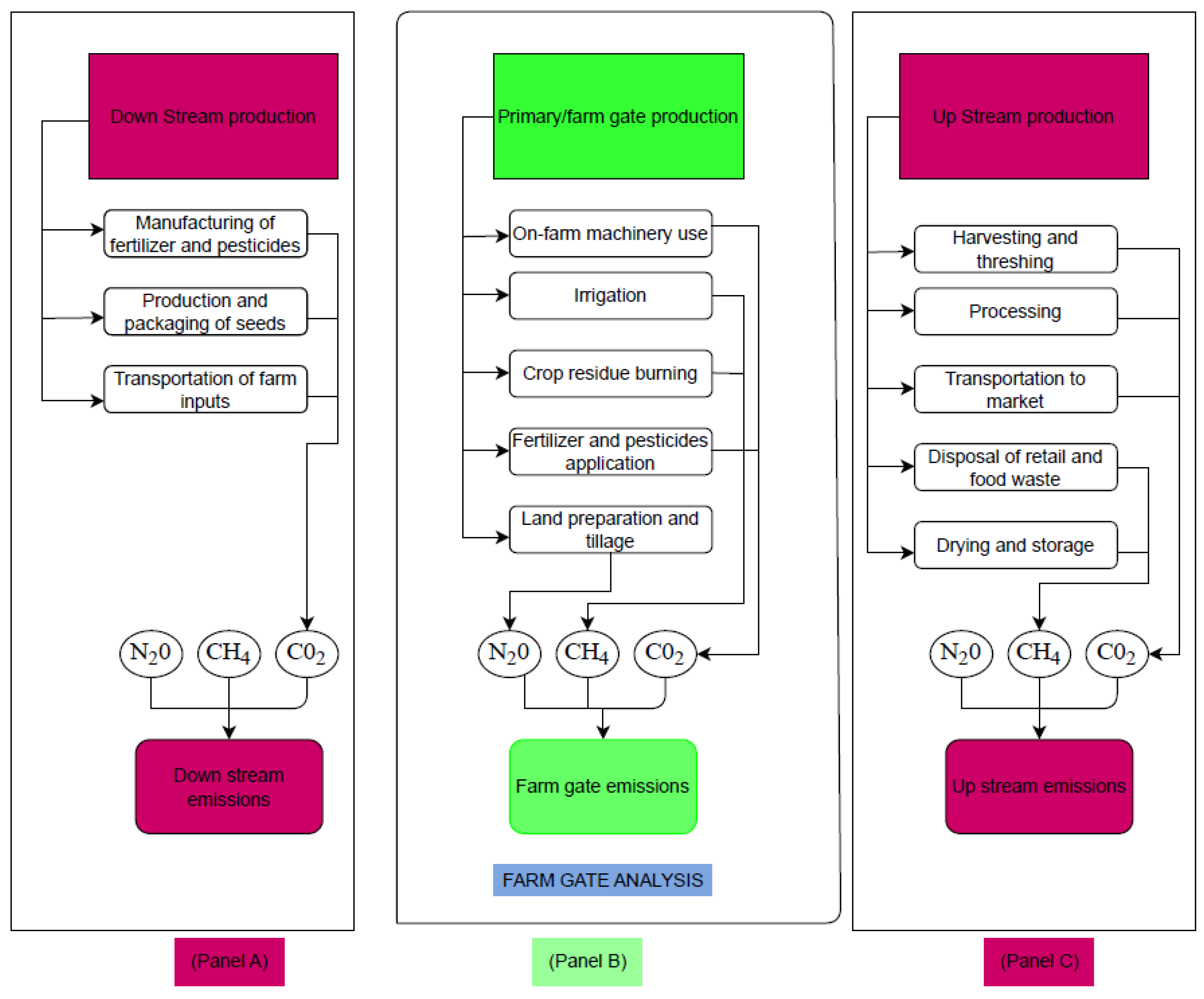
Figure 2.
The regression strategy. Source: Constructed by the Author.
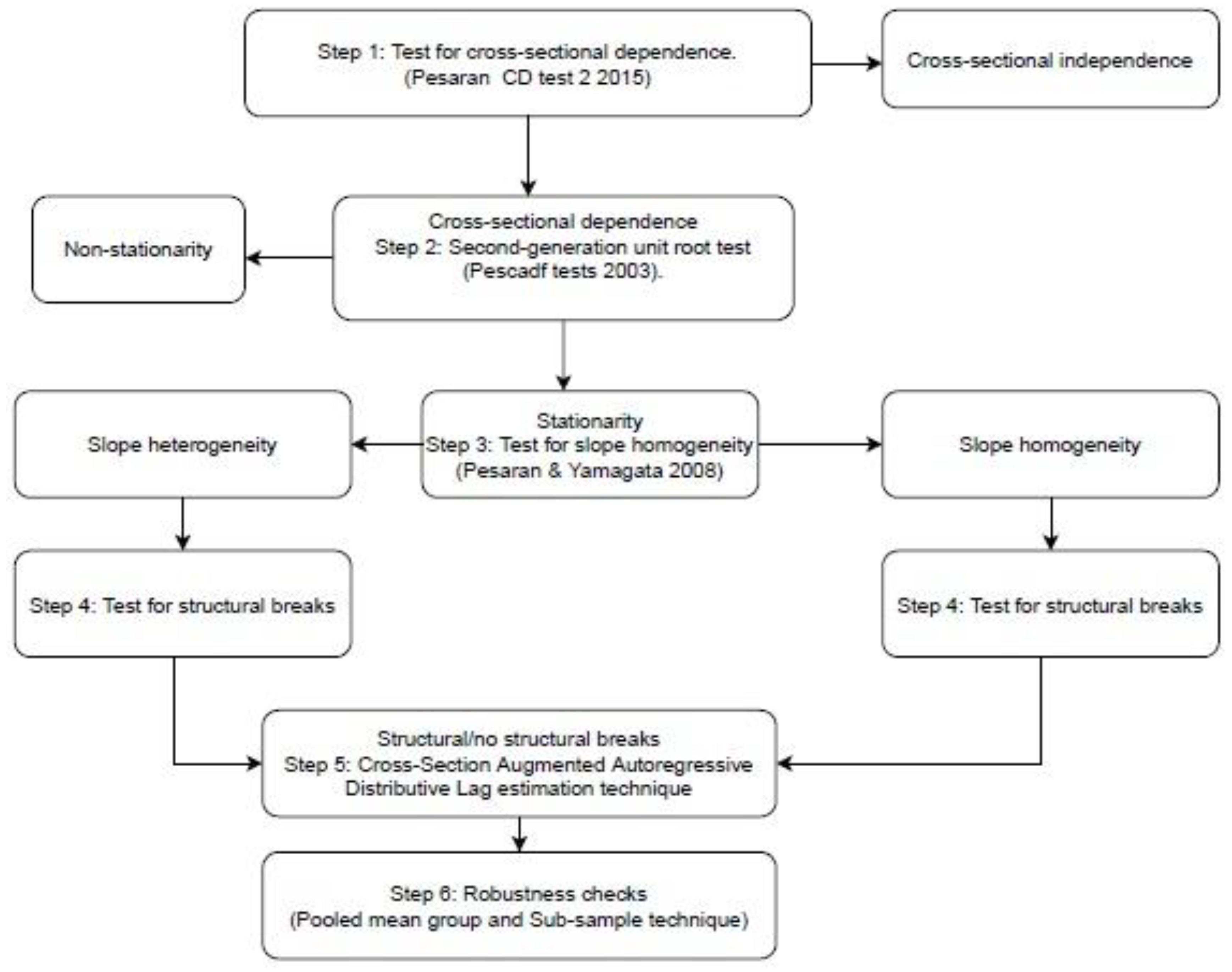
Figure 3.
Showing the share of crop production to the member state’s GDP in US$ million as of 2023. Source: Constructed by the Author.
Figure 3.
Showing the share of crop production to the member state’s GDP in US$ million as of 2023. Source: Constructed by the Author.
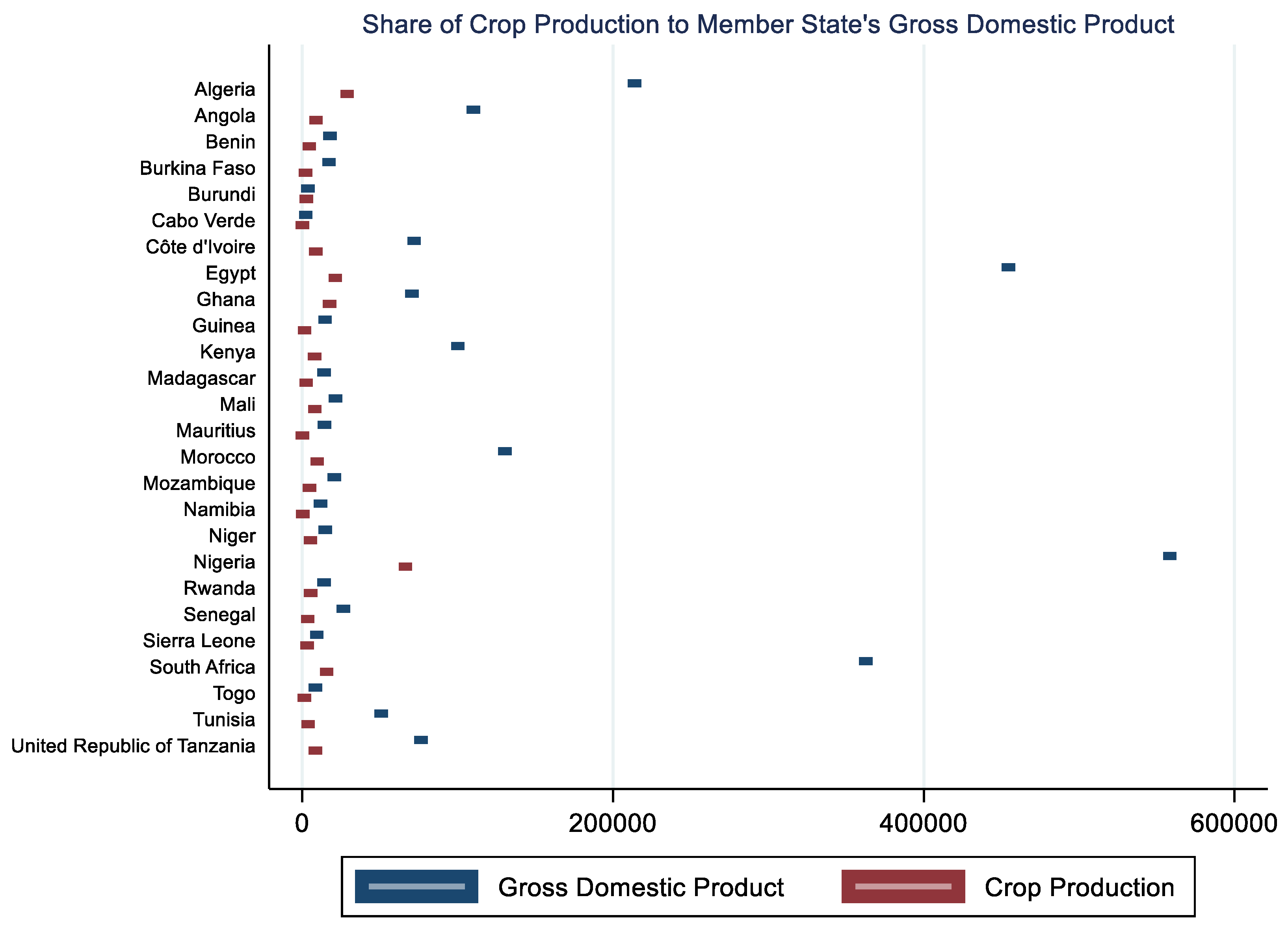
Figure 4.
Shows the percentage increase in crop production in each regional trading bloc member state. Every member is displayed by a small panel that illustrates the annual percentage growth for cereals, roots and tubers, vegetables, and fruits from 1990 to 2022. Source: Constructed by the Author.
Figure 4.
Shows the percentage increase in crop production in each regional trading bloc member state. Every member is displayed by a small panel that illustrates the annual percentage growth for cereals, roots and tubers, vegetables, and fruits from 1990 to 2022. Source: Constructed by the Author.
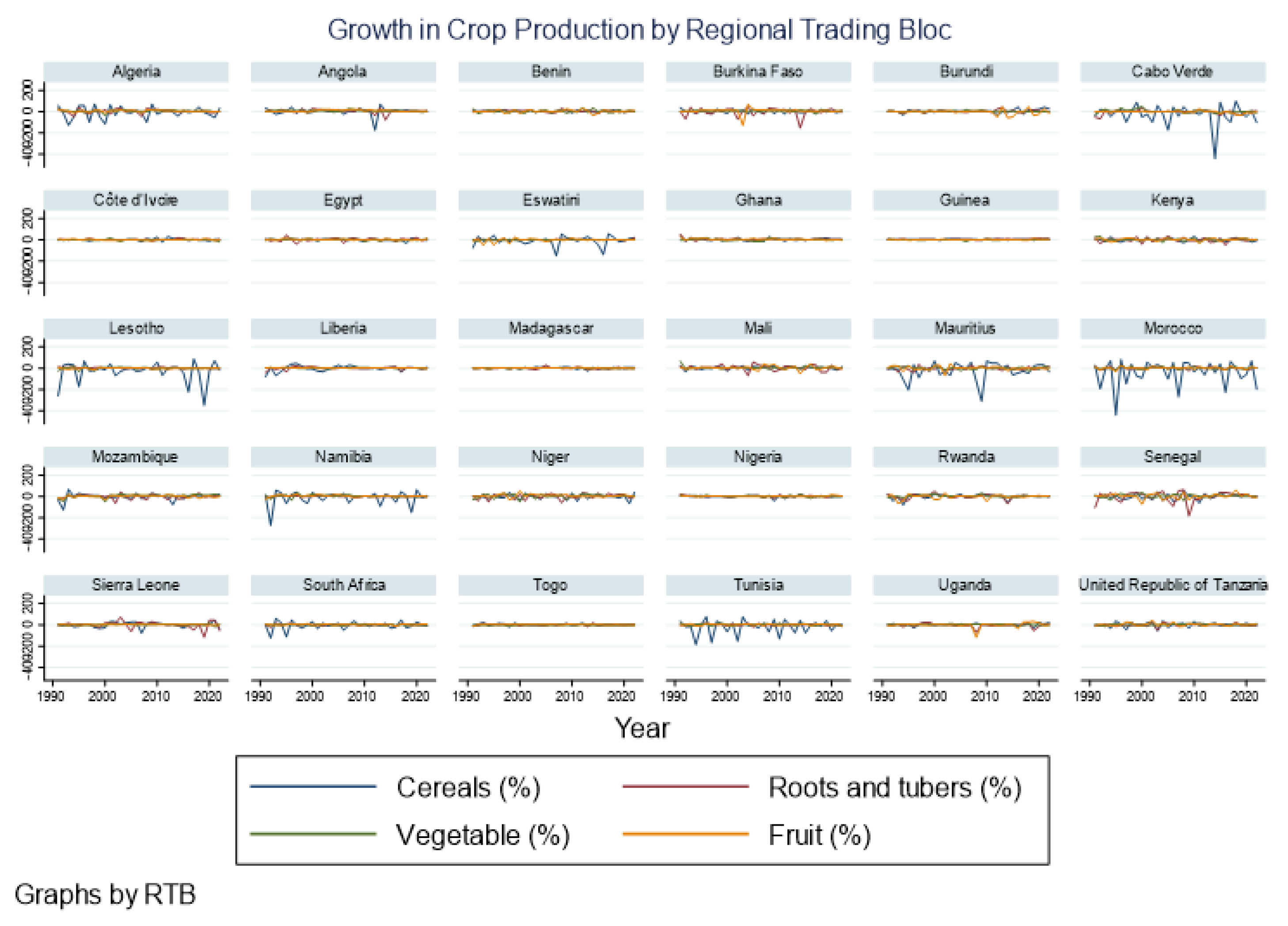
Figure 5.
The growth trends in N2O and methane CH₄ across Africa's RTB member states from 1990 to 2020 are depicted. The trajectory patterns display low to moderate variability, with notable variations in some member states of RTBs. Source: Constructed by the Author.
Figure 5.
The growth trends in N2O and methane CH₄ across Africa's RTB member states from 1990 to 2020 are depicted. The trajectory patterns display low to moderate variability, with notable variations in some member states of RTBs. Source: Constructed by the Author.
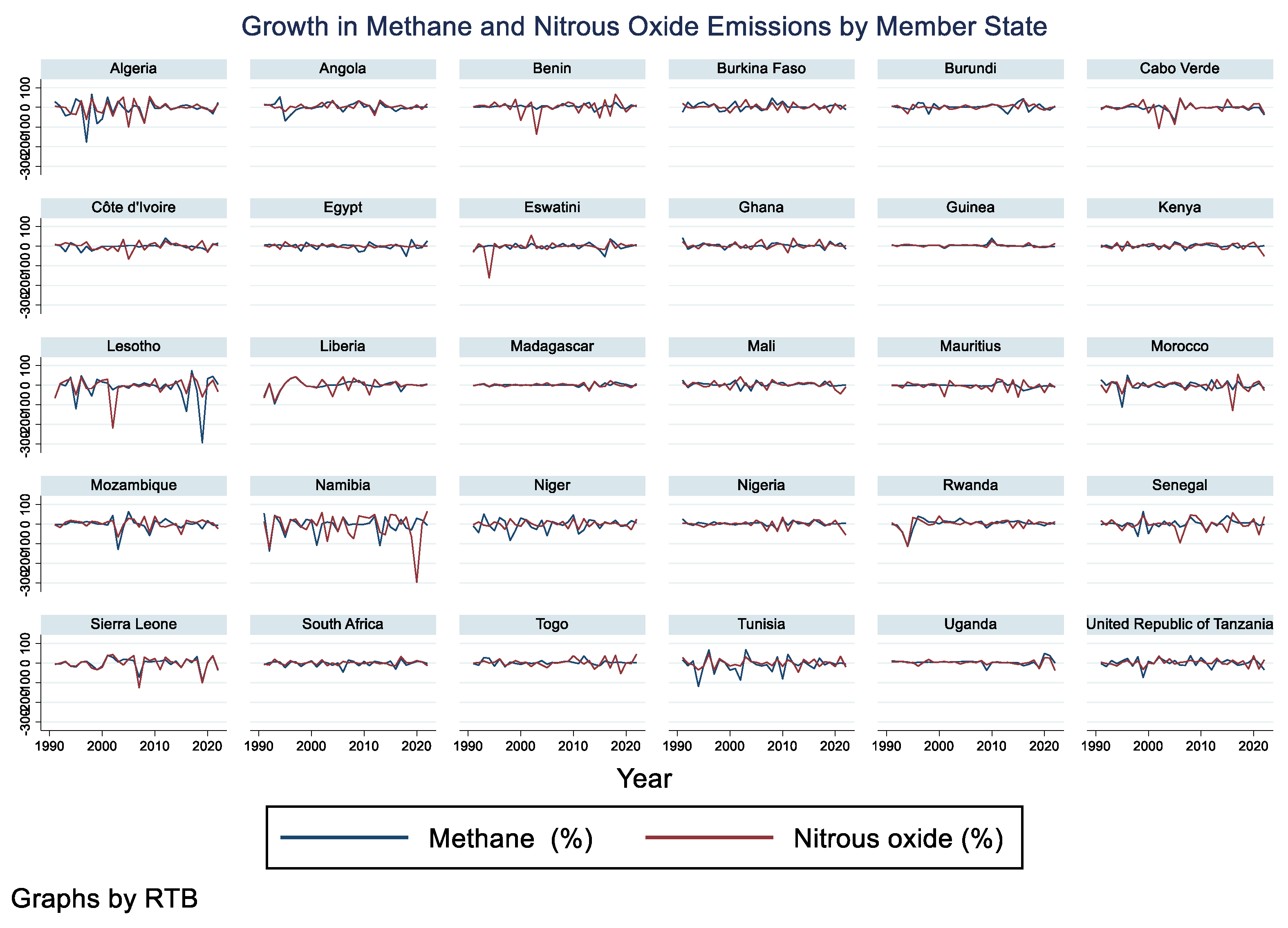
Figure 6.
The intensity of methane and nitrous oxide emissions from the various crops across the RTBs in Africa is compared. The intensity is the emission per output. Source: Constructed by the Author.
Figure 6.
The intensity of methane and nitrous oxide emissions from the various crops across the RTBs in Africa is compared. The intensity is the emission per output. Source: Constructed by the Author.
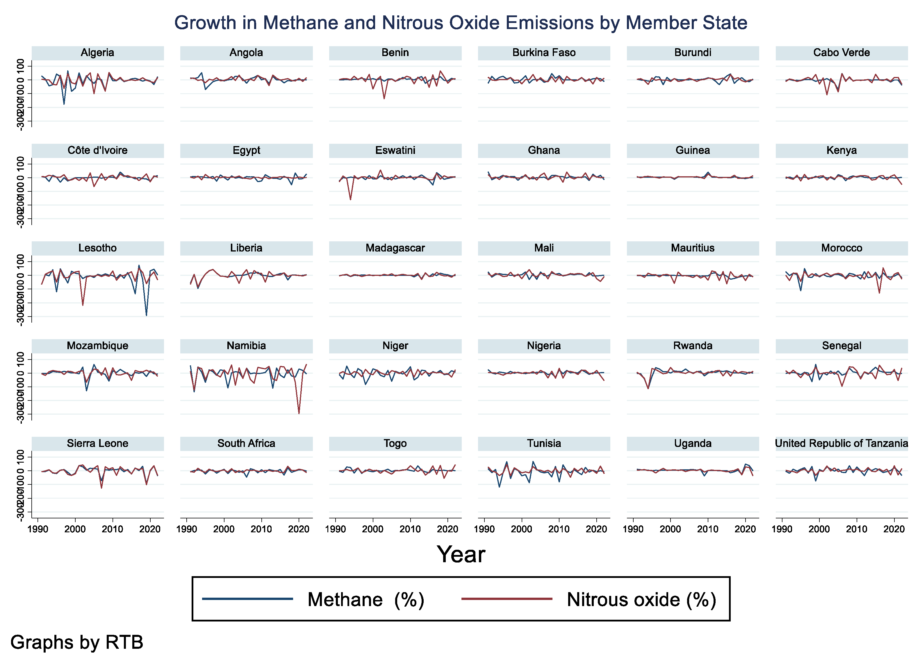
Table 1.
Member states of the regional trading blocs studied.
| S/n | Economic Community of West African States | South African Development Community | East African Community | The Maghreb |
|---|---|---|---|---|
| 1 | Benin | Angola | Burundi | Algeria |
| 2 | Burkina Faso | Eswatini | Kenya | Egypt |
| 3 | Cabo Verde | Lesotho | Rwanda | Morocco |
| 4 | Côte d'Ivoire | Madagascar | Tanzania | Tunisia |
| 5 | Ghana | Mauritius | Uganda | |
| 6 | Guinea | Mozambique | ||
| 7 | Liberia | Namibia | ||
| 8 | Mali | South Africa | ||
| 9 | Niger | |||
| 10 | Nigeria | |||
| 11 | Senegal | |||
| 12 | Sierra Leone | |||
| 13 | Togo |
Source: Constructed by the Author.
Table 2.
Variable Description.
| Variable | Description | Data source | Measurement | Reference |
|---|---|---|---|---|
| Methane | Emissions from agricultural activities such as burning residues and the cultivation of rice and other crops. | FAOSTAT | Kilotons |
[39,40] |
| Nitrous oxide | Emissions from agricultural activities, like irrigation and land use change. | [45,49] | ||
| Cereal | The primary output of all cereals at the farm-gate. | Metric tons | [39,42] | |
| Root and tuber | The total output of roots and tubers at the farm-gate. |
[43,45] | ||
| Vegetable | The primary output of vegetables at the farm-gate. | [46,47] | ||
| Fruit | The primary output of all fruits at the farm-gate. | [48,49] | ||
| Rural population | The total number of people that reside in the rural area per year |
Per thousand people. | [71] | |
| Technology | It encompasses the government expenditure, credit, development flows, and foreign direct investment in the agricultural sector. |
US$ million |
[72] |
Source: Computed by the Author.
Table 3.
Summary statistics.
| Variable | AMU | EAC | ECOWAS | SADC | Full sample | Means |
|---|---|---|---|---|---|---|
| Mean (Standard deviation) |
Mean (Standard deviation) |
Mean (Standard deviation) |
Mean (Standard deviation) |
Mean (Standard deviation) |
Highest Mean Difference (RTB) |
|
| Methane (In kilotons) | 307.29 (56.90) |
10.45 (3.50) |
574.89 (228.59) |
265.95 (31.36) |
38.62 (77.89) |
564.44 +, * (ECOWAS) |
| Nitrous oxide (In kilotons) | 42.13 (7.66) |
3.58 (1.31) |
23.12 (8.08) |
15.53 (29.00) |
2.81 (5.54) |
38.55 -, * (AMU) |
| Cereals (In million metric tons) | 41.4 (8.88) |
4.47 (1.05) |
48.1 (13.2) |
20.1 (4.95) |
3.80 (5 .81) |
43.7 +, * (ECOWAS) |
| Roots and tubers (In million metric tons) | 22.4 (5.16) |
7.80 (2.64) |
123.0 (45.6) |
20.4 (6.58) |
5.79 (16.0) |
115 +, * (ECOWAS) |
| Vegetables (In million metric tons) | 25.7 (7.66) |
2.73 (0.88) |
17.1 (6.44) |
4.39 (1.48) |
1.66 (3.18 |
23.0 -, * (AMU) |
| Fruits (In million metric tons) | 32.1 (8.64) |
7.174 (1.68 |
20.9 (6.55) |
9.967 (3.82) |
2.34 (3.15) |
24.9 -, * (AMU) |
| Rural population (Per million people) | 130.05 (22.28) |
45.04 (9.44) |
167.23 (26.71) |
61.16 (7.68) |
13. 45 (17 .08) |
122.19 +, * (ECOWAS) |
| Technology (In US$ billion) | 201.35 (126.10) |
15.58 (15.67) |
8.79 (86.12) |
113.26 (92.83) |
13 .94 (33. 77) |
185.77 -, * (AMU) |
Source: Computed by the Author Legend: (+) positive, and (-) negative mean differences, and * represents statistical significance. NOTE: Summary statistics for individual member states are in Appendix 1.
Table 4.
Test for cross-sectional dependence.
| Variable | CD test for methane | Variable | CD test for Nitrous oxide |
|---|---|---|---|
| Methane | 26.349a | Nitrous oxide | 55.142a |
| Cereals | 34.751a | Cereals | 34.751a |
| Roots and tubers | 52.788a | Roots and tubers | 52.788a |
| Vegetables | 55.012a | Vegetables | 55.012a |
| Fruits | 48.092a | Fruits | 48.092a |
| Rural population | 61.085a | Rural population | 61.085a |
| Technology | 80.315a | Technology | 80.315a |
Source: Computed by the Author Legend: a significant at 1%, b significant at 5%.
Table 5.
Pescadf unit root test for the methane model.
| Variables | Constant | Constant and trend | ||
|---|---|---|---|---|
| Level | First difference | Level | First difference | |
| Methane | -7.095a | -16.806a | -5.707a | -14.532a |
| Cereals | -5.751a | -17.52a | -4.699a | -15.825a |
| Roots and tubers | -1.413 | -15.427a | -1.893a | -13.645a |
| Vegetables | -2.461a | -12.72a | -0.161a | -7.596a |
| Fruits | -2.675a | -13.738a | -1.85a | -12.591a |
| Rural population | -13.496a | -7.413a | -6.75a | -7.037a |
| Technology | -1.321 | -14.068a | 1.468 | -12.282a |
Source: Computed by the Author Legend: a significant at 1%, b significant at 5%.
Table 6.
Pescadf unit root test for nitrous oxide model.
| Variables | Constant | Constant and trend | ||
|---|---|---|---|---|
| Level | First difference | Level | First difference | |
| Nitrous oxide | -2.991a | -16.515a | -2.326a | -14.148a |
| Cereals | -5.751a | -17.52a | -4.699a | -15.825a |
| Roots and tubers | -1.413 | -15.427a | -1.893a | -13.645a |
| Vegetables | -2.461a | -12.72a | -0.161a | -7.596a |
| Fruits | -2.675a | -13.738a | -1.85a | -12.591a |
| Rural population | -13.496a | -7.413a | -6.75a | -7.037a |
| Technology | -1.321 | -14.068a | 1.468 | -12.282a |
Source: Computed by the Author Legend: a significant at 1%, b significant at 5%.
Table 7.
Slope heterogeneity test for methane and nitrous oxide models.
| Methane | Nitrous oxide | |
|---|---|---|
| Delta | Delta | |
| 23.768a | 16.384a | |
| Adjusted delta | 27.371a | 18.867a |
Source: Computed by the Author Legend: a significant at 1%, b significant at 5%.
Table 8.
Bai & Perron test for structural breaks.
| Methane | Nitrous oxide | |||||
|---|---|---|---|---|---|---|
| F(1/0) | F(2/1) | F(3/2) | F(1/0) | F(2/1) | F(3/2) | |
| T – Statistic | 1.71 | 2.26 | 2.39 | 2.62 | 6.97 | 6.62 |
| 1% Critical value | 5.69 | 6.24 | 6.53 | 5.69 | 6.24 | 6.53 |
| 5% Critical value | 4.35 | 4.88 | 5.2 | 4.35 | 4.88 | 5.2 |
| 10% Critical value | 3.72 | 4.32 | 4.65 | 3.72 | 4.32 | 4.65 |
| Detected number of breaks: | 0 | 0 | 0 | 3 | 3 | 3 |
Source: Computed by the Author Three cases: cereals, roots, and tubers, and fruit are considered due to the length of the period being less than the number of variables. The lag of the cases is taken into account for the dynamism of the model. The cross-sectional means of the first difference of the lag of the cases are incorporated to account for cross-sectional dependence and the standard error [91] for the robustness of the result: Set trimming to 0.25 for at most 3 breaks.
Table 9.
CS-ARDL Crop production and methane emissions results.
| Variable | Short-run elasticity coefficient |
Short-run proportional change coefficient |
Long-run elasticity coefficient | Long-run proportional change coefficient |
|---|---|---|---|---|
| Cereals | 0.4746a | 1.0021 | 0.7739a | 1.0033 |
| (-0.0838) | (-0.2882) | |||
| Roots and tubers | -0.1425 | 0.9994 | -0.162 | 0.9993 |
| (-0.1657) | (-0.1808) | |||
| Vegetables | 0.1651 | 1.0007 | 0.2923 | 1.0013 |
| (-0.1059) | (-0.2462) | |||
| Fruits | 0.4472a | 1.0019 | 0.5403a | 1.0023 |
| (-0.1394) | (-0.192) | |||
| Rural population | -0.1045 | 0.9995 | -0.3394 | 0.9985 |
| (-0.4731) | (-0.581) | |||
| Technology | -0.0152 | 0.9999 | -0.0234 | 0.999 |
| (-0.0244) | (-0.0319) | |||
| Lag of emissions | 0.1336a | |||
| (-0.05) | ||||
| Error correction term | -0.8664a | |||
| (0.4998) | ||||
| F-statistic | 2.78a | |||
| Number of observation | 949 | |||
| Number of member states | 30 | |||
Source: Computed by the Author Legend: a significant at 1%, b significant at 5%, standard error in parentheses.
Table 10.
CS-ARDL Crop production and nitrous oxide emissions results.
| Variable | Short-run elasticity coefficient | Short-run proportional change coefficient |
Long-run elasticity coefficient |
Long-run proportional change coefficient |
|---|---|---|---|---|
| Cereals | 0.5229a | 1.0024 | 0.8115a | 1.0035 |
| (-0.1096) | (-0.2442) | |||
| Roots and tubers | 0.2877 | 1.0012 | 0.3939 | 1.0017 |
| (-0.3431) | (-0.5061) | |||
| Vegetables | 0.0251 | 1.0001 | 0.1252 | 1.0005 |
| (-0.1343) | (-0.1647) | |||
| Fruits | 0.5784b | 1.0025 | 0.6375 | 1.0028 |
| (-0.2903) | (-0.5519) | |||
| Rural population | 0.9891 | 1.0043 | 0.6514 | 1.0028 |
| (-1.29) | (-1.5189) | |||
| Technology | 0.0131 | 1.0001 | 0.0089 | 1.0000 |
| (-0.016) | (-0.234) | |||
| Lag of emissions | 0.1578a | |||
| (-0.0439) | ||||
| Error correction term | -0.8422a | |||
| ( -0.0439) | ||||
| F-statistic | 1.44a | |||
| Observation | 949 | |||
| Member states | 30 | |||
Source: Computed by the Author Legend: a, significant at 1%, b significant at 5%, standard error in parentheses.
Table 11.
PMG Crop production and methane emissions results.
| Variable | Short-run elasticity coefficient | Short-run proportional change coefficient |
Long-run elasticity coefficient | Long-run proportional change coefficient |
|---|---|---|---|---|
| Cereals | 0.2971a | 1.0013 | 0.3156a | 1.0014 |
| (-0.0634) | (-0.046) | |||
| Roots and tubers | 0.0548 | 1.0002 | -0.0524 | 0.9998 |
| (-0.0675) | (-0.0383) | |||
| Vegetables | 0.1134 | 1.0005 | -0.0854b | 0.9996 |
| (-0.089) | (-0.0405) | |||
| Fruits | 0.2068 | 1.0009 | 0.2171a | 1.0009 |
| (-0.1284) | (-0.0427) | |||
| Rural population | -3.5268 | 0.9849 | 1.1926a | 1.0052 |
| (-5.5204) | (-0.1126) | |||
| Technology | -0.0025 | 1.0000 | -0.0240b | 0.9999 |
| (-0.0096) | (-0.0109) | |||
| Error correction term | -0.3925a | |||
| (-0.0523) | ||||
| Number of observation | 949 | |||
| Member states | 30 | |||
Source: Computed by the Author Legend: a significant at 1%, b significant at 5%, standard error in parentheses.
Table 12.
PMG Crop production and nitrous oxide emissions results.
| Variable | Short-run elasticity coefficient | Short-run proportional change coefficient | Long-run elasticity coefficient | Long-run proportional change coefficient |
|---|---|---|---|---|
| Cereals | 0.2921a | 1.0013 | 0.4077a | 1.0018 |
| (-0.0861) | (-0.0438) | |||
| Roots and tubers | 0.246 | 1.0011 | 0.049 | 1.0002 |
| (-0.2246) | (-0.0364) | |||
| Vegetables | 0.1199 | 1.0005 | 0.0359 | 1.0002 |
| (-0.1106) | (-0.0392) | |||
| Fruits | 0.0376 | 1.0002 | 0.1683a | 1.0007 |
| (-0.1161) | (-0.028) | |||
| Rural population | 4.9843 | 1.0218 | 0.7300a | 1.0032 |
| (-2.71466) | (-0.0949) | |||
| Technology | 0.0286a | 1.0001 | 0.014 | 1.0001 |
| (-0.0103) | (-0.0144) | |||
| Error correction term | -0.44144a | |||
| (-0.0586) | ||||
| Number of observation | 949 | |||
| Member states | 30 | |||
Source: Computed by the Author Legend: a significant at 1%, b significant at 5%, standard error in parentheses.
Table 13.
Sub-sample crop production and methane emissions results.
| Variable | Short-run elasticity coefficient | Short-run proportional change coefficient |
Long-run elasticity coefficient |
Long-run Proportional change coefficient |
|---|---|---|---|---|
| Cereals | 0.2773a | 1.0012 | 0.3460a | 1.0015 |
| -0.0606 | -0.0746 | |||
| Roots and tubers | -0.1753 | 0.9992 | -0.2123 | 0.9991 |
| -0.2596 | -0.37 | |||
| Vegetables | -0.1113 | 0.9995 | -0.0872 | 0.9996 |
| -0.2973 | -0.376 | |||
| Fruits | 0.5366b | 1.0023 | 0.6454a | 1.0028 |
| -0.2485 | -0.2146 | |||
| Rural population | 1.1224 | 1.0049 | 1.1282 | 1.0049 |
| -1.0674 | -1.088 | |||
| Technology | -0.0436 | 0.9998 | -0.0926 | 1.0004 |
| -0.0369 | -0.0572 | |||
| Error correction term | -0.8383a | |||
| -0.1247 | ||||
| F-statistic | 2.47a | |||
| Number of observations | 251 | |||
| Member states | 8 | |||
Source: Computed by the Author Legend: a significant at 1%, b significant at 5%, standard error in parentheses.
Table 14.
Sub-sample crop production and nitrous oxide emissions results.
| Variable | Short-run elasticity coefficient | Short-run proportional change coefficient |
Long-run elasticity coefficient |
Long-run proportional change coefficient |
|---|---|---|---|---|
| Cereals | 0.2847a | 1.0012 | 0.3504a | 1.0015 |
| (-0.0636) | (-0.0755) | |||
| Roots and tubers | 1.1939 | 1.0052 | 1.359 | 1.0059 |
| (-1.1946) | (-1.3875) | |||
| Vegetables | -0.5678 | 0.9975 | -0.6273 | 0.9973 |
| (-0.3646) | (-0.3695) | |||
| Fruits | 0.1716 | 1.0007 | 0.2329 | 1.001 |
| (-0.6635) | (-0.7807) | |||
| Rural population | 3.4435 | 1.015 | 4.0475 | 1.0176 |
| (-2.3565) | (-2.807) | |||
| Technology | 0.0784 | 1.0003 | 0.0863 | 1.0004 |
| (-0.0677) | (-0.0763) | |||
| Error correction term | -0.8568a | |||
| (-0.0539) | ||||
| F-statistic | 1.08 | |||
| Number of observations | 251 | |||
| Member states | 8 | |||
Source: Computed by the Author Legend: a significant at 1%, b significant at 5%, standard error in parentheses.
Disclaimer/Publisher’s Note: The statements, opinions and data contained in all publications are solely those of the individual author(s) and contributor(s) and not of MDPI and/or the editor(s). MDPI and/or the editor(s) disclaim responsibility for any injury to people or property resulting from any ideas, methods, instructions or products referred to in the content. |
© 2025 by the authors. Licensee MDPI, Basel, Switzerland. This article is an open access article distributed under the terms and conditions of the Creative Commons Attribution (CC BY) license (http://creativecommons.org/licenses/by/4.0/).
Copyright: This open access article is published under a Creative Commons CC BY 4.0 license, which permit the free download, distribution, and reuse, provided that the author and preprint are cited in any reuse.


