Submitted:
31 August 2025
Posted:
01 September 2025
You are already at the latest version
Abstract
Pegging warming to 1.5 degrees Celsius requires a considerable reduction in greenhouse gas emissions through technological advancement. However, the role played by technology in mitigating emissions has attracted less attention in the agricultural sector. This novel study examines the effect of agricultural spending on technology on agricultural greenhouse gas emissions in 29 selected regional trading bloc member states in Africa. We adapted the Kaya Identity model to the agricultural sector by equating technology to expenditure on capital goods and research and development. We collected secondary data from 1993 to 2022. We analyzed the adapted Kaya Identity model using the fully modified ordinary least squares method and the canonical co-integration regression technique for a robustness check. The results revealed that agricultural spending on capital goods plays a moderately significant role in mitigating agricultural greenhouse gas emissions. We recommend that the member states increase the budget for green agriculture and incentivize clean technology investments. At the regional trading bloc level, we recommend the crafting, implementation, or strengthening of the regional trading blocs' emissions control plans.
Keywords:
adapted Kaya identity
; agricultural greenhouse gas emissions
; agricultural spending on capital goods
; agricultural spending on research and development
; regional trading blocs
1. Introduction
Agricultural spending on technology (AST) is increasingly important to enhance production and ensure food security, especially with the rising population’s growing demand for food [1]. In Africa, with the agricultural sector at the center of the transformation of the continent’s economy, which is potentially a powerhouse globally and a net food exporter [2], AST is critical to increase the volume of output. Thus, AST serves as an engine for growth.
To enhance growth in the agricultural sector, African countries made commitments under the Comprehensive African Agriculture Development Program (CAADP) to spend at least ten percent of their budget on the agricultural sector [3].
These African countries are members of regional trading blocs (RTBs) to increase their exports by lessening trade protection on one another’s exports [4]. This further puts upward pressure on their expenditure to boost production and trade [5].
Consequently, the ratio of member states' expenditure to gross domestic product (GDP) in the agricultural sector, especially in 2023, experienced an overall increase of eight percent. The Arab Maghreb Union (AMU) incurred the highest spending in the agricultural sector (6.2%), followed by SADC (6.1%).
The Economic Community of West African States (ECOWAS) spent the least, 2.8%, while the East African Community (EAC) agricultural expenditure was 4%. In this regard, the 2022 assessment of the progress made after the CAADP’s commitment by these member states in 2014 depicts an annual average percentage change in agricultural output of approximately 2.6%; with the ECOWAS having an annual average percentage change of 3.2%, the EAC 3.0%, the SADC 2.6%, and the AMU 1.5% [6].
This growth agricultural output comes at the expense of emissions. In 2022, Africa’s agricultural sector contributed approximately 8% of the world’s carbon dioxide equivalent emissions, with the AMU, the EAC, the ECOWAS, and the SADC contributing 16%, 33%, 15%, and 36%, respectively, to the continent’s agricultural greenhouse gas emissions (AGEs) [7]. With Africa’s growing interest in trade, the contribution of RTB agriculture-based emissions is most likely to rise; resulting in environmental degradation.
Climate change effects are far-reaching; they threaten the livelihood of small-scale farmers, particularly the poorest and vulnerable rural population [1] by causing an economic loss of 7% to 10% of a country's GDP [8].
The increasing adverse effects of climate change, particularly in the agricultural sector, have called for urgent action by countries to mitigate its threat [9]. In this regard, the SADC, for instance, developed a framework for reducing the vulnerability of the key agricultural subsector to the effects of climate change. It also strengthened the research and development capacity in the region [10] to identify AGE drivers and mitigate them. In addition, at the member state level, nations have agreed to set emissions at 1.5 degrees Celsius [11]. We ask: Are these RTB member states’ strides reducing AGEs? Hence, this paper examines the effect of AST on AGEs in the major regional trading bloc member states in Africa.
The specific objectives are to: (i) determine the effect of agricultural spending on capital goods (ASCGs) on AGEs in the regional trading bloc member states in Africa, and (ii) analyze the effect of agricultural spending on research and development (ASRD) on AGEs in the trading bloc member states in Africa.
Empirically, researchers have attempted to investigate the contribution of AST in mitigating emissions. Perhaps the closest study to our work is by [12]. He examined the effect of public agricultural spending on AGEs in Africa while controlling for foreign direct investment and official development assistance in the agricultural sector. He specified a static-level model using variables drawn from various literature and used the instrumental variable technique for estimation. His results showed that a rise in agricultural public expenditure increased AGEs.
This study deviates from Diop’s work and, as a result, makes four contributions. First, we examine AST by all players as a group to get the total effect that AST will have on AGEs. Second, we develop our model based on the Kaya identity theory rather than a review of past literature; which will aid the robustness of the tested hypotheses and the generalization of our regression results.
Also, we adapted the Kaya identity, especially technology, to mean AST and split AST into ASCGs and ASRD. Thus, from the generated results, we can design a coordinated policy to regulate AST and efficiently allocate the scarce agricultural resources of RTB member states into either ASCGs or ASRD, or both.
Third, instrumental variable estimation technique does not account for the long-run relationship; which is critical as AST, especially ASRD, lags because it takes time for these expenditures to translate into tangible outcomes. Thus, we employ the fully modified ordinary least squares (FMOLS) approach to co-integration and the canonical co-integration regression (CCR) as a robustness check, which controls for serial correlation, endogeneity, and determines long-run relationships. Hence, accounting for the gestation period of AST and, as such, showing its true potential.
Fourth, this study focuses on the RTBs where existing structures and policies to mitigate AGEs exist, rather than geography or income level. Thus, this study output will be pertinent to the RTBs in terms of independent assessment of the strides they have made in mitigating AGEs and as a basis for future trade and emissions policy design and implementation of an extended RTB, such as the African Continental Free Trade Area (AfCFTA).
2. Conceptualization and Hypothesis
2.1. Agricultural Spending on Capital Goods and Agricultural Greenhouse Gas Emissions
In a broad sense, capital goods are durable assets that are used to produce other goods or services. They include goods such as infrastructure, tools, buildings, and equipment, which are not directly sold to consumers [13]. Capital goods are inputs in the production process and, as such require producers to expend on them.
Such expenditure is referred to as capital expenditure. Thus, in the agricultural sector, capital expenditure may mean ASCGs, which represent agricultural investments from development partners, the government, and the private sector in physical agricultural assets such as machinery, irrigation systems, equipment, and storage facilities that help farmers to enhance productivity and reduce emissions per unit of agricultural output [14] through the adoption of more efficient agricultural practices such as efficient use of energy [15] and the improvement in the accuracy of the combination of input (such as fertilizer and water) used [16].
Evidence from Chinese provinces has shown that agricultural fiscal spending for the improvement of technological advancement can significantly reduce agricultural carbon emissions [17]. Similarly, [18] suggested that the intensive use of energy in an industrialized system reduces per-unit emissions of agricultural output. Conversely, agricultural machinery intensity reduces the efficiency of agricultural carbon emissions in China [19]. Based on the mixed results obtained, we propose the following hypothesis:
Hypothesis 1:
Agricultural spending on capital goods significantly increases agricultural greenhouse gas emissions in Africa’s regional trading blocs.
2.2. Agricultural Spending on Research and Development and Agricultural Greenhouse Gas Emissions
Broadly speaking, research and development refers to a systematic process to expand knowledge and the application of such expertise to drive innovation, such as the development of a new product or technology [20]. R&D is an intangible asset classified as expenditure because it represents a cost to producers [21]. R&D costs incurred by producers in the agricultural sector may be referred to as ASRD.
The ASRD encompasses public, private, and donor partners’ investments in innovation, the development of new technologies, and the acquisition of knowledge aimed at transforming agricultural practices to increase productivity and lower emissions [22,23]. This spending can be in the form of developing climate-smart agricultural practices and technologies, such as low-emissions crops and livestock, methane-reducing feeds, novel organic fertilizer substitutes for chemical fertilizers, and digital tools [24].
We cannot underestimate the importance of ASRD in mitigating AGEs, as an increase in investment in public research and development (R&D) in the livestock sub-sector can reduce AGEs [25].
In addition, additional Investment in R&D to boost agricultural productivity can also lower AGEs from changing land use [17]. Moreover, the tripling of public R&D expenditures in the agricultural sector, combined with policies directed to mitigate emissions, will not only increase agricultural productivity, but also result in significant mitigation of AGEs in the United States of America [26]. With these insights, we hypothesize the following:
Hypothesis 2:
Agricultural spending on research and development significantly increases agricultural greenhouse gas emissions in Africa’s regional trading blocs
3. Methodology
3.1. Estimation Strategy
In this study, we test whether a static or dynamic model should be specified by estimating our equation using the lag of the explained variable as an explanatory variable. A statistically significant probability value of the lag variable shows that the lag of the explained variable (AGEs) is correlated with the explained variable. Hence, a dynamic model should be specified, and a static model otherwise.
We also use the [27] test for cross-sectional dependence (CD) to inform the use of the appropriate panel unit root test for stationarity of the regression variables because it is more applicable for balanced and unbalanced panels. We adopted the [28] test to confirm the results. Thereafter, we test for the stationarity of the variables using [29] first-generation unit root test, in the absence of CD, and the second-generation unit root test otherwise. We used the [30] co-integration test to confirm the long-run relationship between the variables, assuming across-panel CD is non-existent, which is confirmed by the [31] co-integration test.
We also test for homogeneity in slope for the model [32] to determine whether the results of the individual cross-sections should be displayed or the aggregate results. In the presence of a long-run relationship, we employ the FMOLS proposed by [33] to estimate the long-run model because it is efficient in dealing with the problem of serial correlation and endogeneity [34]. The CCR propounded by [35] is also employed as a robustness check. We use Stata 17 [36] for our empirical analysis.
3.2. Adapted Kaya Identity Model
Many researchers have developed several theories of climate change, such as the environmental impact of population, affluence, and technology (IPAT), the Stochastic Impacts by Regression on Population, Affluence, and Technology (STIRPAT), and the environmental Kuznets curve (EKC) hypothesis. However, these models are limited for adaptation in this study. The IPAT model is limited due to its inability to visibly show, using regression, the stochastic effect of population, affluence, and technology on the environment [37]. The STIRPAT model is complex because of the introduction of the stochastic term and non-unit elasticity on the impact of each driving force on environmental degradation [38]. The major EKC weakness, among others, is that it only considers gross domestic product and environmental degradation and concentrates on a single country [39]. Thus, we use the Kaya Identity Model (KIM) in this study to analyze the effect of AST on AGEs in the RTBs in Africa.
Climate change threatens the environment, and agricultural production is one of the major culprits. Since countries need to feed their populations, it becomes apparent that they should not halt production to peg AGEs, but rather find ways to meet their population demand for food, and at the same time reduce emissions. Thus, the KIM provides that framework by specifying factors such as population, gross domestic product, and technology that are key drivers of AGEs.
The reason for using this model is that it is a simple model, and it pays special attention to the technological factor as a driver of emissions. It separates technology into energy efficiency and the emission factor, which is adapted in this study to mean ASCGs and ASRD, respectively. The KIM is a dynamic model that can be applied to national and regional studies. Thus, on a regional basis, the KIM captures the variation of rural population (RP), agricultural output per capita (AOPC), ASCGs, and ASRD in the various member states of the blocs under consideration.
3.3. Empirical Model Specification
The KIM serves as the theoretical basis for simulating AGEs. A straightforward mathematical model called the KIM breaks down the variables affecting carbon dioxide (CO2) emissions [40]. It is often applied in the context of energy and climate policy analysis to understand the drivers of emissions and explore potential pathways to reduce them.
While researchers such as [41] primarily used the KIM to analyze emissions and understand their driving factors, they did not accurately adapt the theory to the agricultural sector because they did not split the technology components of the KIM in their adaptation. For the correct modification of the KIM to the agriculture sector, the model in its simplest form is given as carbon dioxide emission is a product of the population multiplied by affluence multiplied by technology (divided into energy efficiency and emission factor) [40]. Thus, the KIM is given as:
where c is world CO2 emissions; p is world population growth; g is world GDP; e is world energy consumption, (g/p) is the per capita economic activity, energy efficiency, and emission factor.
AST comprises ASCGs and ASRD. The ASCGs are assumed to be expenditure on technologies that require less energy consumption and provide the efficient energy needed to produce agricultural output. Hence, it is used as an energy efficiency proxy. The ASRD assumes expenditure on new technology, knowledge, and innovation that emit less CO2 in producing agricultural output. Thus, we proxy the emission factor to imply ASRD.
Agricultural production mainly takes place in the rural areas. The rural areas accounted for roughly 57 percent of the total population of Sub-Saharan African countries in 2023 [42]. Thus, we proxy the population to imply the rural population (RP). Furthermore, we proxy the per capita economic activity by agricultural output per capita (AOPC) and CO2 emissions as AGEs because the study focuses on the agricultural sector. Hence, equation (3.1) is rewritten as:
Equation 3.2 shows the direct effect the AST will have on AGEs. However, since ASRD especially lags, we consider the lagged structure of ASCGs, ASRD, and other variables in the model when examining the effect of AST on AGEs using elasticity [43]. Specifying equation (3.2) in double log panel econometric form yields:
where is the natural logarithm (elasticity), are the parameters to be estimated, is the error term, represents countries, and ‘t’ means time.In
addition, with AGEs changing over time, past emission measurements will likely
be correlated with the present. Hence, we specify a dynamic panel model by
including the lag of AGEs as an independent variable [44].
Therefore, we rewrite (3.3) as:
3.4. Data
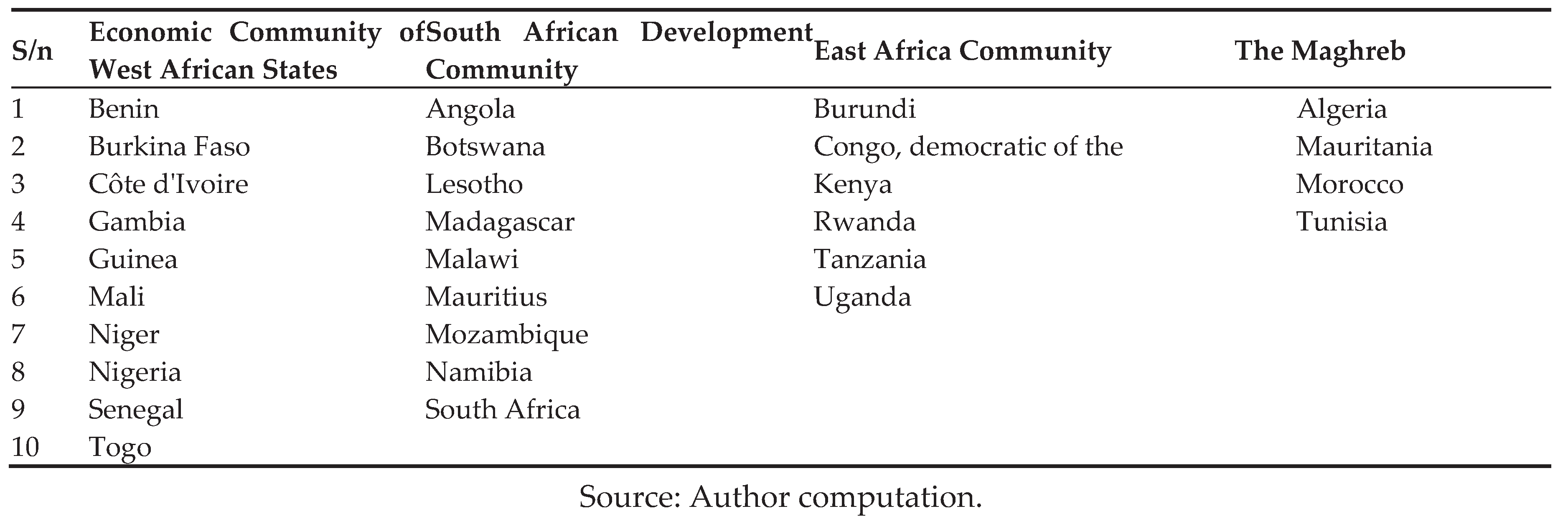
There are several RTBs in Africa due to the aims and aspirations of countries to increase the volume of trade; which affects the agricultural sector’s emissions. However, we consider only the major RTBs (based on membership) from each of the four regions (to avoid duplication of member states). That is, AMU in the north, EAC in the east, ECOWAS in the west, and SADC in the south, because they have the largest number of member states in their respective geographical regions.
As a result, we drew forty-two (42) countries and selected 29 member states (See Appendix A1) that belong to the AMU, EAC, ECOWAS, and SADC based on data availability. We collected data for the variables from the Food and Agriculture Organization Statistics (FAOSTAT) [7] https://www.fao.org/faostat/en/#data, and agricultural science and technology indicators (ASTI) [45] https://www.asti.cgiar.org/data databases from 1993 to 2022 (see Table 1)
3.5. Estimation Technique
From equation (3.4), we specify a dynamic model, so the use of static models like fixed-or random-effects estimators is inconsistent as, by construction, they are linked with the unobserved panel effects that provide misleading inferences. Thus, to estimate consistent estimates, more sophisticated dynamic panel data estimators are needed [48]. Consequently, the generalized method of moments (GMM) estimator was posited to solve the endogeneity problem by employing all possible lagged values of the endogenous variable as instruments [49]. However, its weakness is that it solely utilizes time and not cross-sectional variation. To prevent this information loss, the System GMM is adopted.
The GMM and system GMM are employed for large cross-sectional units with a short time. The inapplicability of these estimation methods for large time and cross-section series results in the use of the mean group (MG) and pooled mean group (PMG) estimation techniques. The Mean Group estimator [50] posits that each cross-sectional unit can be estimated separately and examines how the estimated coefficients across the cross-sectional units are distributed.
The model's weakness is that it ignores certain parameters that might apply to all the cross-sectional units [51]. According to [51], the Pooled MG (PMG) estimator permits group short-run coefficients and error variances while restricting long-run coefficients to be the same. This estimation technique is superior to the MG because cross-sectional units can be pooled and averaged. The PMG is limited in analyzing long-run relationships between variables. Thus, this problem is addressed using dynamic ordinary least squares (DOLS) and FMOLS [34]. However, while the application of the DOLS follows rules such as variable stationarity and co-integration, the FMOLS does not, because it is non-parametric [52]. Hence, we employ the FMOLS technique to estimate our regression model because it is unaffected by standard ordinary least squares properties.
3.6. The Fully Modified Ordinary Least Squares Model
The panel model, which is a generalization of the work of [33] serves as the foundation for the group-mean panel FMOLS approach [34] presented as:
where x denotes an array of independent variables, and y represents the dependent variable.
In this case, error terms e and ε are acknowledged as stationary. The following is an estimation method for the panel FMOLS estimator for the β estimator:
Where
where is the FMOLS estimated parameter. demonstrates a long-run covariance matrix, where is a weighted sum of covariance and is the contemporaneous covariance. The lower triangular matrix in the breakdown of is .
3.7. Conversion of Emissions’ Elasticity to Proportional Change
The estimated coefficients are in elasticity because the model is specified in double log form to capture the lag of especially, ASRD and the other independent variables. However, since changes in emissions are typically measured yearly, we represent AGEs in their original form [53]. Following the work of [54], the proportional change in emissions as a result of a percent increase in the driving forces of emissions is given as;
Where is the exponent,, the expected increase in emissions, is the estimated regression coefficient, is the magnitude of the change (q = 1%).
4. Results and Discussion
4.1. Descriptive Results
In this study, we use the full sample average of the RTBs as a benchmark to explain the changes observed in these RTBs. According to Table 2, the high-emitting RTBs in Africa are SADC and EAC, which accounts for 682 709.70 kilotons and 562 248.50 kilotons of AGEs, respectively, on average in a year.
The ECOWAS’ AGEs is moderate (256 886.60 kilotons), while the AMU emits the least (187 551.00 kilotons) on average per year. The SADC’s high emissions may be due to its high capital expenditure (US$ 1527.72 million) and output per head (US$ 422 900). Thus, suggesting the expenditure on high-level emission technologies to increase agricultural output per leads to higher emissions. Similarly, the high emissions from the EAC depict the unfriendly emissions practices adopted by its high rural population (140 938.00 per thousand) in producing for subsistence.
Furthermore, the ECOWAS moderate emissions are due to the blend of its high rural population (154 659.10 per thousand) and moderate expenditure on capital goods (US$ 706.41 million). The AMU is the most environmentally friendly RTB in Africa. The lowest AGEs from the AMU may result from the RTB’s highest expenditure on R&D (US$ 1 287.45 million), because it prioritizes sustainable agricultural production. The higher values of the standard deviation suggest the disparity in the variations among the variables for the RTBs, and set the stage for our regression analysis.
4.2. Regression Results
4.2.1. Econometric Tests
We conduct a battery of diagnostic tests to ensure the reliability of the regression results. The serial correlation test of the dependent variable and its lag results shows that the lag of agricultural greenhouse gas emissions is statistically significant at the 1% level, warranting the specification of a dynamic model (Table 3, Panel 1). The [27] and [28] tests for cross-sectional dependence results revealed probability values greater than 10% (Table 3, Panel 2). Thus, we fail to reject the null hypothesis of cross-sectional independence and conclude that cross-sectional dependence is non-existent. Furthermore, the [29] stationarity test results show a mixture of integration of the variables in the order of zero (I(0)) and one (I(1)) for the intercept, and intercept and trend. Thus, all the variables are I (1) stationary in their first differences (Table 3, Panel 3).
Regarding the tests for long-run relationships (Table 4, Panel A), the [30] co-integration test results indicate that two out of three tests are statistically significant at the 5% level or higher, thus rejecting the null hypothesis of no co-integration. In addition, the [31] co-integration test revealed that two of the five tests are statistically significant at the 1% level, confirming the results of Pedroni (Table 4, Panel B). The [32] test for slope heterogeneity results reveal homogeneous slope coefficients (Table 4, Panel C). Hence, we estimate the aggregate for all cross-sectional units. The stationarity of the variables at the first difference and the existence of a long-run relationship between the variables warrant the use of fully modified ordinary least squares, canonical co-integration regression, and dynamic ordinary least squares long-run estimation techniques to estimate our model for independent cross-sections. However, we employ the FMOLS estimation method because it is non-parametric.
4.2.2. Fully Modified Ordinary Least Squares Results and Implications
The main objective of this study is to determine the effects of agricultural spending on technology on AGEs in the regional trading bloc member states in Africa. To achieve this objective, we hypothesize that (i) agricultural spending on capital goods significantly increases AGEs, and (ii) agricultural spending on research and development significantly increases AGEs in the regional trading blocs in Africa.
From Table 5, we consider agricultural output per capita and rural population variables as control variables. However, they are statistically significant in explaining AGEs in the RTBs. The proportion of AGEs per year is 1.0046 kilotons for agricultural output per capita. This signifies the consequence of the boom in the agricultural sector of these RTBs. However, this increase is below the global average of 9 billion tons [55]. Furthermore, the proportional change in AGEs caused by the rural population in the RTB member states is 1.0111 kilotons a year. While in developing countries, the rural population does not significantly contribute to emissions [47].
Effect of Agricultural Spending on Capital Goods on Agricultural Greenhouse Gas Emissions
From the fully modified ordinary least squares results (Table 5), the effect of agricultural spending on agricultural greenhouse emissions can be presented. The agricultural spending on capital goods variable is statistically significant with a proportional change value of 0.9996. Thus, in the long run, a percentage point increase in agricultural spending on capital goods will lead to a 0.9996 kilotons reduction in AGEs per year in the member states of the regional trading blocs in Africa. This emission value is below the land-based mitigation potential of 5.8 ± 2.3 gigatonnes of carbon dioxide equivalent per year for Africa and the Middle East [56]. This result implies that as a way of honoring the commitment regional trading bloc member states have made to curb emissions, governments of the member states in the regional trading blocs under study directed their spending to energy-efficient technologies such as expenditure on solar energy to provide electricity for vertical farms and purchases of electric tractors, and at the same time reduced or stopped the use of existing energy-inefficient technologies [57].
As such, in the long run, these strides reduce the amount of AGEs in these regional trading blocs. This result is consistent with Zheng & Maharjan's finding which states that agricultural technology intensity increases the efficiency of agricultural carbon emissions, because the positive effect of agricultural machinery intensity outweighs the negative effects of emissions intensity [19]. In addition, it is also in consonance with [18] result that suggests that intensive farming with the use of technology reduces emissions through the decrease in land use change due to increased yield.
Effect of Agricultural Spending on Research and Development on Agricultural Greenhouse Emissions
This study also estimated the effect of agricultural spending on research and development on agricultural greenhouse gas emissions. From Table 5, agricultural spending on research and development has a proportional change value of 1.0 and a t-statistic less than two (1.90). This means that a percentage point increase in agricultural spending on research and development will result in a 1 kiloton rise in AGEs per year.
This emissions figure is below the 0.315 gigatonnes of agricultural emissions accrued to Africa on average from 2013 to 2017 [56]. However, the relationship is statistically insignificant in the long run as the t-statistic is less than two. The implications of this result may be that agricultural spending on research and development by these member states is in new technologies and practices that can reduce AGEs. However, it takes time for innovations from research and development to be developed and adopted on a large scale, to translate into mitigating AGEs [58]. Thus, resulting in agricultural spending on research and development not having an effect on AGEs in the major regional trading blocs in Africa.
This finding confirms [43] result, which suggested that Sub-Saharan African countries’ agricultural innovation is ineffective in mitigating emissions due to government spending on agricultural research and development. However, the result contradicts [25] finding, which revealed that increased investment in public research and development significantly reduces agricultural carbon intensity in developing countries due to knowledge spillover and innovation diffusion [59].
4.2.3. Robustness Check: The Canonical Co-Integration Regression
To ensure that our regression results are reliable, we estimated our regression model using the canonical co-integration regression technique; which uses transformed data obtained by utilizing stationarity variables in long run models to make minor modifications to the integration process [35]. The results from the canonical co-integration regression show some nuances in the coefficients of the control variables, but are consistent for the agricultural spending on capital goods and agricultural spending on research and development variables (see Table 5). The proportional change values are the same for agricultural spending on capital goods (0.9996 kilotons) and agricultural spending on research and development (1.0 kilotons) for the fully modified ordinary least squares and canonical co-integration regression techniques, respectively. However, the agricultural per capita output effect on proportional change in AGEs increases by 0.0004 kilotons in the canonical co-integration regression. Conversely, the rural population’s effect on AGEs decreases by 0.0007 kilotons in the canonical co-integration regression. Generally, with negligible differences, we can conclude that our results are robust and can be relied on for policy decision-making.
5. Conclusions
This study proxies agricultural spending on technology by the government and other players, such as the private sector agriculture investments, to examine the effect of agricultural spending on technology on agricultural greenhouse gas emissions in 29 selected member states of the regional trading blocs in Africa. These regional trading blocs have existing structures and policies to mitigate emissions; hence, grouping them provides the AfCFTA prototype and new insights.
This paper employs the adapted Kaya Identity, splitting the technological factor into agricultural spending on capital goods and research and development. This study collected data from 1993 to 2022 and used the fully modified ordinary least squares approach, which controls for serial correlation, endogeneity, and the gestation period of agricultural spending on technology as our estimation technique.
The study's findings reveal that agricultural spending on technology mitigates agricultural greenhouse gas emissions in the regional trading bloc member states in Africa, because of the significant role, though moderately, played by agricultural spending on capital goods through investments in cleaner and greener agricultural practices and technologies that reduce agricultural greenhouse gas emissions.
Based on the findings, we recommend, first, at the member states' level, for countries to meet the 10% allocation of the national budget to the agricultural sector commitment, with a sizable proportion of the allocation directed to the purchases, and incentivizing sustainable green agricultural technologies.
Second, member states should design trade policy measures that attract investment in clean technologies and stringent policies that discourage dirty technologies. Third, at the regional trading bloc level, the regional trading blocs should develop an efficient agricultural emissions strategy that gives preferences to the use of clean technologies that reduce agricultural greenhouse gas emissions.
6. Limitations
We highlight the limitations and assumptions of the study to ensure transparency. One of the largest and most comparable datasets on agricultural research and development spending is the ASTI database. The published data is still invaluable for spotting long-term trends, even though ASTI discontinued updating this dataset after 2016 for some countries. For consistency and to increase the breadth of our study, we employed multiple imputations to address the few instances of missing data across member states and periods [36]. By reducing potential bias and accounting for cross-sectional variability, this simulation-based statistical approach guarantees that the study is thorough and methodologically sound.
Due to the unavailability of data, we also proxy agricultural spending on capital goods, including fisheries, to imply government expenditure on agricultural capital goods, agricultural investment by development partners, and foreign direct investment. Although these proxies may not be perfect for agricultural capital goods, they provide direction and intensity of agricultural investment flows. Therefore, by filling the data gap, our paper paves the way for additional in-depth investigations.
Author Contributions
Lathiff Sesay; conceptualization, investigation, data curation, formal analysis, methodology, and software, Lathiff Sesay; and Julius Mangisoni; writing of original draft, Julius Mangisoni; Innocent Pangapanga Phiri; and Assa Maganga; Supervision, review & editing, and validation.
Funding
This research received no external funding.
Data Availability Statement
All data used in this paper are publicly available and can be found at https://www.fao.org/faostat/en/#data, and https://www.asti.cgiar.org/data (Accessed on 27th March 2025). Data repository link: https://github.com/lathiff-sesay/Materials-for-sustainability-journal.git for data set and Stata do_file.
Conflicts of Interest
The authors declare that they have no known conflict of interest.
Appendix A
Appendix A1: Member States of the Regional Trading Blocs
References
- FAO, IFAD, UNICEF, W. and W. The State of Food Security and Nutrition in the World 2022. In The State of Food Security and Nutrition in the World 2022. Page 102 - 145. [CrossRef]
- Hodder G, and Migwalla B., and Pickup S. Africa’s Agricultural Revolution: From Self-Sufficiency to Global Food Powerhouse: Https://Www.Whitecase.Com/Insight-Our-Thinking/Africa-Focus-Summer-2023-Africas-Agricultural-Revolution, 4(1), 88–100.
- African Union. Agenda 2063 Report of the Commission on the African Union Agenda 2063: The Africa we want in 2063 (2015). https://doi.org/978-92-95104-23-5.
- Krugman P. and Wells R: Economic, 4th edition: Worth Publishers, United States of America: New York, 2015. Pp 239.
- African Union. Malabo Declaration on Accelerated Agricultural Growth and Transformation for Shared Prosperity and Improved Livelihoods. Doc. assembly/au/ 2 (xxiii). Malabo, Guinea Bissau: African Union: 2014. https://www.resakss.org/node/ 6454?region=aw/retrieve.
- Tadesse, G., Glatzel, K., and Savadogo, M. (Eds.). Advancing the Climate and Bioeconomy Agenda in Africa for Resilient and Sustainable Agrifood Systems. ReSAKSS 2024 Annual Trends and Outlook:. ISBN: 9798991636902. [CrossRef]
- FAOSTAT. FAOPCSTAT. Food and Agriculture Organization of the United Nations.2024: http://fAOPCstat.fAOPC.org/.
- Norse, D., & Ju, X., Environmental costs of China’s food security. Agriculture, Ecosystems and Environment, 209(May 2015), 5–14. [CrossRef]
- United Nations, 2020. The climate crises – A race we can win. [CrossRef] (Accessed on 14 December 2024).
- SADC, 2015. SADC Climate Change Strategy and Action Plan: https://africanlii.org/akn/aa/doc/strategy/southern-african-development-community/2015-07-24/sadc-climate-change-strategy-and-action-plan/eng@2015-07-24 Electronic text.
- Change, C. The 1992 UNFCCC and the 2015 Paris Agreement: Article 2(1a) page 4.
- Diop, Thierno Bocar ‘Do Agricultural Public Spending Influence Food Security, Productivity, and Environmental Conservation in Africa ?’ Unpublished report:(Accessed 3rd February 2025).
- Chrystal K. Alec and Lipsey Richard G. Economics for Business and Management: Oxford University Press Inc., New York, United States, 1997; pp 4.
- FAO. Investing in sustainable and resilient agri-food systems: Strengthening agricultural capital goods in Africa. Rome: Food and Agriculture Organization, 2021: [CrossRef] (Accessed on 6th August 2025).
- Ortega, C., & D Lederman. Agricultural productivity and its determinants: revisiting international experiences. Estudios de Economía, 2004, 31, 133–163. [CrossRef].
- Luo, L., Luo, B. & Tai, A.P.K. Reactive Nitrogen from Agriculture: A Review of Emissions, Air Quality, and Climate Impacts. Curr Pollution Rep 11, 41 (2025). [CrossRef].
- Zhang, Z., Chen, Y. H., & Tian, Y. 2024. Effect of agricultural fiscal expenditures on agricultural carbon intensity in China. Environmental Science and Pollution Research, 31(7), 10133–10147. [CrossRef].
- Bennetzen, E. H., Smith, P., & Porter, J. R. Agricultural production and greenhouse gas emissions from world regions-The major trends over 40 years. Global Environmental Change, 2015: 37, 43–55. [CrossRef].
- Zheng, P., & Maharjan, K. L. Does Rural Labor Transfer Impact Chinese Agricultural Carbon Emission Efficiency? A Substitution Perspective of Agricultural Machinery. Sustainability (Switzerland), 2024 16(14). [CrossRef].
- Kainulainen, S. Research and Development (R&D). In: Michalos, A.C. (eds) Encyclopedia of Quality of Life and Well-Being Research. Springer, Dordrecht, 2014. [CrossRef].
- Ballester, M., Garcia-Ayuso, M., & Livnat, J. The economic value of the R&D intangible asset. European Accounting Review, 2003 12(4), 605–633. [CrossRef].
- Fuglie, K., Ray, S., Baldos, U.L.C., Hertel, T.W. The R&D Cost of Climate Mitigation in Agriculture. In: Haqiqi, I., Hertel, T.W. (eds) SIMPLE-G. Springer, Cham, 2025 . [CrossRef].
- Huang, L., & Ping, Y. The Impact of Technological Innovation on Agricultural Green Total Factor Productivity: The Mediating Role of Environmental Regulation in China. Sustainability (Switzerland) ,2024 16(10). [CrossRef].
- Morsy, A. S., Soltan, Y. A., Al-Marzooqi, W., & El-Zaiat, H. M. Integrating Technological Innovations and Sustainable Practices to Abate Methane Emissions from Livestock: A Comprehensive Review. Sustainability, 2025 17(14), 6458. [CrossRef].
- Spada, A., Fiore, M., Monarca, U., & Faccilongo, N. R and D expenditure for new technology in livestock farming: Impact on GHG reduction in developing countries. Sustainability (Switzerland), 2019 11(24). [CrossRef].
- Baldos ULC. Impacts of US Public R&D Investments on Agricultural Productivity and GHG Emissions. Journal of Agricultural and Applied Economics. 2023;55(3):536-550. [CrossRef]
- Pesaran MH. General diagnostic tests for cross-section dependence in panels. Cambridge Working Papers in Economics, 2004.
- Frees, E. W. 1995. Assessing cross-sectional correlations in panel data. Journal of Econometrics 69: 393-414.
- Im KS, Pesaran MH, Shin Y., Testing for unit roots in heterogeneous panels. J Econ, 2003, 115:53 74.
- PEDRONI P. Critical Values for Co-integration Tests in Heterogeneous Panels with Multiple Regressors, in «Oxford Bulletin of Economics and Statistics», 61, 1999, pp. 653-670.
- Kao C “Spurious regression and residual-based tests for co-integration in panel data,” Journal of Econometrics, vol. 90, no.1, pp. 1–44, 1999.
- Pesaran M H, T. Yamagata. Testing slope homogeneity in large panels, J. Econom. 142 (1) (2008) 50–93.
- Phillips P and Hansen B. Statistical Inference in Instrumental Variables Regression with I(1) Processes, The Review of Economic Studies, 57, (1) (1990) 99-125.
- PEDRONI P. Fully modified OLS for heterogeneous cointegrated panels. In Nonstationary panels, panel co-integration and dynamic panels; Baltagi B.H., Ed. JAI Press: Amsterdam, 2000.
- Park, J. Y. Canonical Cointegrating Regressions. Econometrica, 60(1), (1992) 119–143. [CrossRef].
- StataCorp Stata Statistical Software: Release 17, 2021. College Station, TX. [CrossRef].
- Dietz, T. and Rosa, E.A. Rethinking the environmental impacts of population, affluence and technology. Human Ecology Review 1, 277-300. 1994.
- York, R., Rosa, E. A., & Dietz, T. STIRPAT, IPAT and ImPACT: Analytic tools for unpacking the driving forces of environmental impacts. Ecological Economics, 46(3), (2003)351–365. [CrossRef].
- Stern, D. I. The rise and fall of the Environmental Kuznets Curve. World Development,32(8),1419–1439. [CrossRef].
- Kaya, Y. Impact of carbon dioxide emission control on GNP growth: Interpretation of proposed scenarios. IPCC Energy and Industry Subgroup, Response Strategies Working Group, Paris 76, 1990.
- Okorie, D. I., & Lin, B. Emissions in agricultural-based developing economies: A case of Nigeria. Journal of Cleaner Production, 337(January), 130570. [CrossRef].
- Macrotrends. Sub-Saharan Africa Rural Population 1960-2025.<a href='https://www.macrotrends.net/global-metrics/countries/SSF/sub-saharan-africa-/rural-population'>Sub-Saharan Africa Rural Population 1960-2025</a>. www.macrotrends.net. Retrieved 2025-03-24.
- Fuglie, K. O., Hertel, T. W., Lobell, D. B., & Villoria, N. B. Agricultural Productivity and Climate Mitigation, 2024 21–40. [CrossRef]
- Li, Tingting, Yong Wang, and Dingtao Zhao, 2016 ‘Environmental Kuznets Curve in China: New Evidence from Dynamic Panel Analysis’, Energy Policy, 91 (2016), 138–47 . [CrossRef]
- Agricultural science and technology indicators, 2025. The ASTI Network bridges the data-to-impact gap by providing data, analyses, and outreach to inform policy and investment decisions in agricultural research: [CrossRef] (Accessed on 27th March 2025).
- Okere, K. I., & Uche, E. Climate change resilient strategies for greener Africa: The perspectives of energy efficiency and eco-complexities. Sustainable Futures, 8(March), 100397. [CrossRef].
- Shaari, M. S., Abidin, N. Z., Ridzuan, A. R., & Meo, M. S. The impacts of rural population growth, energy use, and economic growth on CO2 emissions. International Journal of Energy Economics and Policy, 11(5), 2021 553–561. [CrossRef].
- Oxera Consulting. How has the preferred econometric model been derived ? Econometric approach report Prepared for the Department for Transport, the Passenger Demand Forecasting Council. March, 4–5. 2010.
- Arellano, Manuel and Stephen Bond. “Some tests of specification for panel data: Monte Carlo evidence and an application to employment equations”, Review of Economic Studies 58: 277-297 1991.
- Pesaran, M. H., & Smith, R. Estimating long-run relationships from dynamic heterogeneous panels. In Journal of Econometrics (Vol. 68, Issue 1, 1995). [CrossRef].
- Pesaran MH, Shin Y, Smith RP. Pooled mean group estimation of dynamic heterogeneous panels. J Am Stat Assoc. 1999;94(446):621–34.
- Dong K, Sun R, Dong X, 2018. CO2 emissions, natural gas, and renewables, economic growth: assessing the evidence from China. Science of the Total Environment 640:293-302 2018. Eberhardt.
- Wooldridge M. Jeffrey 2012. Introductory Econometrics A Modern Approach F i f t h E d i t i o n: Michigan State University: Page 193.
- Benoit K 2011. Linear Regression Models with Logarithmic Transformations: [CrossRef] ((accessed January 2025).
- Tubiello F, Conchedda G. Emissions due to agricultture Global, regional and country trends. FAO food and nutrition paper, 2021. Emissions due to agriculture Global, regional, and country trends ISSN 2709-006X [Print] ISSN 2709-0078 [Online] (Accessed on 12 March 2025).
- Roe S, Streck C, Beach R, Busch J, Chapman M, Daioglou V, Deppermann A, Doelman J, Emmet-Booth J, Engelmann J, Fricko O, Frischmann C, Funk J, Grassi G, Griscom B, Havlik P, Hanssen S, Humpenöder F, Landholm D, Lomax G, Lehmann J, Mesnildrey L, Nabuurs GJ, Popp A, Rivard C, Sanderman J, Sohngen B, Smith P, Stehfest E, Woolf D, Lawrence D. Land-based measures to mitigate climate change: Potential and feasibility by country. Glob Chang Biol. 2021 Dec;27(23):6025-6058. Epub 2021 Oct 11. PMID: 34636101; PMCID: PMC9293189. [CrossRef]
- Sims, R, A Flammini, M Puri, and S Bracco. 43 Appropriate Technology Opportunities for Agri-Food Chains to Become Energy-Smart, 2015: https://openknowledge.fao.org/handle/20.500.14283/i5125e (Accessed on June 2025).
- OECD. Agricultural Policy Monitoring and Evaluation 2023: Adapting Agriculture to Climate Change, OECD Publishing, Paris, 2023: . [CrossRef]
- Antonioli, D.; Borghesi, S.; Mazzanti, M. Are regional systems greening the economy? Local spillovers, green innovations and firms’ economic performances. Econ. Innov. New Technol. 2016, 25, 692–713.

Table 1.
Description of Variables.
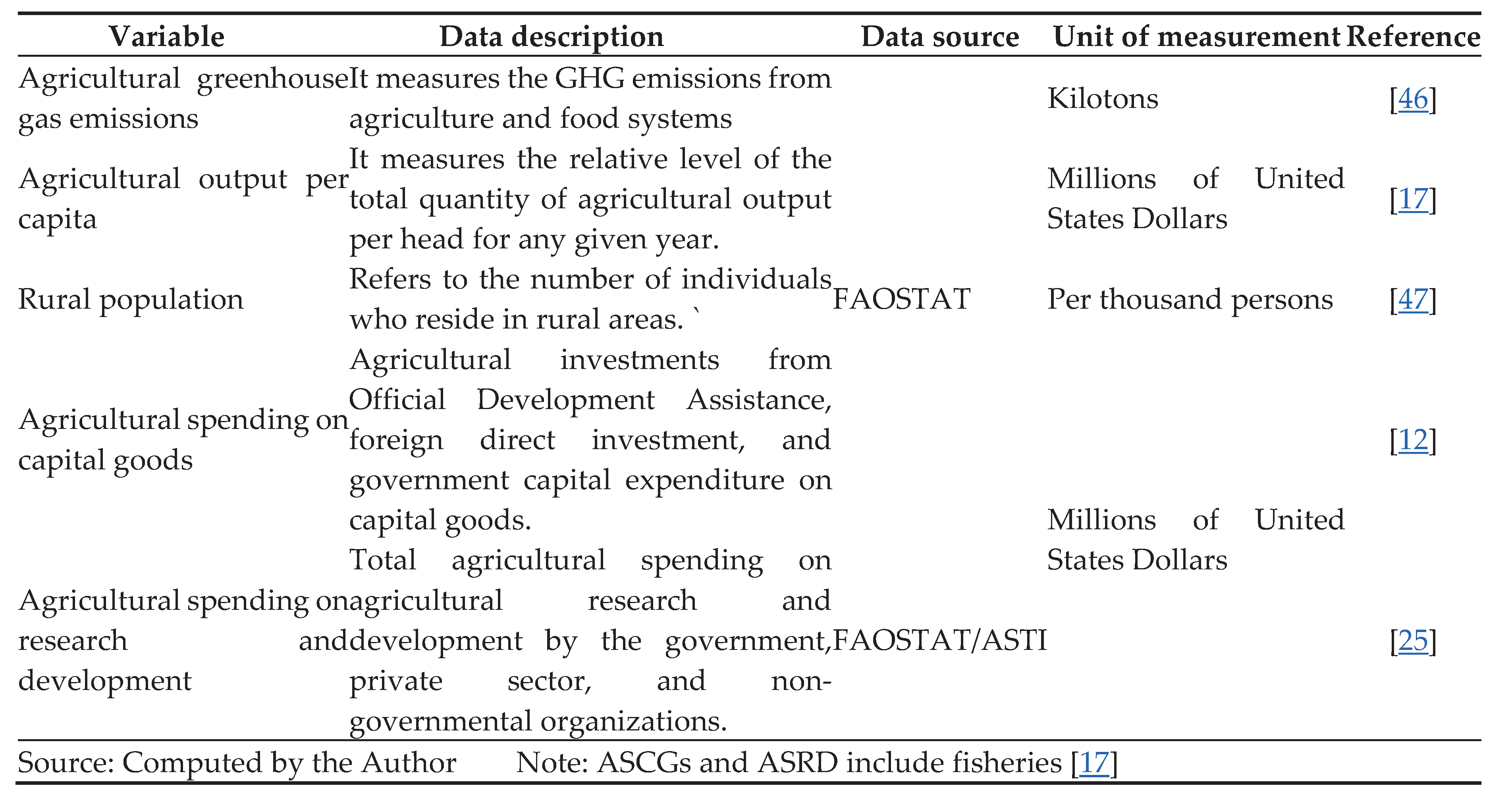 |
Table 2.
Descriptive analysis.
| Variables | Arab Maghreb Union | East African Community | Economic Community of West African States | South Africa Development Community |
Full Sample |
| Mean | Mean | Mean | Mean | Mean | |
|
(Standard deviation) |
(Standard deviation) |
(Standard deviation) |
(Standard deviation) |
(Standard deviation) | |
| Agricultural greenhouse gas emissions (In kilotons) |
187551.00 | 562248.50 | 256886.60 | 682709.70 | 422349.00 |
| (56650.75) | (123258.80) | (25115.27) | (60627.08) | (219903.90) | |
| Agricultural output per capita (In million US$) |
0.0799 | 0.0345 | 0.2168 | 0.4229 | 0.1885 |
| (0.0137) | (0.0018) | (0.0279) | (0.0285) | (0.1531) | |
| Rural population (per thousand people) | 30880.98 | 140938.00 | 154659.10 | 74527.09 | 100251.30 |
| (207.24) | (28945.87) | (22262.31) | (9650.04) | (53770.47) | |
| Agricultural spending on research and development (In million US$) | 1287.45 | 745.05 | 691.99 | 850.64 | 893.78 |
| (2092.44) | (2615.48) | (2312.95) | (609.68) | (2045.42) | |
| Agricultural spending on capital goods (In millions of US$) | 325.96 | 753.28 | 706.41 | 1527.72 | 828.34 |
| (213.39) | (631.62) | (569.09) | (2915.92) | (1565.70) |
Source: Computed by the Author.
Table 3.
Serial correlation, cross-sectional dependence, and panel unit root test results.
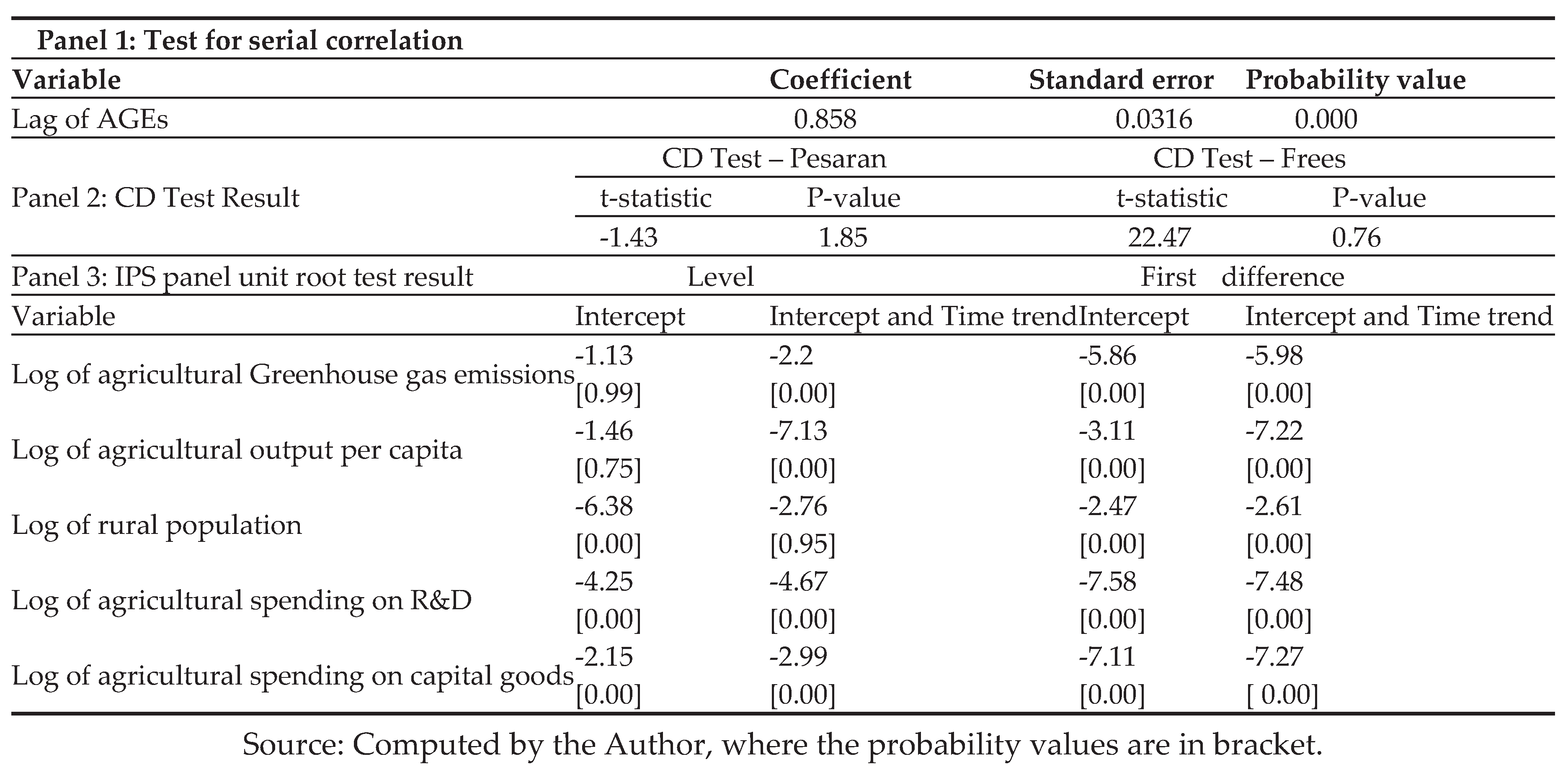 |
Table 4.
Co-integration test results.
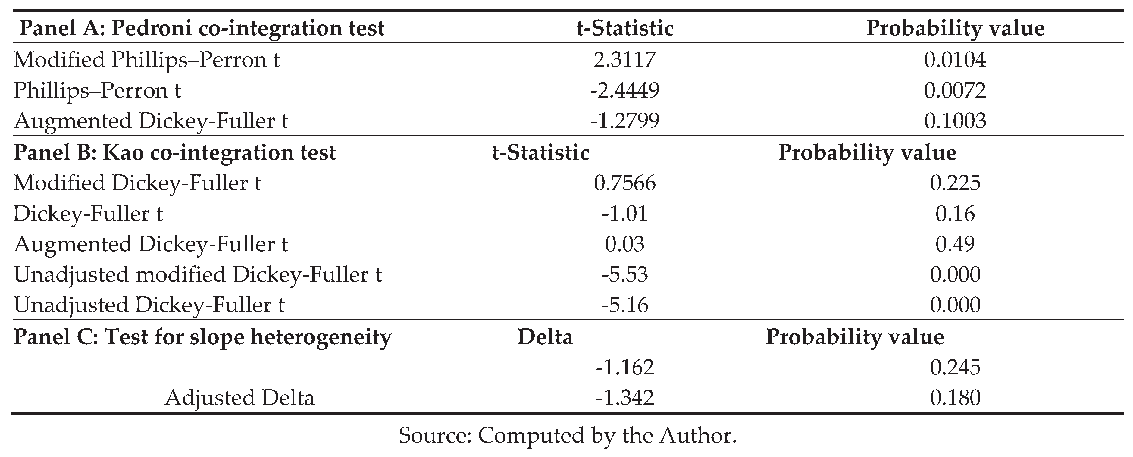 |
Table 5.
Fully Modified Ordinary Least Squares results.
|
Variable |
FMOLS | CCR | ||
| Elasticity coefficient | Proportional change in kt | Elasticity coefficient | Proportional change in kt | |
| Agricultural spending on capital goods | -0.04*** (0.0207) [-16.63] |
0.9996 |
-0.04*** (0.0286) [-12.56] |
0.9996 |
| Agricultural spending on research and development |
0.01 (0.0121) [1.9] |
1.0001 |
0.01 (0.0193) [1.4] |
1.0001 |
| Agricultural output per capita | 0.47*** (0.1631) [12.24] |
1.0046 |
0.5*** (0.2234) [9.57] |
1.0050 |
| Rural population | 1.11*** (0.3745) [ 47.96] |
1.0111 | 1.04*** (0.4069) [42.01] |
1.0104 |
Source: Estimated by the Author, where the parenthesis represents standard errors and bracket t-statistic. Kt means kiloton. NOTE: We consider a t-statistic that is less than 2 to be insignificant and those at 2 and above to be significant. The statistical significance of the variables is represented by three asterisks (***) symbolizing that they are statistically significant at most 5%.
Disclaimer/Publisher’s Note: The statements, opinions and data contained in all publications are solely those of the individual author(s) and contributor(s) and not of MDPI and/or the editor(s). MDPI and/or the editor(s) disclaim responsibility for any injury to people or property resulting from any ideas, methods, instructions or products referred to in the content. |
© 2025 by the authors. Licensee MDPI, Basel, Switzerland. This article is an open access article distributed under the terms and conditions of the Creative Commons Attribution (CC BY) license (http://creativecommons.org/licenses/by/4.0/).
Copyright: This open access article is published under a Creative Commons CC BY 4.0 license, which permit the free download, distribution, and reuse, provided that the author and preprint are cited in any reuse.


