
Submitted:
29 October 2023
Posted:
30 October 2023
You are already at the latest version
Abstract
Climate change not only affects weather conditions, patterns, and the frequency and severity of extreme weather events but also changes how governments spend money. Agriculture is an important sector of the European Union (EU), and it is projected to decrease by 16% by 2050, therefore a third of the EU budget has been spent on agricultural funding, adaptation, and climate action. The effect of climate change on agriculture is mixed and dependent on the country and its location. The southern EU is adversely affected while the northern EU is positively affected by the changes in weather patterns. The main goal of this paper is to gain insight regarding the effect that climate change has on public spending in relation to the agricultural sector of the EU, by using the pooled OLS and GMM methods. The study concluded that agriculture has a significant impact on public spending in the southern countries of the EU, where it represents a significant portion of the GDP. Inflation influences public spending in the whole EU region, the northern and southern countries of the EU. Rain has a moderately significant impact on public spending in the whole EU region. It is advised that governments maintain a controllable level of inflation using fiscal and monetary policy that will implicitly control public spending.
Keywords:
climate change
; public spending
; agriculture sector
; GMM
1. Introduction
Climate change is defined by the National Aeronautics and Space Administration as “a long-term change in the average weather patterns that have come to define Earth’s local, regional, and global climate” [1]. Climate change is associated with an increase in ozone level, air pollutants, temperature, rainfall, and snowfall in certain areas while in other areas there is an increase in droughts and water scarcity. Another effect that climate change has consists in the increase of sea and ocean levels, and increase in intensity, frequency and severity of hurricanes and wildfires [2]. To limit climate change and global warming, the Paris Agreement was established in 2015. The Paris Agreement is an international legal binding treaty between 193 parties that has the role of limiting global warming to 1.50-2.0 degree C compared to the pre-industrial levels and eliminating greenhouse gases [3]. According to the Intergovernmental Panel on Climate Change Report, global temperature is forecasted to increase by 1.3 to 2.4 °C in 2020-2060 and from 1.9 to 5.7 °C in 2061-2100, if pollution control policies and emissions control processes are not implemented [4]. The National Centers for Environmental Information reports that in 2021 the global warming temperature is situated at 1.04 degree C, compared to the pre-industrial levels [5].
Climate change affects fiscal sustainability and increases financial risk. The fiscal impact of climate change is due to the allocation function which is split into mitigation and allocation policies and redistribution and stabilization function. All functions have a direct impact that increases the expenditure side of the public budget and decreases the revenue side [6]. The direct costs associated with climate change are estimated to be 122 billion euro for a 3-degree Celsius increase scenario, mortality due to extreme heat, a median of 234 billion euro due to sea-level rise, 2.4 trillion euro in a high emission scenario and 21 billion euro due to river floods in a moderate scenario. The loss from extreme weather events is projected to range between 4 and 8 billion euro while the loss associated with the agricultural sector is projected to be 831 million euros and for arable production [7]. Climate change has a direct mixed effect on agriculture, depending on the country and its location. On one hand, in southern European countries, with an established warmer weather, climate change negatively impacts harvested agricultural output level, the consistency of it, and the level of production quality due to an increase in drought, heat stress, and lack of precipitation. Besides the negative effect on crops, the land exhibits a downgrade in quality and productivity [8]. On the other hand, in the northern European countries, where the climate is colder, climate change has a positive effect on agriculture due to an increase in temperature and a decrease of the cold and frost that extends the growing period [9].
The main component of the EU’s agricultural policy is the Common Agricultural Policy (CAP). In the EU, 54 billion euros of public funds were spent yearly under the CAP since 2006. Globally approximately 640 billion euros are spent as agricultural subsidies. During the period 2014- 2020, 38% of the EU’s budget is allocated to CAP which equals a total of 362.8 billion euros [10]. An audit regarding the efficiency of CAP shows that the funds are misallocated, increase income disparity, and increase the land value which only benefits landowners, not farmers. A big proportion of funding is directed to countries that would be well-off in the absence of the payments. According to the report of the European Court of Auditors issued in 2022, during the years 2014-2020, climate spending has been overstated by 72 billion euros, 80% of which was allocated to agricultural funding. The results show that only 13% of the budget was spent on climate action [11]. As of 2021, in the EU, the estimated gross value added from the agricultural industry was 189.4 billion euros and contributed 1.3% to EU’s GDP [12]. Osberghaus & Reif [13] state that although the costs of agricultural adaptation due to climate change are high and most of them are private, by 2050, the agricultural sector of the European Union will decrease by 16%. 40% of EU’s land is categorized as agricultural land and it provides 22 million jobs within the agricultural sector and another 22 million jobs outside of the sector.
Because of climate change, governments need to increase public spending due to disaster relief payments and infrastructure rebuilding. Climate change has an impact on other economic sectors, such as labor and tourism [14], [15], therefore, climate change reduces the tax base and adversely affects fiscal balance. Droughts, rising temperatures, and extreme weather conditions have a negative effect on the agricultural and tourism sector which implicitly lowers GDP. As a result, the countries' fiscal budgets will fall due to a decrease in the amount of income generated by the government, and an increase in government expenditures due to adaptation costs. There are also indirect consequences that consist in devaluation of other sectors due to job and income loss [15].
Europe experiences weak precipitations and higher temperatures. Such conditions do not only the impact the agricultural sector by decreasing the crop quality and yield, but also the energetic sector that experiences lower generation of hydropower and challenges associated with maintaining the cooling systems in power plants. According to the GDO Analytical Report created by the European Commission titled “Drought in Europe”, the August 2022 edition, the Combined Drought Indicator states that 17% of Europe is in alert conditions while 47% is under warning conditions (As shown in Figure 1). Although the drought hazard has increased in Italy, Spain, Portugal, France, Germany, Netherlands, Belgium, Luxembourg, Romania, Hungary, Serbia, Ukraine, Moldova, Ireland and the United Kingdom, the countries that are experiencing severe conditions are Italy, France, Hungary, and Romania. According to the Standardized Precipitation Index, a severe to extreme drought is experienced in Italy, France, and Eastern Europe [16].
The originality and novelty of this paper is that it adds insight into the relationship between public spending and climate change by looking at new variables such as agriculture. Previous literature focused on using temperature and precipitation as proxy for climate change impact while this research is using agricultural output as proxy for climate change.
The present paper aims at a thorough examination of this relationship, starting from the following question: How does climate change affect public spending in relation to the agriculture sector?
The purpose of this paper is to show the effect of climate change on public spending by looking at the EU’s agricultural sector. With an increase in temperature due to global warming, a decrease in the agricultural sector is expected, which will increase public spending and affect the public budget by creating a deficit. Also, an increase in agricultural spending should support economic development, therefore a higher spending on the agricultural sector should increase GDP. The Generalized Method of Moments Analysis (GMM) methodology is applied to exhibit the implications of climate change on public spending in all EU countries, by using the following variables: harvested agriculture output, real GDP growth, inflation, debt-to-GDP ratio, greenhouse gas from agriculture, labor in the agricultural sector, temperature, and rain, during the 2000-2020 period.
2. Literature Review
According to Aaheim et al. [14] climate change has a direct impact on the agricultural sector due to the high dependence between agriculture and climatic factors. In Europe, agriculture contributes to GDP differently according to region. While in the Baltics and Central Europe East the value added is more than 15%, in other regions it is less than 10%. According to Yadav et. al. [17], climate change affects the agricultural sector in six different ways soil, crop production, water, temperature, CO2, pests, and diseases. Due to the increases in temperature and extreme weather conditions caused by climate change, the soil loses its moisture, starts to erode and, over time, exhibits infertility which negatively impacts the quality and quantity of crops. An increase of 10 degrees Celsius decreases agricultural harvest output by 1.7%, while a decrease of 100 millimeters in rainfall reduces agricultural growth by .35%. Although climate change has a direct impact on the agricultural sector, the agricultural sector also influences climate change through the emission of greenhouse gases. According to OECD [6], the agricultural sector emits greenhouse gases that contribute to climate change. The increase in the amount of greenhouse gasses impacts temperature and changes the pattern of precipitations. The constant change in environmental conditions has an adverse effect on the amount of output and quality generated from the agricultural sector and environment. Although, as far as the authors’ knowledge, there are no studies that are looking at the effect of climate change, proxied as agricultural output, on public spending there is a somewhat consensus regarding the effect of climate change, proxied as temperature and rain or extreme weather events, on public spending.
Lis & Nickel [18] looked at evidence taken from the occurrence of extreme weather events. Their results show that depending on the economic development level of the country, an extreme weather event decreases budget balance by 0.23% and GDP by 1.4%. The budget balance of developing countries is worse off after an extreme weather event compared to the budget balance of advanced economies. Parker [19] shows that the impact that extreme weather events have on countries are dependent on the level of economic development and the type of disaster. Boneva & Ferrucci [20] reveal that extreme weather events caused by climate change led to higher prices and monetary policy shocks that increase inflation. Also, financial tools used to off-set the negative effects of climate change, such as carbon tax, have a direct impact on inflation. According to Batten et. al. [21] events caused by climate change led to a decrease in GDP, decrease in financial gain and the supply of global commodities. A detailed analysis was conducted by Cannone [22] that states that globally there will be a short to medium-term inflation caused by the effect of climate change in the agricultural sector that will increase the prices on food and from the actions needed to mitigate the effect of it. The impact that extreme weather events have on public spending and budget balance is further explained by Bachner & Bednar-Friedl [23] using an analysis based on Austria. Due to the necessity of frequent relief payments and reconstruction of infrastructure, public spending increases creating an exacerbating imbalance in the public budget. Besides the effect on the expenditure side, revenue is also negatively affected through the reduction of the sectoral tax base, and lower revenues earned from taxes. Such simultaneous actions exacerbate the imbalance in the public budget. The exacerbated imbalance indirectly affects other sectors due to the low availability of funds that can be allocated to other sectors. The results show that without a counterbalancing method, the effect that climate change has on public budget is -.3% compared to the baseline. The revenue side is decreased by low labor tax revenue (-.4%) and low production revenue (-.8%), and the expenditure side increases due to disaster relief (+184%) and unemployment benefits (+10%). GDP and welfare are also lower compared to the baseline by -.2%, respectively -.6%, while unemployment is higher compared to the baseline by .4%.
Looking at the impact that climate change, proxied by temperature and rain, has on public spending and budget balance, the results do not reach a consensus regarding the impact each variable has on public spending. Giovanis & Ozdamar [24] reveal that temperature has a negative effect on the government’s budget and increases debt. The average temperature reduces budget balance by 0.3% and expands debt by 1.87%. The study has forecasted temperature and rain patterns for a period of 79 years and concluded that upholding present conditions will adversely affect the budget balance by 7.3% and increase the levels of debt by 16% in 2060–2079 and 18% in 2080–2099. Previous forecasts have been projected under a scenario of high level of greenhouse gases. Changing the forecasts to a scenario that is based on low level of greenhouse gases, budget balance decreases by 1.7% in 2020–2039 and 2.2% in 2080–2099, while the levels of debt increase by 5% in 2020–2039 and 6.3% in 2080–2099. Kahn et. al. [25] shows that increase in temperature decreases GDP growth in the short and medium run, which implicitly reduces the budget of governments. The impact of temperature depends on the level of economic development of each country, low-income countries being more affected compared to emerging economies. An increase of 1 degree Celsius from the median temperature of the emerging economies decreases growth by 0.9%, while an increase of 1 degree Celsius from the average temperature of low-income countries decreases growth by 1.2%. Kahn et. al [25] concluded that continuous changes in temperature, above and below the historical benchmark, adversely affect per capita growth. Another conclusion that has been reached in the same study is that changes in the pattern of precipitation do not have any effect on capita growth. The research shows that the impact of an increase in temperature is different according to geographic regions and income level. The analysis shows that an increase in temperature of 0.04 °C per year will decrease GDP by more than 7% by the year 2100, unless adaptation policies are put in place.
Although previous studies are showing that temperature increases debt, spending and decreases GDP growth, Leppänen et. al. [26], shows that in the cold climate of Russia, an increase in temperature decreases public spending by a small amount. The authors suggest that Russia can save up to $3-4 billion, during a period of 20 years, from 2000-2020, under an increase in temperature of 1-2 degree Celsius. If the increase in temperature is higher than 1-2 degree Celsius, there could be possible environmental consequences that are harder to predict due to data limitation. Therefore, the impact that temperature has on public spending could be dependent on the climate of the region. Yahaya [27] analysis based on ECOWAS countries, contradicts previous studies, and concludes that the only variable that negatively affects budget balance by creating a deficit is rainfall. The extreme changes in rainfall pattern reduce the amount of revenue generated and increase expenses. The following scenario will force countries to borrow more money and exacerbate public spending.
Climate change also causes inflation which implicitly affects public spending. According to a study conducted by Ezirim et. al. [28] there is an interdependence between inflation and public expenditure in the short run but also the long run. An increase in inflation will result in an increase in public spending and vice versa. Different results were obtained by George-Anokwuru & Ekpenyong [29] that found that the relationship between public expenditure and inflation is positive and insignificant in the short-run and negative and significant in the long-run. Due to an analysis conducted by Adediran et.al. [30] we can confirm that at a global level, climate change has an inflationary effect on the global economy due to the extreme weather events that disrupt supply chain which directly increases prices of food, by its effect on the labor efficiency and effectiveness, and increase in fuel prices and production costs.
3. Materials and Methods
This paper demonstrates the effect of climate change on public spending by looking at evidence from the agricultural sector. The Generalized Method of Moments Analysis (GMM) methodology is applied to establish climate change effects on public spending from the period 2000-2021, in all 27 EU countries which are Belgium, Bulgaria, Czechia, Denmark, Germany, Estonia, Ireland, Greece, Spain, France, Croatia, Italy, Cyprus, Latvia, Lithuania, Luxembourg, Hungary, Malta, Netherlands, Austria, Poland, Portugal, Romania, Slovenia, Slovakia, Finland and Sweden. The paper also analyzes the effect of climate change on public spending in the Northern and Southern countries of Europe. The countries were grouped in Northern and Southern according to the United Nations. The northern countries are Ireland, Denmark, Lithuania, Estonia, Finland, Sweden, and Latvia, while the southern countries are Spain, Italy, Greece, Croatia, Malta, Portugal, and Slovenia. The reason for dividing the countries according to the region is because climate change affects the northern and southern part differently, while the conditions in the southern part of EU are worsening for the agriculture sector, the conditions in the northern countries of EU are facilitating the agricultural sector.
The research design of this paper follows the GMM model proposed by Yahaya [27] which concludes that the only variables that have an impact on public spending are rainfall and previous years’ deficit. Besides the variables used in the previously stated study such as GDP growth, inflation, temperature, debt-to-GDP ratio, and rainfall, this study adds new variables. The new variables added to this study are harvested agricultural output as a percentage of GDP, greenhouse gas emitted by the agricultural sector, and employment in the agricultural sector. We are using the harvested agricultural output as a percentage of GDP and employment in the agricultural sector to assess the impact the agricultural sector has on public spending. Data regarding greenhouse gas emissions from the agricultural sector is used to assess climate change and the impact that greenhouse gases have on public spending. Compared to the study conducted by Yahaya [27] the new variables added to our study are meant to provide evidence on the impact that climate change has on public spending by looking at the agricultural sector of the EU, Northern EU countries and Southern EU countries. Our model is using public spending as an independent variable and harvested agricultural output, GDP growth rate, inflation rate, debt-to-GDP ratio, greenhouse gas from agriculture, agricultural labor, mean temperature deviation and rainfall as dependent variables.
Table 1 presents the variables used in our model, abbreviations, unit, and data source used to gain insight about the relation between public spending, climate change and agriculture.
The effect that climate change has on public spending by looking at the agricultural sector has been analyzed by looking at the following model:
(1) SPD𝑖, 𝑡 = 𝛽0 ± 𝛽1 AGR𝑖, 𝑡± 𝛽2 GHG𝑖, 𝑡 ± 𝛽3 ΔDTG𝑖𝑡 ± 𝛽4 GDP_GR𝑖, 𝑡 ± 𝛽5 𝐼NF, 𝑡± 𝛽6 LAB𝑖, 𝑡 ±𝛽7 TEMP𝑖, 𝑡 ±𝛽8 RAIN𝑖, 𝑡± 𝛿𝑡 ± 𝛾𝑡 ± 𝜇𝑖, 𝑡
In the regression equation, SPD is the dependent variable followed by the independent variables AGR𝑖, 𝑡, GHG𝑖, 𝑡, INF𝑖, 𝑡, DTG𝑖𝑡, GDP_GR𝑖, 𝑡, LAB𝑖, 𝑡, TEMP𝑖, 𝑡, RAIN𝑖, 𝑡. 𝑖 represents each country within the data set, while 𝑡 represents different time periods. 𝛽 are each variable’s coefficients while 𝛿, 𝛾, 𝜇 represent error terms.
The reason for choosing harvested agricultural output is that it is dependent on weather conditions. It is also regarded as the major occupation of individuals [34]. Agriculture has a direct effect on GDP because it provides direct and indirect job opportunities and facilitates economic development, which is the reason why we choose labor in the agricultural sector. Therefore, the variable we choose to use in our study is harvested agricultural output as a percentage of GDP. The GDP growth rate is the annual average increase in GDP based on the market prices using the local currencies. To assess the fiscal policy of each country we used the variable debt-to-GDP ratio which gives us a better perspective about each country’s ability to pay its debt created by public spending. While a lower debt-to-GDP ratio shows a better budget balance, a higher rate increases interest payments, unbalancing the public budget [35]. Public spending is how governments manage to achieve their objectives and differs according to the size of the country [36]. We choose greenhouse gases from the agricultural sector as a way of assessing climate change. The reason for using temperature and rain as variables is to gain a better perspective of the change in environmental conditions, and because the agricultural sector is dependent on these two factors.
This research adopts panel data analysis techniques because it is the best fit for our data. Our data is a blend of time cross-sections section data that is observed at multiple time periods. The model used in this statistical analysis takes into consideration unobservable heterogeneity within the dataset that accounts for bias and unobserved variables providing accurate results. The analysis uses instrumental variables to account for endogeneity issues [37]. Thus, we adopted a system estimator that uses adjusted standard errors to account for possible heteroskedasticity issues within the dataset [38]. The following method accounts for unobserved effects by using GMM’s instrumental variables to fix any issues related to endogeneity [39]. The next section presents the empirical results of this study and what the effects the independent variables have on the dependent variable.
From a statistical perspective, Table 2 lists the key descriptors of the variables employed in all the EU27 countries.
From Table 2, we notice that the highest standard deviation is for the variable harvested agricultural output (14956.29), which shows that heterogeneity is present within the dataset. The large standard deviation shows us that the values within the dataset are farther from the mean (10190.58), which can pose a problem to our analysis due to high frequency of extreme values. The second largest standard deviation is for the variable labor in the agricultural sector (578.65). The smallest standard deviation is for the variable inflation which has a value of 3.302, showing that the values within the variables are closer to the mean ( -2.503) and the dataset does not present high variability. The second smallest standard deviation is for the variable GDP (3.872). It is noticeable that all variables have 567 observations, besides labor in the agricultural sector which has 562 observations, and greenhouse gas which has 324 observations. Looking at the scatterplot in Figure 2 we obtain insight about the relationship between public spending and the other variables in all EU.
Table 3 lists the key descriptors of the variables employed in South EU countries.
Table 3 shows the descriptive statistics from the Southern and Northern region of EU. Harvested agricultural output has a high standard deviation in both regions, 8670.115 in the South and 2641.584 in North. In the Southern region labor from the agricultural sector also has the highest standard deviation of 431.67, while in the Northern region rain has the second highest standard deviation of 2641.584. The variables that have the lowest standard deviation in the Southern region are greenhouse gas from the agricultural sector and inflation with the values .657982, respectively 1.752775, while in the Northern region the variables with the lowest standard deviation are inflation and temperature with a value of 2.338374, respectively 2.57159. The large difference in standard deviation could pose a problem to the analysis due to the high variability within the data set and lack of consistency. Looking at the scatterplot in Figure 3 and Figure 4 we obtain insight about the relationship between public spending and the other variables in the northern and southern part of EU.
Table 4 shows the correlation matrix for all the European Union countries.
Table 5 presents the correlation matrix of the countries in the southern region of the European Union.
Table 6 presents the correlation matrix of the countries in the northern region of the European Union.
Table 4, Table 5 and Table 6 show the correlation matrixes of the whole EU region, the southern part, and the northern part of EU. In the whole EU region, the variables that have the highest correlation regarding public spending are greenhouse gases, labor in the agricultural sector and temperature. In the southern region of EU, the variables that are significantly correlated to public spending are agriculture and labor in the agricultural sector. In the northern part of EU, no variable is significantly correlated to public spending.
4. Results
Four modeling approaches have been employed in this study's statistical analysis: pooled ordinary least square (Pooled OLS), random effects model (REM), fixed effects model (FEM), and Generalized moments of methods (GMM). These approaches are most frequently used in the related analysis of this kind of panel data. Taking into consideration that each model had its own limitations, the least square model (FGLS) and panel-corrected standard errors model (PCSE) has been used in the case of all 27 EU countries, 7 Northern countries from EU and 7 Southern countries of EU.
For all 27 European countries the analysis started with a pooled OLS regression using the data from 2000-2020. On the sampled data, the Breusch-Pagan/ Cook-Weinsberg and White test was used which resulted in a p-value of .1297, respectively 0.000. Therefore, the OLS model is suitable but the data shows signs of heteroskedasticity. The multicollinearity test using the variance inflation factors averages all variables at 1.35 with no values above 5, therefore there is no multicollinearity within the dataset. Using the Breusch and Pagan Lagrangian test to assess the random effects within the panel shows a p-value of 0.000 which means that it is appropriate to use REM over OLS within the sample. REM proves a random variation within countries, and the unobserved variables are uncorrelated with the independent ones. The Hausman test was used on the data set to assess the better fit between REM and FEM. The p-value concluded that REM is better fitted due to 0.0562 > 0.05. The data was also tested using the Wooldridge and Pesaran test, which both resulted in a p-value of 0.000 <0.05 respectively 0.333, therefore within the panel data there are signs of autocorrelation and cross-dependence. Ramsey RESET test for robustness show 0.0226> 0.05. To correct the previous issues, the panel-corrected standard errors (PCSE) were used due to having the number of observations higher compared to periods of time. We notice that for all European countries in the pooled OLS model, rain and inflation had a significant effect on public spending, although the REM model adds agriculture and labor in agriculture as influencing public spending. The PCSE correction only shows that inflation, greenhouse gas, and rain are significant while the GMM model shows that all the variables, besides GDP, are significant. The common variables that are perceived to have a significant impact on public spending are inflation and rain.
The same analysis was used on the southern and northern part of the European Union, although the results are different. Looking at the southern part of the European Union, collinearity has been found within the dataset therefore the variables labor in agriculture and temperature have been dropped. The Breusch Pagan/ Cook-Weinsberg test had p- values of 0.0311, respectively 0.7040 which are > than 0.05 therefore the OLS model is suited for the analysis and there is no sign of heteroskedasticity. The results of the Hausman test are 0.2864 which means that REM is suitable for the analysis. The Wooldridge test for autocorrelation resulted in a value of 0.0260, showing that there is no autocorrelation within the variables. However, the Pesaran test 0.376 that means cross-dependence, is not present. Ramsey RESET test for robustness show 0.9847> 0.05. The results for the pooled OLS show that inflation, agriculture, and greenhouse gasses influence public spending the most, while the FEM model shows that inflation, agriculture, and rain have a substantial impact. The GMM model shows that all variables, besides GDP, have a strong impact on public spending. In the northern part of EU, the Breusch- Pagan and White test has resulted in a p-value of 0.0004, respectively 0.0107, therefore the OLS model is suited and data shows signs of heteroskedasticity. The VIF test used for multicollinearity identified that there is multicollinearity for the greenhouse variable, therefore dropped it and we ended up with a mean of 1.72. Using the Breusch and Pagan Lagrangian test to assess the random effects within the panel shows a p-value of 1.000 which shows that the OLS model is suitable for the analysis. The Hausman test resulted in a p-value of 0.000, which means that FEM is suitable for this analysis. The Breusch- Pagan LM show 0.0756, Wald show 0.0000, Wooldridge has a p-value of 0.0010 and the Pesaran test has a value of 0.373, meaning that the data is not presents signs of autocorrelation, cross-sectional dependence and heteroskedasticity. To correct these data related to the fit-panel data model (FGLS) was used more time periods than the number of observations. Ramsey RESET test for robustness show 0.9847> 0.05. After, the GMM model was used, which omitted the variable temperature. For the pooled OLS analysis, the variables that have a significant impact on public spending are inflation and rain, while the FEM model identifies that inflation, agriculture, labor from agriculture, temperature and rain have a significant impact on public spending. The FGLS model shows that only inflation has a significant effect on public spending. GMM analysis has omitted the variable temperature and shows that all variables, but GDP, strongly influence public spending.
Table 7 represents the Pooled OLS and GMM analysis of the statistical significance that the variables GDP, inflation, debt-to-GDP, harvested agricultural output, greenhouse gases from the agricultural sector, labor in the agricultural sector, temperature and rain have on public spending.
From Table 7 we notice that the variable that has the highest impact on public spending is inflation. Also, rain has a moderate and significant impact on public spending. In the southern part of EU countries, agriculture has a moderate impact on public spending, while in the northern EU countries, the relationship between variables is missing. In some cases, looking at the whole EU region we can state that temperature has a significant impact on public spending. On the other hand, we cannot state that GDP has an impact on public spending.
4. Discussion
From the previous analysis we have reached the same conclusions as previous articles, that rain and temperature have a negative impact on GDP in all EU countries. Therefore, the increase in the two variables will implicitly decrease GDP. In all EU there is a positive relationship between temperature and harvested agricultural output, which shows that the increase in temperature will increase agricultural output. In the Southern region of EU there is a negative relationship between rain and GDP and a positive relation between labor in the agricultural sector and public spending.
The results of this study support the research conducted by Yahaya [27]. Our study also suggests that temperature impacts public spending in the whole EU region. The mutual conclusion reached is that inflation is positively affecting public spending across the whole EU regions and the northern and southern countries of the EU. Although our study has similar results as Yahaya [27], we could not prove that GDP has a positive effect on public spending, while rain only has a moderate significance on public spending in the whole EU region.
Looking at the southern parts of the EU the results that have been obtained are correlated with previous studies of Aaheim et.al.[14]. In the southern part of the EU, agriculture is the main contributor to GDP. Due to the lack of precipitation and increase in drought periods, the agricultural output is expected to decrease. In our study, we have found that for the southern part of the EU, the variables that have a significant influence on public spending are inflation, harvested agricultural output and greenhouse gases. Because of the heavy reliance of south Europe on the agricultural sector, any variable affecting the agricultural sector has a direct effect on public spending. Our study also concludes the same hypothesis as Ahmed et.al.[40], which is that there is a positive relationship between the agricultural sector and public spending.
In the northern part of EU, inflation has a significant impact on public spending. Harvested agricultural output also has an impact on public spending but it is not as significant due to the low reliance, low development of the agricultural sector and its small contribution to GDP. The northern part of EU does not have the favorable climate needed for the expansion of the agricultural sector, although the conditions might change due to environmental warming.
The study conducted has its own limitations. One of the limitations consists in the availability of data. Data used to analyze greenhouse gases is only available between the years 2009-2020, although all the analysis was conducted with data from 2000-2020, therefore the results could be biased. Another limitation is using the GMM model that assumes that the data has a Gaussian distribution, which could result in a misrepresentation of the data. There is also the presence of multicollinearity which forced us to drop certain variables. Because we had multicollinearity in our analysis it is possible that our variables are correlated. If the variables are correlated, then it becomes difficult to accurately predict the relation between variables. In our GMM analysis, a couple of variables have been omitted in the results by the model. We believe that this happened due to multicollinearity, although the variables that have been exhibiting multicollinearity have dropped.
A third limitation would be the amount of data available. Although our study was conducted over a period of 20 years, the methodology can use a larger time frame to better understand the effect variables have on public spending. We recommend that further research will either use a larger time frame or a different econometric model to study the impact that climate change has on public spending by looking at the agricultural output in the EU countries.
5. Conclusions and policy implications
Climate change is one of the most important issues of our century, and it threatens not only the agricultural sector, the weather, economic conditions but our whole existence. Looking at the effect that climate change has on public spending using evidence from the agricultural sector, most research articles refer to underdeveloped countries such as Nigeria, Mexico, Ethiopia, Ghana, Uganda, and Tanzania, but there are no studies, as far as we know, that are looking at developed countries.
The main findings of our research show that inflation has a significant effect on public spending within the European Union and the northern and southern parts of the European Union. Agriculture affects public spending in regions where it contributes significantly to GDP, such as the southern countries of the EU. In regions in which agriculture is not a main sector, for example the northern part, inflation is the only variable that influences public spending. The increase in public spending adversely affects each countries’ budget balance without an offsetting increase in budget revenues. Therefore, countries with a large amount of public spending may run into the risk of having high sustained inflation which can slow down the growth of a country and increase the inequality within the population.
The southern part of the European Union is in worse condition compared to the northern part. In the southern part the increase in droughts will affect the fertility and quality of the soil, creating harsh agricultural conditions and desertification. On the other hand, the agricultural sector will start playing a major role in the northern part of the European Union. The migration of the population is also inevitable in these conditions; therefore, migration might become a future issue.
As far the policy implication goes, we recommend that governments use fiscal policy to control the level of inflation in their country that will implicitly control public spending. An effective strategy would be for governments to create a monetary and fiscal policy aiming to reduce inflation. Monetary policy can focus on increasing the interest rates to decrease the money supply and decrease demand that will result in lower inflation. Also, an increase in each country’s production efficiency will create downward pressure on the prices of goods produced within the country that will implicitly reduce inflation. The fiscal policy tools that can be used to reduce inflation will be an increase in tax rate, and price caps for goods and wages. By using the previous fiscal policy tools, the demand and spending will be reduced which will lower the rate of inflation.
The findings of the study have significant policy implications for addressing the economic effects of climate change on public spending in the EU agricultural sector. Policymakers should adopt a multi-faceted approach to tackle these challenges. Firstly, effective measures to control inflation should be implemented through appropriate monetary policies to maintain price stability and safeguard public spending. Secondly, targeted support should be provided to the agricultural sector, particularly in regions where it plays a significant role in GDP, such as the southern countries of the EU. This support should focus on promoting sustainable practices and enhancing resilience to climate change. Additionally, policymakers need to prioritize climate change adaptation by investing in irrigation systems and encouraging crop diversification to mitigate the adverse impacts on agricultural output and public spending. It is essential to strike a balance between public spending and budget revenues, emphasizing fiscal discipline and exploring revenue generation avenues. Furthermore, policymakers must consider long-term planning, regional disparities, and potential migration challenges, to ensure sustainable development and effectively address the impacts of climate change on public spending.
In addition to these recommendations, policymakers have a crucial role in addressing the specific needs and vulnerabilities of small countries in the face of climate change. A targeted policy framework should be developed that recognizes the unique challenges faced by these nations, such as limited resources and capacity constraints. Furthermore, ensuring equitable distribution of resources is essential, necessitating a greater allocation of funding and support to poorer countries compared to wealthier ones. By implementing a policy that prioritizes assistance to vulnerable nations and promotes inclusive and sustainable development, policymakers can foster resilience, reduce inequality, and create a more balanced and just response to the impacts of climate change across different countries and regions.
Author Contributions
Conceptualization, G.D.; methodology, I.C.N and A.E-N.; software, I.C.N., and A.E-N.; validation, G.D; I.C.N and A. E-N.; formal analysis, G.D., and I.C.N.; investigation, I.C.N.; resources, I.C.N. and A.E-N.; data curation, A.E-N.; writing—original draft preparation, I.C.N., and A.E-N.; writing—review and editing, G.D.; I.C.N.; visualization, G.D.; supervision, G.D.; project administration, G.D., and I.C.N. All authors have read and agreed to the published version of the manuscript.
Funding
This research received no external funding.
Institutional Review Board Statement
Not applicable
Informed Consent Statement
Not applicable.
Acknowledgments
Not applicable.
Conflicts of Interest
The authors declare no conflict of interest.
References
- National Aeronautics and Space Administration. Weather, Global Warming and Climate Change. Available online: https://climate.nasa.gov/global-warming-vs-climate-change/ (accessed on 15 October 2022).
- Congressional Budget Office. Budgetary effects of climate change and of potential legislative responses to it. Available online: https://www.cbo.gov/publication/57175#_idTextAnchor003 (accessed on 10 Novemeber 2022).
- United Nations. The Paris Agreement United Nations. Available online: https://www.un.org/en/climatechange/paris-agreement#:~:text=Today%2C%20193%20Parties%20(192%20countries,strengthen%20their%20commitments%20over%20time (accessed on 9 Novemeber 2022).
- IPCC, A.R6.; climate change: the physical science basis. The Working Group I contribution to the Sixth Assessment Report, Intergovernmental Panel on Climate Change. 2021.
- NCEI. Assessing the global climate. Available online: https://www.ncei.noaa.gov/news/global-climate-202112 (accessed on 22 November 2022).
- OECD.Climate Change and Long-Term Fiscal Sustainability. OECD. Available online: https://www.oecd.org/gov/budgeting/scoping-paper-on-fiscal-sustainability-and-climate-change.pdf. (accessed on 20 October 2022).
- United Nations Office for Disaster Risk Reduction. Available online: https://www.preventionweb.net/publication/climate-change-impacts-eu-new-evidence-recent-research (accessed on 21 October 2022).
- Agovino, M.; Casaccia, M.; Ciommi, M.; Ferrara, M.; Marchesano, K. Agriculture, climate change and sustainability: The case of EU-28. ELSEVIER 2019, Volume 105, page range 525–543.
- Scown, M. W.; Brady, M. V.; Nicholas, K. A. Billions in misspent EU agricultural subsidies could support the Sustainable Development Goals. One Earth 2020, Volume 3, page range 237–250. [CrossRef]
- European Court of Auditors. Special report - climate spending in the 2014-2020 EU budget. Available online: https://www.eca.europa.eu/Lists/ECADocuments/SR22_09/SR_Climate-mainstreaming_EN.pdf (accessed on 22 November 2022).
- European Commission. Performance of the agricultural sector. Performance of agricultural sector - Products Eurostat News – Eurostat. Available online: https://ec.europa.eu/eurostat/web/products-eurostat-news/-/ddn-20210413-2 (accessed on 10 December 2022).
- Osberghaus, D.; Reif, C. Total costs and budgetary effects of adaptation to climate change: An assessment for the European Union. SSRN Electronic Journal. 2010, page range 1-46.
- Aaheim. A; Amundsen. H; Dokken. T; Wei, T. Impacts, and adaptation to climate change in European economics. Global Environ Chang 2012, Volume 22, page range 959-968.
- European Commission. Climate impacts in Europe- The JRC PESETA II Project. Available online: https://publications.jrc.ec.europa.eu/repository/handle/JRC87011 (accessed on 13 December 2022).
- European commission. Drought in Europe august. Available online: https://edo.jrc.ec.europa.eu/documents/news/GDO-EDODroughtNews202208_Europe.pdf (accessed on 15 December 2022).
- Yadav, D.; Gupta, A.; Gupta, P.; Ranjan, S.; Gupta, V.; Badhai, S. Effects of Climate Change on Agriculture. Researchgate 2020.
- Lis, EM.; Nickel, C. The impact of extreme weather events on budget balances, International Tax and Public Finance journal 2010, Volume 17, Page range 378-399. [CrossRef]
- Parker, M. The impact of disasters on inflation. Economics of Disasters and Climate Change journal 2017, Volume 2, Page range 21–48.
- Boneva, L.; Ferrucci, G. Inflation and climate change: The role of climate variables in inflation forecasting and macro modelling. Inspire 2022.
- Batten, S.; Sowerbutts, R.; Tanaka, M. Climate change: Macroeconomic impact and implications for monetary policy. Ecological, Societal, and Technological Risks and the Financial Sector 2020, page range 13-38.
- Cannone, E. (2022, October 24). The role of climate change on inflation forecasting using time varying parameters model. Master’s Degree Thesis, Luiss Guido Carli University, Italy, 26 Jan 2023.
- Bachner, G.; Bednar-Friedl, B. The effects of Climate change impacts on public budget and implications of fiscal counterbalancing instruments, Environmental Modeling & Assessment 2019, Volume 24, page range 121- 142. [CrossRef]
- Giovanis, E.; Ozdamar, O. The impact of climate change on budget balances and debt in the Middle East and North Africa (MENA) region. Climatic Change journal 2020, Volume 172, page range (3-4). [CrossRef]
- Kahn ME.; Mohaddes K.; Ng RN; Pesaran MH; Raissi M; Yang JC. Long- term macroeconomic effects of climate change: a cross- country analysis, Energy Economics 2021, Volume 104. [CrossRef]
- Leppänen S; Solanko, L.; Kosanen, R. The impact of climate change on regional government expenditure: evidence from Russia, Environ Resources Econ 2017, Volume 67, page range 67-92. [CrossRef]
- Yahaya, B.; Nkwatoh, S.; Louis; Jaere. A.; Babagana. Impact of Climate Change on Budget Balance: Implications for Fiscal Policy in the ECOWAS Region, International Journal of Economics and Finance 2021, volume 13.
- Ezirim, C.; Muoghalu, M.; Elike, U. Inflation versus public expenditure growth in the U.S.: An empirical investigation. North American Journal of Finance and Banking Research 2010, Volume 2.
- George-Anokwuru, C. C.; Ekpenyong, B. I. Government expenditure and inflation in Nigeria. Journal of Economics and Management Sciences. 2020, Volume 3. [CrossRef]
- Adediran, I. A.; Isah, K. O.; Ogbonna, A. E.; Badmus, S. K. A global analysis of the Macroeconomic Effects of Climate Change. Asian Economics Letters. 2023. [CrossRef]
- Database – Eurostat. Available online: https://ec.europa.eu/eurostat/data/database (accessed on 15 December 2022).
- The World Bank.Databank. Available online: https://databank.worldbank.org/metadataglossary/world-development-indicators/series/GC.NLD.TOTL.GD.ZS. (accessed on 25 November 2022).
- World Bank Climate Change Knowledge Portal. Home. Available online: https://climateknowledgeportal.worldbank.org/ (accessed on 23 December 2022).
- Kapur, Radhlka. Significance of Agriculture and food production, University of Delhi, ResearchGate. 2020.
- Ortiz-Ospina, E.; Roser, M. Government spending. Our World in Data. Available online: https://ourworldindata.org/government-spending?fbclid=IwAR1AbgbCrF2wlfYZPJYFQHjSab3ougHy19Bzts4QuEWitKjs4oIi0n6ChWc (accessed on 30 November 2022).
- Tujula, M. and Wolswijk, G. What determines fiscal balances? An empirical investigation in determinants of changes in OECD budget balances. European Central Bank, Working Paper Series No. 422 / December 2004, Frankfurt am Main, Germany.
- Wooldridge, J. M. Econometric Analysis of Cross Section and Panel Data. Cambridge, M.A: MIT. 2002.
- Arellano, M.; Bond, S. Dynamic Panel Estimation Using DPD98 for GAUSS: A Guide for Users. Working Paper, Institute for Fiscal Studies. 1998. Available online: http://www.cemfi.es/~arellano/#dpd.
- Chuku, C. The Proposed Eco: Should West Africa Proceed with a Common Currency? Paper presented at the Centre for the Study of African Economies (CSAE) 2012 Conference on “Economic Development in Africa”, Oxford University, Oxford. 2012, 18-20.
- Ahmed, T.; Khan, K. S.; Naeem, M. The effect of public spending on agricultural growth: Evidence from 1972 to 2014 in Pakistan. Sarhad Journal of Agriculture 2019, Volume 35. [CrossRef]
Figure 1.
Drought map source: European Drought Observatory.
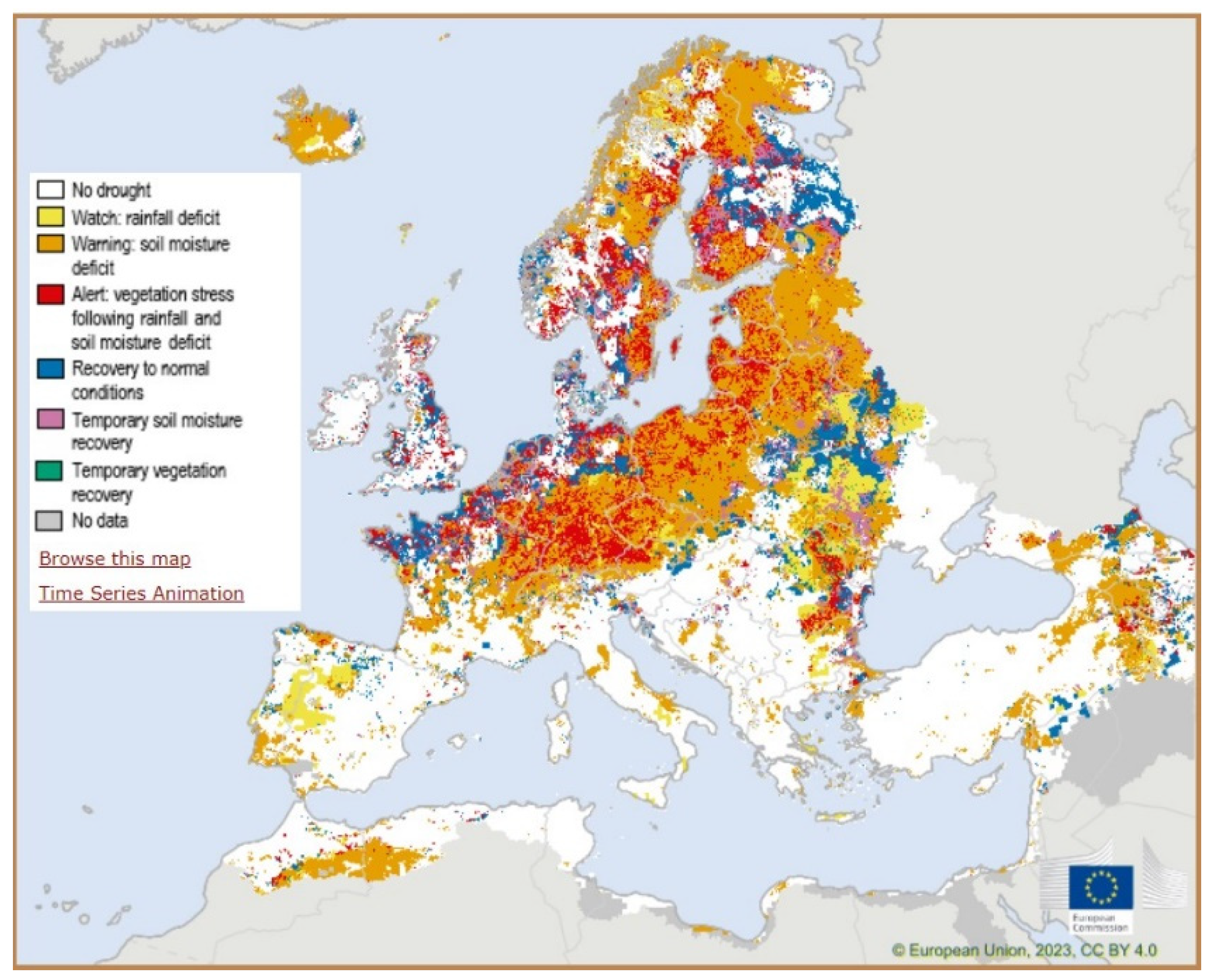
Figure 2.
Scatter plot of SPD and each variable; All EU.
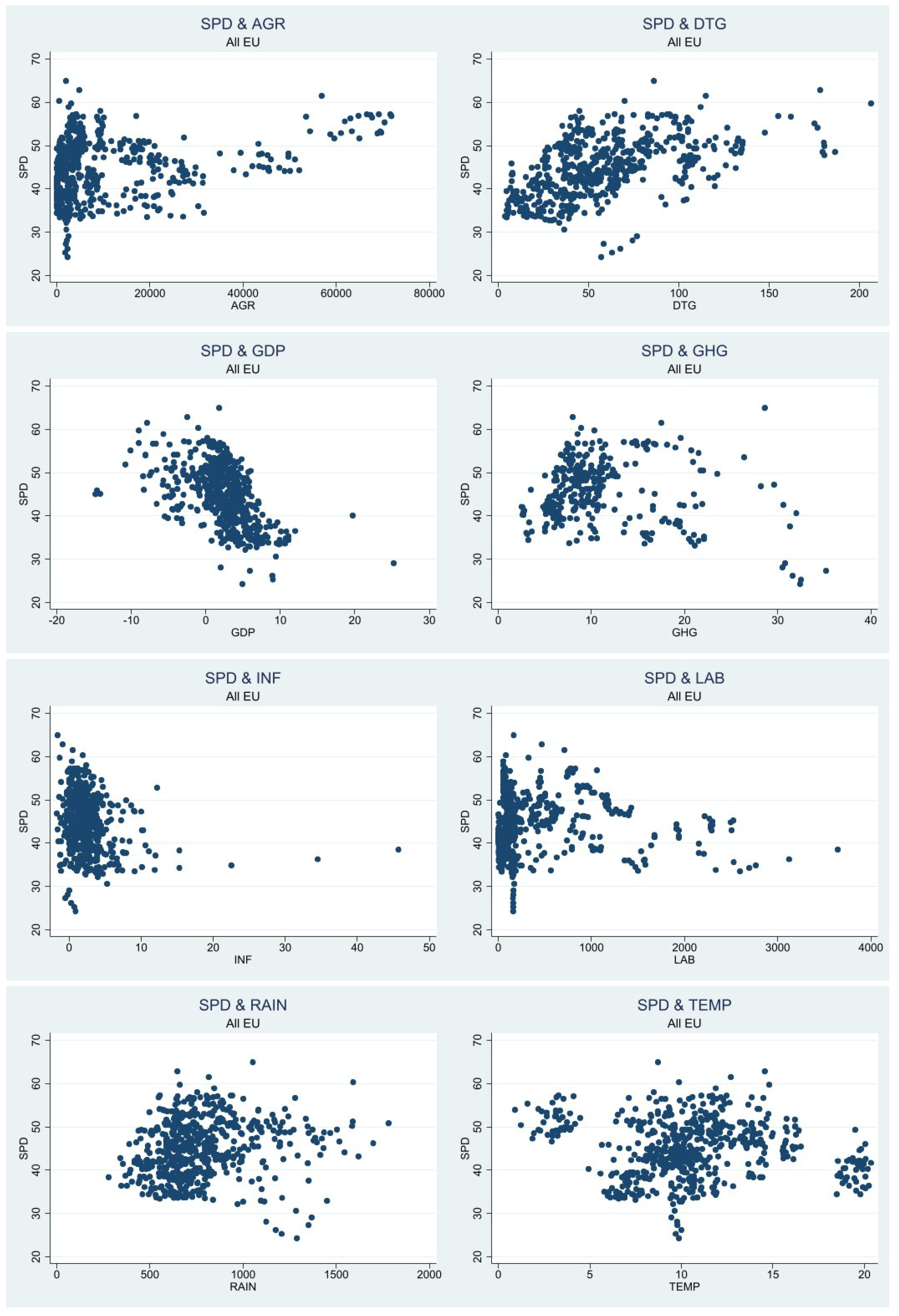
Figure 3.
Scatter plot of SPD and each variable; North EU.
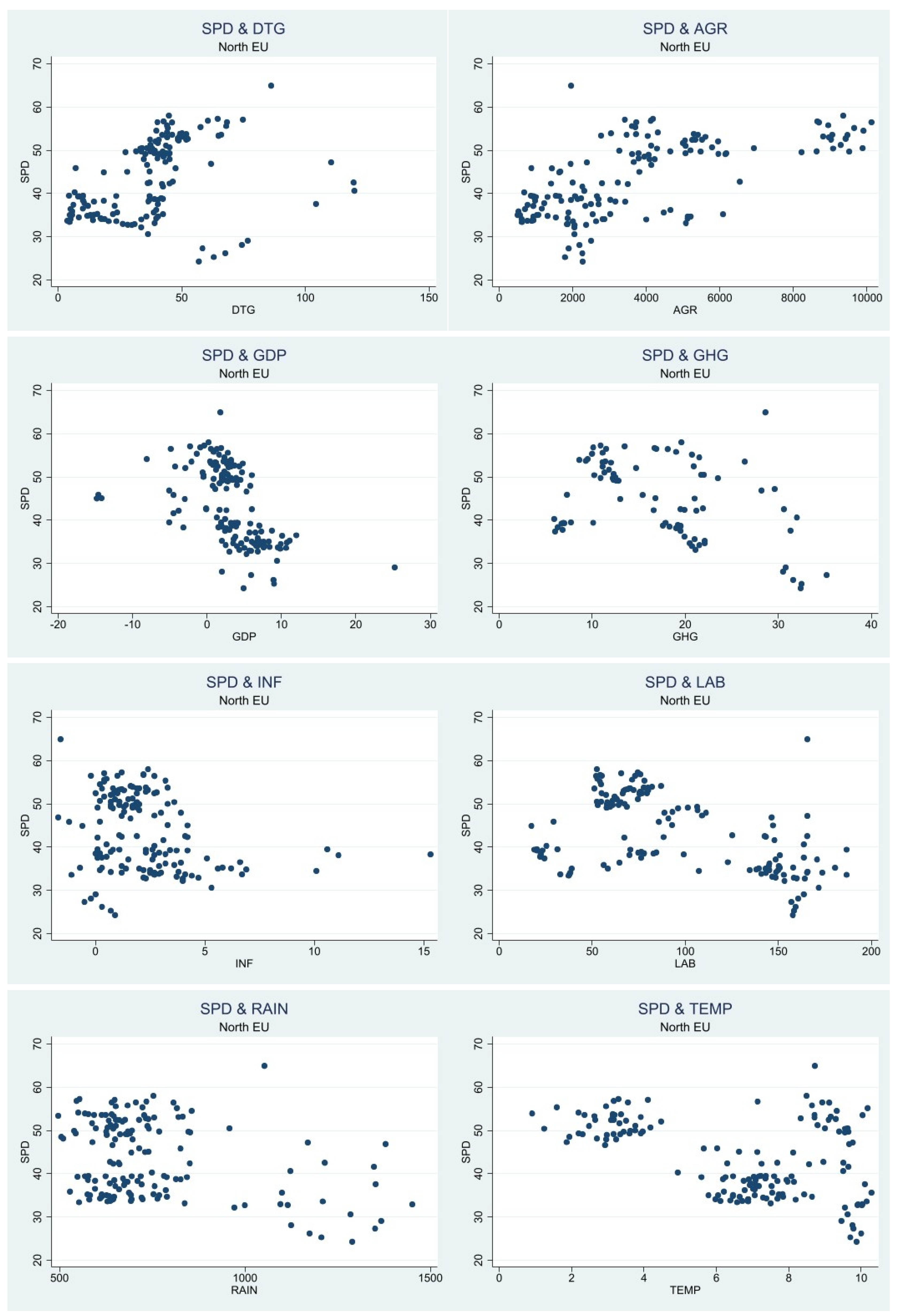
Figure 4.
Scatter plot of SPD and each variable; South EU.
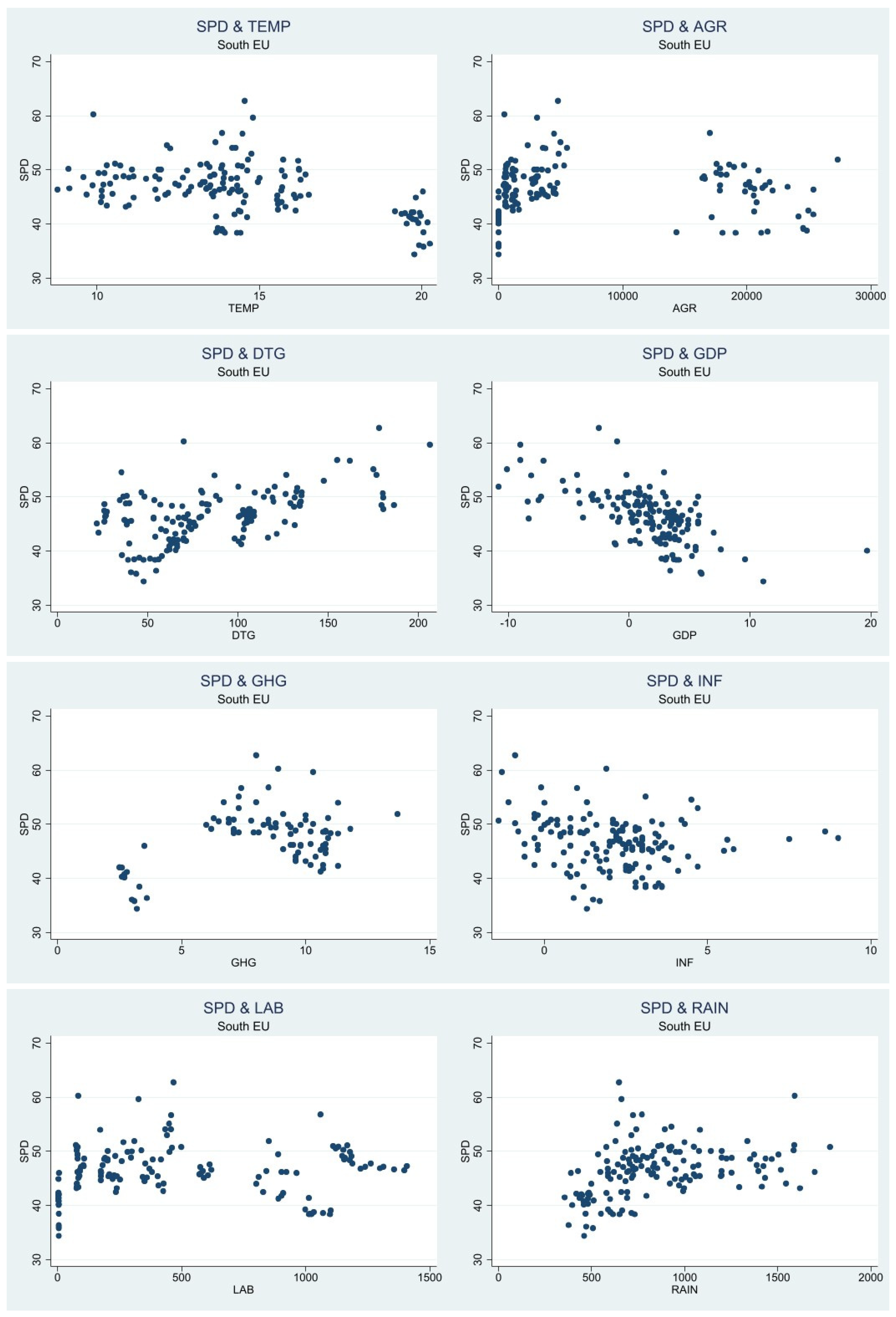

Table 1.
Variables, abbreviation, unit, source.
| Variables Name | Abbreviation | Unit | Source |
| Dependent Variables | |||
| Public Spending | SPD | %GDP | Eurostat 2000-2020 [31] |
| Independent Variables | |||
| Harvested agricultural output | AGR | %GDP | Eurostat 2000-2020 [31] |
| GDP growth rate | GDP_GR | %Annual | World Bank 2000-2020 [32] |
| Inflation Rate | INF | %Average Consumer Price | Eurostat 2000-2020 [31] |
| Debt-to-GDP ratio | DTG | %GDP | Eurostat 2000-2020 [31] |
| Greenhouse Gas from Agriculture | GHG | % Agriculture | Eurostat 2009-2020 [31] |
| Agricultural labor input statistics | LAB | Absolute figures | Eurostat 2000-2020 [31] |
| Mean temperature deviation | TEMP | %Annual | Climate Change Knowledge Portal 2000-2020 [33] |
| Rainfall | RAIN | %Annual | Climate Change Knowledge Portal 2000-2020[33] |
Source: Adapted from Yahaya et al. [27].
Table 2.
Descriptive statistics EU27 countries.
| Variable | Observations | Mean | Std. dev | Min | Max |
|---|---|---|---|---|---|
| SPD | 567 | 44.9 | 6.6 | 24.3 | 64.9 |
| GDP | 567 | 2.2 | 3.8 | -14.8 | 25.2 |
| INF | 567 | 2.5 | 3.3 | -1.7 | 45.7 |
| DTG | 567 | 58.8 | 34.9 | 3.8 | 206.3 |
| AGR | 567 | 10190.5 | 14956.2 | 0 | 71870.7 |
| GHG | 324 | 10.8 | 6.0 | 2.5 | 35.2 |
| LAB | 562 | 405.9 | 578.6 | 3.34 | 3645 |
| TEMP | 567 | 10.6 | 3.8 | .91 | 20.35 |
| RAIN | 567 | 781.7 | 242.0 | 278.4 | 1780.0 |
Source: processed by authors.
Table 3.
Descriptive statistics of South and North EU countries.
| South EU countries | North EU countries | |||||||||
|---|---|---|---|---|---|---|---|---|---|---|
| Variable | Obs. | Mean | Std. dev | Min | Max | Obs. | Mean | Std. dev | Min | Max |
| SPD | 147 | 46.4 | 4.7 | 34.4 | 62.8 | 147 | 43.5 | 8.7 | 24.3 | 64.9 |
| GDP | 147 | 1.3 | 4.0 | -10.8 | 19.7 | 147 | 2.9 | 4.7 | -14.8 | 25.2 |
| INF | 147 | 2.0 | 1.7 | -1.4 | 9 | 147 | 2.1 | 2.3 | -1.7 | 15.3 |
| DTG | 147 | 85.9 | 41.4 | 21.8 | 206.3 | 147 | 37.6 | 21.9 | 3.8 | 119.9 |
| AGR | 147 | 7114.6 | 8670.1 | 0 | 27329.4 | 147 | 3826.7 | 2641.5 | 505.7 | 10116.8 |
| GHG | 84 | 8.3 | 2.6 | 2.5 | 13.7 | 84 | 17.3 | 7.6 | 5.9 | 35.2 |
| LAB | 142 | 474.4 | 431.6 | 4.0 | 1408.5 | 147 | 94.1 | 47.3 | 17.2 | 186.7 |
| TEMP | 147 | 14.2 | 2.9 | 8.7 | 20.2 | 147 | 6.5 | 2.5 | .91 | 10.2 |
| RAIN | 147 | 858.1 | 328.1 | 355.3 | 1780.0 | 147 | 753.4 | 209.2 | 496.4 | 1451.2 |
Table 4.
Correlation Matrix EU27.
| SPD | GDP | INF | DTG | AGR | GHG | LAB | TEMP | RAIN | |
|---|---|---|---|---|---|---|---|---|---|
| SPD | 1.0000 | ||||||||
| GDP | -0.5058 | 1.0000 | |||||||
| INF | -0.2208 | 0.1620 | 1.0000 | ||||||
| DTG | 0.5136 | -0.3363 | -0.2743 | 1.0000 | |||||
| AGR | 0.2504 | -0.0940* | -0.0274*** | 0.1648 | 1.0000 | ||||
| GHG | -0.1372* | 0.1112* | -0.1267* | -0.0812*** | 0.0570*** | 1.0000 | |||
| LAB | -0.0663*** | -0.0308*** | 0.3798 | 0.0834* | 0.5237 | -0.0016*** | 1.0000 | ||
| TEMP | -0.1041* | -0.0665*** | -0.0476*** | 0.4418 | 0.0230*** | -0.3069 | 0.0843* | 1.0000 | |
| RAIN | 0.1556 | -0.0549*** | -0.1095* | 0.0749** | -0.1038* | 0.2392 | -0.1851 | -0.1485 | 1.0000 |
Note: *, ** and *** denote significance at 1%, 5% and 10% respectively. Source: processed by authors
Table 5.
Correlation Matrix Southern EU.
| SPD | GDP | INF | DTG | AGR | GHG | LAB | TEMP | RAIN | |
|---|---|---|---|---|---|---|---|---|---|
| SPD | 1.0000 | ||||||||
| GDP | -0.6222 | 1.0000 | |||||||
| INF | -0.2144 | 0.2602 | 1.0000 | ||||||
| DTG | 0.5153 | -0.4216 | -0.5111 | 1.0000 | |||||
| AGR | -0.0423*** | -0.1530** | -0.0.781*** | 0.2085* | 1.0000 | ||||
| GHG | 0.3764 | -0.3108 | -0.2336* | 0.1435*** | 0.2018** | 1.0000 | |||
| LAB | 0.0976*** | -0.1594** | -0.0328*** | 0.3475 | 0.9193 | 0.1295 | 1.0000 | ||
| TEMP | -0.4411 | 0.1191*** | -0.1786* | 0.1443** | -0.1393** | -0.6833 | -0.1757* | 1.0000 | |
| RAIN | 0.3542 | -0.0605*** | 0.0562*** | -0.2440 | -0.2647 | 0.4827 | -0.2570 | -0.7640 | 1.0000 |
Note: *, ** and *** denote significance at 1%, 5% and 10% respectively. Source: processed by authors.
Table 6.
Correlation Matrix Northern EU.
| SPD | GDP | INF | DTG | AGR | GHG | LAB | TEMP | RAIN | |
|---|---|---|---|---|---|---|---|---|---|
| SPD | 1.0000 | ||||||||
| GDP | -0.5019 | 1.0000 | |||||||
| INF | -0.2710 | 0.1157*** | 1.0000 | ||||||
| DTG | 0.3715 | -0.1612** | -0.4514 | 1.0000 | |||||
| AGR | 0.6402 | -0.2507 | -0.2647 | 0.2724 | 1.0000 | ||||
| GHG | -0.3846 | 0.2295* | -0.3701 | 0.6077 | 0.1357*** | 1.0000 | |||
| LAB | -0.4770 | 0.2810 | 0.0094*** | 0.2750 | -0.2310 | 0.7871 | 1.0000 | ||
| TEMP | -0.4463 | 0.1257*** | 0.0368*** | -0.0106*** | 0.0779*** | 0.7499 | 0.3389 | 1.0000 | |
| RAIN | -0.3441 | 0.1336*** | -0.0703*** | 0.3749 | -0.1285*** | 0.7556 | 0.4691 | 0.5817 | 1.0000 |
Note: *, ** and *** denote significance at 1%, 5% and 10% respectively. Source: processed by authors.
Table 7.
p-values showing the statistical significance of the considered variables.
| Dependent variable SPD | |||||||||||||||
|---|---|---|---|---|---|---|---|---|---|---|---|---|---|---|---|
| Independent variable | Pooled OLS | REM | FEM | PCSE | GMM | ||||||||||
| EU27 | South EU | North EU | EU 27 | South EU | North EU | EU27 | South EU | North EU | EU 27 | South EU | North Eu | EU 27 | South EU | North EU | |
| GDP | -.5641 (.0637) |
-.6264 (.0705) |
-.4945 (.0955) |
-.5366 (.0402) |
-.6264 (.0705) |
-.4945 (.0955) |
-.5416 (.0399) |
-.6664 (.0769) |
-.4783 (.0877) |
-.3371 (.0562) |
-.5742 (.0658) |
-.3317 (.1114) |
-.6505 (.0236) |
-1.1340* (.2749) |
-.4381* (.1391) |
| INF | -.0400*** (.1872) |
-.2823*** (.2492) |
-.2799*** (.3716) |
-.2066** (.1237) |
-.2823*** (.2492) |
-.2799*** (.3716) |
-.2775* .1253) |
-.5435* (.2637) |
-.6228** (.3528) |
-.2951* (.1317) |
-.3315*** .2702) |
-.3769*** (.3201) |
.0513*** (.0327) |
-1.0066*** (1.8377) |
.7182*** (.9106) |
| DTG | .1073 (.0082) |
.0484 (.0103) |
.2524 (.0327) |
.0859 (.0130) |
.0484 (.0103) |
.2524 (.0327) |
.0869 (.0152) |
.0797 (.0272) |
.2219 (.0431) |
.1129 (.0137) |
.0522 (.0122) |
.2348 (.0560) |
.0152*** (.0182) |
-.3347*** (.4388) |
-.3721*** (.2802) |
| AGR | .0001 (.0000) |
-.0001*** (.0001) |
.0017 (.0002) |
.0007*** (.0000) |
-.0001*** (.0001) |
.0017 (.0002) |
.0000*** (.0000) |
.0000*** (.0002) |
-.0004*** (.0006) |
.0001 (.0000) |
-.0001** (.0000) |
.0015 (.0002) |
-.0001*** (.0001) |
.0091*** (.0095) |
.0020*** (.0018) |
| GHG | -.2533 .0456) |
-.3322** (.1691) |
-.6374* (.2402) |
-.4619 (.1055) |
-.3322* (.1691) |
-.6374 (.2402) |
-.9373 (.1829) |
-1.6096* (.6035) |
-1.0695 (.3305) |
-.2043*** (.1300) |
-.3317** (.1894) |
-.4192*** (.2804) |
.2051*** (.1034) |
0 (omitted) (0 omitted) |
0 (omitted) (0 omitted) |
| LAB | -.0036 (.0006) |
.0024*** (.0024) |
-.0609 (.0220) |
-.0012*** (.0014) |
.0024*** (.0024) |
-.0609 (.0220) |
.0003*** (.0023) |
.0125*** (.0106) |
-.1551*** (.0931) |
-.0029 (.0000) |
.0016*** (.0020) |
-.0666 (.0244) |
-.0070*** (.0044) |
-.1131*** (.1441) |
-.8194*** (.4383) |
| TEMP | -.7664 (.0777) |
-.8174 (.2320) |
-.2309*** (.3914) |
-.6675 (.1741) |
-.8174 (.2320) |
-.2309*** (.3914) |
.0228*** (.3138) |
-.7844*** (.8407) |
-.5025*** (.8559) |
-.7193 (.1009) |
-.9124 (.2766) |
-.4365*** (.42271) |
.0699*** (.2221) |
0 (omitted) (0 omitted) |
0 (omitted) (0 omitted) |
| RAIN | .0017*** (.0010) |
.0011*** (.0017) |
.0017*** (.0037) |
.0006922*** (.0014) |
.0011*** (.0017) |
.0017*** (.0037) |
.0010*** (.0015) |
.0007*** (.0020) |
-.0008*** (.0055) |
-.0009*** (.0011) |
.0004*** (.0017) |
-.0037*** (.0039) |
.0005*** (.0006) |
-.0040*** (.0108) |
-.0095*** (.0107) |
| _CONS | 48.6684 (1.4199) |
56.6611 (5.6550) |
44.0071 (2.6406) |
52.1868 (2.8117) |
56.6611 (5.6550) |
44.0071 (2.6406) |
49.5743 (3.9057) |
58.3822 (13.7217) |
74.0673 (12.3473) |
49.8825 (2.1964) |
58.4897 (6.5592) |
48.0482 (3.2222) |
17.5065* (2.8800) |
0 (omitted) (0 omitted) |
0 (omitted) (0 omitted) |
| OBS | 324 | 84 | 84 | 324 | 84 | 84 | 324 | 84 | 84 | 324 | 84 | 84 | 324 | 84 | 84 |
| PROP | 0.0000 | 0.0000 | 0.0000 | 0.0000 | 0.0000 | 0.0000 | 0.0000 | 0.0000 | 0.0000 | 0.0000 | 0.0000 | 0.0000 | 0.000 | 0.000 | 0.029 |
| R-SQUARED | 0.5906 | 0.7948 | 0.8063 | 0.5174 | 0.7984 | 0.8063 | 0.2145 | 0.3167 | 0.3533 | 0.8389 | 0.8208 | 0.8023 | |||
| F- STATISTIC | 56.79 | 37.13 | 39.03 | Wald chi2= 255.43 | 297.04 | 312.27 | 30.22 | 11.01 | 10.49 | Wald chi2= 223.75 | Wald chi2= 294.54 | 330.97 | 381.87 | 99.03 | 5.17 |
| SARGAN TEST | 0.012 | 0.246 | 0.366 | ||||||||||||
| Hansen test | 0.128 | 1.000 | 0.531 | ||||||||||||
Note: *, ** and *** denote significance at 1%, 5% and 10% respectively. Source: processed by authors.
Disclaimer/Publisher’s Note: The statements, opinions and data contained in all publications are solely those of the individual author(s) and contributor(s) and not of MDPI and/or the editor(s). MDPI and/or the editor(s) disclaim responsibility for any injury to people or property resulting from any ideas, methods, instructions or products referred to in the content. |
© 2023 by the authors. Licensee MDPI, Basel, Switzerland. This article is an open access article distributed under the terms and conditions of the Creative Commons Attribution (CC BY) license (http://creativecommons.org/licenses/by/4.0/).
Copyright: This open access article is published under a Creative Commons CC BY 4.0 license, which permit the free download, distribution, and reuse, provided that the author and preprint are cited in any reuse.


