
Submitted:
28 November 2025
Posted:
02 December 2025
You are already at the latest version
Abstract
Ensuring the structural integrity of high-energy piping systems is a critical requirement for the safe operation of nuclear power plants. This paper presents the design, imple-mentation, and three-year operational validation of a novel three-dimensional dis-placement monitoring system installed on the Steam Generator Blowdown pipeline of the Krško Nuclear Power Plant. The system was developed to confirm plant operating procedures will not cause excess dynamic displacements during operation.
The measurement system configuration utilizes three non-collinear inductive dis-placement transducers (HBM WA/500 mm-L), mounted via miniature universal joints to a reference plate and to a defined observation point on the pipeline. The arrangement enables real-time monitoring of X, Y, and Z displacements within a spherical meas-urement volume of approximately 0.5 m. Data are continuously acquired by an HBM QuantumX MX840B amplifier and processed using CATMAN Easy-AP software through a fiber-optic communication link between the containment and control areas.
The system has operated continuously for more than three years under elevated tem-perature and radiation conditions, confirming its reliability and robustness. The corre-lation of measured displacements with process parameters such as flow rate, pressure, and temperature provides valuable insight into transient events and contributes to predictive maintenance strategies. The presented methodology demonstrates a practical and radiation-tolerant approach for continuous structural monitoring of nuclear plant piping systems.
Keywords:
nuclear power plant
; piping systems
; displacement monitoring
; inductive transducers
; data acquisition
; radiation environment
; structural integrity
; experimental diagnostics
1. Introduction
At the Krško Nuclear Power Plant (NPP Krsko), a specific technical challenge has persisted for several years—to prove that regular operator actions as well as unpredicted transients on Steam Generator Blowdown System (BD) will not generate excessive dynamic forces which would result in excessive pipe displacements. As in all high-energy piping systems, the BD system is supported by a combination of fixed and dynamic hangers. These supports accommodate thermal expansion while simultaneously mitigating transient dynamic loads. Ensuring the structural integrity of such piping demands considerable engineering effort to achieve adequate support that allows controlled movement, maintains overall stability, and prevents damage under both normal and off-normal operating conditions.
Support components are routinely subjected to visual inspection for signs of degradation or abnormal behavior. Figure 1 and Figure 2 show typical pipe support components – sway struts and variable spring. Because the BD piping is located within the containment building, such inspections can be performed only during scheduled refueling outages, which occur every 18 months. Entry into containment during power operation is strongly discouraged due to elevated temperature, humidity, and, most importantly, radiation levels.
Pipe displacement in power plants can arise from several interacting factors, each contributing to the overall dynamic behavior of the piping system:
Thermal Expansion and Contraction: Temperature variations within the piping system cause the material to expand or contract. As the temperature of the conveyed fluid or the surrounding environment increases, the pipe expands; conversely, it contracts when the temperature decreases. These cyclic thermal deformations can induce movement and additional stresses in the piping network, particularly at locations with constrained boundary conditions or insufficient flexibility.
Vibrations and Dynamic Loads: Operational equipment such as pumps, valves, turbines, and compressors generate vibrations and transient dynamic loads. These loads can be transmitted through the piping system, leading to displacements and localized stress concentrations. In adverse conditions, this excitation can even result in resonant vibrations, amplifying the mechanical response and accelerating fatigue or wear of the support components.
Pressure Fluctuations: Rapid pressure changes can also induce significant pipe movements. Pressure surges, water hammer events, or abrupt variations in flow rate produce hydraulic forces that can push or pull the piping beyond its expected limits if the system is not adequately supported or damped.
Seismic Events: For power plants located in seismically active regions, ground motion due to earthquakes represents a major source of dynamic excitation. Seismic loading can induce substantial pipe displacements and impose additional stresses on supports and connecting elements. Proper seismic qualification of supports and structural anchorage is therefore essential to mitigate these effects and to ensure system integrity during seismic events.
To identify under which operating conditions that occurs - and to quantify the actual pipe displacements during plant operation, a dedicated monitoring system for displacement measurement was designed and implemented.
The principal objectives in developing the measurement system were as follows:
- to enable precise, real-time measurement of displacements in all three spatial directions (X, Y, Z),
- to ensure automatic data acquisition and archiving with subsequent analytical capability, and
- to provide continuous access to measurement data without requiring physical entry into the containment building.
The primary challenge was to develop a robust and reliable methodology for measurement, data acquisition, and processing suitable for industrial application under elevated temperature, humidity, and radiation conditions. To the best of the authors’ knowledge, this represents the first implementation of such a measurement approach within a nuclear power plant environment—and the first of its kind applied at the NPP Krško.
2. Materials and Methods
Due to its best reliability, linearity and rigidity, special in nuclear applications [2], a linear variable differential transformer (LVDT) was choosen as the basic element of the measurement chain. Inductive displacement transducers manufactured by Hottinger Baldwin Messtechnik (HBM), type WA/500mm-L. Displacement transducers of the WA-L series with a loose plunger design provide impressively reliable and highly precise measurement results. This type of sensor features a remarkably compact design (in relation to the measuring range). The compact dimensions of the sensor result from an active quarter-bridge circuit based on the differential inductor principle. The bridge is also integrated within the sensor, forming a full-bridge circuit that allows for easy connection of the WA-L transducer to the measuring amplifier. Insensitive to dirt, WA-L displacement transducers feature rugged mechanics and highly stable temperature behavior. This means they can be used in almost all industrial applications, delivering outstanding performance in displacement measurements (HBM, WA-L Displacement Transducers).
Inductive displacement transducers are generally designed to measure displacement along a single direction (the sensor axis). However, in our case, the movement of the observed point on the pipeline follows a spatial trajectory. Theoretically, if the position of the reference point on a reference plane were known, it would be possible to measure the position of the observed point on the pipeline using a single inductive displacement transducer. Such a transducer would need to be flexibly attached on one side to the reference point and on the other side to the observed point that moves. However, in this case, measuring only the change in distance would not be sufficient. To uniquely determine the position of the observed point, it would also be necessary to measure two angles: the angle between the perpendicular projection of the transducer axis onto the reference plane and the transducer axis itself, and the angle between the chosen coordinate axis in the reference plane and the projection of the transducer axis onto that plane [3].
Since continuous real-time measurement of these angles is impractical, we opted to determine the position of the observed point by simultaneously measuring three mutually non-collinear displacements using three inductive displacement transducers. These transducers are rotatably mounted on one side to the reference plane at three points with known coordinates, and on the other side, also rotatably attached to the observed point.
At the same time, it is necessary to consider that the measurements are carried out in a highly radioactive environment, which cannot be accessed during reactor operation. Therefore, the measuring system should not fail under any circumstances, meaning that a sufficiently large operating range must be provided. The system must be robust and capable of delivering reliable results for all theoretically possible positions of the observed points during the operation of the nuclear power plant. Consequently, we first defined the theoretically possible positions of the points in space in the form of a sphere and three cones, which define the volumes within which no obstacles may be present, ensuring the unobstructed operation of the measuring system (Figure 3).
Based on this, we also defined the measuring range of the individual components of the measurement system. For each observation point, the system consists of three inductive displacement transducers, which are attached on one side to a steel plate - representing the reference plane - using miniature universal (cardan) joints. The plate is mounted vertically so that it is parallel to the straight section of the pipe on which the point being monitored is located. The attachment points of the inductive transducers on the steel plate are arranged at the vertices of an equilateral triangle (Points T1, T2 and T3 in Figure 3).
At the other end, the inductive displacement transducers are attached to the pipe at the observation point P. The attachment to the pipe is achieved using a special clamp that allows the transducers to be positioned so that, in the initial position, their axes intersect as precisely as possible at point P on the pipe surface. On this side, the transducers are also mounted using identical miniature universal (cardan) joints.
When point P moves to point P’, the inductive transducers measure three non-collinear displacement values for each measuring point. From these, all three displacement components can be determined in the chosen coordinate system (see Figure 4, Figure 5 and Figure 6). The coordinate system is always defined such that the x-axis lies along the line connecting points T1 and T2; the y-axis is perpendicular to the x-axis within the plane defined by points T1, T2 and T3; and the z-axis is oriented perpendicular to the plane defined by the x and y-axes, forming a right-handed coordinate system.
The displacement components of point P, denoted as ux, uy and uz, are aligned parallel to the respective coordinate axes (see Figure 4).
Since the origin of the coordinate system is placed at point T_1, based on Figure 4 we can write equations (1), (2), and (3), which represent a system of equations from which the expressions for the coordinates of the point P(x_P, y_P, z_P) can be determined:
From the difference between equations (1) and (2), we obtain:
From the difference between equations (2) and (3), we obtain:
After substituting equation (4) into equation (5), we obtain:
From equation (1), we express :
Since points , , and are arranged in the reference plane in the form of an equilateral triangle with side length , the following relationships can be substituted into equations (4), (5) and (6): , and :
When point is displaced to point , the distances , , and change accordingly. These changes in distance can be expressed in the form:
Where , , and represent the values measured by the inductive displacement transducers during the movement of point to point . The values of the individual displacement components of point can be expressed as:
Measurements are performed at two locations. The first location is situated beneath the ceiling on the northern side of reactor building and is marked with the capital letter in Figure 7. The position of the measurement system and the orientation of the local coordinate system are shown in Figure 5.
The pipe displacement values at location are obtained by substituting the parameters , , and into equations (12), (13) and (14). Since the signal from the inductive displacement transducers, which measure the changes in distances , and , is negative when the length increases, the values , in in equations (12), (13), and (14) are replaced by , and , respectively.
In this way, the resulting expressions can be entered into the CATMAN Easy - AP software tool, which uses the measured three non-collinear displacements to calculate, in real time, the three displacement components of the selected point on the pipe within the coordinate system :
In the present case, the values measured during the installation of the system at position are substituted into equations (15), (16) and (17):
The second location is marked with the capital letter . The position of the measurement system and the orientation of the local coordinate system at this point are shown in Figure 6.
The pipe displacement values at location are obtained by substituting the parameters , , and into equations (12), (13) and (14). The values , in in equations (12), (13) and (14) are replaced by , in , respectively. The resulting expressions can then be entered into the CATMAN Easy - AP software tool for the real time calculation of the three displacement components of the point within the coordinate system :
In the present case, the values measured during the installation of the system at position are substituted into equations (21), (22) and (23):
Accuracy of the Measurement System
The accuracy of the designed measurement system was also examined. Since the inductive displacement transducers are mounted on both ends using miniature universal (cardan) joints, which exhibit a clearance between 0.1 mm and 0.2 mm, this factor alone introduces a measurement uncertainty on the order of approximately 0.5 mm.
An additional source of measurement error arises from the geometry of the system. It is technically impossible to attach all three inductive transducers to exactly the same point on the pipe - where the observed point is defined - using universal joints for each sensor. As shown in Figure 8, the attachment points of all three transducers on the pipe are therefore offset by 30 mm from the observed point. For small displacements, the geometric error of the system is practically negligible. However, as the displacement magnitude increases, this error becomes more significant. For large displacements - when the observed point reaches the extreme limits of the measurement range (±250 mm – Figure 3), particularly in directions parallel to the reference plane - the error can reach up to approximately 3 mm.
Figure 9.
Mounting of the inductive displacement transducers on the pipe at the observation point Q.
Figure 9.
Mounting of the inductive displacement transducers on the pipe at the observation point Q.
At first glance, this might suggest that the overall accuracy of the measurement system is relatively low. However, it should be emphasized that the primary objective was not to develop a high-precision laboratory instrument, but rather a robust measurement system with a large operational range (theoretically corresponding to a spherical volume with a radius of 250 – 300 mm). The system was designed to operate reliably under harsh environmental conditions while still providing dependable information about both the magnitude and direction of pipe displacements, with an accuracy fully sufficient for monitoring pipeline behavior under all operating regimes.
If higher accuracy were required, the same principle of measuring three non-collinear displacements could be retained, while replacing the inductive displacement transducers with three Posiwire encoder-based sensors (manufactured by ASM). In such a configuration, the free ends of the three measuring wires could be attached to the same point on the pipe being monitored, thereby eliminating the geometric offset that is inherent in the current design. However, this alternative arrangement would introduce a new challenge: due to the size and specific geometry of the sensors, it would be extremely difficult to ensure smooth winding and unwinding of the measuring wires in multiple displacement directions. The implementation of a fully rotatable mounting system for all three sensors would therefore be technically very complex.
Data Acquisition
As previously mentioned, the observation points and , whose displacements are monitored by the described measuring system, are located inside the reactor building, which cannot be accessed during reactor operation (Figure 7).
This means that inside the reactor building there are inductive displacement transducers with their supporting structures and a measuring amplifier, whose functions include supplying power to the sensors, data acquisition, amplification, filtering, and conversion of analog signals into digital ones. These digital signals are then transmitted to a personal computer located outside the reactor building, in the plant’s process computer room.
Due to the large distance between the measuring amplifier and the personal computer, communication between them takes place via an existing optical fiber cable, which is otherwise used for communication between the interior of the reactor building and the control room. Therefore, inside the reactor building, next to the measuring amplifier, an Ethernet-to-optical signal converter is installed, while outside, in front of the personal computer, an optical-to-Ethernet signal converter is installed.
Figure 10 shows the layout of the entire measurement system, Figure 11 shows data acquisition unit used, and Figure 12 shows a small cabinet, where the universal measurement amplifier HBM QuantumX MX840B (Figure 11) is located, together with ethernet to optical converters and power supplies. A CATMAN Easy - AP software, running on a personal computer, deals with daq unit communication, recalculating measuring results and archiving all the data in real time. Software application also allows more complex analysis (like FFT etc.), graphical representation and data export. For monitoring unusual spurious displacements, caused by system transients or seismic activity plain time domain graphs are used.
Measurement Configuration
Before performing the measurements, it is necessary to prepare the measurement configuration using the CATMAN Easy–AP software tool. Since six inductive displacement transducers are connected to the measurement amplifier, the corresponding channels were labeled according to the independent variables appearing in equations (18), (19) and (20) as well as (24), (25) and (26). The types of inductive sensors connected to each channel were also defined.
In addition, computational channels were configured, the values of which are continuously calculated in real time based on the measured values from the input channels, following the mathematical relationships entered into the system (in this case, equations (18), (19) and (20) as well as (24), (25) and (26)). For the automatic operation of the measurement system, it was necessary to define the measurement start mode (triggered or manual), as well as the method of storing both the measured and the calculated data (manual or automatic). Furthermore, the location on the computer’s storage medium where the data would be saved was specified, along with the procedure for automatically generating file names for the recorded measurement data.
Considering the nature of the phenomena being monitored by the measurement system, a sampling frequency of 10Hz was selected. The filenames are generated automatically, consisting of a short identifier followed by the date and time of acquisition. The files are saved to the computer’s hard drive every 10 minutes. The method and format of the real-time graphical display of both the measured and the computed results were also defined.
Engineers check the system status several times a week and once a week perform data backup and simple check in any events have occured.
3. Results
System Performance and Reliability
Three years after system installation, the reliability and robustness of the displacement monitoring system can now be meaningfully evaluated. Despite the fact that most of the measurement components (DAQ unit, sensors, and cabling) are located in a demanding operational environment - characterized by elevated ambient temperatures and exposure to neutron and gamma radiation - the system has operated continuously without functional interruptions. This confirms that the selection of hardware components, measurement methodology, and installation approach was appropriate and effective.
The monitoring system is inspected every 18 months during scheduled plant outages to verify sensor integrity, signal quality, and potential component degradation. Measurement data are continuously recorded and securely stored on a local hard drive. Under normal operating conditions, the collected displacement data are reviewed on a weekly basis, and additionally following transient plant events such as operational tests, shutdowns, and startups.
Data Analysis
The displacement data can be further correlated with relevant process parameters (e.g., flow rate, temperature, and pressure) obtained from the plant’s Process Information System (PIS). The integrated dataset enables a comprehensive analysis of pipeline behavior and facilitates the identification of potentially undesirable phenomena, such as localized boiling or water hammer events.
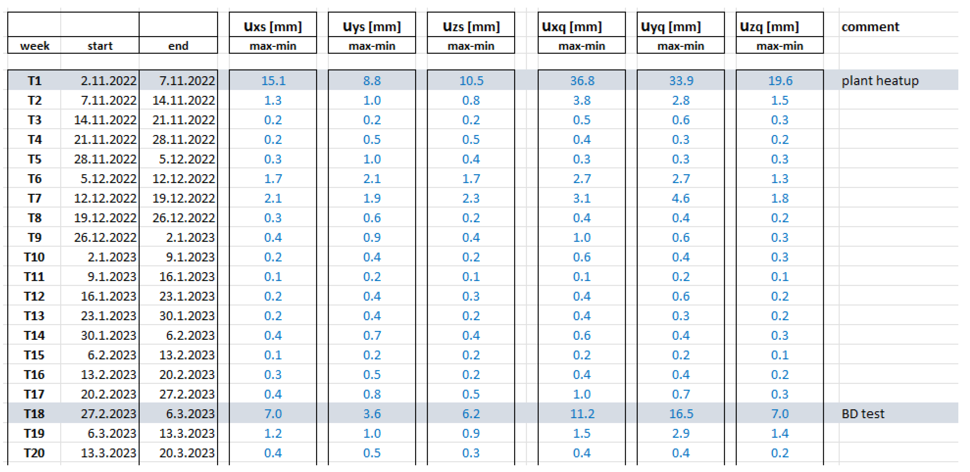
One of basic data analyses is measuring for maximal displacement in each axis. Data is organized in weekly packets, and maximum displacement are stored in a table. Value “max-min” is the difference between maximal and minimal pipe position in a one week time window. Data is calculated for each axis and for both measuring points. In case of any bigger events, that weeks data is being analyzed in detail. Table 1 shows first few months of data from measuring system startup. Excluding the plant startup phase - during which thermal expansion produces expected displacements associated with system heat-up - the largest measured displacements were recorded during week T18 (Figure 13), coinciding with the performance of the Blowdown System test. Outside of this event, the BD system exhibited stable operating behavior, with displacement values remaining constant and within the expected limits.
The Blowdown System test procedure involves the controlled closure of the flow control valves, resulting in gradual variations in both flow rate and temperature within the piping. These slow and continuous changes cause progressive cooling or heating of the pipe. When the valve reaches its fully closed position, a minor pressure transient occurs; however, its magnitude remains well below the threshold that could cause damage to the piping or its supporting structures.
Typical displacement responses recorded during this test are presented in Figure 13 and Figure 14. No abnormal transients were detected, confirming that the test procedure is appropriate and does not introduce any significant additional mechanical stress into the plant equipment.
Figure 14.
typical pipe displacements during BD system test (measuring poins S).
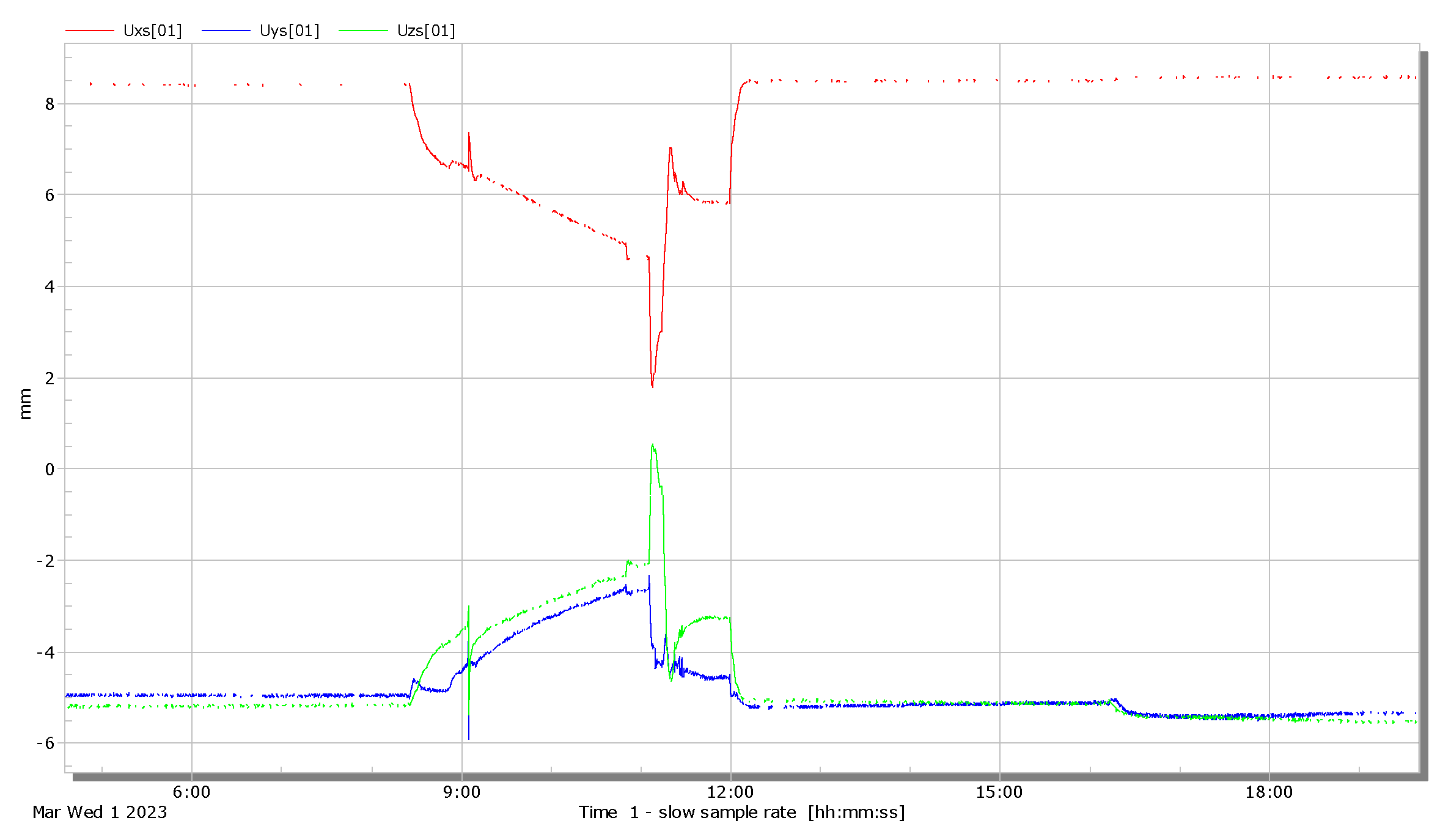
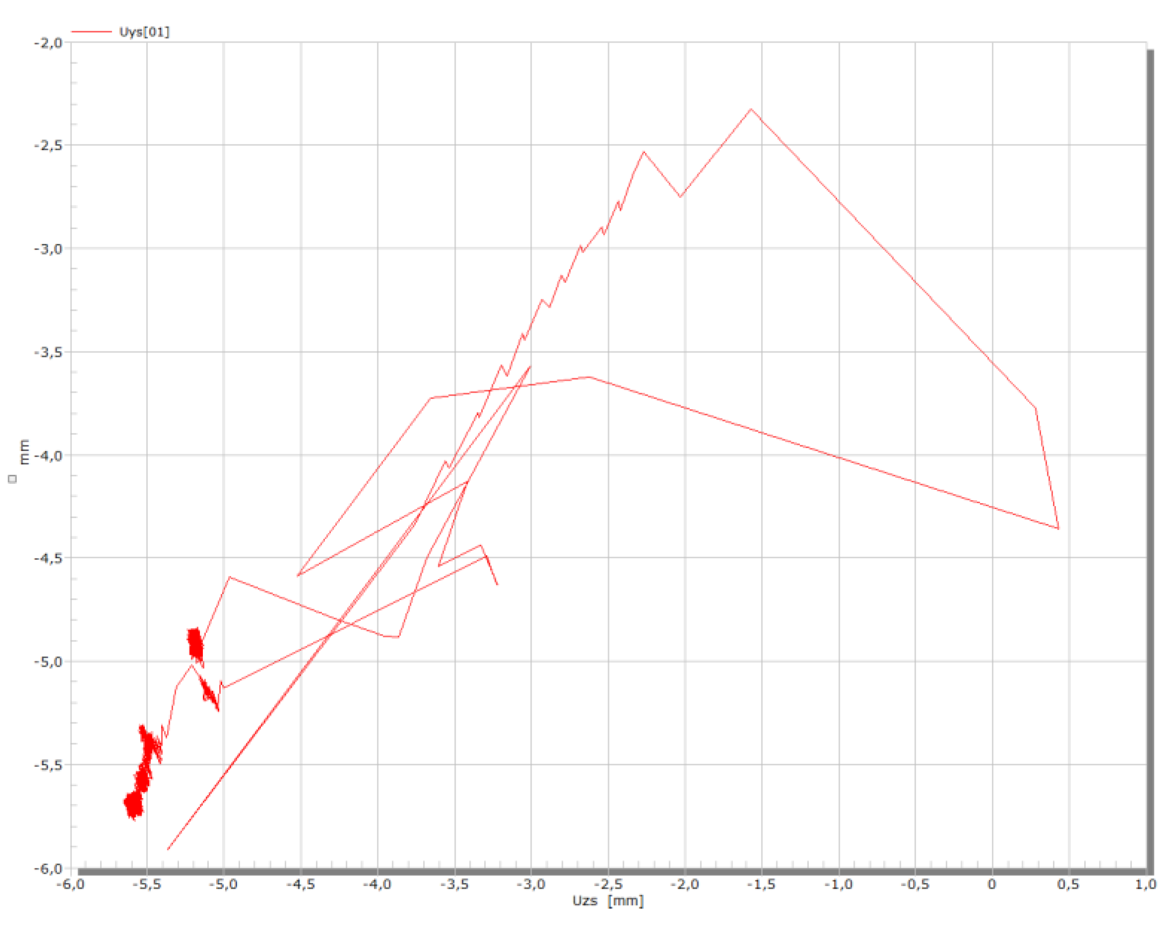
Figure 15.
typical X-Y axis displacement during BD system test (measuring poins S).
4. Conclusions
In high-energy piping systems commonly employed in power-generation facilities including nuclear, thermal, and hydroelectric plants the implementation of an online displacement monitoring system offers substantial operational and diagnostic benefits. Such systems enable
- the verification and optimization of plant operating procedures,
- the identification of root causes of potential damage to pipe support structures,
- the evaluation of post-transient events, and
- the long-term monitoring required for fatigue life assessment of piping components.
To facilitate these functions, a computer-based online displacement monitoring system was developed and implemented at the Krško Nuclear Power Plant. The system was installed on the Steam Generator Blowdown System, a secondary auxiliary subsystem. Two three-dimensional displacement monitoring points were mounted on an 8-inch pipeline conveying a flow rate of 5 to 10 m3/h at a temperature of 180 °C and an operating pressure of 64 bar.
A comprehensive review of available technical literature and industrial applications revealed only one comparable system, which had been implemented on a high-temperature steam pipeline in a gas-fired power plant [1]. No equivalent implementation was identified in other nuclear power facilities. The referenced system employed a robotic-arm-type three-dimensional displacement sensor comprising two rigid arms connected to a fixed base and equipped with two angular sensors and one rotational sensor. Pipe displacement was derived from the known arm lengths and the measured variations in joint angles.
In contrast, the system developed at Krško applies the three non-collinear vector measurement method, as described previously. This approach provides several advantages, including simplified fabrication and installation, reduced mass of the sensor assembly, and a more straightforward calibration procedure.
The system has been operating continuously for a period of three years without requiring major maintenance interventions or exhibiting significant measurement deviations. These results confirm the suitability, reliability, and robustness of both the adopted measurement methodology and the corresponding hardware architecture.
Funding
This project was part of the NPP Krsko maintenance program and therefore funded by NPP Krsko.
Institutional Review Board Statement
Not applicable.
Informed Consent Statement
Not applicable.
Conflicts of Interest
The authors declare no conflicts of interest.
Abbreviations
The following abbreviations are used in this manuscript:
| MDPI | Multidisciplinary Digital Publishing Institute |
| LVDT | Linear Variable Differential Transformer |
| HBM | Hottinger Baldwin Messtechnik |
| NPP | Nuclear Power Plant |
| DAQ | Data Acquisition |
| PIS | Process Information System |
| BD | Steam Generator Blowndown System |
References
- Abdul Ghaffar, M.H.; Lee, D.S.; Husin, S.; Wan Ismail, W.Y. High Temperature Steam Pipe Real-Time Displacement Monitoring System of Gas-Fired Power Plant. In Proceedings of the Conference of the Electric Power Supply Industry 2014, Jeju Island, South Korea, October 2014; Code C.11. [CrossRef]
- Santhosh, K.V.; Roy, B.K. A Smart Displacement Measuring Technique Using Linear Variable Displacement Transducer. Procedia Technology 2012, 4, 854–861. [Google Scholar] [CrossRef]
- Leino, J.; Kokko, V.; Hyvärinen, J. Mapping of Condition Monitoring Systems in Olkiluoto Nuclear Power Plants. Energiforsk Report 2021, No. 785. Available online: https://energiforsk.se/media/29874/mapping-of-condition-monitoring-systems-in-olkiluoto-nuclear-powerplants-energiforskrapport-2021-785.pdf (accessed on 13 November 2025).
- Choi, W.; Han, J. Health-Monitoring Methodology for High-Temperature Steam Pipes of Power Plants Using Real-Time Displacement Data. Appl. Sci. 2021, 11, 2256. [Google Scholar] [CrossRef]
Figure 1.
typical sway struts (blue).
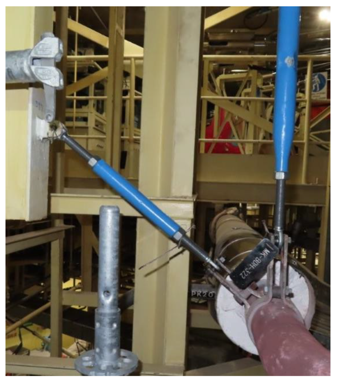
Figure 2.
variable spring.
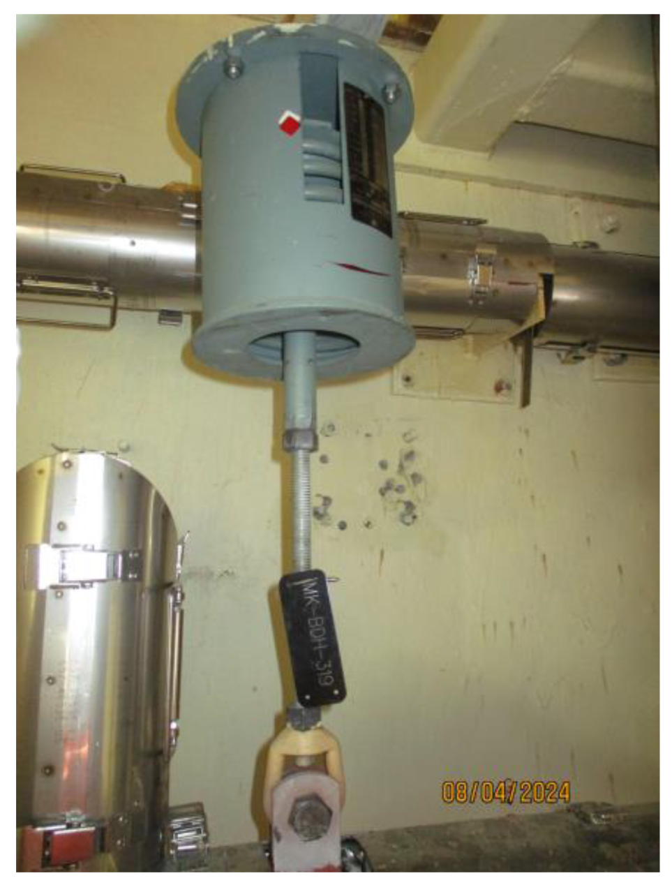
Figure 3.
Spatial representation of the area within which the inductive displacement transducers and the observed point move.
Figure 3.
Spatial representation of the area within which the inductive displacement transducers and the observed point move.
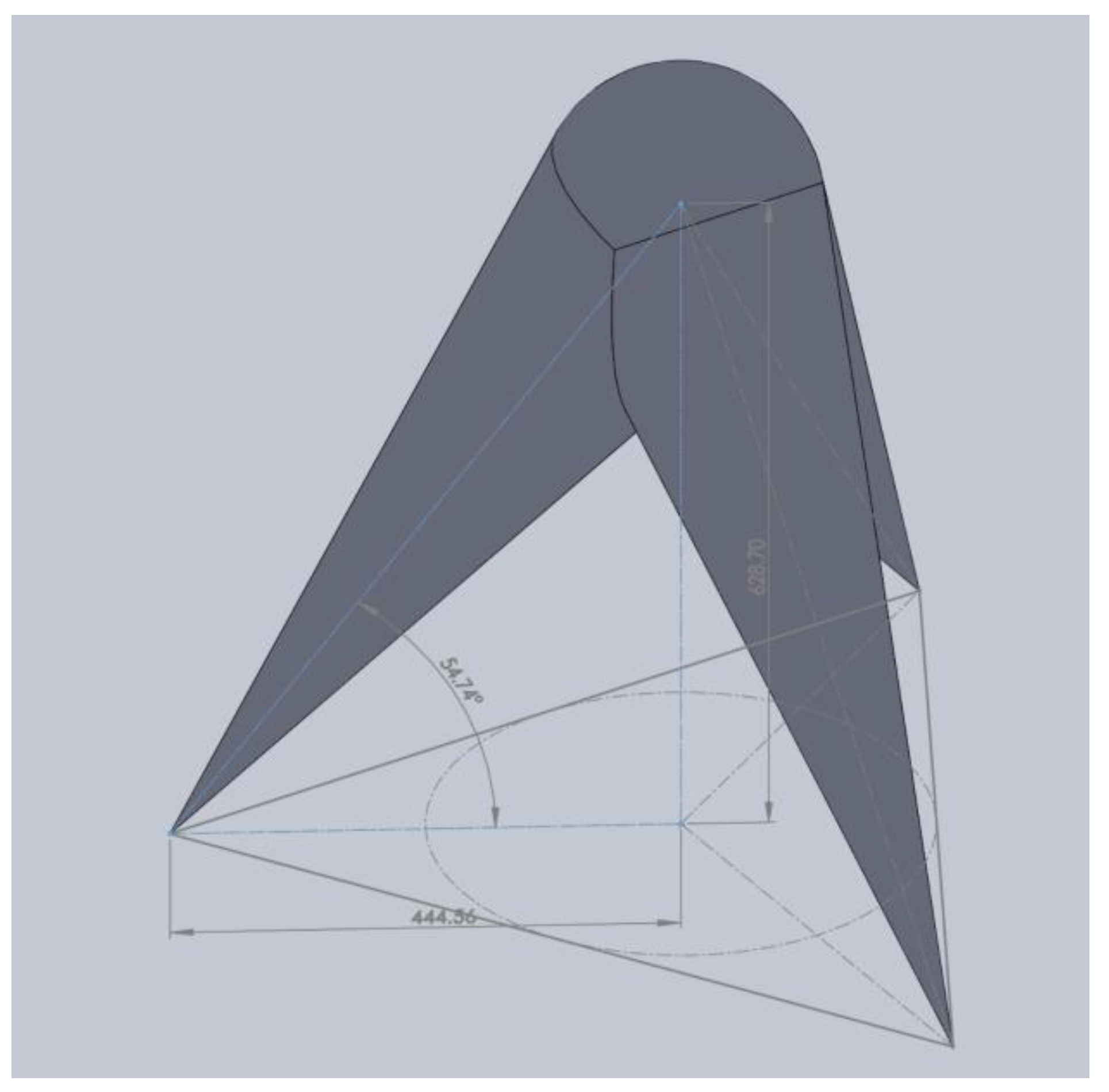
Figure 4.
Geometric representation of the measuring system during the displacement of point to
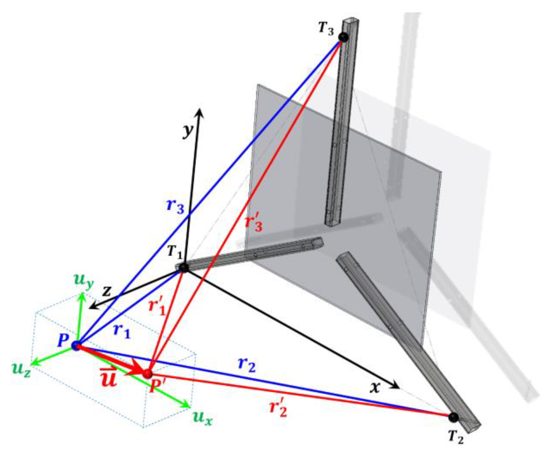
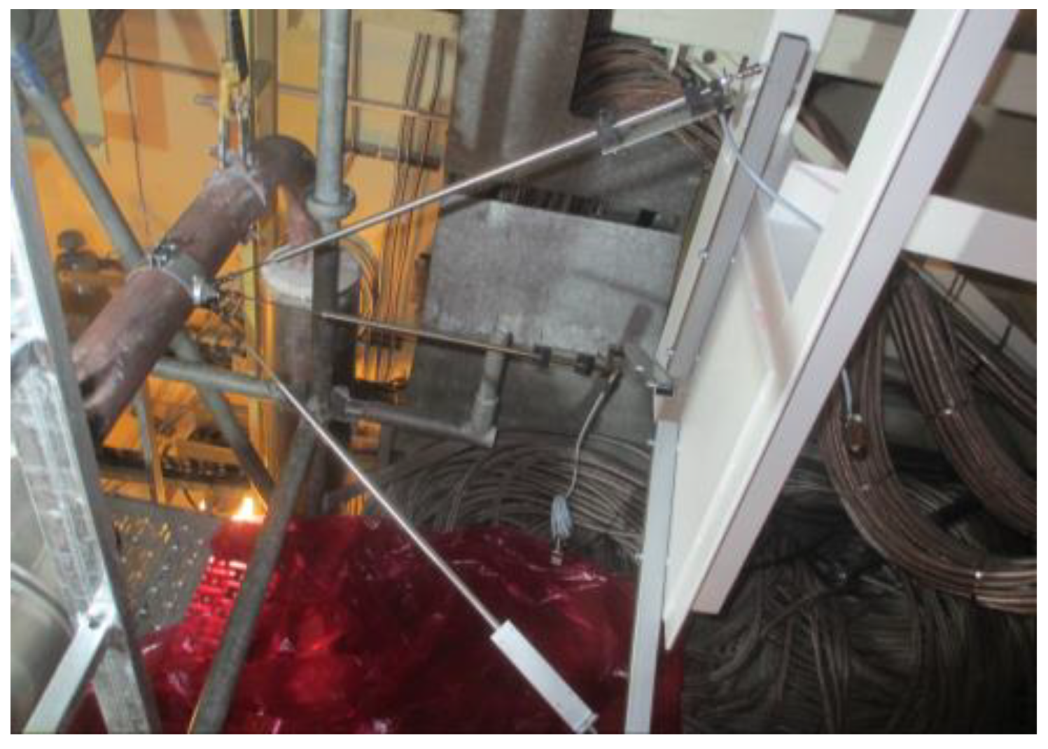
Figure 5.
View of the measurement system at the location S.
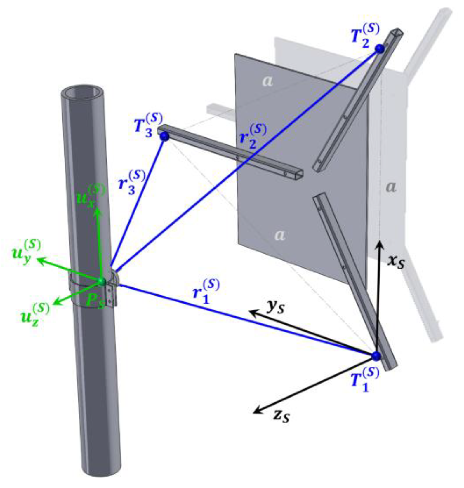
Figure 6.
View of the measurement system at the location Q.
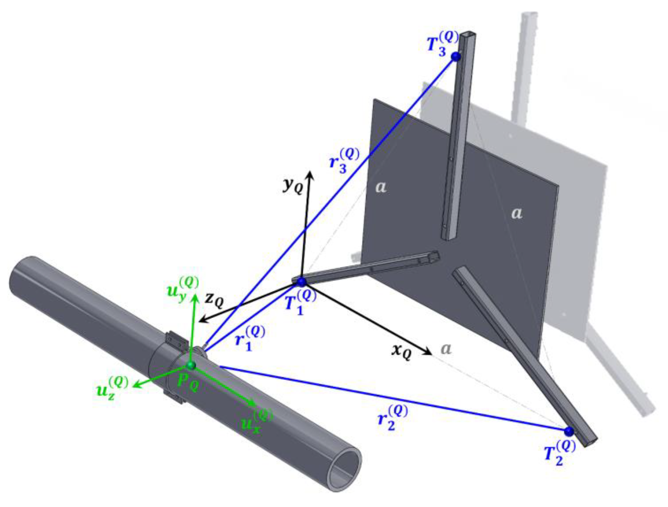
Figure 7.
Location of the points S and Q inside the reactor building.
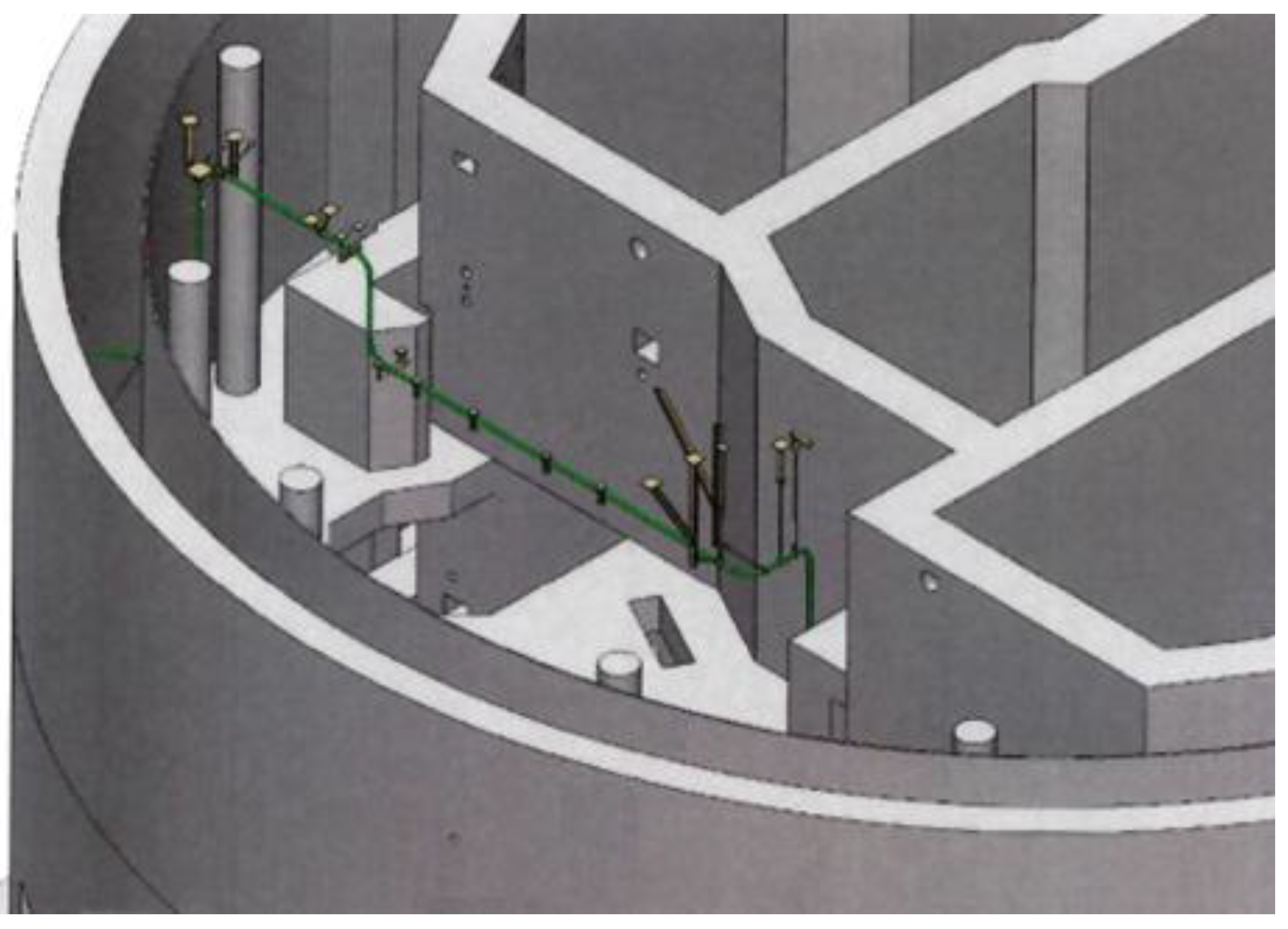
Figure 8.
Mounting of the inductive displacement transducers on the pipe at the observation point S.
Figure 8.
Mounting of the inductive displacement transducers on the pipe at the observation point S.
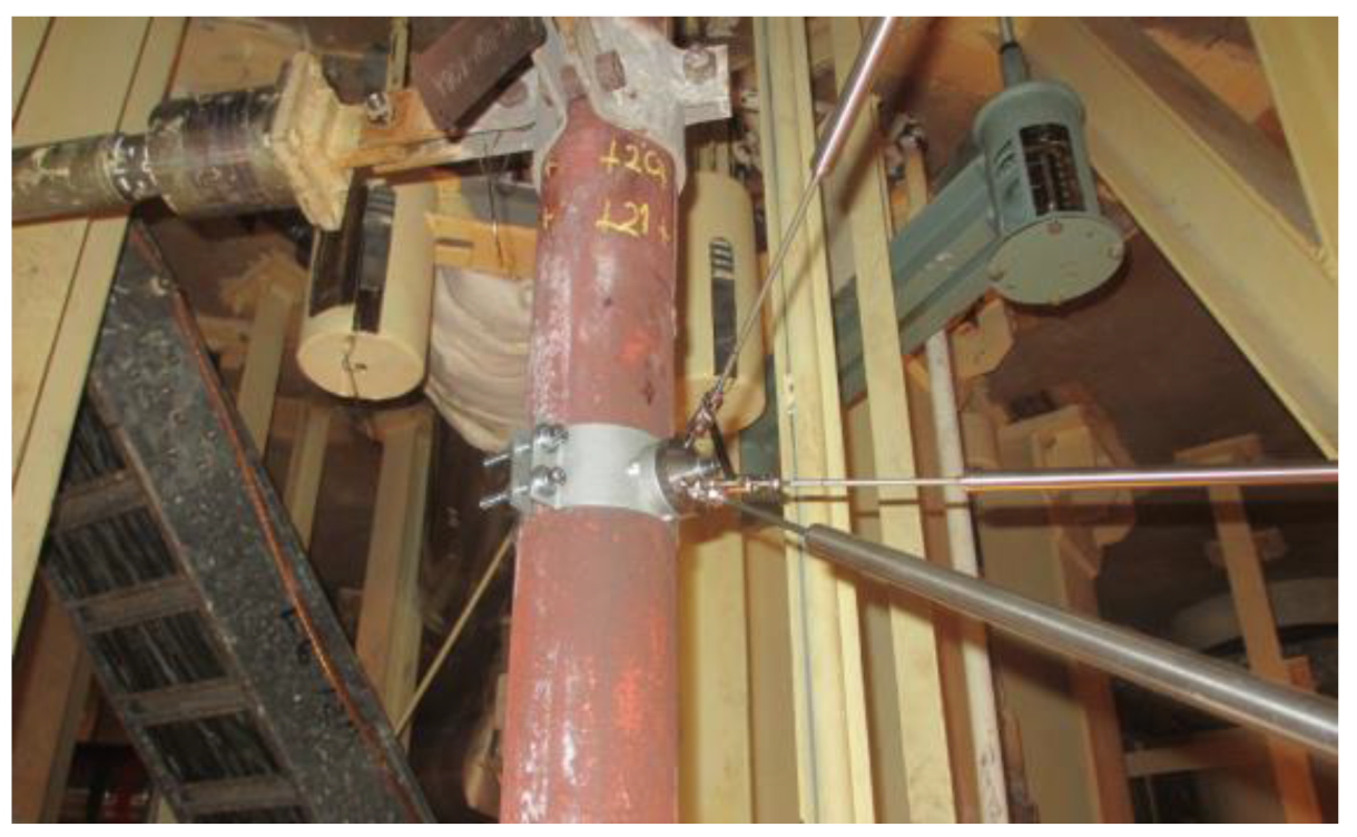
Figure 10.
Measurement system setup.
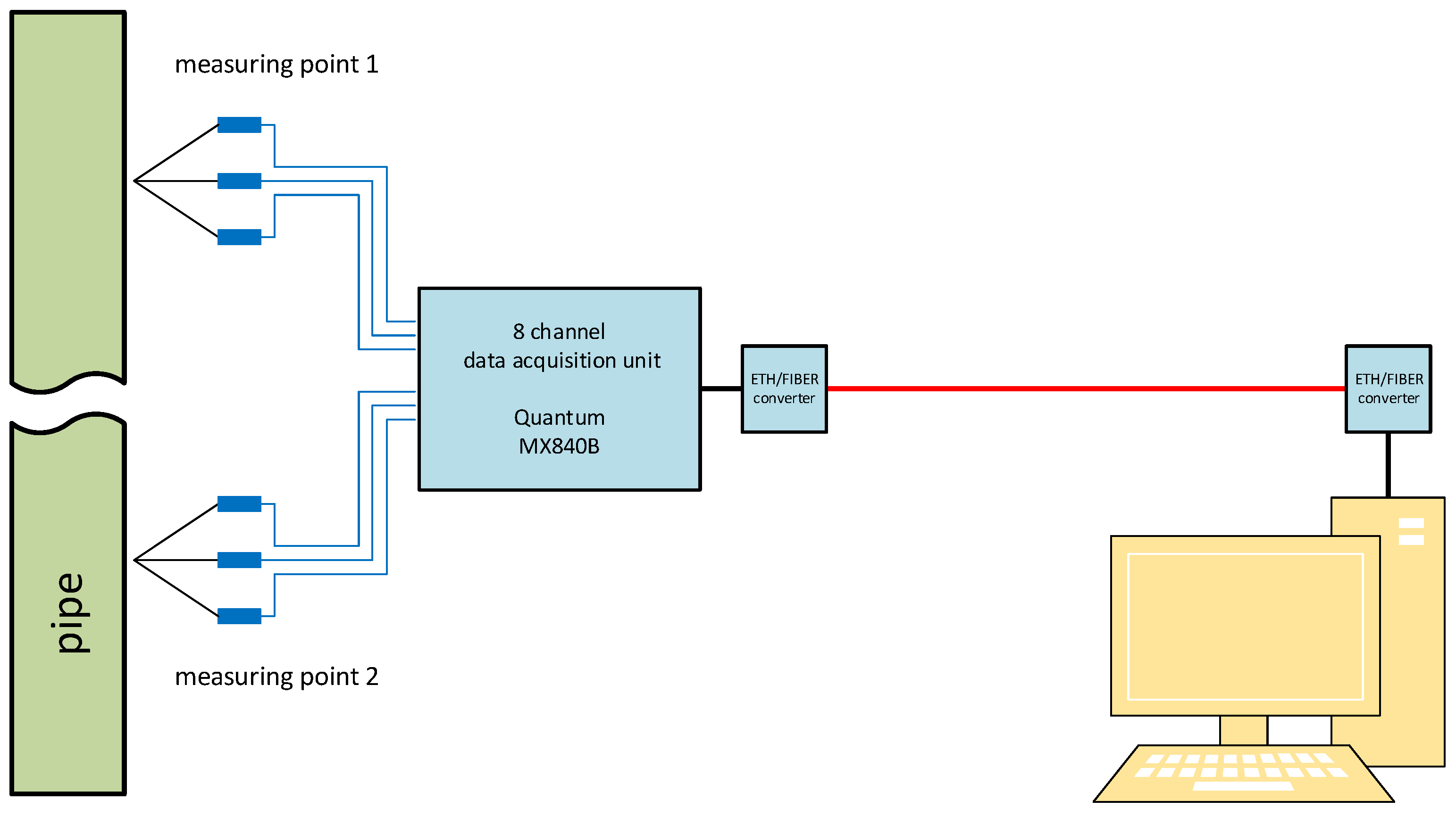
Figure 11.
DAQ unit MX840B.
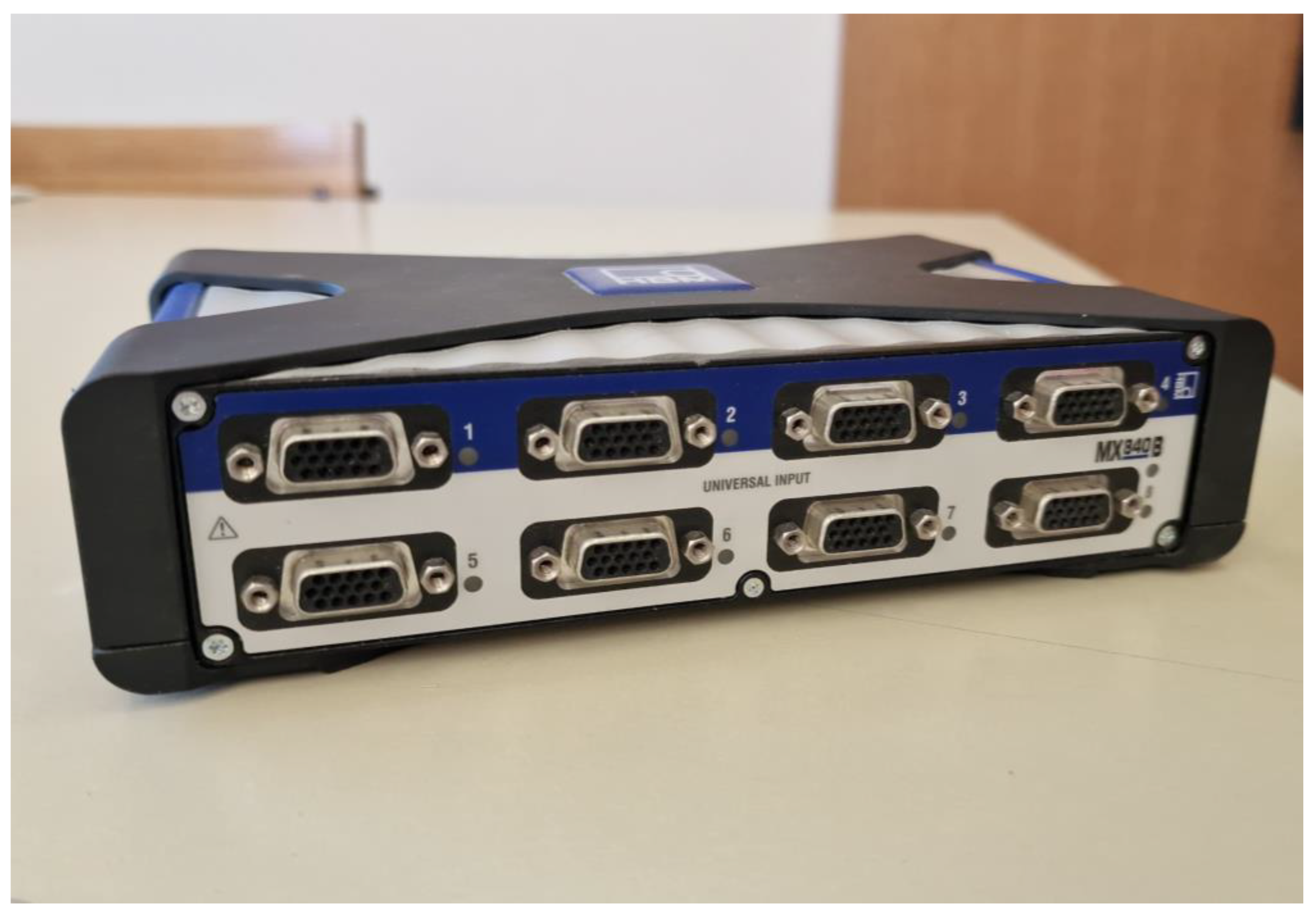
Figure 12.
DAQ cabinet.
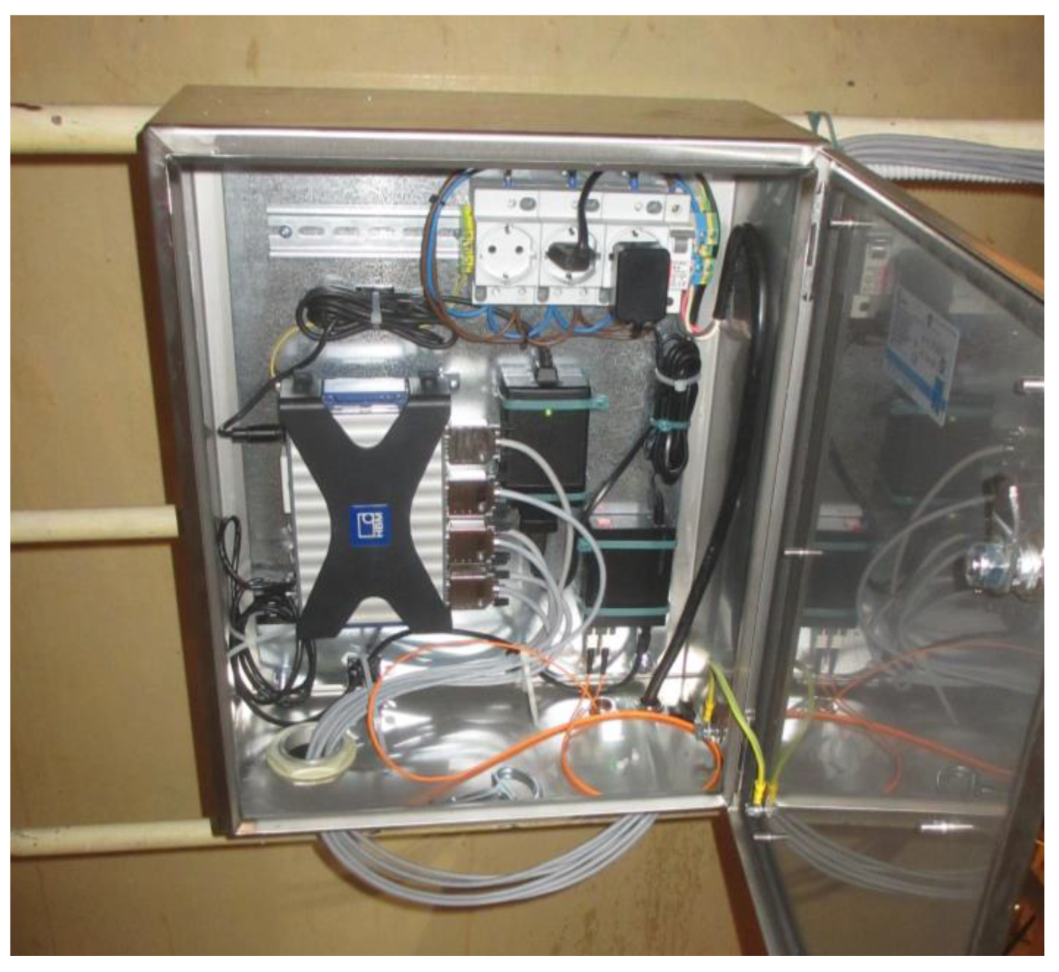
Figure 13.
Printscreen of a maksimum displacements per each week.
Disclaimer/Publisher’s Note: The statements, opinions and data contained in all publications are solely those of the individual author(s) and contributor(s) and not of MDPI and/or the editor(s). MDPI and/or the editor(s) disclaim responsibility for any injury to people or property resulting from any ideas, methods, instructions or products referred to in the content. |
© 2025 by the authors. Licensee MDPI, Basel, Switzerland. This article is an open access article distributed under the terms and conditions of the Creative Commons Attribution (CC BY) license (http://creativecommons.org/licenses/by/4.0/).
Copyright: This open access article is published under a Creative Commons CC BY 4.0 license, which permit the free download, distribution, and reuse, provided that the author and preprint are cited in any reuse.


