
Submitted:
18 October 2024
Posted:
18 October 2024
You are already at the latest version
Abstract
Pipe-type cable systems, including high-pressure fluid-filled (HPFF) and high-pressure gas-filled (HPGF) cables, are widely used for underground high-voltage transmission. These systems consist of insulated conductor cables within steel pipes, filled with pressurized fluids or gases for insulation and cooling. Despite their reliability, faults can occur due to insulation degradation, thermal expansion, and environmental factors. As many circuits exceed their 40-year design life, efficient fault localization becomes crucial. Fault location involves pre-location and pinpointing. Therefore, a novel fully pinpointing approach for pipe-type cable systems is proposed, utilizing accelerometers mounted on the steel pipe to capture fault-induced acoustic signals and employing a time difference of arrival (TDOA) method to accurately pinpoint the location of the fault. Experimental investigations utilized a scaled-down HPFF pipe-type cable system model, featuring a carbon steel pipe, high-frequency accelerometers, and both mechanical and capacitive discharge methods for generating acoustic pulses. Tests evaluated propagation velocity, attenuation, and pinpointing accuracy with the pipe in various embedment conditions. Results demonstrated accurate fault pinpointing within centimeters, even in fully embedded pipes, with acoustic pulse velocities close to theoretical values. These findings highlight the potential of the novel acoustic pinpointing technique presented in this study to improve fault localization in underground systems, enhance grid reliability, and reduce outage. Further research is recommended to validate this technique on full-scale systems.
Keywords:
Acoustic Pinpointing
; Fault Pinpointing
; Fault Location
; HPFF
; Underground Power Transmission
1. Introduction
Underground transmission systems are integral to modern power infrastructure, offering increased reliability and aesthetic benefits over overhead lines [1]. These systems primarily utilize three types of cables: cross-linked polyethylene (XLPE), self-contained fluid-filled (SCFF), and high-pressure fluid-filled (HPFF) or high-pressure gas-filled (HPGF) cables, each with unique characteristics and applications in power transmission [2]. The reliability of these systems hinges on effective fault location techniques and minimized outage durations. In the United States, over 80% of the 4,200 circuit miles of underground high-voltage transmission cables are pipe-type cables, a significant portion of which have approached or exceeded their 40-year design life as of 2007 [3]. The aging infrastructure increases the risk of faults, underscoring the critical need for rapid and accurate fault location methods. A significant majority (69%) of faults occur in cable accessories rather than in the cables themselves, with installation mistakes accounting for 57% of accessory faults. For cable faults, production and installation errors are the primary causes (52%), followed by external damage (17%) and aging (9%) [4]. In HPFF cables, temperature-driven deterioration in oil impregnated paper insulation is a significant issue. This deterioration approximately doubles in rate with every 6°C increase in temperature and is exacerbated by oxygen and moisture ingress [5].
Faults in underground cables can take the form of open circuit faults, short circuit faults, or earth faults, each requiring appropriate identification and resolution [6]. These faults are inevitable and can lead to significant disruptions in power transmission and distribution. Prompt identification and resolution are essential for minimizing revenue losses and reducing customer inconvenience. The fault location process typically involves a two-step approach: prelocation followed by pinpointing. During prelocation, the cable circuit is tested from its terminations to estimate the distance to the fault. Effective prelocation can determine the fault's location within a few percent of the total cable length; however, accuracy may be reduced in very long cables. Some widely used prelocation techniques include time domain reflectometry (TDR), burn down, and arc reflection [7,8,9]. The choice of prelocation technique often depends on the fault type and cable characteristics, as no single method is universally optimal.
Pinpointing the exact fault location of underground cables can be accomplished through various techniques. A voltage gradient method involves applying a pulsed direct current (DC) voltage to the faulted cable, creating a voltage gradient in the surrounding soil. This voltage gradient can be measured with earth probes to locate the fault, particularly effective for direct-buried cables but less accurate in highly resistive soils or ducts [10,11]. A magnetic gradient method detects the magnetic field from an alternating current (AC) voltage injected into the cable, useful for submarine cables but less effective in complex urban environments [12]. An acoustic method is the conventional approach for fault pinpointing and involves using "capacitive discharge" techniques [13]. This acoustic method involves discharging an electrical impulse onto the cable with a high-voltage test set, causing it to break down at the fault’s location. The sound of the breakdown pulse is then picked up acoustically. This is commonly referred to as ‘thumping’. The pinpointing method is accomplished by operators using specialized surface microphones (geophones) and walking along the cable route. While this pinpointing method is very effective, it is burdened by an extremely slow response time due to setup, methodical search along the cable route, and interference or noise effects in the subsurface environment. Additionally, repeated thumping may cause further damage to the cable [14]. Locating faults in ducted cable systems can also be challenging. Poor acoustic contact may prevent the fault from generating a detectable signal at the surface, with the acoustic signal traveling along the duct and the strongest signal often detected at nearby manholes rather than directly at the fault site [15].
In recent years, newer fault location methods for underground cables, such as distributed temperature sensing and distributed vibration sensing, have shown promise in fault location [12]. These fault location methods utilize fiber-optic cables embedded alongside power cables to detect variations in temperature and vibration caused by faults. While these fault location methods offer real-time monitoring and high precision, they require pre-installed fiber optics, which are not always available in legacy systems. Another growing trend is the integration of IoT-based systems, which combine technologies such as LTE, GPS, and GSM, along with electric field energy harvesters as power sources, to enable real-time fault detection and location [16,17,18,19,20,21,22,23]. These IoT-based fault location methods enable remote monitoring but are typically part of online systems that must be installed before a fault occurs, making them less practical for older circuits lacking such infrastructure. The limitations of current fault pinpointing methods, particularly for aging pipe-type cable systems in complex environments, highlight a critical gap in the field. While recent advancements focus on real-time, pre-installed systems, there is a pressing need for innovative offline solutions applicable to existing infrastructure. Current techniques, though offering certain advantages, fail to fully address the unique challenges posed by urban infrastructure and ducted systems. An ideal solution would leverage advanced sensors and technology for rapid, accurate, and non-damaging fault location, while building upon the strengths of acoustic detection methods.
To address these challenges, this study proposes a novel enhancement to conventional acoustic thumping for pipe-type cable systems. Rather than relying on the traditional method of walking the entire cable route with a geophone, the proposed pinpointing approach for pipe-type cable systems involves accessing nearby manholes and attaching acoustic sensors directly to the steel pipe after fault prelocation estimation. This innovative method, inspired by the concept of acoustic leak location as detailed in previous research [24,25,26,27,28], aims to offer a more efficient and accurate means of fault pinpointing. Hydrophones, geophones, and accelerometers were evaluated as candidate sensors for steel-borne acoustic pinpointing [29,30,31]. Among these, an accelerometer-based instrumentation package was identified as offering the best pinpointing accuracy, particularly for detecting acoustic pulses in steel pipes with low damping and a high signal-to-noise ratio [32]. Various signal processing techniques, such as Fast Fourier Transforms (FFT), Wavelet Transforms (WT), cross-correlation, and empirical mode decomposition (EMD), have been successfully applied to acoustic wave propagation in pipes [33,34,35]. While these methods can enhance data interpretation, this study focuses on validating direct accelerometer measurements for fault location. Future work may explore the integration of advanced signal processing techniques to further refine pinpointing accuracy. By utilizing accelerometers in this enhanced setup, the proposed method aims to detect high-frequency steel-borne acoustic pulses with greater sensitivity and provide immediate and significantly improved fault pinpointing accuracy with just a single thump. Additionally, this approach minimizes the potential damage caused by repeated thumping inherent in conventional methods, which often involve manual searching with a geophone.
The main objective of this study is to validate the proposed concept of steel-borne acoustic fault pinpointing by replicating the thumping mechanism in the lab and carrying out an experimental study on a scaled-down HPFF test rig. The study will focus on determining the acoustic pulse propagation characteristics, evaluating pinpointing accuracy, and assessing how surrounding backfill material affects signal attenuation. The results will demonstrate the feasibility of this enhanced method in improving fault pinpointing for HPFF pipe-type cables. The successful implementation of this advanced acoustic pinpointing method could significantly improve the reliability and resilience of underground power distribution networks, potentially reducing downtime, minimizing repair costs, and enhancing overall grid stability across urban and suburban areas.
The rest of this paper is organized as follows: in Section 2, the test setup, instrumentation and testing methodologies are outlined. In Section 3, the results of all test cases are presented, while Section 4 discusses the results. Finally, the conclusions are summarized in Section 5. The rest of this paper is organized as follows: Section 2 details the experimental setup, including the scaled-down HPFF test pipe, instrumentation, and testing methodologies for acoustic pulse generation and detection. Section 3 presents the results, covering acoustic pulse velocity measurements, fault localization accuracy, and attenuation studies under various pipe embedment conditions. Section 4 discusses the implications of the results, primarily discussing the potential of this technology for fault pinpointing and describing the benefits over traditional method. comparing the findings to conventional acoustic fault pinpointing methods. Section 5 summarizes the conclusions drawn from this study. Finally, Section 6 suggests directions for future work.
2. Experimental Setup: Materials and Methods
Acoustic pinpointing feasibility testing was conducted on an experimental test pipe consisting of a 19-m (49.25 mm ID) Schedule-80 carbon steel pipe, the same material used in HPFF pipes. The pipe was coated externally with Pritec (HDPE over butyl mastic), the same as that used in HPFF pipes. The pipe's dimensions and material properties are summarized in Table 1. The measurement system included four B&K accelerometers, two B&K two-channel signal conditioners, and one Delphin Expert Transient Data Logger, with specifications provided in Table 2, Table 3 and Table 4. Figure 1 depicts the test pipe and the components of the measurement system.
The accelerometers were individually calibrated by the manufacturer using state-of-the-art random FFT technology, providing an 800-point high-resolution calibration (magnitude and phase). Prior to testing, the accuracy of the sensors' calibration and time synchronization was verified by attaching them at the pipe's end and impacting the test pipe at the opposite end, as illustrated in Figure 2 by Locations 1 and 4. The resulting waveforms recorded by sensors show a high degree of calibration and time synchronization across the entire sensor array, as shown in Figure 3. The sensors were strategically attached to the steel pipe using beeswax, positioned at both ends and at one-third intervals along its length. These positions, designated as Locations 1, 2, 3, and 4, are shown in Figure 2. This configuration enabled comprehensive data collection along the entire pipe length.
Two methods were employed for acoustic pulse generation in the test pipe for this study. The first method utilized a weight drop apparatus where a 0.91-kg (2-lb) weight was released from a fixed height of 63.5 mm (2.5 in) onto the pipe’s surface. This method ensured consistent and repeatable acoustic pulse generation, enabling standardized measurements across multiple tests and runs.
The second method employed a fault simulator device designed to more closely mimic the real-world fault thumping mechanism. This custom-built device comprised of a non-resistor spark plug, retrofitted into the dielectric fluid filled as will be detailed in Section 2.2. The terminals of the fault simulator device connect to a surge wave generator or a full-scale thumper, enabling powerful capacitive discharges at the spark gap. The specifications of the full-scale thumper are detailed in Table 4.

Table 4.
Specifications of the Megger 32 kV Thumper.
| Item | Value | |
|---|---|---|
| Product model | Megger SPG 32 | |
| Voltage Energy Surge Rate Burning |
0 – 32 kV 1750 Joules 3 – 10 s; single pulse 0 – 32 kV; 160 mA |
2.1. Test Series 1
2.1.1. Test 1.1: Determining and Verifying Acoustic Pulse Velocity in Steel Pipe
To accurately pinpoint the source of an acoustic pulse along the length of the pipe, it is essential to determine the acoustic pulse velocity in the steel pipe experimentally and verify against the theoretical value. In Test 1.1, an acoustic pulse was generated at Location 1 using the weight drop apparatus. The time of flight across the 19-meter test pipe was measured by cross-correlating the pulse's arrival time at Location 4 with its initiation time at Location 1. The experimental velocity of the acoustic pulse was then calculated using the distance and measured time, while the theoretical velocity of the acoustic pulse can be determined by
where E is the Young's modulus of the material and ρ is the density of the material.
2.1.2. Test 1.2: Localization Accuracy and Pinpointing of Acoustic Pulse Source
With the propagation velocity established, Test 1.2 aimed to investigate the fault pinpointing concept and evaluate localization accuracy by generating an acoustic pulse at one-third of the pipe length (Location 2). The acoustic pulse source is pinpointed by using the Time Difference of Arrival (TDOA) method, which can be represented as
where d is the total length of pipe (d=19m) and ∆t is the TDOA.
2.2. Fault Simulator Device Evaluation for Acoustic Pulse Generation
For the proposed technology to be viable for HPFF fault pinpointing, thumping of the cable system must vaporize the dielectric fluid surrounding the fault. The sudden vaporization of the dielectric fluid creates a shock wave, which is believed to induce an acoustic pulse that propagates inside the pipe’s wall in both directions. To investigate this concept, the test pipe was equipped with necessary hydraulic components and filled with dielectric fluid type DF 100, a fluid very commonly used in HPFF cable systems. The fault simulator device was then installed in the test pipe and connected to the Surge Wave Generator, as shown in Figure 5. Test 2 was conducted to validate the concept that creating a fault generates an acoustic pulse in the steel wall. This test involved producing a capacitive discharge (spark) in the dielectric fluid at Location 1. The goal was to generate a steel-borne acoustic pulse that could be detected by Sensor 4 at the remote end of the pipe. This test laid the groundwork for more comprehensive future testing.
2.3. Test Series 3: Acoustic Pulse Attenuation Study
In actual HPFF pipe-type cable installations, the steel pipe is mechanically coupled to the surrounding soil, resulting in increased signal attenuation due to the leakage of acoustic energy into the soil. To explore this complex interaction, Test 3 was conducted as a series of subtests (Tests 3.1–3.3), designed to investigate the effects of varying embedding conditions on the propagation and attenuation of steel-borne acoustic pulses. The tests included conditions where the pipe was: fully supported in air (Test 3.1), laid on tamped rock dust (Test 3.2), and finally fully embedded in tamped rock dust (Test 3.3). Rock dust, selected for its excellent thermal properties and common use in engineered backfill, served as the backfill material. Its grain composition, which ranges from coarse to fine, allows for high compaction and thermal conductivity, providing a controlled medium to analyze acoustic energy absorption and signal attenuation.
In each subtest (Tests 3.1–3.3), a consistent acoustic pulse was generated using the weight drop apparatus, with a 0.91 kg (2 lb.) weight dropped from a constant height of 63.5 mm (2.5 in) at the pipe end (Location 1). The four accelerometers were evenly spaced along the 19-meter pipe at one-third intervals (6.33 meters apart). To ensure reliability and repeatability, five identical runs were recorded for each subtest. A 3 kHz low-pass filter (LPF) was applied to the data to remove high-frequency noise and enhance the clarity of the acoustic pulse signals. This filter was used because it was observed in previous tests that the acoustic pulse frequency components resided within this range. The filtered data was then collected and analyzed to assess the impact of different embedding conditions on signal attenuation.
The attenuation constant between sensors was calculated using Equation (3), where A0 is the reference amplitude and A1 is the amplitude of the acoustic pulse after traveling a distance L.
2.3.1. Test 3.1: Pipe Supported in Air – Attenuation of Pipe in Air
In Test 3.1, the test pipe was supported in air using four V-head pipe stands, identical to the setup in Test Series 1 and 2. This test aimed to assess the attenuation of the acoustic pulse due solely to the pipe's properties, serving as a baseline reference for evaluating additional damping effects observed in Tests 3.2 and 3.3. Figure 6 depicts the setup for Test 3.1, showing the pipe supported in air along with the location of the weight drop apparatus.
2.3.2. Test 3.2: Pipe Laid on Tamped Backfill – Attenuation due to Contact with Backfill
For Test 3.2, a containment box measuring 17 m in length, 46 cm in width, and 61 cm in height was constructed from plywood and lined with a vinyl sheet to prevent moisture ingress. Aluminum foil was placed at the bottom of the box to provide grounding for future thumping tests. The pipe was placed on top of the 15 cm thick layer of tamped rock dust, which was added and tamped in 5–8 cm lifts. The overall test layout with the dimensions of the tamped rock dust is shown in Figure 7. The tamping and layering process are depicted in Figure 8a,b, and the final set up is shown in Figure 8c. As in Test 3.1, controlled weight drops were performed using the weight drop apparatus from the same height, maintaining all parameters consistent except for the pipe now being supported on the tamped rock dust.
2.3.3. Test 3.3: Attenuation in Fully Embedded Pipe
In Test 3.3, additional layers of rock dust were added and tamped until the pipe was fully embedded in the center of the containment box, as shown in Figure 9 and Figure 10a. Access point to the intermediate sensors via a 'manhole' is shown in Figure 10b. The fully surrounding backfill material (rock dust) provided an absorbing medium for acoustic energy, similar to real pipe-type cable systems. Controlled weight drops were performed using the weight drop apparatus, with all parameters consistent with Tests 3.1 and 3.2, except that the pipe was now fully embedded in backfill.
2.4. Test 4 - Fault Simulator Thumping Test on Fully Embedded Test Pipe
Test 4 evaluated the acoustic pinpointing method in the fully embedded, dielectric fluid-filled test pipe configuration of Test 3.3. The fault simulator was positioned at one-third of the pipe's length (Location 2). A full-scale commercial thumper applied a 16 kV voltage charge to the spark plug, simulating a cable fault at an intermediate location. Figure 11 depicts the complete test setup, which represents a comprehensive, scaled-down model of a real HPFF system. The objective of this experiment was to assess the effectiveness of acoustic pinpointing under conditions that closely mimic those of an actual HPFF system within a controlled laboratory environment.
2.5. Summary of Experimental Tests
Table 6 provides a summary of all the tests conducted in this study, highlighting the objectives, acoustic pulse generation methods, and corresponding embedment conditions for each test case.
3. Experimental Results
3.1. Test Series 1
3.1.1. Test 1.1: Determining and Verifying Acoustic Pulse Velocity in the Test Pipe
In Test 1.1, an acoustic pulse was induced at the pipe’s end (Location 1). The sensors at Locations 1 and 4 captured the complete waveforms of this acoustic event, as shown in Figure 12. Cursor 1 indicates the timestamp of when the acoustic pulse was induced at Location 1 (Sensor 1, blue trace), and Cursor 2 indicates the timestamp of the time of arrival of the acoustic pulse at Location 4 (Sensor 4, red trace). The acoustic pulse's time of flight across the 19-meter pipe was approximately 3.75-3.8 ms, as shown in the cross-correlated close-up snapshot in Figure 13. This yields an experimental propagation velocity of 5,000-5,066.67 m/s, closely matching the theoretical velocity of 5,047.7 m/s (calculated using E = 200 GPa and ρ = 7,850 kg/m3 in Equation 1). Multiple test runs were conducted, and all yielded the same results with a max difference of about 0.1 ms between runs. The slight discrepancy between test runs can be attributed to high-frequency wave timestamping limitations. While advanced signal processing might reduce this error, the current accuracy is sufficient for this study's proof of concept purpose.
3.1.2. Test 1.2: Localization Accuracy when Pinpointing the Source of an Acoustic Pulse
In Test 1.2, to evaluate the viability and accuracy of the acoustic pinpointing concept, an acoustic pulse was induced at one-third of the pipe’s length (Location 2). Figure 14 illustrates the TDOA of the acoustic pulse at the pipe ends, which was measured as 1.249 ms. In Figure 14, Cursor 1 indicates the arrival time at Location 1 (Sensor 1, blue trace), while Cursor 2 indicates the arrival time at Location 4 (Sensor 4, red trace).
Using Equation 2, with ∆t = 1.249 ms, v = 5,047.7 m/s, and d = 19 m, the acoustic pulse’s origin was calculated to be 6.34 m from Location 1. This closely matches the actual source location of 6.333 m (one-third of the pipe length). The centimeter-level accuracy achieved in this test suggests that if cable thumping generates a sufficiently strong acoustic pulse that propagates along the steel pipe wall and can be detected by remotely positioned sensors, precise fault pinpointing may be feasible.
3.2. Test 2: Acoustic Pulse Induced by Simulated Fault Thumping in Test Pipe
Test 2 involved creating an arc (spark) in the dielectric fluid inside the pipe at Location 1, simulating the arcing mechanism that occurs at the fault location when a cable is thumped. The waveforms recorded by the sensors installed at the pipe ends are shown in Figure 15. The results indicate that a capacitive discharge in the dielectric fluid not only creates a hydraulic pressure transient but also induces an acoustic pulse that propagates inside the steel pipe wall. This test further validates the acoustic fault pinpointing concept, confirming that thumping a real HPFF pipe-type cable system will very likely induce an acoustic pulse at the fault’s location. The acoustic pulse velocity of 3.76 ms was consistent with that derived in Test 1.1, as expected, since acoustic velocity depends on the propagation medium regardless of the generation method.
3.3. Test Series 3
3.3.1. Test 3.1
In Test 3.1, the pipe was supported in air similar to the previous tests. An acoustic pulse was induced at the pipe end (Location 1) via the weight drop apparatus (0.91 kg dropped from a 63.5 mm height). Five identical test runs were conducted from the same height with a 3 kHz LPF was applied to the experimental data. Overview of the five test runs is shown in Figure 16 and the waveforms of Test 1 – Run 1 as acquired from the 4 sensors are shown in Figure 17. The waveform peak amplitudes from Sensors 1, 2, 3, and 4, as labeled in Figure 17, were recorded for all five runs and were tabulated in Table 6.
Table 6.
Peak amplitudes at each of the four locations (Test 3.1).
| Title 1 Run# | Sensor 1 Peak (mV) | Sensor 2 Peak (mV) | Sensor 3 Peak (mV) | Sensor 4 Peak (mV) |
|---|---|---|---|---|
| 1 2 3 4 5 |
1333 | 618.9 | 438.3 | 308.5 |
| 1481.5 | 714.5 | 505.3 | 346.8 | |
| 1493.3 1582.5 1511 |
720 778 729.1 |
511.9 551.9 521.1 |
353.6 379.8 351.4 |
|
| Average | 1480.3 | 712.1 | 505.7 | 348.0 |
| % Decrease | 51.9% | 29% | 31.1% | |
| Atten. Coefficient | 0.116 Np/m | 0.054 Np/m | 0.059Np/m |
Attenuation of the acoustic pulse is evident as shown in Figure 17 and summarized in Table 6. Table 6 also shows that the peak amplitudes between runs were consistent, confirming the reliability of the excitation method and the repeatability of the test setup. The peak amplitude decreased by approximately 52% between Sensor 1 and Sensor 2, 29% between Sensor 2 and Sensor 3, and 31% between Sensor 3 and Sensor 4. This pattern of attenuation was consistent across all five test runs.
To determine the overall attenuation over the entire 19-meter pipe, the average peak amplitude from each of the four sensors was plotted in Figure 18. This figure illustrates how the signal’s peak value attenuates as it propagates along the length of the pipe. The overall attenuation coefficient, determined to be 0.074 Np/m from the power of the exponential function in the trendline equation, will serve as a reference for assessing the added attenuation due to pipe embedment in subsequent tests.
3.3.2. Test 3.2
Test 3.2 replicated the procedure of Test 3.1, with the sole modification being the test pipe's placement on tamped backfill rather than being supported in air. The waveforms acquired from the 4 accelerometers for a representative run (Run 1) are shown in Figure 19. The acoustic pulse peak amplitude at each location for the five test runs are detailed in Table 7.
The attenuation of the acoustic pulse is evident as shown in Figure 19 and summarized in Table 7. The percentage decrease in peak amplitude from Sensor 1 to Sensor 2 was approximately 56.7%, 35% between Sensors 2 and 3, and 38.2% between Sensors 3 and 4. Figure 18 depicts the overall attenuation of the acoustic pulse as it propagates along the 19 m pipe. The overall attenuation coefficient for Test 3.2 was measured at 0.09 Np/m. A slight increase in the attenuation coefficient of approximately 0.016 Np/m was observed between Tests 3.1 and 3.2. This increase is attributed to the pipe's contact with tamped soil, which resulted in minor acoustic energy leakage.
3.3.3. Test 3.3
Test 3.3 replicated the testing procedure of Test 3.1 and 3.2, except the pipe was now fully embedded in backfill. The waveforms acquired from the 4 accelerometers for a representative run (Run 1) are shown in Figure 21. The acoustic pulse peak amplitude at each location for the five test runs are detailed in Table 8.
Analysis of the Test 3.3 data in Table 8 indicates that the percentage decrease in peak amplitude from Sensor 1 to Sensor 2 was approximately 86%, increasing to 94.3% between Sensors 2 and 3, and measuring at 66.9% between Sensors 3 and 4. This attenuation pattern remained consistent across all five test runs. The overall average attenuation across the 19 m embedded pipe for Test 3.3 was calculated to be 0.327 Np/m, as shown in Figure 22. This reflects an increase by a factor of 3 compared to the attenuation levels recorded in Tests 3.1 and 3.2, which is attributed to acoustic energy leakage into the surrounding backfill medium. The data demonstrate that the acoustic pulse amplitude decreased from an initial 1670 mV to 4.7 mV after propagating the entire 19 m pipe length. However, despite this substantial reduction, the pulse remained clearly detectable after traveling 19 m, highlighting the potential viability of this method for long-distance acoustic pulse detection in fully embedded pipe conditions.
3.4. Test 4: Fully Embedded Fault Simulator Pinpointing Test
Following the assessment of backfill material's impact on acoustic pulse attenuation, we confirmed that a low-amplitude pulse generated by the weight drop apparatus was detectable after propagating 19 meters in the fully embedded pipe. Subsequently, a test was conducted using a fault simulator and a full-scale commercial thumper, which applied a 16 kV voltage charge to simulate a fault thumping event at one-third of the pipe’s length (Location 2). Figure 13 shows the acoustic pulse waveform as obtained from the time-synchronized sensors at the pipe's ends (Sensors 1, blue and Sensor 4, red).
The results of the fault simulator test on the fully embedded pipe indicate that even when the test pipe is fully embedded in backfill, the instrumentation package can readily detect and timestamp the acoustic pulse waveform generated at the fault’s location using sensors positioned remotely (Figure 22). A time of arrival difference of 1.266 ms was deduced between Sensors 1 and 4. Using Equation 2, with ∆t = 1.266 ms, v = 5,047.7 m/s, and d = 19 m, the fault induced acoustic pulse origin was calculated to be 6.305 m from the pipe's end. This result closely aligns with the actual fault location at 6.333 m (one-third of the pipe length).
These findings indicate that pinpointing the simulated fault in the scaled-down HPFF test setup was accurate to within 2.5 cm, representing an accuracy of 0.13% of the pipe’s 19 m length. This demonstrates the potential of acoustic fault pinpointing for HPFF pipe-type cable systems, suggesting that high precision may be achieved within a typical test setup. However, validation on a full-scale system is necessary.
4. Discussion
The studies presented in this paper offer significant insights into the feasibility and accuracy of a novel acoustic fault pinpointing technique within a scaled-down model of an HPFF pipe-type cable system. Employing a 19-meter test pipe, our experiments demonstrated high accuracy in both measuring acoustic pulse velocity and localizing faults under controlled conditions. The measured velocity, ranging from 5,000 to 5,066.67 m/s, closely aligned with the theoretical value of 5,047.7 m/s, validating the measurement methodology used in this study. Additionally, fault simulation tests conducted on the fully embedded configuration confirmed the potential applicability of this technique. Using a commercial thumper, we successfully detected and accurately localized a simulated fault to within 2.5 cm over the 19 m pipe, demonstrating potential for fault pinpointing in full-scale systems. The effect of pipe embedment on acoustic pulse attenuation was clearly demonstrated in Test Series 3. Attenuation progressively increased as we moved from the pipe suspended in air to partially and fully embedded conditions. Specifically, an attenuation coefficient of 0.074 Np/m was measured between Sensors 1 and 4 in the air-supported setup. This value increased to 38.2% when the pipe was laid on tamped backfill, and further to 66.9% when the pipe was fully embedded. These results highlight the significant role that surrounding material plays in acoustic energy dissipation.
Our analysis also revealed a frequency spectrum within 3 kHz in the experimental setup. We expect that in real-world HPFF cable systems, the frequency of the acoustic pulse generated during thumping would be lower. This expectation arises from the increased arcing power and the larger cross-sectional area occupied by the dielectric fluid in the pipe, which may transmit a broader range of frequencies to the steel pipe wall. A lower frequency pulse is likely to experience reduced attenuation, enabling fault pinpointing over longer distances. However, there may be a slight trade-off in pinpointing accuracy, yet this reduction is not expected to hinder effective localization.
The promising results presented here provide an encouraging step toward understanding these phenomena, but further empirical validation is required to confirm these assumptions in full-scale systems. Additional studies are needed to explore the detection range, accuracy, and reliability of this method under diverse environmental and operational factors present in actual install.
5. Conclusions
This study demonstrated the feasibility and accuracy of acoustic fault pinpointing in a scaled-down model of HPFF pipe-type cable systems. The measured velocity of the acoustic pulses closely matched the theoretical values. In addition, the ability to detect and localize a fault to within 0.16% of the pipe’s total length using a commercial thumper suggests that the method has practical applications. While these findings are promising, they represent an initial step. Further confirmation using a full-scale HPFF system is essential to assess the method's performance under real-world conditions. Specifically, validation of the detection range, accuracy, and reliability will be critical in determining the technique’s practical utility. The observed effect of pipe embedment on acoustic attenuation is another crucial finding. As demonstrated, attenuation increased as the pipe transitioned from being suspended in air to fully embedded. This underscores the importance of understanding how surrounding materials affect acoustic signal propagation and energy dissipation in real-world scenarios. In full-scale HPFF cable system acoustic pinpointing, we anticipate that lower frequency pulses generated during thumping could result in reduced attenuation, thereby facilitating fault pinpointing over longer distances.
In conclusion, the successful implementation of this enhanced acoustic pinpointing method could significantly improve the reliability and resilience of underground power distribution networks. By addressing the limitations of traditional acoustic pinpointing techniques, which often suffer from slow response times due to extensive setup and methodical searches, as well as issues with noise interference and potential cable damage from repeated thumping, the proposed method offers a potentially faster and more accurate solution for fault localization. Additionally, the proposed approach overcomes challenges faced in ducted systems, where poor acoustic contact can lead to detection at manholes rather than at the fault site. The use of advanced sensors in our scaled-down model demonstrates promising results that could reduce downtime, minimize repair costs, and enhance overall grid stability in urban and suburban areas. The findings provide a solid foundation for full-scale testing and offer insights into acoustic pulse behavior and attenuation patterns that can guide future research and deployment strategies.
6. Future Work
To address the limitations identified in this study and further advance the research, we propose the following future work:
- Collaborate with a utility company to conduct field demonstration tests on a full-scale HPFF system. This will help validate the scalability of our findings and identify any performance discrepancies between controlled laboratory conditions and real-world scenarios.
- Examine the effects of different soil types, moisture levels, and pipe sizes on acoustic propagation to develop a comprehensive attenuation model that reflects real-world environmental and operational conditions.
- Develop and implement advanced signal processing techniques to enhance pinpointing accuracy, particularly for signals that experience high attenuation or are affected by ambient noise and interference.
- Explore the integration of the acoustic fault pinpointing method with real-time monitoring systems by deploying distributed sensors, at key locations (e.g., every manhole) to enable real-time fault detection and pinpointing.
Author Contributions
Conceptualization, Z.M. and G.L.; methodology, Z.M.; software, Z.M.; validation, Z.M. and G.L.; formal analysis, Z.M. and G.L.; investigation, Z.M.; resources, Z.M.; data curation, Z.M.; writing—original draft preparation, Z.M. and G.L.; writing—review and editing, G.L.; visualization, Z.M.; supervision, G.L.; project administration, W.Z.; funding acquisition, W.Z. All authors have read and agreed to the published version of the manuscript.
Funding
This research was funded by the U.S. Department of Energy, grant number DE-SC0012070 and the National Science Foundation, grant number 2329791.
Institutional Review Board Statement
Not applicable.
Informed Consent Statement
Not applicable.
Data Availability Statement
Data are contained within the article.
Acknowledgments
The authors are grateful for materials and experimental testing supports from Underground Systems Inc. (USi).
Conflicts of Interest
The authors declare no conflict of interest.
References
- Bhuvneshwari, B.; Jenifer, A.; Jenifer, J.J.; Devi, S.D.; Shanthi, G. Underground Cable Fault Distance Locator. Asian Journal of Applied Science and Technology (AJAST) 2017, 1, 95–98. [Google Scholar]
- Ohno, T. Various cables used in practice. Cable System Transients: Theory, Modeling and Simulation 2015, pp. 1–20.
- Eckroad, S.; Institute, E.P.R. EPRI Underground Transmission Systems Reference Book; Electric Power Research Institute, 2007.
- Ali, K.H.; Bradley, S.; Aboushady, A.A.; Abdel Maksoud, S.A.; Farrag, M.E. Developing a Framework for Underground Cable Fault- Finding in Low Voltage Distribution Networks. In Proceedings of the 2020 9th International Conference on Renewable Energy Research and Application (ICRERA); 2020; pp. 477–482. [Google Scholar] [CrossRef]
- Robinson, G. Ageing characteristics of paper-insulated power cables. Power Engineering Journal 1990, 4, 95–100. [Google Scholar] [CrossRef]
- Rengaraj, R.; Venkatakrishnan, G.; Shalini, S.; Subitsha, R.; Suganthi, S.; Carolyn, S.S. Identification and classification of faults in underground cables–A review. In Proceedings of the IOP Conference Series: Materials Science and Engineering. IOP Publishing; 2021; Vol. 1166, p. 012018. [Google Scholar]
- Mane, V.; Mansawale, P.; Yawale, S.; Deshmukh, A. Cable fault detection methods: A review. International Journal of Research in Engineering, Science and Management, 2022; 5, 314–317. [Google Scholar]
- Islam, M.F.; Oo, A.M.T.; Azad, S.A. Locating underground cable faults: A review and guideline for new development. In Proceedings of the 2012 22nd Australasian Universities Power Engineering Conference (AUPEC); 2012; pp. 1–5. [Google Scholar]
- Srinivas, D.; Sagar, B.V.; Reddy, K.T.; Srinivas, M.; Sukumar, G.; Afnaan, M. UNDER GROUND CABLE FAULT DETECTOR USING DISTANCE LOCATOR. RES MILITARIS 2024, 14, 337–345. [Google Scholar]
- Cheung, G.; Tian, Y.; Neier, T. Technics of locating underground cable faults inside conduits. In Proceedings of the 2016 International Conference on Condition Monitoring and Diagnosis (CMD); 2016; pp. 619–622. [Google Scholar] [CrossRef]
- Yang, X.; Choi, M.S.; Lee, S.J.; Ten, C.W.; Lim, S.I. Fault Location for Underground Power Cable Using Distributed Parameter Approach. IEEE Transactions on Power Systems 2008, 23, 1809–1816. [Google Scholar] [CrossRef]
- CIGRE WG B1.52. Fault Location on Land and Submarine Links (AC DC). Technical Brochure 773, CIGRE, 2019.
- IEEE Guide for Fault-Locating Techniques on Shielded Power Cable Systems. IEEE Std 1234-2019 (Revision of IEEE Std 1234-2007)2019, pp. 1–64. [CrossRef]
- Angadi, M.R.V. ADVANTAGES AND DISADVANTAGES OF CABLE THUMPING. ELECTRICAL ENGINEERING CONCEPTS AND APPLICATIONS 2023, p. 28.
- Godavarthi, B.; Manu, G.; Sudhakar, A.; Nalajala, P. Underground Cable Acoustic Fault Route Tracking and Distance Identifying In Coal Mine Using Internet of Things. Technology 2017, 8, 762–771. [Google Scholar]
- Teresa, V.; Rajeshwaran, K.; Kumar, S.; Vishnupriyan, S.; Dhanasekaran, S. IoT-based Underground Cable Fault Detection. In Proceedings of the 2022 International Conference on Augmented Intelligence and Sustainable Systems (ICAISS); 2022; pp. 1094–1100. [Google Scholar] [CrossRef]
- Dutta, A.; Noor, M.N.F.; Ali Khan, M.R.; Shuva, S.K.S.; Razzak, M.A. Identification and Tracking of Underground Cable Fault Using GSM and GPS Modules. In Proceedings of the 2021 Innovations in Power and Advanced Computing Technologies (i-PACT); 2021; pp. 1–5. [Google Scholar] [CrossRef]
- C, B.T.; N, M.P.; B, V.P.; S, S.A.; Sunehera, S. IoT Based Underground Cable Fault Monitoring System. In Proceedings of the 2024 International Conference on Science Technology Engineering and Management (ICSTEM); 2024; pp. 1–5. [Google Scholar]
- Goswami, L.; Kaushik, M.K.; Sikka, R.; Anand, V.; Prasad Sharma, K.; Singh Solanki, M. IOT Based Fault Detection of Underground Cables through Node MCU Module. In Proceedings of the 2020 International Conference on Computer Science, Engineering and Applications (ICCSEA); 2020; pp. 1–6. [Google Scholar] [CrossRef]
- Thomas, S.; Vimenthani, A.; Kaleeswari. Automatic underground cable fault locator using GSM. International Journal of Advanced Research Trends in Engineering and Technology 2017, 4, 260–265. [Google Scholar]
- Kim, I.; Cho, H.; Kim, D. Frequency Detection for String Instruments Using 1D-2D Non-Contact Mode Triboelectric Sensors. Micromachines 2024, 15. [Google Scholar] [CrossRef] [PubMed]
- Yun, J.; Cho, H.; Kim, I.; Kim, D. Artificial Intelligence Assisted Smart Self-Powered Cable Monitoring System Driven by Time-Varying Electric Field Using Triboelectricity Based Cable Deforming Detection. Advanced Energy Materials 2024, 14, 2400156. [Google Scholar] [CrossRef]
- Jayababu, N.; Kim, D. Co/Zn bimetal organic framework elliptical nanosheets on flexible conductive fabric for energy harvesting and environmental monitoring via triboelectricity. Nano Energy 2021, 89, 106355. [Google Scholar] [CrossRef]
- Martini, A.; Rivola, A.; Troncossi, M. Autocorrelation Analysis of Vibro-Acoustic Signals Measured in a Test Field for Water Leak Detection. Applied Sciences 2018, 8. [Google Scholar] [CrossRef]
- Kousiopoulos, G.P.; Papastavrou, G.N.; Kampelopoulos, D.; Karagiorgos, N.; Nikolaidis, S. Comparison of Time Delay Estimation Methods Used for Fast Pipeline Leak Localization in High-Noise Environment. Technologies 2020, 8. [Google Scholar] [CrossRef]
- Liu, D.; Fan, J.; Wu, S. Acoustic Wave-Based Method of Locating Tubing Leakage for Offshore Gas Wells. Energies 2018, 11. [Google Scholar] [CrossRef]
- Liu, Y.; Habibi, D.; Chai, D.; Wang, X.; Chen, H.; Gao, Y.; Li, S. A Comprehensive Review of Acoustic Methods for Locating Underground Pipelines. Applied Sciences 2020, 10. [Google Scholar] [CrossRef]
- Gao, Y.; Piltan, F.; Kim, J.M. A Hybrid Leak Localization Approach Using Acoustic Emission for Industrial Pipelines. Sensors 2022, 22. [Google Scholar] [CrossRef] [PubMed]
- Almeida, F.; Brennan, M.; Joseph, P.; Whitfield, S.; Dray, S.; Paschoalini, A. On the Acoustic Filtering of the Pipe and Sensor in a Buried Plastic Water Pipe and its Effect on Leak Detection: An Experimental Investigation. Sensors 2014, 14, 5595–5610. [Google Scholar] [CrossRef] [PubMed]
- El-Zahab, S.; Al-Sakkaf, A.; Abdelkader, E.M.; Zayed, T. A machine learning-based model for real-time leak pinpointing in buildings using accelerometers. Journal of Vibration and Control 2023, 29, 1539–1553. [Google Scholar] [CrossRef]
- Anguiano, G.D.; Chiang, E.; Araujo, S.; Medina, V.F.; Waisner, S.A.; Condit, W.; Matthews, J.C.; Stowe, R. COST AND PERFORMANCE REPORT: INNOVATIVE ACOUSTIC SENSOR TECHNOLOGIES FOR LEAK DETECTION IN CHALLENGING PIPE TYPES. 2016.
- Bykerk, L.; Valls Miro, J. Detection of Water Leaks in Suburban Distribution Mains with Lift and Shift Vibro-Acoustic Sensors. Vibration 2022, 5, 370–382. [Google Scholar] [CrossRef]
- Adedeji, K.B.; Hamam, Y.; Abe, B.T.; Abu-Mahfouz, A.M. Towards achieving a reliable leakage detection and localization algorithm for application in water piping networks: An overview. IEEE Access 2017, 5, 20272–20285. [Google Scholar] [CrossRef]
- Adnan, N.F.; Ghazali, M.F.; Amin, M.M.; Hamat, A.M.A. Leak detection in gas pipeline by acoustic and signal processing – A review. IOP Conference Series: Materials Science and Engineering 2015, 100, 012013. [Google Scholar] [CrossRef]
- Xu, C.; Du, S.; Gong, P.; Li, Z.; Chen, G.; Song, G. An Improved Method for Pipeline Leakage Localization With a Single Sensor Based on Modal Acoustic Emission and Empirical Mode Decomposition With Hilbert Transform. IEEE Sensors Journal 2020, 20, 5480–5491. [Google Scholar] [CrossRef]
Figure 1.
Test pipe and measurement system components.
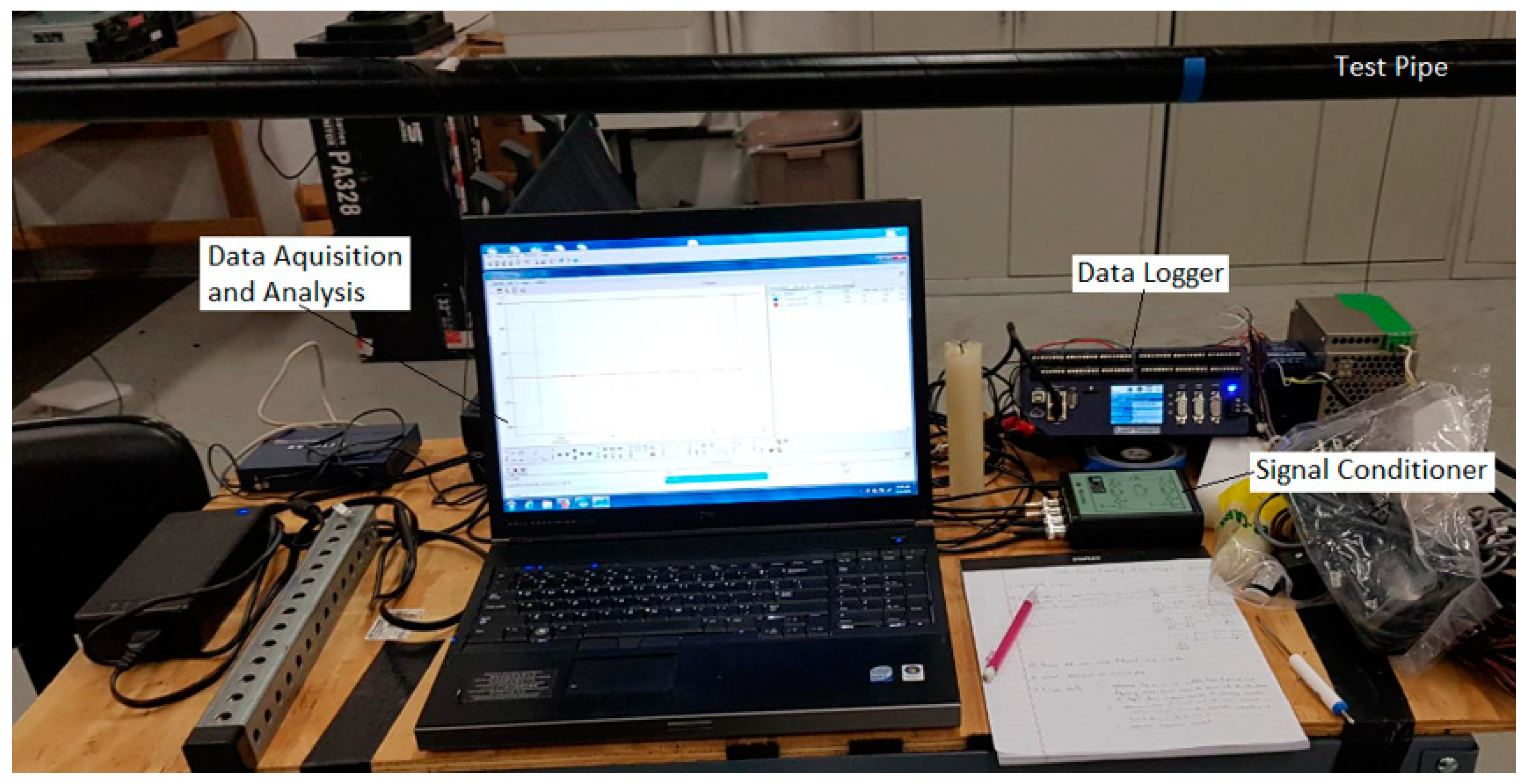
Figure 2.
Sensor placements on test pipe (Locations 1, 2, 3 and 4).
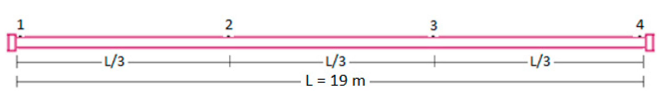
Figure 3.
Calibration and time synchronization of the accelerometers.
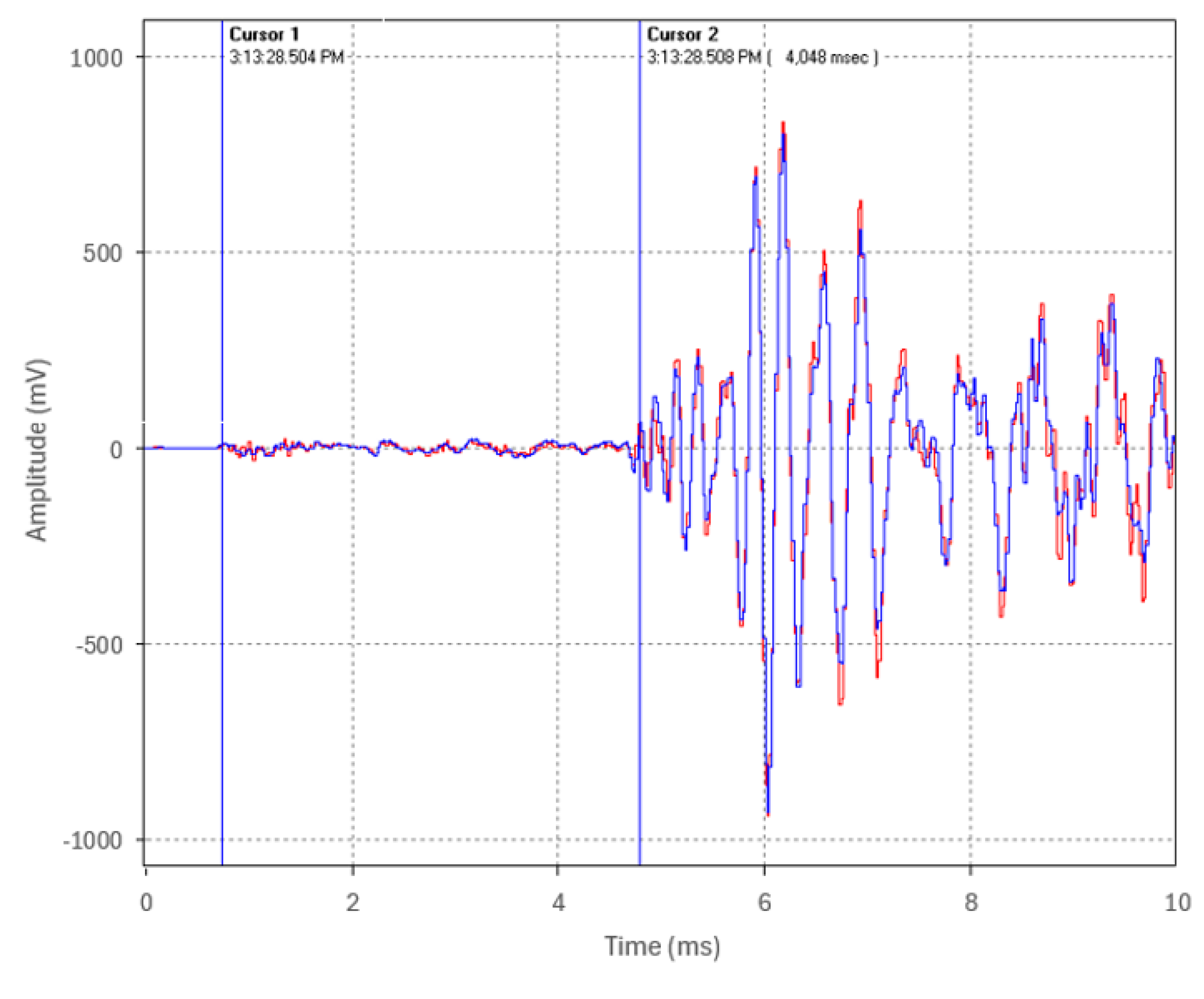
Figure 5.
Fault simulator device connected to surge wave generator.
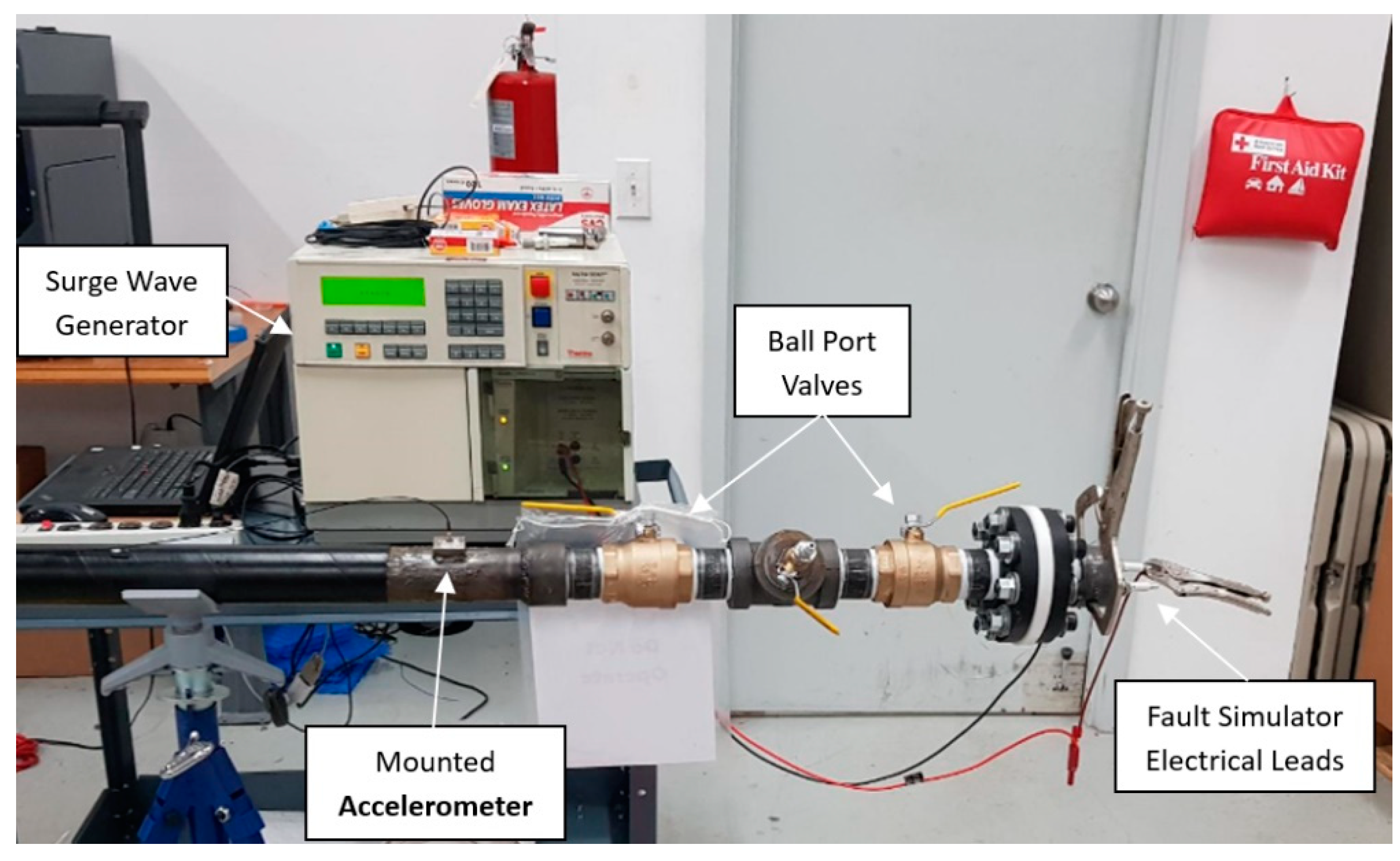
Figure 6.
Pipe supported in air - Test 3.1 configuration.
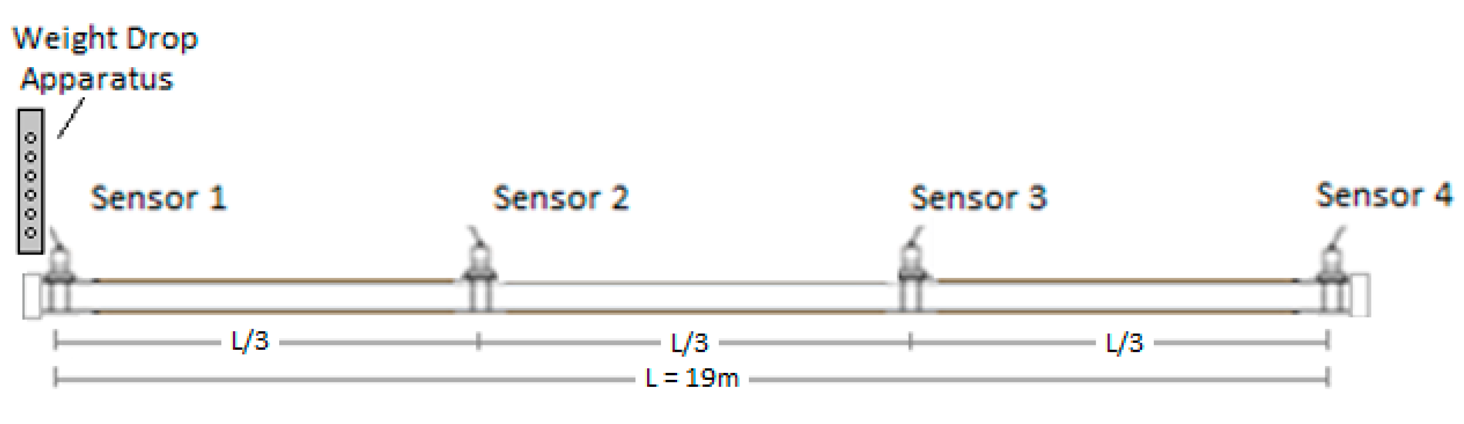
Figure 7.
Test 3.2 Configuration (pipe laid on tamped rock dust) – Impact at Sensor 1 Location.
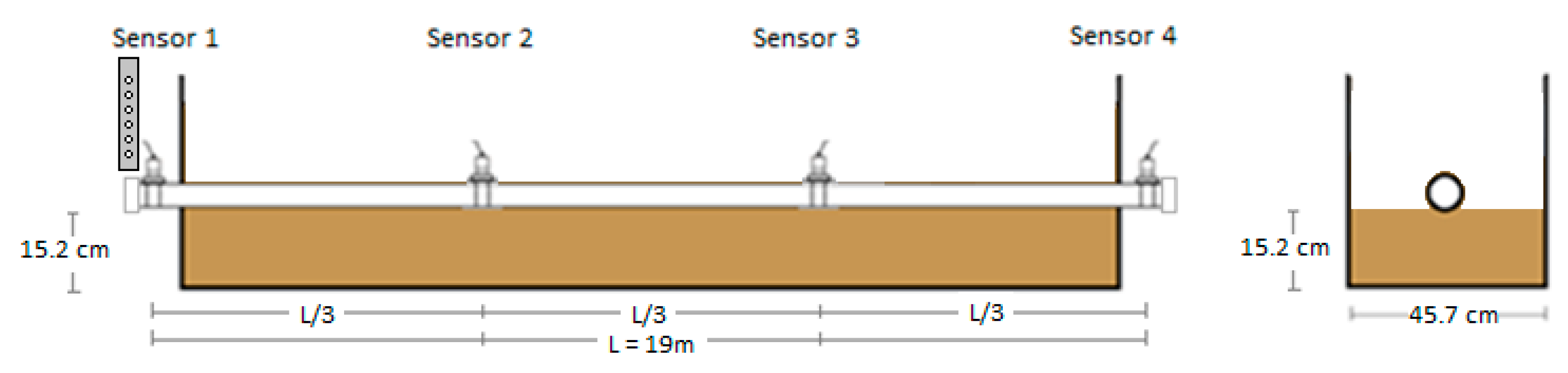
Figure 8.
Tamping and layering process: (a) Rock dust being poured into the containment box; (b) Rock dust tamped in 5–8 cm lifts; (c) Final setup of the pipe laid on 15 cm of tamped rock dust in Test 3.2.
Figure 8.
Tamping and layering process: (a) Rock dust being poured into the containment box; (b) Rock dust tamped in 5–8 cm lifts; (c) Final setup of the pipe laid on 15 cm of tamped rock dust in Test 3.2.
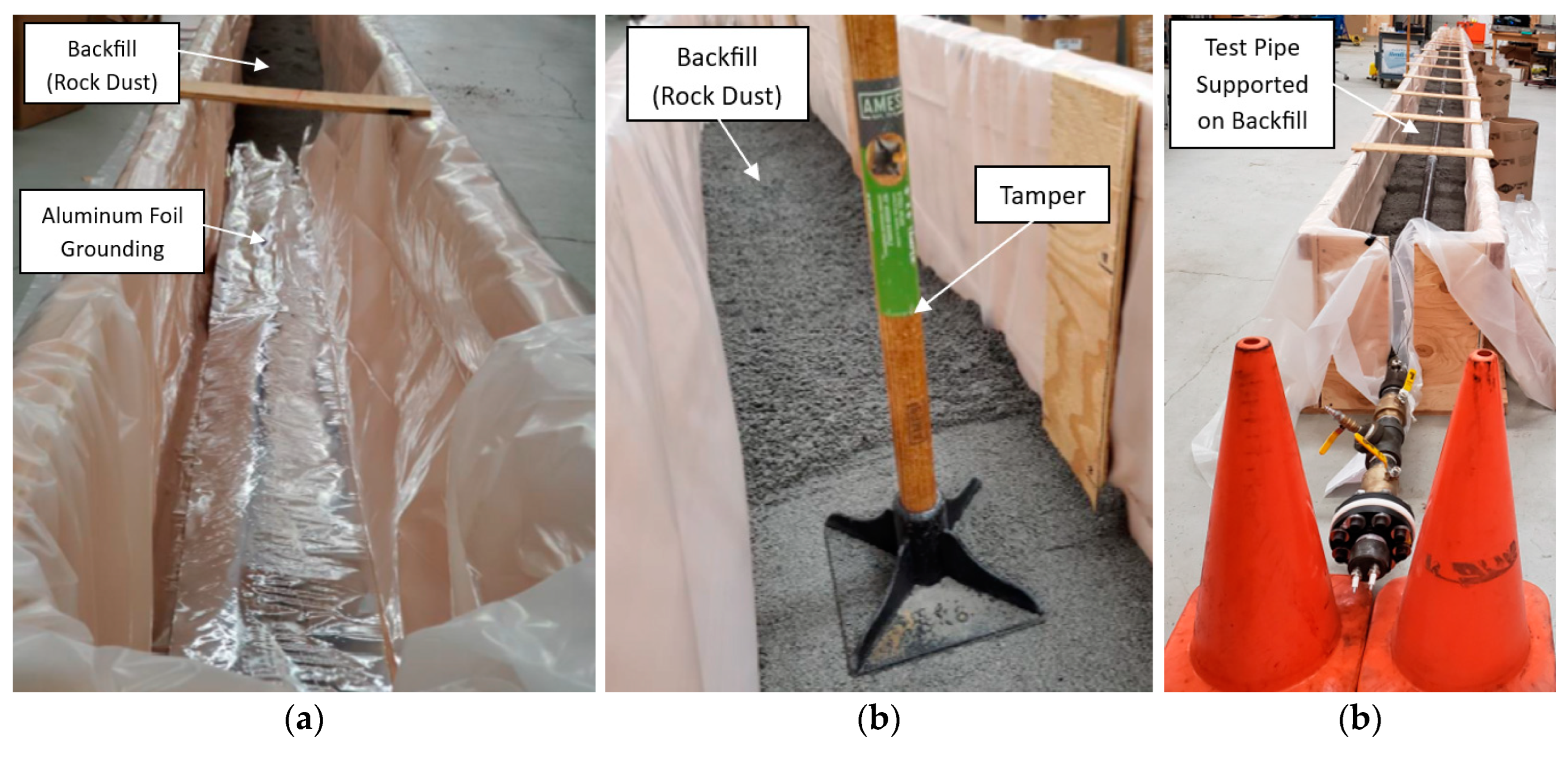
Figure 9.
Test 3.3 Configuration (Fully Embedded) – Impact at Sensor 1 location.
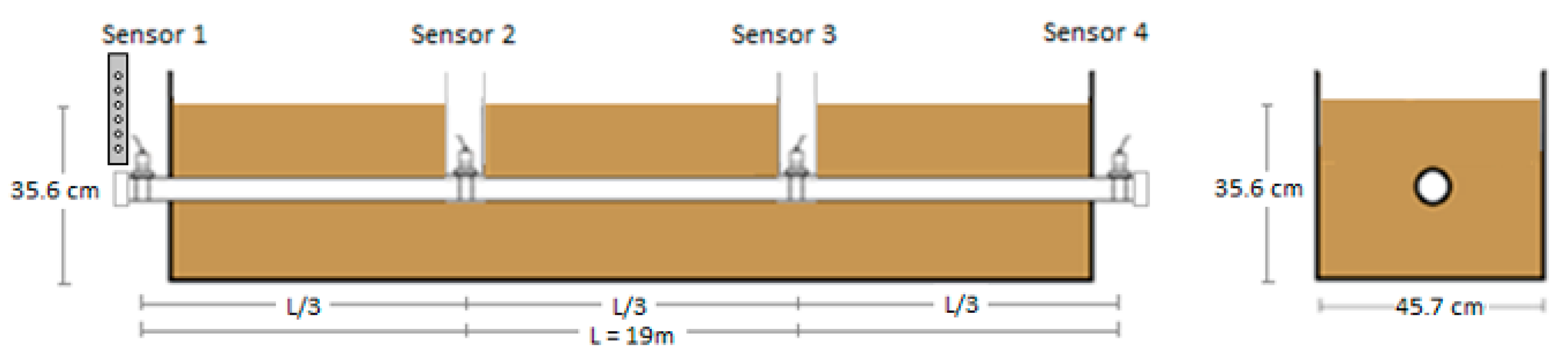
Figure 10.
Test 3.3 - Fully embedded configuration: (a) Complete experimental setup; (b) Manhole access points at intermediate locations for accelerometer placement.
Figure 10.
Test 3.3 - Fully embedded configuration: (a) Complete experimental setup; (b) Manhole access points at intermediate locations for accelerometer placement.
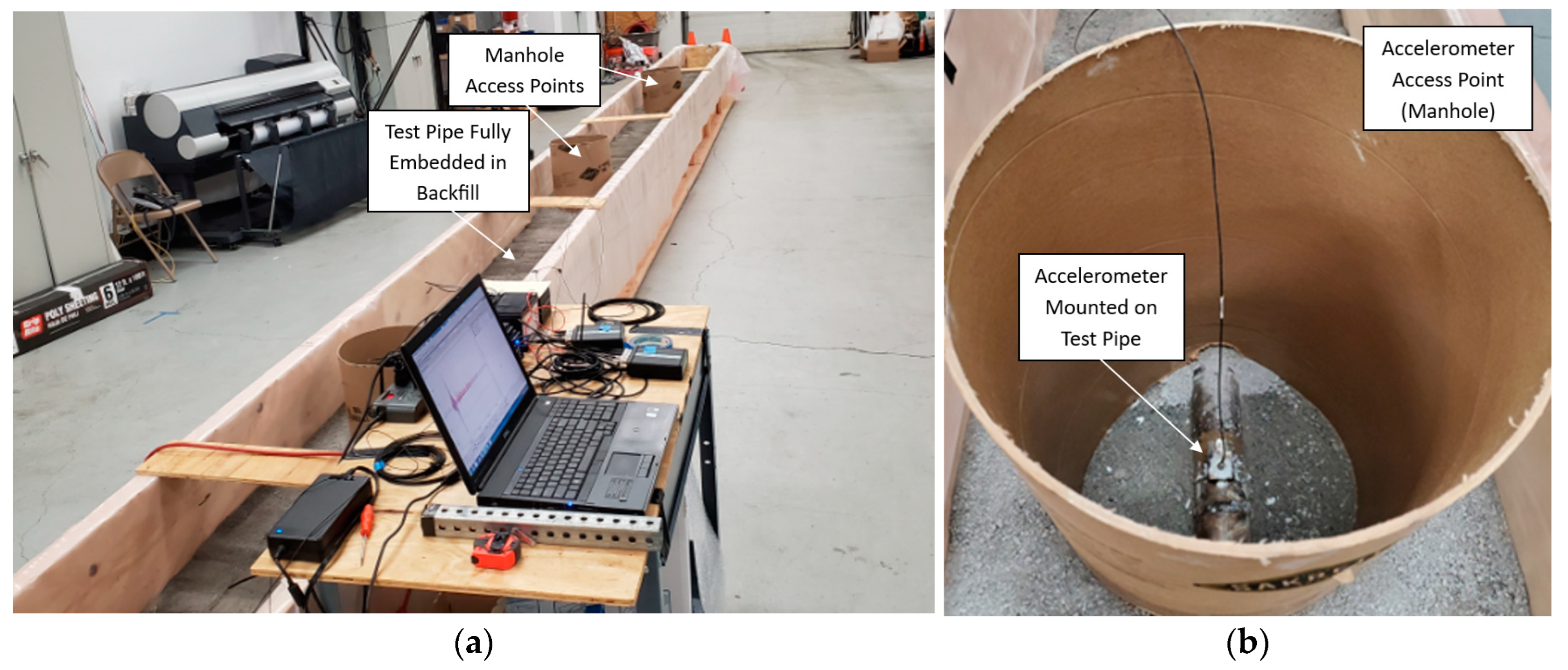
Figure 12.
Acoustic waveforms captured by Sensors 1 and 4 (Test 1.1).
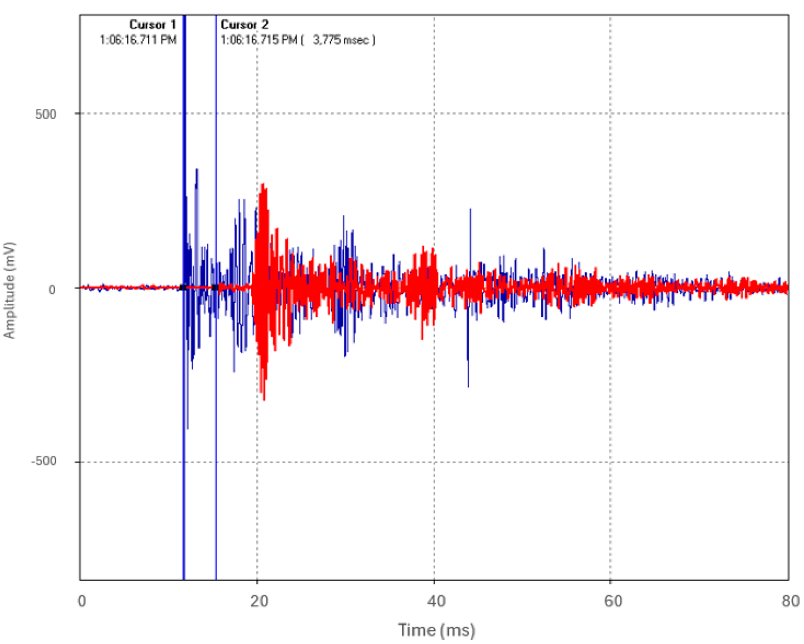
Figure 13.
Close-up snapshot of the timestamping of the acoustic waveforms captured by Sensors 1 and 4 (Test 1.1).
Figure 13.
Close-up snapshot of the timestamping of the acoustic waveforms captured by Sensors 1 and 4 (Test 1.1).
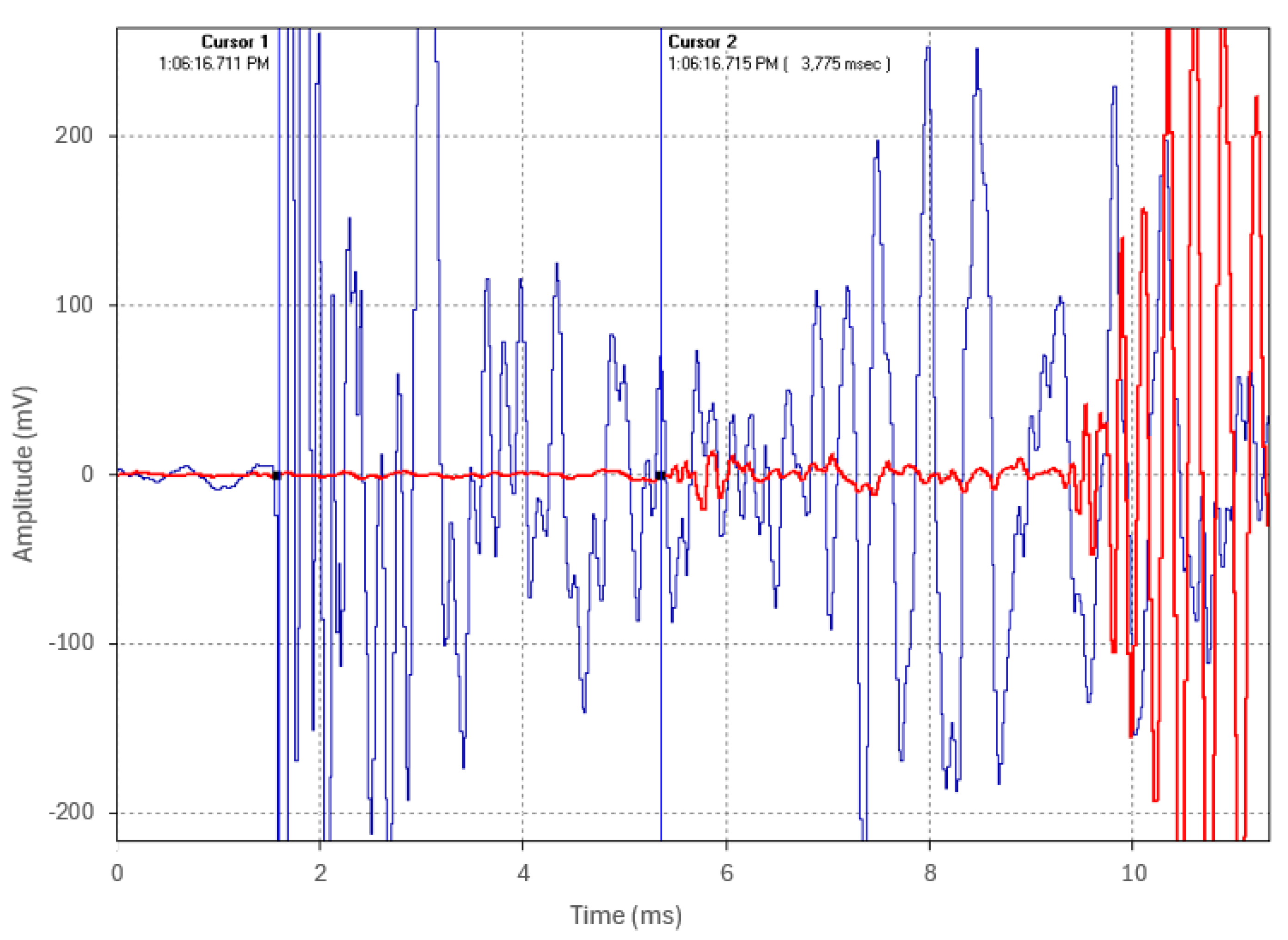
Figure 14.
TDOA of the acoustic pulse at pipe ends when an acoustic pulse is induced at one-third the length of the pipe (Test 1.2).
Figure 14.
TDOA of the acoustic pulse at pipe ends when an acoustic pulse is induced at one-third the length of the pipe (Test 1.2).
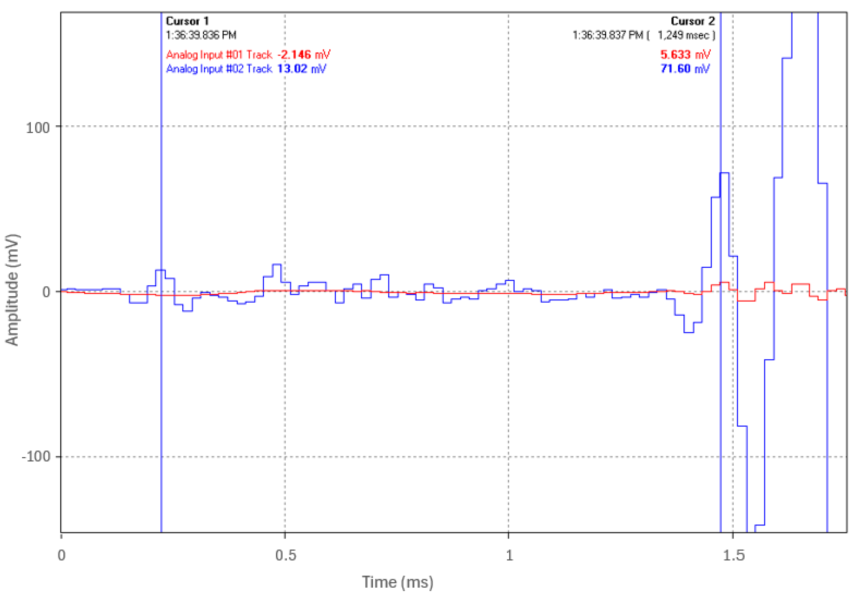
Figure 15.
Test 2 – Blue waveform (Sensor 1); Red waveform (Sensor 4).
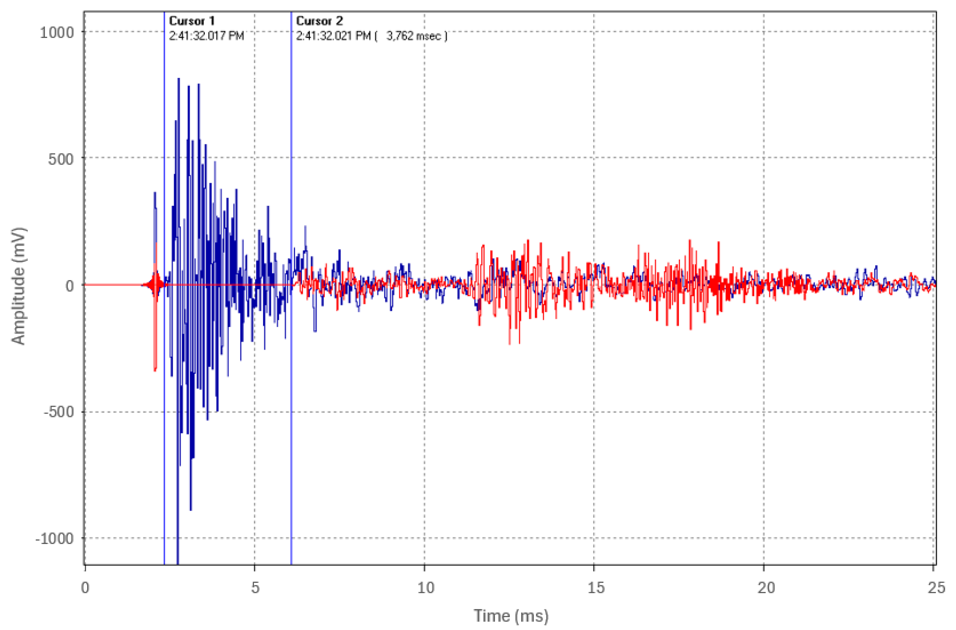
Figure 16.
Overview of peak amplitudes from Sensor 1 for the five test runs of Test 3.1.
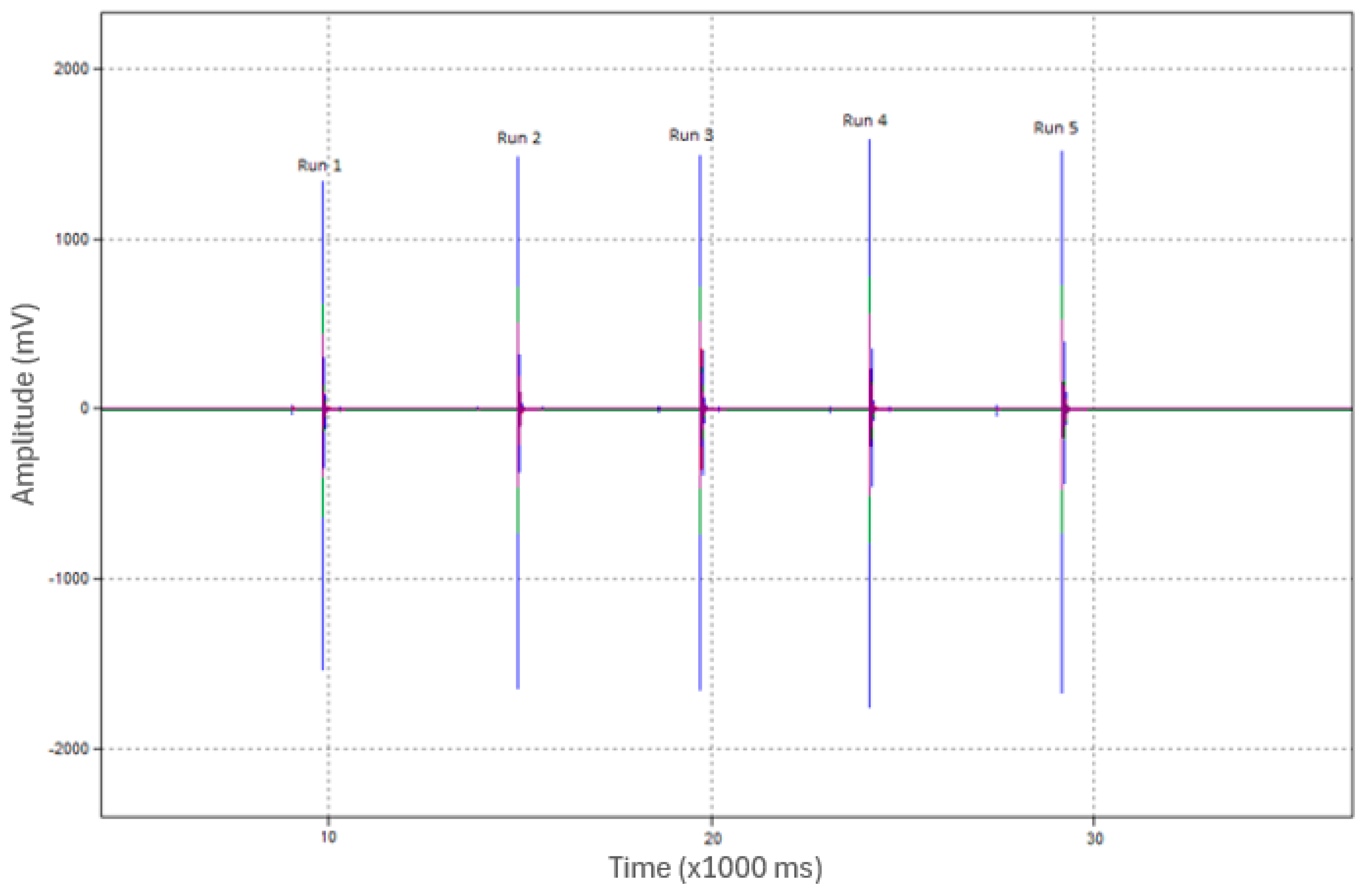
Figure 17.
Captured waveforms from Sensors 1,2,3 and 4 for Run 1 in Test 3.1
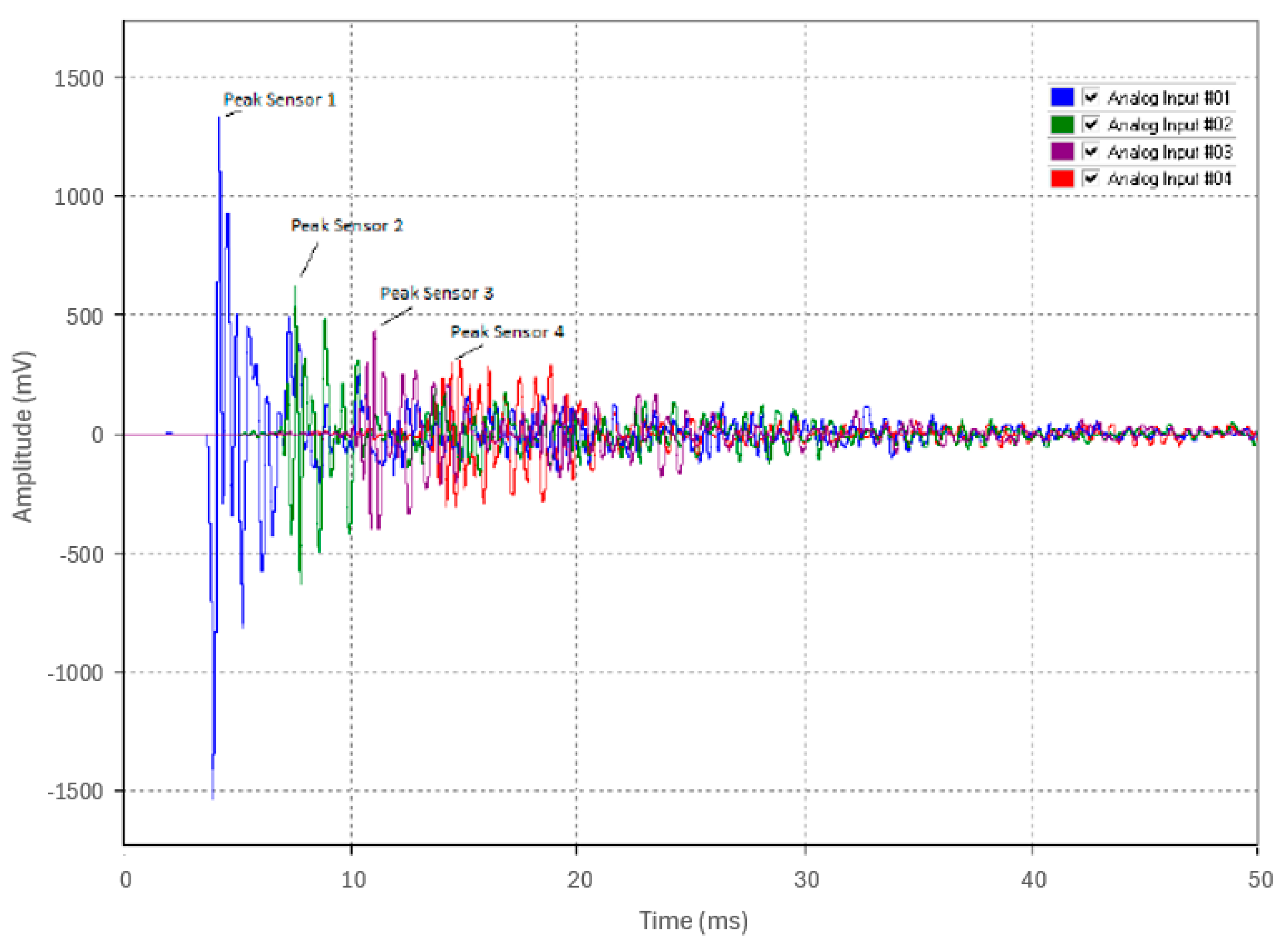
Figure 18.
Acoustic pulse attenuation profile as it propagates along the 19 m pipe in Test 3.1.
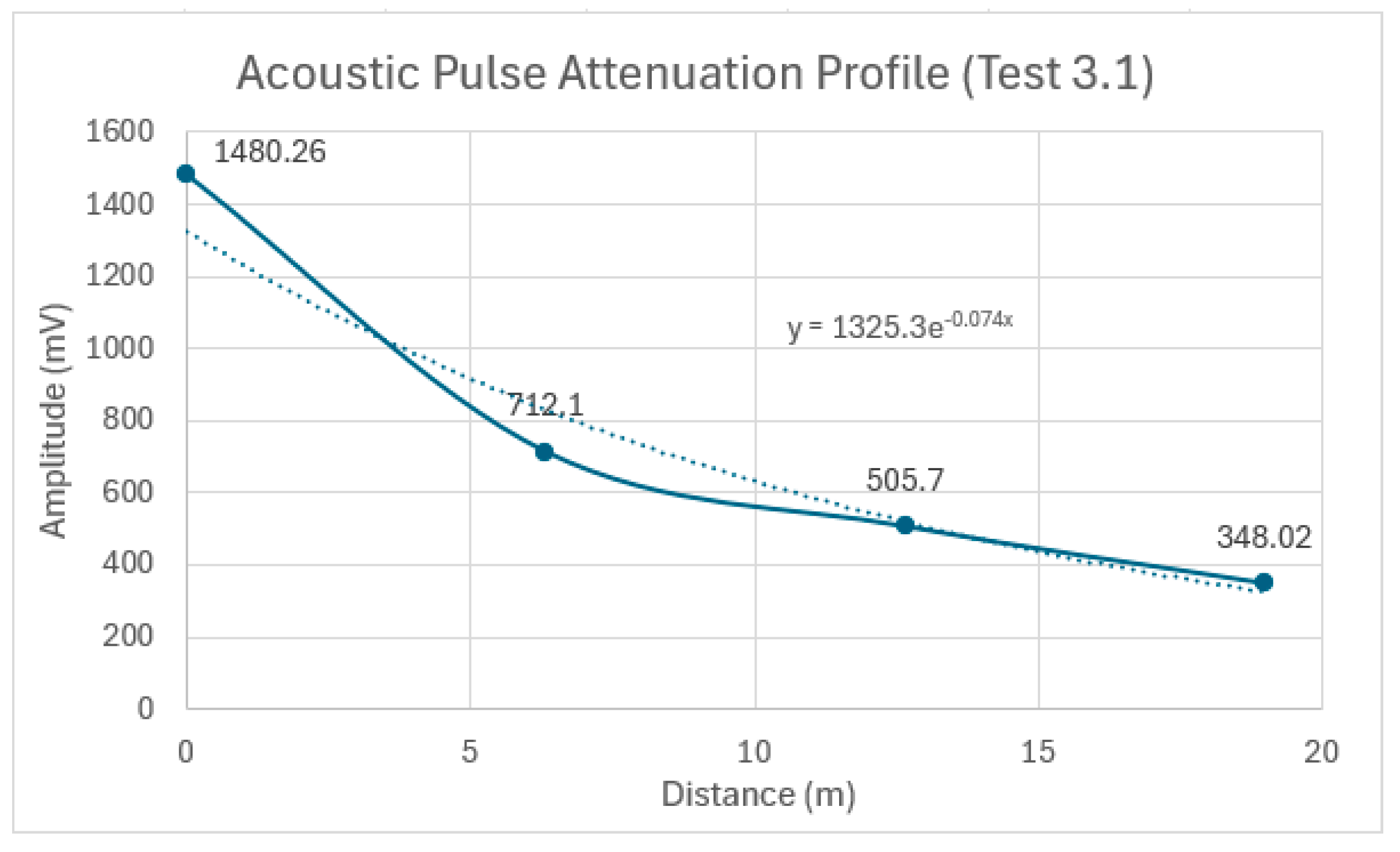
Figure 19.
Waveforms from the four accelerometers of Run 1 in Test 3.2.
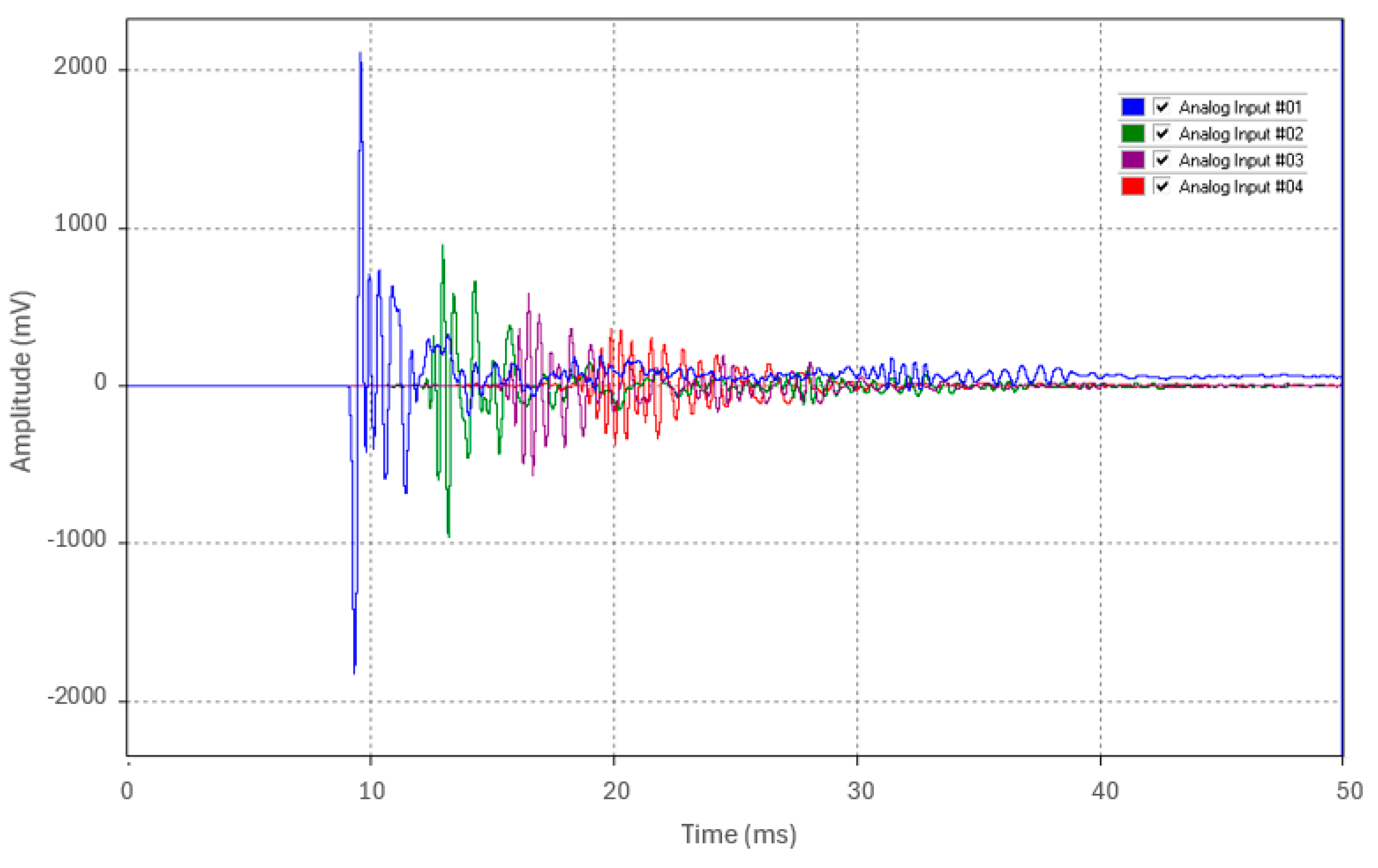
Figure 20.
Acoustic pulse attenuation profile as it propagates along the 19 m pipe in Test 3.2.
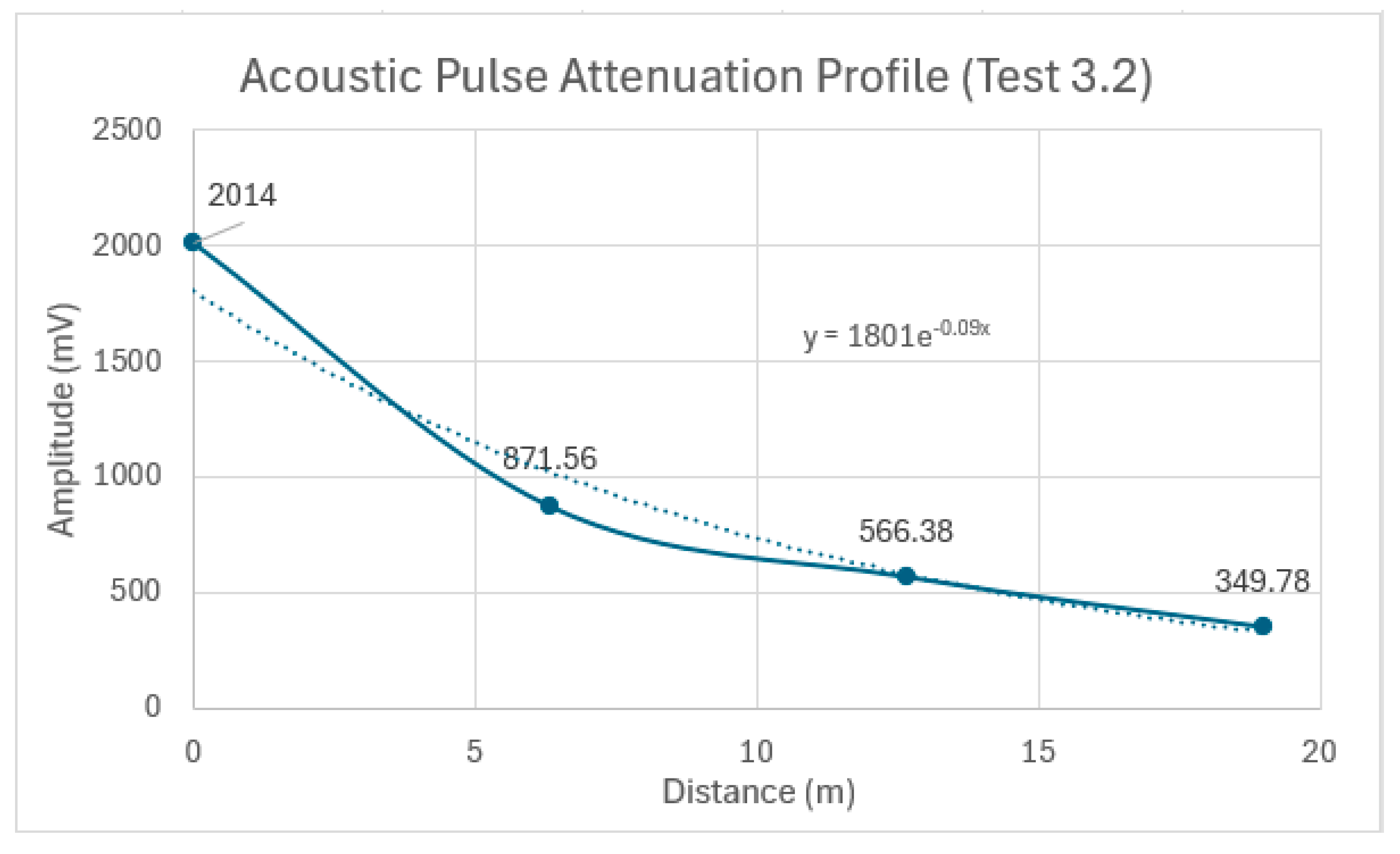
Figure 21.
Waveforms from the four accelerometers of Run 1 in Test 3.3.
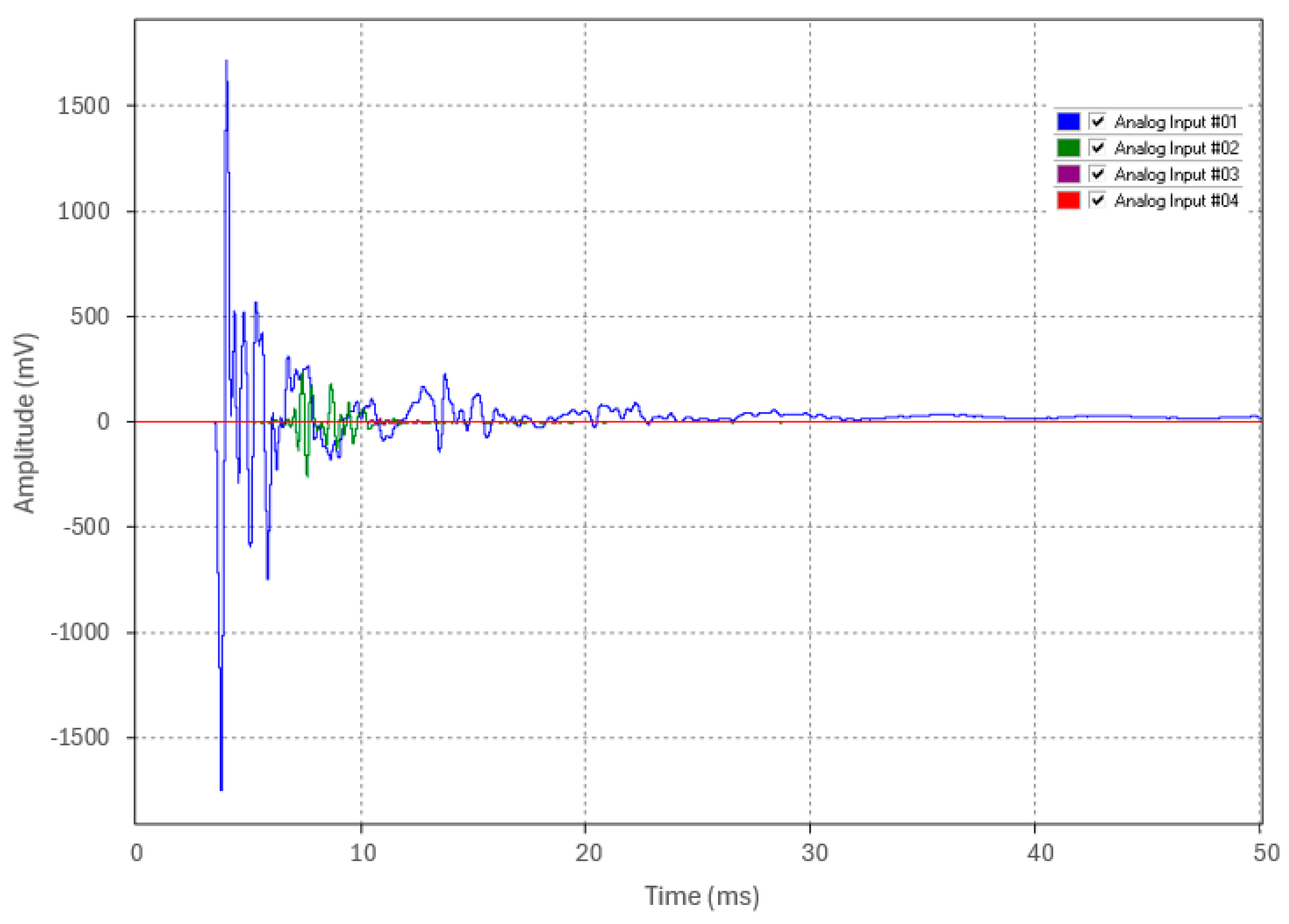
Figure 22.
Acoustic pulse attenuation profile as it propagates along the 19 m pipe in Test 3.2.
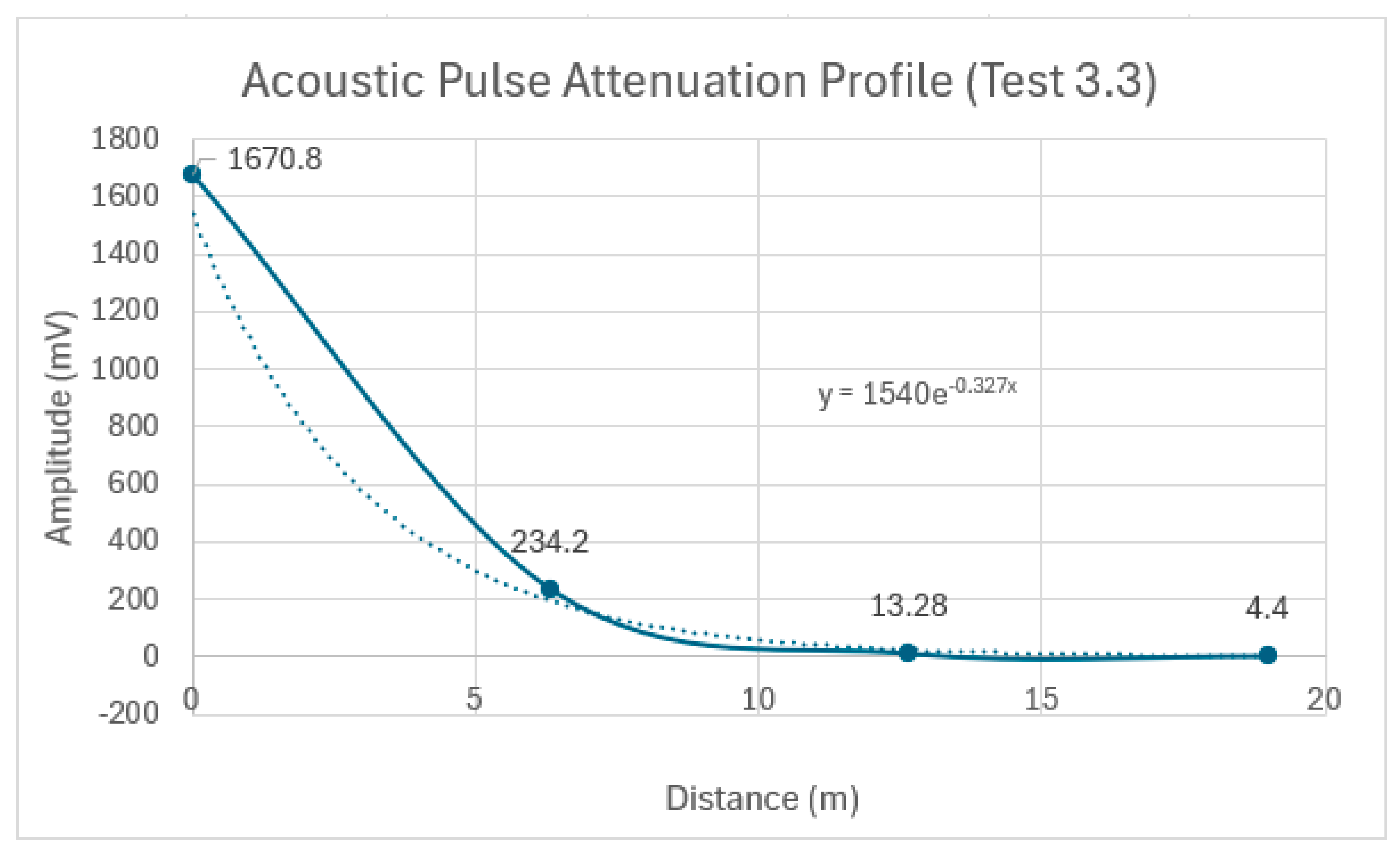
Figure 23.
Fault induced acoustic pulse waveform captured by Sensors 1 and 4 (Test 4)
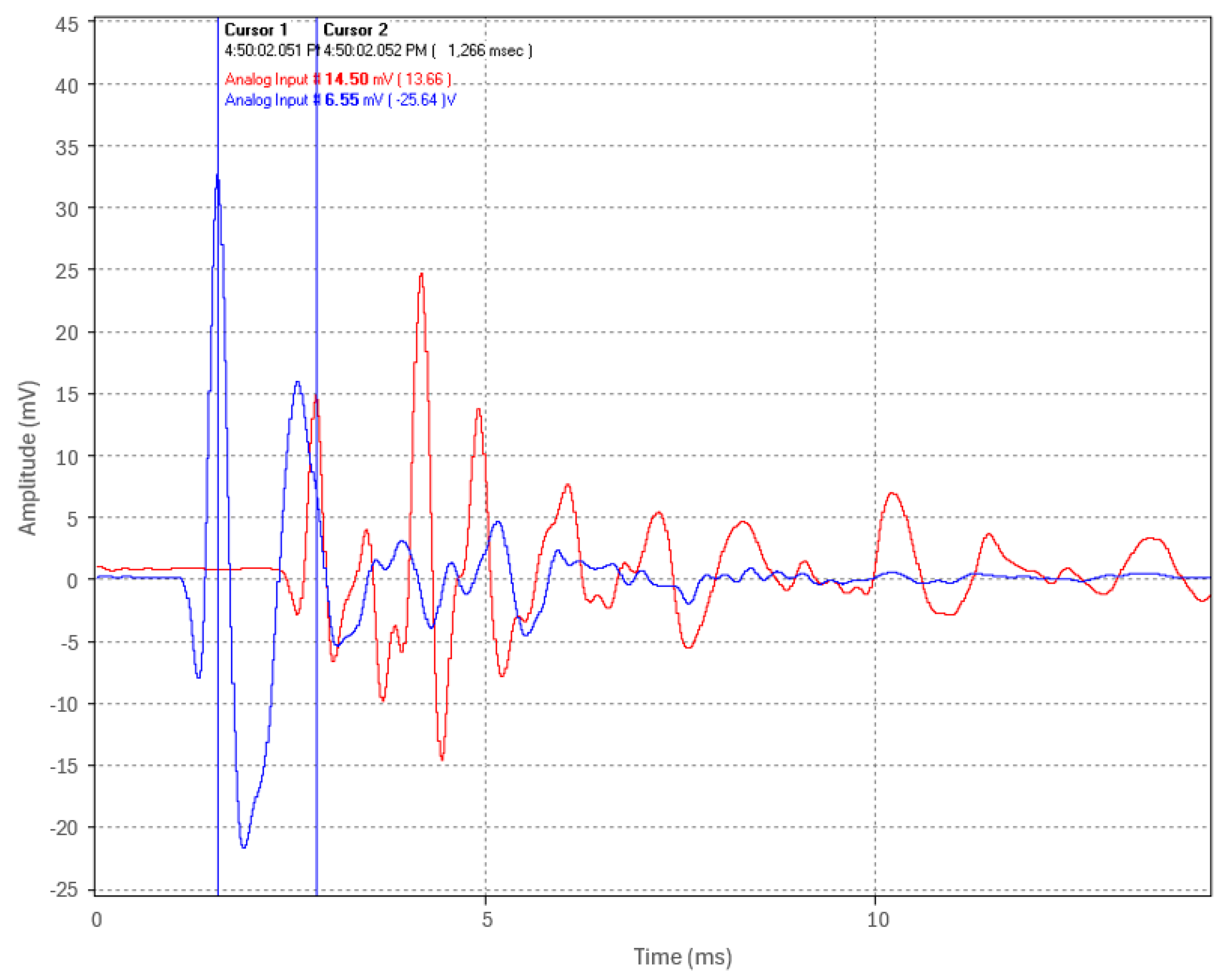
Table 1.
Detailed parameters of the test pipe.
| Item | Value | |
|---|---|---|
| Pipe Length | 19 meters | |
| Material Young's Modulus (E) Density (ρ) Outer Diameter (OD) Inner Diameter (ID) Wall Thickness External Coating Internal Coating |
Carbon Steel 200 GPa 7850 kg/m3 60.33 mm 49.25 mm 5.54 mm (Sch. 80) Pritec Epoxy |
Table 2.
Detailed parameters of the B&K accelerometers.
| Item | Value | |
|---|---|---|
| Product model | B&K 4518-002 | |
| Sensitivity Measurement range Resonant frequency Frequency range Residual Noise Level Maximum Operational Level (peak) Mounting |
10 ±10% mV/g ± 500g 62 kHz 1 – 20000 Hz 2000 µg 500 g Adhesive |
Note: g is the acceleration of gravity.
Table 3.
Detailed parameters of the B&K CCLD signal conditioner.
| Item | Value | |
|---|---|---|
| Product model | B&K 1704-A-002 | |
| Maximum Frequency Minimum Frequency Maximum Gain (dB) Minimum Gain (dB) |
55 kHz 2.2 Hz × 100 (40 dB) × 1 (0 dB) |
Table 3.
Specifications of the Delphin Expert Transient Data Logger.
| Item | Value | |
|---|---|---|
| Product model | Delphin Expert Transient | |
| Number of input channels Number of output channels Voltage range Measurement accuracy Max. input frequency / min. pulse width Sampling rate |
4 8 ± 25 V 0.5 mV + 0.008 % 1 MHz / 500 ns 20 Hz – 50 kHz |
Table 6.
Summary of the experimental tests conducted.
| Test | Objective | Pulse Generation | Embedment Condition | Filter | |
|---|---|---|---|---|---|
| 1.1 | Acoustic velocity | Weight drop, pipe end | In air | 20 kHz LPF | |
| 1.2 | Localization accuracy | Weight drop, 1/3 length | In air | 20 kHz LPF | |
| 2 | Thumping-induced pulse | Fault Simulator, pipe end | In air | 20 kHz LPF | |
| 3.1 | Attenuation in air | Weight drop, 5 reps, pipe end | In air | 3 kHz LPF | |
| 3.2 | Attenuation on backfill | Weight drop, 5 reps, pipe end | On Tamped rock dust | 3 kHz LPF | |
| 3.3 | Attenuation embedded | Weight drop, 5 reps, pipe end | Fully embedded | 3 kHz LPF | |
| 4 | Fault pinpointing | Fault simulator, 1/3 length | Fully embedded | 3 kHz LPF |
Table 7.
Peak amplitudes at each of the four locations (Test 3.2).
| Title 1 Run# | Sensor 1 Peak (mV) | Sensor 2 Peak (mV) | Sensor 2 Peak (mV) | Sensor 2 Peak (mV) |
|---|---|---|---|---|
| 1 2 3 4 5 |
2114 | 892 | 586 | 365.3 |
| 1846 | 852.6 | 550.5 | 344.1 | |
| 1961 2079 2070 |
909.6 848.6 855 |
590.8 553.1 551.5 |
362 339.3 338.2 |
|
| Average | 2014 | 871.6 | 566.4 | 349.8 |
| % Decrease | 56.7% | 35% | 38.2% | |
| Atten. Coefficient | 0.132 Np/m | 0.068 Np/m | 0.076 Np/m |
Table 8.
Peak amplitudes at each of the four sensor locations (Test 3.3).
| Title 1 Run# | Sensor 1 Peak (mV) | Sensor 2 Peak (mV) | Sensor 2 Peak (mV) | Sensor 2 Peak (mV) |
|---|---|---|---|---|
| 1 2 3 4 5 |
1716 | 233 | 13.4 | 4.4 |
| 1630 | 228 | 12.5 | 4.4 | |
| 1663 1683 1662 |
233.2 242.2 234.6 |
13.2 14 13.3 |
4.4 4.7 4.1 |
|
| Average | 1670 | 234.2 | 13.3 | 4.4 |
| % Decrease | 86.0 % | 94.3 % | 66.9 % | |
| Atten. Coefficient | 0.310 Np/m | 0.453 Np/m | 0.174 Np/m |
Disclaimer/Publisher’s Note: The statements, opinions and data contained in all publications are solely those of the individual author(s) and contributor(s) and not of MDPI and/or the editor(s). MDPI and/or the editor(s) disclaim responsibility for any injury to people or property resulting from any ideas, methods, instructions or products referred to in the content. |
© 2024 by the authors. Licensee MDPI, Basel, Switzerland. This article is an open access article distributed under the terms and conditions of the Creative Commons Attribution (CC BY) license (http://creativecommons.org/licenses/by/4.0/).
Copyright: This open access article is published under a Creative Commons CC BY 4.0 license, which permit the free download, distribution, and reuse, provided that the author and preprint are cited in any reuse.


