
Submitted:
18 November 2025
Posted:
27 November 2025
You are already at the latest version
Abstract
We formulate a single, sector–neutral Lyapunov law that treats quantum mechanics, thermodynamics, and general relativity as three calibrations of one underlying feedback structure. The basic data are a shared Hilbert space, a blueprint space of statistical degrees of freedom, a physical space of realised degrees of freedom, and a calibration map between them. Their mismatch is quantified by one quadratic residual of sameness in a fixed instrument norm. Admissible evolutions are those that preserve calibration and are nonexpansive in this norm; for such evolutions we prove a data–processing inequality for the residual, a Lyapunov inequality with an intrinsic DSFL clock, and a cone–type locality condition. We then build explicit quantum, thermodynamic, and gravitational calibrations and show that their sectoral residuals add to a single global residual whose decay rate is controlled by the slowest sector. In this picture, collapse, entropy production, and curvature–matter balance become three faces of the same residual–driven attractor. A UV master inequality explains how scale–resolved models fit into one global DSFL law, and simple model worlds (qubit channels, Markov chains, QNM–like modes, and a Bell/CHSH sector) illustrate how standard phenomena such as Born statistics, ringdown, and Tsirelson–saturating nonlocality can all be read as structural consequences of one calibrated residual in one Hilbert space.
Keywords:
Deterministic Statistical Feedback Law
; residual of sameness
; single calibrated Hilbert space
; Lyapunov law and DSFL clock
; quantum collapse and Born rule
; Markov chains and χ2–divergence
; Einstein imbalance and quasinormal modes
; UV master inequality
; asymptotic Rsameness gap
; structural quantum gravity
Notation (Symbols Only)
| Symbol | Type / Domain | Meaning / Assumptions |
| Ambient Hilbert geometry (“one room”) | ||
| Hilbert space | Common comparison space with inner product and norm | |
| Closed subspaces | Statistical (blueprint, sDoF) and physical (response, pDoF) arenas | |
| Closed subspaces | Alternative notation for (sector–neutral definitions) | |
| Projections | Orthogonal projectors onto , in the ambient inner product | |
| Linear map | Calibration / interchangeability map (blueprint → ideal response) | |
| Closed subspace | Coherent image of on the physical side (after closure) | |
| Projection | Orthogonal projector onto U | |
| SPD operator | Instrument weight; induces instrument inner product and norm | |
| Norm | Instrument norm on , associated with W | |
| States, channels, duals | ||
| Hilbert space | Finite–dimensional quantum system, typically | |
| Operator space | Matrices / bounded operators on | |
| State space | Density matrices with | |
| Operators | Quantum states in | |
| Linear map | Quantum channel (CPTP) or general linear update on | |
| Linear map | Blueprint update on ; DSFL pair is | |
| Linear map | Hilbert–Schmidt adjoint of | |
| Operator norm | Induced norm ; DSFL admissibility requires | |
| Operators | Kraus operators of a CPTP channel, | |
| Operator on | Gram operator ; controls via its largest eigenvalue | |
| Scalar | Largest eigenvalue of ; equals in finite dimension | |
| Scalar | DSFL gap | |
| Residual of sameness and defects | ||
| Vector | Statistical (blueprint, sDoF) state | |
| Vector | Physical (response, pDoF) state | |
| Vector in | Calibrated mismatch (defect, residual direction) | |
| , | Scalar | Residual of sameness: |
| Scalar | Generic notation for a DSFL residual (when no sector is specified) | |
| Nonnegative scalar | Residual magnitude, e.g. half–width in DSFL band tests | |
| Scalar | Total residual in a block–diagonal room (QM+TD+GR toy) | |
| Scalars | Sectoral residuals in QM, TD and GR calibrations | |
| Scalar | Correlation residual (inside–outside or bipartite) | |
| Frames, projectors, angles | ||
| Closed subspace | Measurement / reconstruction / constraint frame | |
| Projection | Orthogonal projector onto V (ambient inner product) | |
| Closed subspace | Spectral frame of observable A (after graph transport) | |
| Angle | Friedrichs angle; | |
| Scalar in | Overlap constant | |
| Closed subspace | Closed linear span of two frames , | |
| Variance and graph transport (when used) | ||
| Operator | Centered observable: | |
| Isomorphism | Graph–norm isomorphism | |
| Closed subspace | A–frame in after graph transport | |
| Nonnegative scalar | Standard deviation: | |
| Admissibility, DPI, and operators | ||
| Linear map | Statistical update (blueprint side) | |
| Linear map | Physical update (response side) | |
| Identity | Intertwining (coherent blueprint → coherent response) | |
| Operator inequality | Spectral DPI / nonexpansiveness in | |
| DSFL–admissible | Property | and (equivalently DPI for R) |
| Inequality | Data–processing inequality for the single observable R | |
| Two–loop dynamics and DSFL time | ||
| Trajectory in | Time–dependent residual | |
| Operator on | Immediate loop generator; selfadjoint, | |
| Operator kernel | Retarded, Loewner–positive memory kernel for | |
| Vector in | Remainder; | |
| Nonnegative scalar | Coercivity bound: | |
| Nonnegative scalar | Remainder bound in the Lyapunov inequality | |
| Nonnegative scalar | Instantaneous decay rate (envelope rate) | |
| Nonnegative scalar | Residual energy in time | |
| Scalar | DSFL time via ; unit–slope Lyapunov clock | |
| Nonnegative scalars | Sectoral Lyapunov rates in QM, TD, GR calibrations | |
| Causality and cone parameters (relay loop) | ||
| c | Speed constant | Instrument light–cone speed (cone front speed) |
| Semigroup on | Relay evolution; cone bound with margin | |
| Projection/localiser | Projection onto defects supported in region O | |
| Length/time scale | Cone sharpness in bounds of the form | |
| Cutoff | Ultraviolet regulator; typically | |
| Finite–dimensional quantum sector | ||
| Hilbert spaces | Local qubit / qudit spaces, typically , | |
| Hilbert space | Tensor product | |
| Density matrix | Bipartite state on | |
| Density matrices | Reduced states: , | |
| Density matrix | Bell state in the two–qubit sector | |
| Partial transpose | Transposition on subsystem B in a fixed basis | |
| Entanglement and correlation proxies | ||
| Scalar | Negativity: | |
| Scalar | Sandwiched Rényi divergence to product form | |
| Scalar | Trace distance to product: | |
| Scalar | DSFL correlation residual | |
| Bell / CHSH notation | ||
| Observables | Local dichotomic () observables on | |
| Observables | Local dichotomic () observables on | |
| C | Operator | CHSH operator |
| Scalar | CHSH value | |
| Scalar | Classical (local hidden–variable) CHSH value; | |
| Scalar | DSFL / quantum CHSH value; (Tsirelson bound) | |
| Thermodynamic and GR model worlds | ||
| L | Generator | Markov generator on a finite state space (TD block) |
| Probability vector | Classical distribution at time t; stationary distribution | |
| Scalar | TD residual | |
| Tensor | Einstein imbalance (GR toy) | |
| Scalar | GR residual | |
| Scalar | DSFL rate in GR toy, controlled by dominant quasi–normal modes | |
| Global / UV DSFL quantities | ||
| Scalar | Scale–resolved sectoral residual in sector at cutoff | |
| Scalar | Scale–resolved global residual | |
| Scalar | UV–limit sectoral residual in sector | |
| Scalar | UV–limit global residual | |
| Scalar | Scale–resolved DSFL rate in sector a at cutoff | |
| Scalar | UV–limit DSFL rate in sector a | |
| Scalar | Slowest sectoral rate at scale , | |
| Scalar | UV–limit slowest rate, | |
| Scalar | UV / global DSFL time: | |
| Scalar | Asymptotic Rsameness gap: (when it exists) | |
| Scalar | de Sitter / Kerr–de Sitter gap; positive QNM / energy–decay scale in GR models | |
| Scalar | Microscopic DSFL gap in a PPE–SABIM–gravity room (QG appendix) | |
| Sector label | Optional quantum–geometric sector in extended four–sector DSFL constructions | |
| Scrambling, Page time, and complexity | ||
| Scalar | DSFL scrambling time: minimal time/steps to reduce a residual by factor | |
| Scalar | DSFL Page–like time (inside/outside DSFL residuals equal, correlation residual peaked) | |
| Scalar | DSFL Lyapunov rate in simple toy models, | |
| Scalar | Entropy–response exponent, e.g. in the toy Page law | |
| Scalar | DSFL depth / complexity (Lyapunov depth or cumulative DSFL time) | |
| Scalar | Computational complexity (when used in conditional Susskind–type bounds) | |
| Scalar | Chaos / Lyapunov exponent in MSS OTOC bound[1] | |
| Scalar | Inverse temperature, | |
| Miscellaneous symbols | ||
| Norm | Ambient norm (context may indicate operator, Hilbert–Schmidt, or trace norm) | |
| Inner product | Ambient inner product | |
| Loewner order | Positive semidefinite operator: for all x | |
| Nonnegative scalar | Distance of x to subspace V in | |
1. Introduction
The standard formulation of fundamental physics assigns different state spaces, metrics, and arrows of time to quantum mechanics (QM), thermodynamics (TD), and general relativity (GR). Quantum states live in Hilbert spaces and operator algebras; thermodynamic states in spaces of probability measures or density matrices equipped with entropy functionals; gravitational states in spaces of Lorentzian metrics and stress–energy tensors constrained by the Einstein equations. Their equilibrium principles are encoded in different objects: Born’s rule and stationary density matrices in QM, entropy maximisation and detailed balance in TD, and the curvature–matter balance in GR (e.g. [2,3,4,5,6,7,8,9,10]). In the usual presentation these are taken as sector–specific postulates: the Born probabilities for measurement outcomes in QM, the maximisation of entropy under constraints in TD, and the Einstein equations and their attractor geometries in GR.
The aim of this paper is to show that these sector–specific formulations can be recast as three calibrations of a single, more elementary structure: a common Hilbert space equipped with a quadratic residual that quantifies how far a realised configuration of physical degrees of freedom deviates from a calibrated statistical blueprint. This residual plays the rôle of a Lyapunov function for a class of admissible evolutions and defines what we call the Deterministic Statistical Feedback Law (DSFL). Concretely, we work with a Hilbert space carrying two closed subspaces and of statistical (sDoF, “blueprints”) and physical (pDoF, “responses”) degrees of freedom, a bounded calibration map , and a strictly positive, selfadjoint instrument weight . The elementary scalar observable is the residual of sameness
where , , and defines the instrument norm.
The conceptual move is to declare that, at the DSFL level, this single observable is the only quantity with dynamical status. All sectoral objects that usually play the rôle of equilibrium measures or “arrows of time”—Born weights in QM, entropy functionals and spectral gaps in TD, and curvature–matter imbalance and quasi–normal–mode rates in GR—are read as specific ways of embedding their data into the common room and then inspecting the behaviour of the same quadratic mismatch. In other words, we do not postulate different entropies or Lyapunov functionals in different sectors; instead, we insist that all of them arise as shadows or calibrations of a single residual in one geometry.
Admissible evolutions in this geometry are those that preserve calibration (intertwine on the blueprint and response sides) and are nonexpansive in . For such evolutions we prove three structural statements: (i) a data–processing inequality (DPI) for the single observable , (ii) a Lyapunov inequality
for some rate function , and (iii) a cone–type locality condition that encodes finite–speed propagation in the same instrument norm, in the spirit of Lieb–Robinson bounds.[11,12,13,14] The Lyapunov inequality induces an intrinsic DSFL time in which lies on or below a straight line of slope , as in abstract semigroup theory and stability analysis.[15,16] Thus, once a calibration is fixed, the DSFL layer provides a canonical “clock” and a canonical notion of depth, independent of microscopic details.
Conceptually, the DSFL viewpoint separates three rôles that are usually intertwined:
- Blueprints encode conditional statistics or target configurations (wave functions, probability measures, geometric data). They live in and need not carry their own dynamics; they say what an instrument is aiming to realise.
- Physical responses encode what an instrument or device actually outputs. They live in and are evaluated in a fixed instrument norm induced by W; they capture what is really delivered by the dynamics or measurement.
- Calibration is the deterministic map that realises blueprints as responses. The residual of sameness is the squared norm of this calibration mismatch and is the only scalar DSFL observable we use to talk about approach to equilibrium, contractivity, or locality.
In this light familiar equilibrium, principles become statements of the form “the residual vanishes in a given calibration” (for instance, for a stationary state, or for an Einstein solution), and irreversibility becomes the statement that admissible evolutions contract the residual in a fixed norm. Entropic and geometric functionals are no longer independent axioms in each sector, but appear as sector–specific manifestations of a single quadratic Lyapunov functional. In the remainder of the paper we make this precise by constructing sectoral rooms for QM, TD and GR, proving Lyapunov and cone bounds in each, and then combining them into a single multi–sector residual whose decay is governed by the slowest sector.
Quantum information theory provides a natural starting point. It offers a rich toolkit of functionals and inequalities: contractive channels, relative entropies and sandwiched Rényi divergences, entanglement monotones, and Lyapunov/entropy functionals for quantum Markov semigroups [2,3,4,5,8,17,18]. Classical and quantum statistical mechanics use spectral gaps, Poincaré and logarithmic Sobolev inequalities, and Wasserstein–type distances to quantify mixing and entropy production [6,7,8,19]. On the gravitational side, black–hole spacetimes and cosmological backgrounds carry their own notions of relaxation: quasi–normal–mode ringdown, horizon thermodynamics, and semiclassical backreaction [9,10,20,21,22,23,24]. These tools are usually treated as distinct, each living in its own state space and metric, each with its own data–processing principle. Even in holographic contexts, where bulk gravity is encoded in a boundary quantum theory [25,26,27], the arrows of time in QM, TD and GR are typically discussed in sector–specific languages (entanglement wedges, thermalisation, quasi–normal–mode decay, chaos bounds [1,28,29]).
A natural question is whether there is a single geometric object that can organise all of these as different calibrations of the same underlying structure: one comparison space, one residual, one notion of admissible dynamics and one intrinsic time parameter. The DSFL framework, developed in Section 2, is designed precisely for this purpose. In the present paper we apply it simultaneously to QM, TD and GR in a class of finite–dimensional and linearised model worlds, and construct sectoral DSFL calibrations in which collapse, entropy production, and curvature–matter balance all arise as instances of the same residual–driven attractor. A unification theorem shows that these sectoral residuals add to a single global residual whose decay rate is controlled by the slowest sector. A UV master inequality then explains how scale–resolved models at finite cutoff fit into one global DSFL law, and explicit model worlds (qubit channels, Markov chains, and QNM–like modes) serve as analytic stress tests of the Lyapunov and locality predictions.
2. Sector–Neutral DSFL Framework
The Deterministic Statistical Feedback Law (DSFL) is designed to replace sector–specific equilibrium and irreversibility postulates (Born’s rule in QM, entropy principles in TD, Einstein balance in GR) by a single Hilbert–space structure equipped with:
- a calibrated room in which statistical blueprints and physical responses live side by side;
- a residual of sameness that measures calibration mismatch;
In this section we define these objects and state the key structural results. Proofs and further functional–analytic detail are deferred to Appendix H. The same sector–neutral DSFL machinery will later be used twice: first to unify QM, TD and GR model sectors in one room (Section 3.4), and then, in a companion construction, to formulate a structural notion of quantum gravity as a microscopic completion of the single residual law (cf. Section 2.1).
2.1. Structural Quantum Gravity
Throughout this paper, “quantum gravity” is understood in a structural rather than model–specific sense. We do not propose a particular microscopic theory of geometry; instead, we ask what it means for any microscopic quantum theory to complete the three–sector DSFL loop.
In DSFL language, a quantum–gravitational completion is a microscopic DSFL room with a genuine contraction gap and a family of DSFL–admissible coarse–grainings into the quantum (QM), thermodynamic (TD) and geometric (GR) calibrations. The only primitive scalar is the microscopic residual of sameness, and “gravity” appears as an emergent slow sector in the global residual of sameness, constrained by a UV master DSFL law and by comparison with geometric (de Sitter / QNM) gaps.
Section B and Appendix A.3 make this precise: a DSFL quantum–gravity model is defined “backwards” as any microscopic DSFL room whose residual contracts with a gap, and whose coarse–grainings into QM, TD and GR sectors satisfy the UV master inequality and the emergent–gravity conditions of Theorems 1 and A4. The present subsection only fixes this structural viewpoint; all detailed assumptions are collected later in the dedicated quantum–gravity sections.
2.2. Room, Calibration, and Residual
We start from a fixed Hilbert space , which serves as the common comparison geometry for all sectors (QM, TD, GR).[15,16] The basic ingredients are collected in the following definition.
Definition 1
(DSFL room and residual of sameness). A DSFL room consists of:
- a Hilbert space ;
- a closed subspace of statistical degrees of freedom (sDoF, “blueprints”);
- a closed subspace of physical degrees of freedom (pDoF, “responses”);
- a bounded linear calibration map ;
- a bounded, selfadjoint, strictly positive instrument weight , inducing the inner product and norm
Given and , the DSFL defect and residual of sameness are
Theorem 1
(Positivity and zero set of the residual). In any DSFL room,
- (a)
- for all ;
- (b)
- if and only if .
Equivalently, the zero set of R is exactly the calibration graph
Remark 1
(A single quantitative observable). The scalar is theonlydynamical observable built into the DSFL framework. In later sections we show that Born probabilities in QM, entropy production in TD, and Einstein balance in GR can all be phrased as statements about the vanishing or decay of this single residual in different calibrations of the same room. In the multi–sector setting of Section 3.4, and in UV limits with scale–dependent weights and rates (Appendix A), R becomes a global residual of sameness whose Lyapunov envelope controls all sectors simultaneously.
2.3. Admissible Maps and a Residual Data–Processing Inequality
We now formalise which evolutions on are deemed “lawful” from the DSFL viewpoint.
Definition 2
(DSFL–admissible pair). Let be a DSFL room. A pair of bounded linear maps
is DSFL–admissible if
- (a)
- (calibration preservation)
- (b)
- (nonexpansiveness in the instrument norm)
Theorem 2
(Admissibility ⟺ DPI for R). In a DSFL room, let be bounded linear maps as above. Then the following are equivalent:
- (i)
- is DSFL–admissible;
- (ii)
- for all one has the residual data–processing inequality
In finite dimension, nonexpansiveness is equivalent to a simple spectral condition on a Gram–type operator.
Definition 3
(Gram operator and DSFL gap). Let be bounded and . The Gram operator of Φ in the instrument geometry is
and the induced operator norm is
The DSFL gap of Φ is
Lemma 1
Remark 2
(From one–step DPI to global master laws). At this level, DSFL admissibility is a purely geometric condition on Φ and W. In later sections we iterate such maps across sectors and scales: sectoral DSFL inequalities of the form (5) reproduce standard DPI and entropy–production statements in QM, TD and GR calibrations, while block–diagonal and scale–dependent compositions of DSFL–admissible maps lead to the global multi–sector and UV master inequalities collected in Section B. In particular, the single observable R and the Gram operators are the spectral backbone behind the asymptotic Rsameness gap that appears in the quantum–gravity discussion of Section 2.1.
2.4. Rate–Bearing Feedback and the DSFL Clock
The inequality (5) expresses that R cannot increase under admissible steps. To extract a rate of convergence in the sense of a Lyapunov law, we consider continuous–time evolutions built from DSFL–admissible infinitesimal generators. This is the scalar backbone both for sectoral mixing estimates and for the global UV master law in Section B.
Definition 4
(Two–loop DSFL evolution (abstract form)). A two–loop DSFL evolution on a DSFL room is a map such that
- (a)
- for each there exists a DSFL–admissible pair with ;
- (b)
-
the residual satisfies a Lyapunov inequalityfor some measurable rate function .
Theorem 3
(Lyapunov inequality and DSFL clock). Let be the residual of a two–loop DSFL evolution in the sense of Definition 4, and assume that (10) holds for a.e. . Define theDSFL clock
Then for all ,
In particular, in the intrinsic time variable , the semilogarithmic plot has slope at most , with equality for ideal DSFL evolutions.
Remark 3
(Intrinsic DSFL depth and asymptotic gaps). The DSFL clock reparametrises physical time in such a way that the scalar envelope for is universal: in the best possible slope is , independently of sector and dimension. In sectoral applications this recovers standard exponential mixing with explicit rates (spectral gaps, log–Sobolev constants, quasi–normal–mode gaps). In the multi–sector and UV settings, the same scalar lemma is applied to , and the effective rate and its asymptotic lower bound define the Rsameness gap that controls late–time decay in the DSFL quantum–gravity template of Section 2.1.
2.5. Relay and Cone Locality
The DSFL framework also encodes locality in the same instrument geometry that governs the residual. To separate contraction and transport, we write the DSFL evolution as an “immediate” local loop plus a relay that transports defects across space.
Let be a metric space (e.g. a lattice or spatial slice), a reference measure, and with instrument weight W given by a positive multiplication operator. For , let denote multiplication by the indicator of O.
Definition 5
(Cone locality in a DSFL room). A family of linear maps satisfies a cone bound with parameters if for all measurable and all ,
Cone locality is the DSFL analogue of Lieb–Robinson–type bounds for quantum spin systems and quasi–local dynamics, now phrased directly in the instrument geometry that also carries the residual and its Lyapunov law. In later sections, cone parameters feed into near–horizon and scrambling diagnostics via relay kernels in the GR calibration and in finite–dimensional scrambling toys, in close analogy with the standard analyses in[11,12,13,14].
3. Three Calibrations in One DSFL Room
We now specialise the sector–neutral DSFL framework of Section 2 to three concrete calibrations: quantum mechanics (QM), thermodynamics (TD), and general relativity (GR). Throughout we work in finite–dimensional or linearised settings so that the functional–analytic details are straightforward, and we choose standard weights so that the DSFL residual coincides with familiar quadratic notions of deviation from equilibrium in each sector. These three sectoral rooms will later serve as the building blocks in multi–sector DSFL constructions and in UV master DSFL laws: the QM and TD blocks realise finite–dimensional and Markov/Lindblad examples, while the GR block implements an Einstein–imbalance–type residual controlled by quasinormal decay.[2,3,4,6,7,9,10,18,19,22,23,24,35,36,37]
3.1. Quantum Calibration (QM Sector)
Let be a finite–dimensional Hilbert space and the algebra of bounded operators on . Density matrices are positive trace–one operators . Quantum channels are completely positive trace–preserving (CPTP) maps on , as in the Gorini–Kossakowski–Sudarshan–Lindblad (GKSL) framework for quantum dynamical semigroups.[2,3,4,18,35,36]
Definition 6
(QM room). We set
We choose a unitarily invariant weight on ; for definiteness we take the identity in the Hilbert–Schmidt representation, so that
We fix a reference equilibrium density matrix (for instance the unique full–rank stationary state of a primitive GKSL semigroup) and identify blueprints and physical states with density matrices ρ.
The QM residual is the quadratic deviation from in Hilbert–Schmidt norm:
In finite dimension this is equivalent to the trace norm and provides a convenient Lyapunov functional for mixing estimates for quantum Markov semigroups.[8,38] The same geometry can be used both for relaxation to a stationary state and for sharp measurement updates: in the collapse sector of the DSFL room the Lüders update becomes the unique DSFL–admissible nearest–sameness map onto an outcome subspace, with Born weights fixed by Gleason–type frame–function uniqueness.[39,40,41,42] (See Section 6.4 for the collapse theorem in this calibration.)
Let be a quantum channel on satisfying .
Proposition 1
(QM admissibility). If , then is DSFL–admissible with respect to , and the residual obeys
for all density matrices ρ.
Proof.
Calibration is trivial since . The inequality is exactly the nonexpansivity condition in Definition 2, so the residual DPI of Theorem 2 gives the claim. □
For continuous–time evolutions generated by a GKSL generator with stationary state , there is often either a spectral gap or a logarithmic Sobolev inequality in a unitarily invariant norm.[8,19,38] In such cases one obtains an exponential bound
with a rate determined by the gap or log–Sobolev constant. This feeds directly into the DSFL clock of Theorem 3 and encodes the quantum contribution to the arrow of time in the combined room. In later sections we also use the finite–dimensional spectral representation of DSFL dynamics (Appendix E.6) to relate to the largest eigenvalue of a Gram operator .
3.2. Thermodynamic Calibration (TD Sector)
Consider a finite state space and probability vectors with and . Let be a strictly positive equilibrium distribution, for instance the unique stationary distribution of an irreducible reversible Markov chain on this state space. The associated spectral gap and functional inequalities control approach to equilibrium and entropy production.[6,7,19]
Definition 7
(TD room). We set
and define the diagonal weight
so that
The TD residual is the weighted quadratic deviation from equilibrium:
Up to a factor of 4, this is the classical –divergence of relative to , a standard quadratic proxy for relative entropy in the entropy method for Markov chains[6,19] and for hypocoercive diffusions.[7,19] In particular, the choice is exactly the weight that appears in Poincaré and log–Sobolev inequalities for reversible chains.[6,19]
Let L be the generator of a continuous–time Markov chain with stationary distribution , reversible with respect to , and with spectral gap in the inner product induced by .
Theorem 4
(TD Lyapunov inequality). Let solve with and initial condition . Assume that L is selfadjoint in the scalar product and has spectral gap . Then
and hence
Proof.
Write . Then and , so remains orthogonal to constants in the inner product. The squared norm obeys
Selfadjointness and the spectral gap imply for all u orthogonal to constants, giving . Grönwall’s inequality yields the exponential bound. □
Thus the TD sector naturally fits the DSFL template, with entering the DSFL clock. In more general settings (diffusions, nonreversible chains, hypocoercive flows) log–Sobolev or related functional inequalities play the same role [7,19], again providing explicit rates for . In the UV master DSFL inequality, the TD calibration provides one leg of the sectoral residuals whose UV limit participates in the global three–sector residual.
3.3. Gravitational Calibration (GR Sector)
For the GR sector we adopt a linearised and semiclassical setting. Let be a background metric solving Einstein’s equations with cosmological constant and stress–energy tensor :
where is the Einstein tensor.[9] Let be a perturbation of the metric and a renormalised expectation value of a quantum field theory on the curved background, satisfying the usual Hadamard regularity and stability assumptions.[10,37]
We define the Einstein imbalance tensor
In exact equilibrium ; away from equilibrium, measures the residual mismatch between geometry and matter at the level of the semiclassical Einstein equation. In the Einstein–SABIM PDE model discussed in Section C.0.0.4, this imbalance is realised as a defect variable driven by a two–loop DSFL law with an immediate dissipative part plus a causal relay.[22,23,24]
Definition 8
(GR room). Let be a Hilbert space of perturbations of the pair , equipped with a graph norm associated with a linearised Einstein operator :
where u collects metric and matter perturbations in a fixed gauge.[24,43] We let be a blueprint space of reference solutions (for instance, a space of target metrics or asymptotic data) and a calibration map into that realises these blueprints as physical configurations.
The GR residual is then the squared graph–norm imbalance of the Einstein equation along a dynamical evolution :
In near–stationary regimes such as black–hole ringdown, linear perturbations of the metric and matter fields decay at rates governed by the quasinormal–mode (QNM) spectrum of the background.[22,23,24] Under suitable conditions one may model the evolution of by a linear equation
where A is a dissipative operator in the graph norm with spectral gap determined by the least damped QNM.
Theorem 5.
(GR Lyapunov inequality (model setting)). Assume that in a given near–stationary regime the Einstein imbalance satisfies
for a linear operator A that is dissipative in the graph norm and has spectral gap . Then the GR residual obeys
and hence
Proof.
Set and write the graph norm as . Dissipativity and the spectral gap for A in this inner product imply . Differentiating and applying this inequality yields , and Grönwall’s inequality gives the exponential bound. □
In many realistic regimes the evolution of is not purely local in time; instead it is governed by a two–loop equation with memory kernels capturing delayed backreaction and nonlocal propagation along null and timelike directions. Provided the resulting propagators are DSFL–admissible and satisfy cone bounds in the sense of Section 2.5 (in the spirit of Lieb–Robinson–type estimates[11,12,13,14]), Theorem 3 applies, and the QNM spectrum again yields a rate for .
3.4. Putting Them in One Room: A Unification Theorem
We now combine the three sector–specific rooms into a single DSFL room and show that their arrows of time are governed by a common DSFL clock.
Definition 9
(Combined room). Define
For a pair the total residual is
Assume that each sector evolves according to its own two–loop law with Lyapunov inequality:
with measurable rates .
Theorem 6
(Unification theorem). Let
Then the total residual satisfies
and hence
In particular, if the sector rates are bounded below by constants , , , then the total residual admits a global exponential envelope with rate
Proof.
We have
Using gives
Grönwall’s inequality yields the exponential bound with as defined above. The constant–rate statement follows by taking . □
4. Model–World Examples and Audits
To complement the abstract results of Section 2 and Section 3, we describe elementary finite–dimensional and linear toy “model worlds” in which the DSFL residual and its Lyapunov envelope can be computed in closed form and compared directly to the general theory. In each case the DSFL residual reduces to a familiar quadratic quantity, and the DSFL clock reproduces the expected exponential approach to equilibrium with printed rates matching spectral constants (gaps or Gram eigenvalues), as in the spectral DSFL inequalities of Appendix E and Appendix E.6. These models also serve as prototypes for the sectoral residuals in the UV master inequality of Appendix A: the qubit and Markov chain blocks realise the QM and TD residuals explicitly, while a damped oscillator / QNM–like mode (treated in Appendix F) plays the rôle of a GR surrogate with a single geometric rate. Full algebraic details (including amplitude–damping channels and QNM–like oscillators) are collected in Appendix F.
4.1. Toy QM Calibration: Depolarising Qubit
Consider the quantum calibration of Section 3.1, specialised to a single qubit with Hilbert–Schmidt weight and reference state . The DSFL residual is
Let be the depolarising channel[2,3,4],
Proposition 2
(Depolarising qubit DSFL law). Let be the qubit depolarising channel
and let be the quantum DSFL residual in the Hilbert–Schmidt norm, with reference state . Then, for every density matrix ρ,
In particular, after k successive applications of ,
Thus the depolarising qubit obeys an exact DSFL Lyapunov law with constant gap and discrete DSFL clock , for which
The semilogarithmic plot is therefore a straight line of slope , in agreement with the general Lyapunov envelope of Theorem 3 and with the finite–dimensional DSFL envelope proved in Theorem A8 (Appendix E.6), where the contraction rate is read off from the largest eigenvalue of the channel Gram operator . In Appendix F.1 we carry out the same programme for the amplitude–damping channel, showing how the DSFL residual picks out the slowest “sameness mode” in Liouville space and how the printed rate matches the spectral radius of the immediate part of the evolution. These finite–dimensional examples are the QM building blocks for the global three–sector residual and for any future microscopic DSFL completions.
4.2. Toy TD Calibration: Two–State Markov Chain
For the thermodynamic calibration of Section 3.2, consider a two–state continuous–time Markov chain on with generator[6]
The unique stationary distribution is
and the nonzero eigenvalue of L is with . In the TD room of Definition 7, with weight , the DSFL residual reads
Solving the master equation and working in the weighted inner product induced by , one finds that the deviation decays as , and hence
see Appendix F.3 for the explicit diagonalisation. In particular is a strict Lyapunov functional, and with DSFL time one has
in agreement with Theorem 4 and with the general finite–dimensional DSFL envelope theorem. In the three–sector combined room of Section 3.4, this toy chain provides the TD block whose printed rate enters the global minimum rate , and in the UV master law it realises a concrete instance of the TD residual and rate whose UV–stable limit participates in the global DSFL slope and tail constraints.
5. Spectral Representation of DSFL Dynamics (Summary)
In this section we summarise how DSFL residual dynamics can be expressed in spectral terms. The key idea is that the immediate part of the DSFL two–loop evolution is a positive selfadjoint operator in the instrument geometry, and its smallest eigenvalue controls the decay of the residual. In finite dimension, DSFL admissibility for a channel is equivalently a spectral bound on an associated Gram operator (as in Definition 3 and Lemma 1). In the multi–sector and UV setting of Section B, these spectral quantities are the microscopic and sectoral building blocks for the scale–independent global rate and for the asymptotic Rsameness gap .[15,16,22,24]
5.1. Immediate Operator and Sameness Modes
Let be a Hilbert space with statistical and physical subspaces , calibration and instrument weight on . Given a trajectory we write the defect and residual as
In the sectoral examples of Section 3, is the deviation from a quantum reference state, a thermodynamic equilibrium, or an Einstein imbalance, and is the corresponding QM, TD, or GR residual; in the combined and UV settings it is one leg of the global residual .
At the pDoF level, the DSFL two–loop evolution has the abstract form
where is the immediate (time–local) part, a Volterra memory kernel, and a small remainder. We assume:
- is bounded, selfadjoint, and nonnegative in ;
- is bounded in the form sense by a small function (for instance from subleading couplings or UV corrections).
Introducing the similarity transform
we obtain a positive selfadjoint operator on (with respect to the underlying inner product). By the spectral theorem there exists an orthonormal eigenbasis with eigenvalues .[15,16] Writing the weighted defect
the residual is simply
and the are the sameness modes that diagonalise the immediate damping in the instrument norm. In the gravitational calibration these modes are controlled by QNM spectra and de Sitter/Kerr–de Sitter gaps,[9,22,24] while in the quantum and thermodynamic calibrations they reduce to the usual eigenmodes of GKSL/Markov generators and their spectral gaps.[6,19,35,36]
5.2. Spectral DSFL Differential Inequality (Informal)
Under mild bounds on the memory and remainder terms, one obtains the following informal summary of the detailed results proved in Appendix E.
Theorem 7
(Spectral DSFL inequality, informal). Let be the DSFL residual for a defect evolving according to (57), with as above. Let
be the smallest eigenvalue of (equivalently, the smallest immediate damping rate in the instrument geometry). Suppose the memory plus remainder contribution to is bounded by , for some . Then
In particular, if on an interval, then
Defining the DSFL clock by one obtains the intrinsic unit–slope envelope
In the sectoral GR setting this reduces to the familiar statement that a positive QNM or de Sitter gap implies exponential decay of a curvature–matter imbalance functional in a suitable graph norm.[9,22,24] In the UV master law it is applied to sectoral residuals and to , with replaced by and, in the microscopic DSFL quantum–gravity template, related to a microscopic gap through comparison constants in the QG appendix.
5.3. Finite–Dimensional Channel Case
A completely analogous spectral picture holds for finite–dimensional channels acting on an operator space , with instrument inner product and induced norm . For a channel the Gram operator is positive and selfadjoint,[16,18,34] and Lemma 1 gives
The following finite–dimensional envelope is proved in Appendix E.6.
Theorem 8
(Spectral characterisation of DSFL admissibility). In finite dimension, the DSFL admissibility condition is equivalent to the spectral bound
If for some , then for the iterates and residuals one has
so decays geometrically, and in the discrete DSFL clock one obtains the exact unit–slope envelope
In the quantum calibration of Section 3.1, is the usual Gram operator of a CPTP map in a unitarily invariant norm, and encodes spectral gaps or logarithmic–Sobolev rates familiar from quantum Markov semigroups.[2,3,4,8] In the multi–sector and UV setting, the same construction is applied to each sector at each cutoff scale, providing the rates in the UV master DSFL law and, through their pointwise minimum, the global rate that controls the asymptotic Rsameness gap and the geometric tail of .
These spectral results underpin the Lyapunov and clock structure used in our finite–dimensional toy models and in the quantum–gravity template: the slowest sameness mode (smallest eigenvalue of or largest eigenvalue of ) controls the DSFL gap, and the DSFL time reparametrisation removes these system–specific prefactors, yielding a universal unit–slope semilog envelope for both sectoral residuals and the global residual .
6. Positioning and Relation to Prior Work
This section situates the DSFL framework within existing work on Hilbert–space geometry, data–processing inequalities, entropy production, and gravitational irreversibility (horizons and quasi–normal modes), as well as entanglement theory and Bell nonlocality. Our goal is not to claim new quantum or gravitational predictions, but to show how a single residual in one calibrated Hilbert room reorganises a broad toolkit—from projections, DPI, and log–Sobolev–type inequalities to quasi–normal–mode decay, entanglement proxies, and CHSH bounds—into a unified geometric pipeline for QM, TD, and GR model worlds.[2,3,4,18]
Synthesis, not reinvention.
Our contribution is a synthesis of classical ingredients—principal (Friedrichs) angles and subspace geometry[44,45], orthogonal projections and the Lüders post–measurement map,[39] contractivity/data–processing principles,[30,31,32,33,36] entropy production and spectral–gap/log–Sobolev techniques in relaxation theory,[6,7,19] and quasi–normal–mode and cone–type analyses of gravitational damping,[9,22,24] organised into a single–budget, single–geometry pipeline for preparation, update, relaxation, and locality.
The novelty lies in the framing:
- a single observable in one comparison geometry, the residual of sameness , used in all three sectors and, in the UV master law of Section B, promoted to a global residual with a single asymptotic Rsameness gap;
- uncertainty and incompatibility (in the broader DSFL programme) recast as principal–angle remainders on a conserved norm, with commutators fixing only the numeric floors;
- collapse and nearest–point enforcement as the unique budget–preserving projections in that norm (sharp case);
- dimension–free stability envelopes driven by a single DPI that applies equally to quantum channels, Markov/Lindblad and Fokker–Planck flows, and linearised curvature–matter evolution; and
- a deterministic, rate–bearing law (DSFL) that makes locality, entropy production, near–horizon irreversibility, and (in the UV limit) the late–time tail of auditable rather than axiomatic, via explicit Lyapunov and cone bounds.
6.1. Geometry of Information: Angles, Projections, and Alternating Schemes
The use of principal angles to capture frame incompatibility and to parameterise single– and two–frame remainders goes back to Jordan and Friedrichs;[44,45] robustness under tilt via the Davis–Kahan –theorems is standard.[46] Classical results on alternating projections (von Neumann, Halperin, Deutsch) and modern convergence refinements provide a geometric mechanism for nearest–point enforcement and cyclic constraint tightening.[47,48,49,50,51]
In DSFL these tools are applied to a single calibrated residual. Frames represent, depending on the calibration, measurement contexts, equilibrium manifolds, or Einstein–type constraint sets. “Update” (Lüders/projection, Markov step, or curvature enforcement) and “compatibility” (angle laws) live in the same inner product and can in principle be tested directly by projection ratios and –loops. The alternating nearest–point + immediate–step schemes used later in the paper are concrete instances of this classical projection technology acting on QM, TD, and GR model spaces, and in the multi–sector construction they are combined block–diagonally to produce the global residual flows that underlie the UV master law.
6.2. Data Processing, Entropy Production, and Lyapunov Structure
Quantum and classical DPI/monotonicity (contractivity under admissible maps) are well–developed,[18,30,31,32,33,36] and, on the thermodynamic side, spectral gaps, log–Sobolev inequalities, and hypocoercivity provide a rich control theory for relaxation and entropy production.[6,7,19] DSFL singles out a specific –type residual for which admissible (intertwining, nonexpansive) evolutions obey a one–line DPI
In the finite–dimensional channel setting this is equivalent to a simple spectral condition on (cf. [16,34]). In Markov/Lindblad and Fokker–Planck calibrations it recovers familiar relaxation structures (spectral gaps, log–Sobolev–type bounds) as special cases of DSFL contractivity in one instrument norm. In the linearised gravitational calibration the same structure turns quasi–normal–mode decay of an Einstein–imbalance functional into a DSFL Lyapunov envelope.[9,22,24]
Iterating an admissible step yields a discrete Lyapunov envelope with an explicit contraction rate and a canonical DSFL clock in which has (essentially) unit slope. In continuous time this appears as a Lyapunov differential inequality , where is determined by the same instrument–norm contraction. The present paper exploits this structure across quantum, thermodynamic, and gravitational toy models, and then uses the same scalar lemma for the global residual to obtain the UV master inequality and the asymptotic Rsameness gap that constrain late–time behaviour in the DSFL quantum–gravity template.
6.3. Uncertainty and Incompatibility: Variance, Entropic, and Geometric Viewpoints
Variance–based uncertainty relations of Heisenberg–Robertson–Schrödinger[52,53,54] and entropic/Fourier refinements (Hirschman, Beckner–Babenko, Białynicki–Birula–Mycielski)[55,56,57] express incompatibility via overlap constants; modern work separates preparation uncertainty from measurement disturbance and joint–measurement noise.[41,42,58,59] Within the broader DSFL programme, these ideas are rephrased geometrically: meaning (what can be simultaneously sharp) is captured by principal–angle geometry in a fixed norm; scale (commutators, entropies) enters only to set numerical floors on DSFL distances.
In the present paper we use this geometric language mainly as a background organising principle. It underlies the quantum calibration and helps interpret entanglement proxies and Bell tests inside the same residual framework, but the main focus here is on arrows of time and irreversibility across QM, TD, and GR sectors and, in the UV extension, on how those sectoral arrows combine into a single global Lyapunov flow.
6.4. Collapse, Instruments and POVMs (Quantum Calibration)
For sharp measurements, projective (Lüders) update is textbook,[39] and POVMs and instruments, together with Naimark–Stinespring dilations, extend the story.[41,42,60,61] In our quantum calibration, the sharp update is forced to be the orthogonal projection that uniquely minimises the post–update residual in the same comparison geometry: collapse is the unique idempotent, nonexpansive map with range V. General POVMs can be treated as effective frames via dilations, so that the geometry–vs–scale split persists also for nonprojective measurements.
This perspective is used in the present paper to anchor the quantum part of the DSFL room and to relate channel contractivity, entanglement decay, and Bell tests to the same residual R that later appears in TD and GR calibrations.
6.5. Locality, Cones, and Finite Speed
Finite–speed locality for lattice and quasi–local evolutions originates with Lieb–Robinson[11] and has been significantly refined.[12,13,14] In algebraic quantum field theory, locality is encoded in net structures and modular properties.[18,62,63,64,65] On the gravitational side, near–horizon dynamics and quasi–normal–mode decay are naturally interpreted as cone–limited relaxation of geometric perturbations.[9,22,24]
DSFL formulates causality and finite speed directly in the instrument norm: the relay kernel is required to have geometric cone support with speed c and an exponential margin, and the immediate loop is non–signalling on unconditional marginals. In the present paper we illustrate exactly this structure in two ways: (i) on discretised one–dimensional lattice relays for quantum/thermodynamic toy models, and (ii) on near–horizon damped–wave surrogates where cone bounds and quasi–normal–mode rates are encoded in the decay of a curvature–matter residual . In the UV master law, cone locality is imposed at each cutoff scale and inherited by the limiting global residual evolution, so that the DSFL notion of quantum gravity remains explicitly microcausal.
6.6. Contextuality, EPR/Bell, and Tsirelson Bounds (Quantum Test Sector)
Kochen–Specker and Bell theorems preclude noncontextual hidden variables and constrain local hidden–variable strategies.[66,67] Tsirelson bounds describe the quantum region of Bell/CHSH correlations.[68] DSFL is explicitly contextual: joint outcomes are orthogonal projections onto chosen frames of the same calibrated vector. In the finite–dimensional quantum sector studied here (and in previous DSFL work) one can show that the DSFL residual law reproduces Tsirelson’s CHSH value once a qubit sector is calibrated, while purely local DSFL–admissible updates remain confined to the classical LHV bound . Thus DSFL is deterministic and norm–contractive but still strictly beyond local hidden–variable models in the calibrated two–qubit sector.
In the present paper these results function mainly as a consistency check: the same DSFL room that organises entropy production and curvature relaxation also supports standard quantum nonlocality phenomena. In the structural definition of DSFL quantum gravity, they ensure that any microscopic completion that lives in the DSFL room can still realise ordinary quantum nonlocality while feeding only coarse–grained, classical data into the Einstein residual.
6.7. Operator–Algebraic and Spectral Backdrop
The comparison geometry we use is compatible with standard spectral calculus and representation theory (Stone–von Neumann, von Neumann algebras).[69,70,71] Gleason’s theorem[40] underlies the uniqueness of Born weights when one demands frame–covariant probability assignments. On the thermodynamic and gravitational sides, spectral gaps, functional inequalities, and resolvent bounds for generators or linearised operators provide the natural language for coercivity and decay.[9,15,16,19,22,24]
6.8. Holography and Boundary Perspectives (Motivation Only)
The AdS/CFT correspondence views bulk gravity as encoded in a boundary quantum theory, with entanglement and modular flow playing central roles in the geometric dictionary.[25,26,27] From this angle, a DSFL “room” is naturally read as a boundary Hilbert space equipped with a single instrument norm and residual that constrain admissible dynamics and information flow. The present paper does not attempt a holographic construction; all results are strictly finite–dimensional or effectively linearised. The holographic viewpoint is included here only as motivation: the one–room, one–residual, one–cone structure suggested by DSFL could in principle be explored first in toy scrambling and Page–time models and later in genuine boundary QFTs, and the UV master law provides a natural language for relating boundary scrambling rates and bulk quasi–normal–mode gaps.
6.9. Summary
DSFL rearranges well–known structures into a single calibrated mechanism that spans QM, TD, and GR toy models. Principal angles supply the meaning (one geometry, one budget), commutators, entropies, and Einstein–imbalance functionals set the scale, Lüders and nearest–point maps provide the mechanism (unique residual reduction), DPI and Lyapunov inequalities provide dynamics and robustness, and cone–limited relay encodes locality and finite speed. In the present paper this yields a single residual that simultaneously governs quantum channel contractivity, entropy production and relaxation, and curvature–matter imbalance and quasi–normal–mode decay, with all of these properties geometrically transparent and operationally testable in one room with one ruler.
7. Concluding Discussion and Outlook
The central claim of this paper is that a surprisingly large class of equilibrium and relaxation statements in quantum mechanics (QM), thermodynamics (TD), and general relativity (GR) can be rephrased as instances of a single Lyapunov law for one quadratic residual in a single calibrated Hilbert space. Once the DSFL room of Section 2 is fixed, essentially all dynamical content is carried by the residual of sameness
together with the requirement that admissible evolutions preserve calibration and are nonexpansive in the instrument norm. In finite dimension this requirement reduces to a spectral inequality for a Gram operator and is equivalent to a one–line data–processing inequality for R. The two–loop DSFL law and its spectral representation then promote this inequality to a rate–bearing Lyapunov structure with an intrinsic DSFL time in which lies on or below a straight line of slope .
In the three model calibrations of Section 3 the abstract residual reduces to familiar quadratic quantities. In the quantum sector it becomes a unitarily invariant norm of , controlled by spectral gaps and log–Sobolev–type constants for channels or GKSL generators. In the thermodynamic sector it becomes a weighted –distance to a stationary distribution, recovering classical spectral–gap and entropy–production estimates as DSFL envelopes. In the gravitational sector it becomes a graph–norm of an Einstein imbalance, linked to quasi–normal–mode spectra and energy estimates for linearised perturbations. The unification theorem of Section 3.4 shows that these sectoral residuals can be embedded block–diagonally in a single room with a block–diagonal weight, and that their sum still obeys a single Lyapunov inequality with a rate given by the pointwise minimum of the sector rates. In the associated DSFL clock all three familiar arrows of time appear as facets of one residual–driven attractor.
Finite–dimensional model worlds in Section 4 and Appendix F illustrate that this structure is not merely formal. In settings where all operators can be written explicitly, DSFL predictions become equalities: depolarising channels and simple Markov chains produce residuals that decay exactly along unit–slope semilogarithmic lines in DSFL time, and the contraction rates extracted from Gram spectra coincide with fitted slopes of . In these examples the DSFL clock is not just a convenient reparametrisation; it is the unique time variable in which the residual obeys a scale–free unit–slope law. In this sense the DSFL programme offers an analytic separation between what is genuinely dynamical (the printed rate ) and what is purely geometric (the choice of W and the embedding of sectors into ).
7.1. What Has Been Established
Section 2 and Section 3 formalise the DSFL room and show that essentially all dynamical content is captured by the single residual . Admissible evolutions are precisely those that intertwine calibration and are nonexpansive in the instrument norm; in finite dimension this reduces to a spectral inequality for a Gram operator and yields a one–line data–processing inequality for R.
On top of this, the two–loop DSFL law and its spectral version provide a rate–bearing Lyapunov structure. Under mild coercivity and positivity assumptions, the residual obeys and defines an intrinsic DSFL clock in which lies on or below a straight line of slope . In discrete time the DSFL clock built from ratios gives an exact unit–slope envelope.
In the three calibrations of Section 3 the same residual reduces to familiar quantities: a unitarily invariant norm of in QM (controlled by spectral gaps of channels or GKSL generators), a weighted –type distance to equilibrium in TD (controlled by spectral gaps and logarithmic Sobolev inequalities), and a graph–norm of the Einstein imbalance in GR (tied to quasinormal–mode spectra and energy estimates). The unification theorem (Section 3.4) shows that these can be embedded block–diagonally in a single room, and that their sum still obeys a single Lyapunov inequality with rate given by the slowest sector. In the associated DSFL clock, the quantum, thermodynamic and gravitational arrows of time appear as facets of one residual–driven attractor.
Finite–dimensional model worlds (Section 4 and Appendix F) demonstrate that in settings where everything is explicitly computable (depolarising qubits, two–state Markov chains, damped scalar modes) the DSFL predictions are realised exactly: residuals follow unit–slope semilog envelopes in DSFL time, spectral radii of Gram operators match fitted slopes, and DSFL mixing–time estimates agree with observed hitting times. In simple evaporation toys, a prototype Page–time law emerges as a depth of the same DSFL clock.
7.2. Limitations and Open Issues
The present work does not provide a unification of QM, TD and GR in any strong dynamical or ontological sense. Several limitations are worth stating.
First, all analysis is linear or effectively linearised: Hilbert spaces are finite–dimensional or built from small perturbations around fixed backgrounds. Nonlinear phenomena (fully nonlinear Einstein evolution, strongly coupled hydrodynamics, interacting QFT on curved spacetimes) enter only via linear operators controlling small–signal behaviour. Extending DSFL beyond this regime would require a genuinely nonlinear theory of residuals, and it is not clear that a single quadratic functional will remain sufficient.
Second, the instrument weight W is treated as given rather than derived. In QM, unitarily invariant norms are natural; in Markov/Lindblad models, weights from stationary states are canonical; in GR, graph norms built from energy functionals are reasonable choices. The unification theorem shows that a joint embedding into one W is possible, but does not assert that Nature chooses such a single ruler or explain how it should be inferred experimentally.
Third, the GR calibration remains schematic. The Einstein imbalance is a natural candidate for a gravitational residual and quasinormal modes are natural decay rates, but a full operator–theoretic treatment of near–horizon DSFL—with renormalised stress tensors, Hadamard states and constraint propagation in one Hilbert geometry—remains open.
Fourth, the quantum calibration is strictly finite–dimensional and GKSL–based. Infinite–dimensional issues (unbounded generators, continuous spectra, noncompact resolvents) are only touched indirectly; extending the spectral DSFL results to general Lindblad or QFT generators would require more delicate functional analysis.
Finally, all numerical and model–world examples are illustrative. No new values of physical constants are proposed, and no new chaos or Page–time bounds are proved beyond toys. Whenever numbers appear, they are checks of the DSFL mechanism, not predictions about Nature.
7.3. How the Framework Might Be Used or Falsified
Even with these caveats, the DSFL formalism suggests concrete ways it could be applied—or ruled out—in more realistic settings.
In finite–dimensional quantum information, the Gram–operator characterisation of DSFL admissibility provides a direct way to compute or bound for a noisy channel in a chosen norm, yielding explicit depth and mixing–time bounds for error mitigation or variational schemes. Systematic disagreement between measured residual decay and Gram–based predictions would falsify the combination of channel model and instrument norm.
For classical and quantum Markov models, one can calibrate R so that it is equivalent to a standard entropy or free–energy distance; known spectral gaps and log–Sobolev constants then become DSFL gaps and define DSFL clocks. If entropy production and residual decay do not track each other in such a calibration, the DSFL identification of R in that sector is wrong.
In GR settings where quasinormal–mode spectra are known, one can define a candidate and a corresponding DSFL clock for an Einstein–imbalance residual, and compare numerical relativity or gravitational–wave data to this envelope. If residuals decay more slowly than any DSFL envelope allowed by the QNM spectrum in a reasonable graph norm, either the DSFL calibration or the linearised model fails.
In models where quantum and thermodynamic degrees of freedom are treated together (open quantum systems with explicit baths, kinetic models, etc.), one can attempt to build a joint DSFL room and ask whether a single residual and clock capture the combined relaxation. The matrix QM+TD+GR toy shows this is possible in principle; realistic many–body models may reveal genuine obstructions.
In all these examples, the DSFL claims are “one level up” from any specific dynamics: given a model and a choice of W, they assert that a single residual R must decay and propagate in certain ways. Clear violations of these envelopes are falsifications of that calibration.
7.4. Outlook
The DSFL construction is best viewed as a geometric and operator–theoretic language for comparing equilibrium and relaxation structures across QM, TD and GR. It does not replace sector–specific equations of motion, nor does it quantise gravity or prove new entropy bounds. What it offers is a way to phrase questions about irreversibility, locality and equilibrium in terms of a single Hilbert space and a single residual, with explicit spectral and Lyapunov constants.
On the technical side, natural next steps include extending the spectral DSFL results to infinite–dimensional Lindblad and Fokker–Planck generators with unbounded weights and noncompact resolvents; constructing explicit DSFL rooms for QFT on curved spacetimes, with W derived from physically meaningful energy or entropy functionals; analysing two–loop DSFL dynamics with genuine Volterra kernels in more realistic near–horizon models; and exploring how DSFL residuals and clocks relate to other coarse–graining, scrambling or complexity measures in many–body and holographic settings.
The broader DSFL programme goes beyond what has been proved here: it seeks to treat measurement, entanglement, scrambling and Page–time diagnostics, and possibly even complexity growth, as special cases of the same residual calculus. The present paper does not attempt to settle those questions. What it does establish is that, at least in finite–dimensional and linearised model worlds, one residual and one DSFL law suffice to capture the standard arrows of time in QM, TD and GR within a single, analytically transparent framework. Whether this perspective will eventually enforce new constraints on realistic models, or whether it will remain primarily an organising language for known structures, is a question that must be decided by further mathematical development and by careful comparison with numerical and experimental data.
During preparation of this manuscript, the author used ChatGPT (OpenAI) in an assistive capacity to: (i) convert draft formulas and definitions into , (ii) suggest editorial refinements to headings, boxes, and section structure, and (iii) refactor plotting and data-wrangling snippets between R and Python. All outputs were reviewed, edited, and independently verified by the author. The author is solely responsible for all scientific content, mathematical claims, proofs, and conclusions. No generative system was used to fabricate, analyze, or select scientific results, and no proprietary or unpublished data were provided to any AI system.
Funding
None.
Data Availability Statement
No new datasets were generated or analyzed. Any illustrative code fragments used for figures or schematic checks are available from the author upon reasonable request.
Acknowledgments
The author affirms sole authorship of this work. First–person plural (“we”) is used purely for expository clarity. No co-authors or collaborators contributed to the conception, development, analysis, writing, or revision of the manuscript. The author received no external funding and declares no institutional, ethical, or competing interests.
Conflicts of Interest
The author declares no competing interests.
Appendix A. UV Master Inequality
In the main text we worked at a fixed level of description, where the sectoral residuals , and are defined on a single DSFL room and combined into
In many applications one is interested in families of models labelled by a UV cutoff (e.g. lattice spacing, frequency cutoff, maximal energy), and in whether the DSFL structure survives the limit . This section records a simple “master” inequality showing that the global DSFL Lyapunov law is stable under such UV limits, provided the sectoral residuals and rates converge in a mild sense.
Appendix A.1. Scale–Resolved Residuals and Assumptions
For each cutoff and each sector , let be absolutely continuous functions and define the scale–resolved global residual
Assume that, for almost every , the sectoral residuals satisfy Lyapunov–type inequalities
with measurable rates and nonnegative couplings . We write
We impose the following mild coupling and UV–stability conditions.
Assumption A1
(Coupling and UV stability). For each :
- (a)
-
(Weak coupling). There exists such that for all ,In particular, covers the uncoupled/block–diagonal case.
- (b)
-
(UV convergence of residuals and rates). For each sector there exist limiting functions and such that, for every ,We then define the limiting global residual and slowest rate by
Appendix A.2. Finite–Cutoff and UV Master Inequalities
Theorem A1
(Finite–cutoff master inequality). Under Assumption A1, for each and almost every one has
and therefore
Proof.
This is a direct application of the multi–sector inequality Theorem A14 in Appendix J, with sectors and the couplings . □
Passing to the UV limit yields a scale–independent master inequality for the limiting global residual .
Theorem A2
(UV master DSFL inequality). Let Assumption A1 hold, and define and as above. Then, for almost every ,
In particular, if there exists such that for all , then
Proof.
Fix . By (A5) and (A6), and by dominated convergence, we can pass to the limit in the integral form of the finite–cutoff inequality of Theorem A1 on . This yields (A9) on , and since T was arbitrary the statement holds for all . The exponential bound follows from the scalar Grönwall lemma (Theorem A13) with replaced by . □
It is natural to introduce a UV DSFL time by
In this intrinsic time variable the master inequality (A9) takes the familiar unit–slope form
Thus, up to the coupling factor , the same DSFL Lyapunov picture developed in the finite–dimensional and linearised models extends to UV limits: there remains a single global residual and a single intrinsic clock governing the combined QM+TD+GR relaxation.
In the main text, the UV master DSFL inequality and the notion of a “quantum–gravitational” DSFL model are used as structural assumptions: they constrain which microscopic theories can qualify as completions of the single residual law that governs the coupled QM+TD+GR system. This appendix collects the corresponding definitions and theorems in a compact, self–contained form.
Appendix A.3. DSFL Quantum–Gravity Completion
We start from a microscopic DSFL room, which is the only genuinely quantised sector in the construction; thermodynamic and gravitational sectors are obtained by DSFL–admissible coarse–grainings and PDE reductions.
Definition A1
(DSFL quantum–gravity completion). A DSFL quantum–gravity completion of the three–sector QM+TD+GR loop consists of:
- (a)
-
Microscopic quantum DSFL room.A DSFL roomwith microscopic defect and microscopic residual satisfying a strictly positive DSFL gap
- (b)
-
Sectoral coarse–grainings at finite cutoff.For each UV cutoff and each sector there exists a DSFL roomand a DSFL–admissible coarse–graining such thatand there exist constants (independent of t) with
- (c)
-
UV stability of residuals and rates.The UV stability assumptions of Assumption C.0.0.3 hold: for each sector ,uniformly on compact time intervals, and the UV limiting global residualsatisfies the UV master DSFL inequality
- (d)
-
Einstein–SABIM gravitational sector.The GR sector is realised by an Einstein–SABIM DSFL room (Sections (d) and C.0.0.4), with residual , where is the Einstein residual, and the Einstein–SABIM PDE estimates provide a geometric DSFL gap comparable to a de Sitter / Kerr–de Sitter gap .
Any microscopic theory satisfying (a)–(d) is called aDSFL quantum–gravity model.
Appendix A.4. From Microscopic Gap to UV Rsameness Gap
The single microscopic gap propagates to all sectoral gaps and fixes, up to constants, the asymptotic decay rate of the global residual .
Theorem A3
(Microscopic gap and UV Rsameness gap). Let a DSFL quantum–gravity completion in the sense of Definition A1 be given, with microscopic DSFL gap as in (A11) and UV–stable sectoral rooms as in (A12) and (A13). Then there exists a constant , depending only on the coarse–graining norms and the instrument weights , such that:
- (i)
- The limiting slowest rate satisfies
- (ii)
-
Whenever the asymptotic Rsameness gapexists, it obeys the global lower bound
In particular, any microscopic DSFL gap forces a strictly positive asymptotic decay rate for the global residual of sameness in the UV–completed three–sector system.
Proof sketch
From the nonexpansive coarse–grainings and (A11) one obtains sectoral Lyapunov inequalities for each with (cf. Proposition A1). Passing to the UV limit under Assumption C.0.0.3 gives limiting rates and hence for some . The UV master inequality (A13) then implies
so whenever the limit defining exists one has . □
Appendix A.5. Interpretation
Definition A1 and Theorem A2 express the DSFL notion of quantum gravity purely structurally:
- the only genuinely quantised object is the microscopic DSFL room with gap ;
- thermodynamic and gravitational sectors are DSFL–admissible coarse–grainings and PDE reductions of this room;
- any such completion automatically inherits a single UV master residual whose late–time slope is fixed, up to constants, by and by the geometric GR gaps encoded in .
In this sense, a “quantum gravity” model in the DSFL framework is not a separate quantised metric theory, but a microscopic completion of the single residual law governing QM, TD and GR in one calibrated Hilbert space.

Table A1.
Equation and notation for the UV master DSFL law
| Symbol | Type | Meaning / rôle in the DSFL law |
|---|---|---|
| Time and sectors | ||
| t | Scalar (time) | Physical time parameter along the evolution of the coupled QM+TD+GR system. |
| Sector label | Quantum sector (collapse/scrambling room; residual , rate ). | |
| Sector label | Thermodynamic sector (Markov / kinetic room; residual , rate ). | |
| Sector label | Gravitational sector (Einstein–SABIM room; residual , rate ). | |
| Label | Ultraviolet (UV) regime / limit; appears in , and in the UV DSFL time . | |
| a | Sector index | Generic sector label. In this paper we take to index the quantum, thermodynamic, and gravitational sectors, and write , , , etc. compactly. |
| ∈ | Membership symbol | Read as “is an element of”. For example, means that a is one of the three sector labels , , or . |
| Sectoral and global residuals (UV limit) | ||
| Scalar | Quantum DSFL residual at time t; collapse/scrambling mismatch in the quantum room. | |
| Scalar | Thermodynamic DSFL residual at time t; kinetic/TD mismatch (e.g. –type distance to equilibrium). | |
| Scalar | Gravitational DSFL residual at time t; Einstein–balance mismatch (norm of ). | |
| Scalar | Global residual of sameness at time t, defined by . Single scalar entering the unification and UV master equations. | |
| Sectoral contraction rates and slowest rate | ||
| Scalar | Quantum DSFL rate at time t; Lyapunov slope for (collapse / scrambling). | |
| Scalar | Thermodynamic DSFL rate at time t; Lyapunov slope for (mixing / transport). | |
| Scalar | Geometric DSFL rate at time t; Lyapunov slope for (ringdown / curvature relaxation). | |
| Scalar | Slowest sectoral rate at time t, . Appears in the global DSFL inequality and sets the effective arrow of time in UV DSFL time. | |
| DSFL time and master inequality | ||
| Scalar (time) | UV DSFL time. Defined by so that, in , the global residual satisfies the one–slope inequality , i.e. . | |
| Asymptotic Rsameness gap and Kerr–de Sitter data | ||
| Scalar | Asymptotic Rsameness gap, defined (when the limit exists) by . Measures the asymptotic exponential decay rate of the global mismatch. | |
| Scalar | Geometric de Sitter/Kerr–de Sitter gap: slowest decay rate from quasi–normal–mode (QNM) frequencies or geometric energy decay for linearised perturbations. The gap comparison theorems give , so the tail of carries (up to constants) the same information as the de Sitter gap. | |
| Scale–resolved / UV notation | ||
| Scalar (scale) | UV cutoff or resolution scale (e.g. inverse lattice spacing, frequency cutoff, or maximum energy) indexing scale–resolved DSFL rooms. | |
| Scalar | Scale–resolved sectoral residual at cutoff in sector . At fixed one has and . | |
| Scalar | Global residual at scale : sum of the three sectoral residuals. Obeys the scale–resolved master inequality . | |
| Scalar | Scale–resolved DSFL rate in sector a at cutoff ; appears in sectoral inequalities of the form . | |
| Scalar | Slowest sectoral rate at scale , ; controls the decay of via the scale–resolved master inequality. | |
| Scalar (nonnegative) | Scale– and time–dependent coupling coefficients between sectors a and b in the DSFL Lyapunov inequalities. Quantify cross–sector feed–in of residual via terms . | |
| Scalar | UV–limit sectoral rate in sector a, obtained as as . The limiting slowest rate enters the UV master inequality . | |
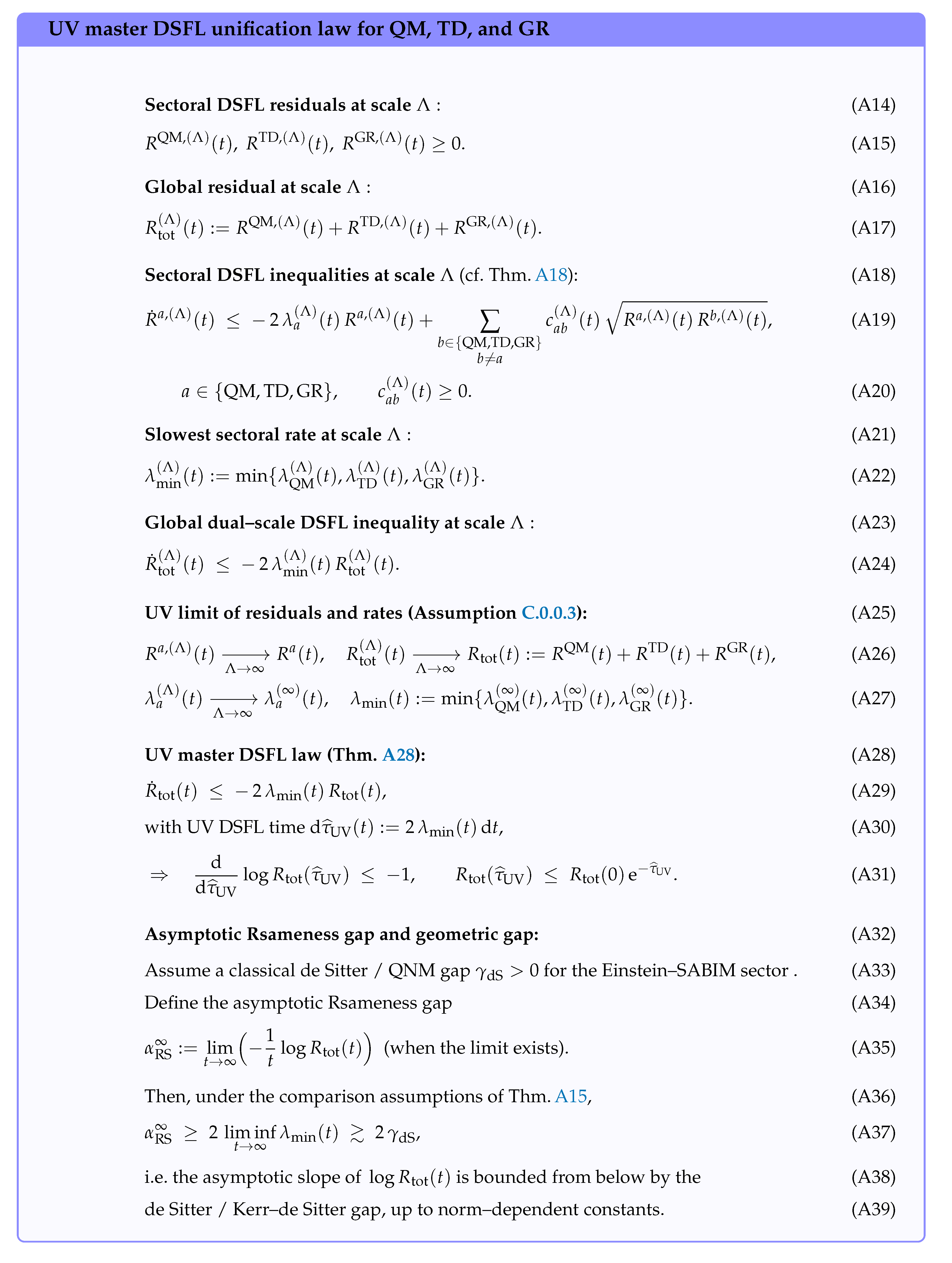
Appendix B. DSFL Unification Equation for QM, TD, GR and UV
In the DSFL framework the quantum, thermodynamic, and gravitational sectors are not evolved in isolation. Their sectoral residuals of sameness
are read in one common instrument geometry and add up to a single global residual
to which each sector contributes its own inner contraction rate , and .
At any finite UV cutoff , the sectoral Lyapunov inequalities established in sec:dual-scale-three,sec:uv-dsfl yield a global dual–scale inequality for the scale–resolved total residual , with the decay controlled by the slowest sectoral rate . Under the UV stability assumptions of ass:master-uv-stability, this structure passes to the limit and produces a single, scale–independent master DSFL inequality for the limiting global residual and a unified DSFL clock .
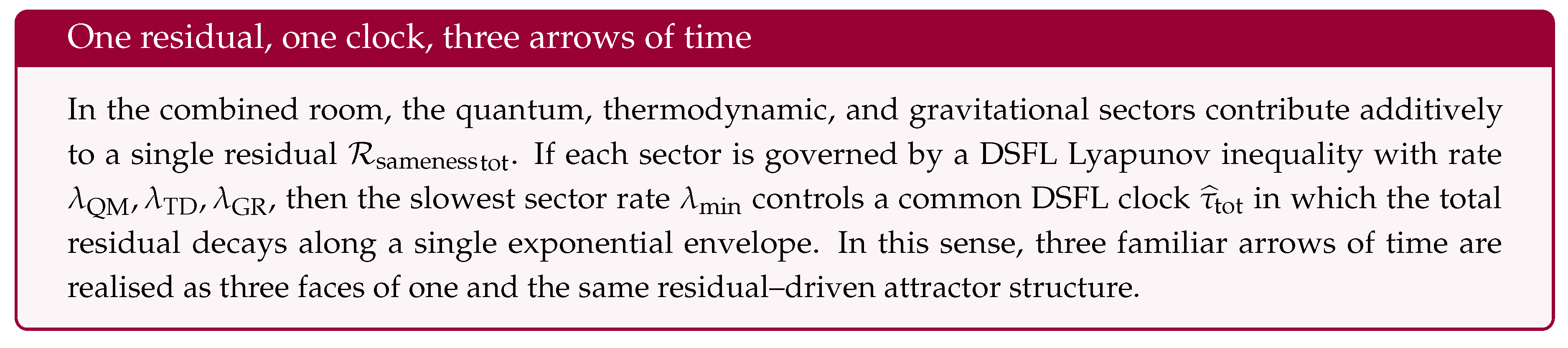
Phenomenologically, collapse and scrambling in QM, kinetic relaxation in TD, and curvature/ringdown in GR become three manifestations of one Lyapunov flow in a common residual geometry, with the effective arrow of time set by the slowest sector. For ease of reference, we collect the resulting three–sector (and optional QGR) UV master law in compact form below.
Remark A1.
In the three–sector DSFL room of this paper we take and label the sectors by , so that in (A93) becomes , with rates .
Appendix B.1. Explaining the DSFL Equations for QM, TD, GR and UV
For later use and for the reader’s convenience, we summarise here the structure of the DSFL equations that unify the quantum, thermodynamic and gravitational sectors, together with their UV completion. All precise statements and proofs are given in sec:dual-scale-three,sec:uv-dsfl and in the appendices; this subsection is a compact “reader’s guide” to the notation and content. The symbols , , , , , , and are summarised in Table A1.
Scale–resolved sectoral and global residuals.
For each UV cutoff and each sector we have a DSFL room
with sectoral defect and sectoral residual
Concretely, is the collapse/scrambling residual in the quantum DSFL room
Appendix C. Sector Rooms and UV Master Law
In the UV analysis we work with scale–resolved sector rooms for each cutoff . For each sector we write
for the DSFL residual in the corresponding sectoral room at scale . Concretely, is the collapse/scrambling residual in the quantum room (Section 3.1); is a –type kinetic residual in the thermodynamic room (Markov, Fokker–Planck, linearised Boltzmann), as in [6,7,19,72,73,74]; and is the squared norm of an Einstein–balance tensor in the gravitational room built from Einstein–SABIM PDE estimates.[22,75,76,77,78]
The global residual at scale is
and collects all mismatch across QM, TD and GR into a single scalar ledger. (An optional quantum–geometric sector , when used, is added in the same way.)
Sectoral DSFL inequalities and slowest rate.
On time scales where inner DSFL dynamics dominates, the sectoral residuals satisfy Lyapunov–type inequalities of the form
with and bounded couplings . Here is calibrated to collapse/scrambling rates and channel gaps in the quantum room (GKSL/quantum–information setting), comes from spectral gaps or hypocoercive constants for Markov and kinetic semigroups,[6,19,72,79] and is extracted from geometric energy decay and quasinormal–mode gaps in the Einstein–SABIM sector.[22,77,78] The couplings encode feed–down of residual between sectors (schematically ).
For each scale we define the slowest sectoral rate
Finite–cutoff global law.
Summing (A42) over a and absorbing the cross–terms with yields the global dual–scale inequality at scale (see Theorem A1 in Appendix J):
If then
Thus, at any fixed cutoff, the total mismatch across QM, TD and GR cannot decay more slowly than the rate set by the slowest sector.
UV limit and master DSFL law.
Assuming UV stability of residuals and rates we have
uniformly on compact time intervals, and hence
with limiting slowest rate
Passing to the limit in (A44) gives the UV master inequality (Theorem )
in the sense of distributions. Introducing the UV DSFL time
one obtains the one–slope UV law
This is the UV master DSFL unification equation: in DSFL time, the global residual decays at least with unit slope on a semilog plot, and the slowest sectoral rate sets the effective arrow of time. In the extended four–sector setting with and , the same construction goes through with included in the minima.
Gap comparison and emergent gravity.
In Kerr–de Sitter–type playgrounds the abstract rate can be tied directly to standard GR data. Let denote the de Sitter/Kerr–de Sitter gap, extracted either from quasinormal frequencies or from sharp local energy decay estimates,[22,77,78] and let be the geometric DSFL gap in the gravitational room. Defining the asymptotic Rsameness gap by
(when the limit exists), the gap–comparison theorem (Theorem A15 in the QG appendix) shows that, under the PDE/DSFL assumptions of Section C.0.0.4,
up to norm–dependent constants. Thus , and are three equivalent ways of reading off the late–time decay scale of the DSFL residual. Under additional microscopic assumptions,
Proposition A1
(Micro–gap to sector–gap). Let
be a microscopic DSFL room with microscopic defect and microscopic residual Assume that satisfies a DSFL Lyapunov inequality with microscopic gap , i.e.
Let
be a sectoral DSFL room (for example ), and let be a bounded linear coarse–graining map such that there exist constants with
Define the sectoral defect and residual by
Then itself obeys a DSFL Lyapunov inequality with a strictly positive sectoral gap:
where
In particular, if is an isometry between the instrument norms (i.e. ), then the sectoral gap coincides with the microscopic gap, .
In the UV–completed three–sector setting, the micro–gap to sector–gap result (Proposition A1) and the emergent–gravity theorem (Theorem A4) together show that the late–time tail of the global residual is governed by this same microscopic DSFL gap , and that in the UV limit gravity appears as the emergent slow DSFL sector whose decay rate controls the asymptotic Rsameness gap.
Theorem A4
(Emergent geometric sector). Let be the sectoral residuals of a three–sector DSFL system (QM, TD, GR), and let
be the global residual of sameness. Suppose that for almost every the sectoral residuals satisfy
for measurable rates and bounded couplings , and that the global residual obeys
Assume that there exist and such that for all ,
Then, for any initial data,
In particular, the global residual has a purely geometric tail,
where is any cluster point of as . Within the DSFL description, the gravitational sector is therefore the unique slow DSFL leg in the late–time regime: all surviving mismatch is carried by the geometric component of the single residual of sameness.
Appendix D. Calibrations
Appendix D.1. Gravitational Two–Loop Lyapunov Law
In the main text the GR calibration is described in terms of a defect built from the Einstein imbalance and a two–loop DSFL evolution (immediate loop + relay) acting on that defect (Section 3.3). The following theorem formalises the Lyapunov structure of such a two–loop evolution in an abstract Hilbert space; the Einstein imbalance case is obtained by choosing the underlying space and operators as in Definition 8. This isolates the purely operator–theoretic part of the GR DSFL law, independently of geometric details.
Theorem A5
(GR two–loop Lyapunov law). Let be a Hilbert space and let be a bounded, selfadjoint, strictly positive operator. Define the instrument inner product and norm by
Let be an absolutely continuous trajectory (the GR defect) solving the two–loop equation
where:
- (i)
- Immediate loop. For each , is bounded, selfadjoint in , and there exists a measurable function such that
- (ii)
-
Positive memory kernel. For each , the kernel is bounded and selfadjoint in and satisfiesMoreover, is weakly measurable and for each finite t, so the Volterra term in (A57) is well defined.
- (iii)
- Small remainder. There exists a measurable function such that for all and all ,
Define the gravitational DSFL residual
and the instantaneous decay rate
Then:
- (a)
- Lyapunov inequality.For almost every ,
- (b)
- Exponential envelope under a uniform gap.If there exists such that for all , then for all ,
- (c)
-
Intrinsic DSFL time.On any interval where , define the gravitational DSFL clock byThen along the trajectory one hasi.e. in intrinsic DSFL time the semilogarithmic plot has slope at most .
Proof.
We proceed in three steps.
Step 1: time derivative of the residual. By definition,
Since is absolutely continuous and is bounded, is absolutely continuous and differentiable almost everywhere, with
Substituting (A57) into (A67) gives
We estimate the three contributions separately.
Step 2: estimate of the immediate term. By selfadjointness of in , the first term in (A68) is real and equals
Using the coercivity assumption (A58) with , we obtain
Step 3: estimate of memory and remainder terms. Define the memory contribution
By Cauchy–Schwarz in and the positivity (A59) one has, for any fixed t,
so that
For the remainder, the bound (A60) gives
so
Step 4: Lyapunov inequality and DSFL rate. Combining (A67)–(A72) yields, for almost every ,
By definition (A62), this is exactly (A63), proving part (a).
Step 5: exponential envelope. Assume now that on . Then (A63) implies
The scalar Grönwall lemma (Theorem A7) gives
which is (A64). This proves part (b).
Step 6: intrinsic DSFL time and unit–slope envelope. On any interval where , define as in (A65). Whenever we can divide (A63) by to obtain
Using , we rewrite this as
which is (A66). If vanishes at some time, the inequality holds trivially by continuity. This proves part (c) and completes the proof. □
Remark A2
(Application to Einstein imbalance). In the gravitational calibration of Section 3.3, the defect is taken to be a perturbation of the Einstein imbalance in a suitable graph norm; encodes energy–type weights, arises from the linearised Einstein operator, and the memory kernel M collects retarded backreaction effects. Quasinormal–mode spectral gaps then provide natural candidates for lower bounds on , so that the DSFL rate is controlled by the least damped QNMs.[9,22,23,24] In this interpretation, is a DSFL residual for curvature–matter mismatch, and Theorem A5 is the abstract Lyapunov statement behind near–horizon ringdown envelopes in the Einstein–SABIM models discussed in Section C.0.0.4.
Appendix E. Spectral representation of DSFL residual dynamics
In this appendix we provide the functional–analytic derivations behind the spectral DSFL picture summarised in Section 5: the immediate operator , its eigenmodes, and the Lyapunov envelope for the residual.
Appendix E.1. DSFL room, defect, and residual
Throughout we work in a fixed DSFL room in the sense of Definition 1 in the main text. Given , the defect and residual are
For a time–dependent trajectory we write
Appendix E.2. Two–loop DSFL evolution and immediate damping
At the pDoF level, the abstract two–loop DSFL evolution used in the GR calibration has the form
where:
- is the immediate (time–local) part, bounded, selfadjoint and nonnegative in the instrument inner product ;
- is a remainder term, typically lower order and small in the sense of a form bound (see below).
Equation (A73) is the abstract DSFL version of “immediate damping + relay” used in the gravitational calibration.
Appendix E.3. Spectral decomposition of the immediate operator
For each fixed t let and be the corresponding instrument weight on . Introduce the similarity transform
Then is bounded, selfadjoint and nonnegative with respect to the underlying inner product . By the spectral theorem there exists an orthonormal basis and eigenvalues with
possibly accumulating at infinity in infinite dimension.[15,16]
Define the weighted defect
Expanding in the eigenbasis,
so the eigenvectors can be viewed as sameness modes for the immediate DSFL damping in the instrument norm.
Appendix E.4. Spectral DSFL differential inequality
We now derive a general differential inequality for in terms of the smallest eigenvalue of and a bound on the memory and remainder contributions.
Theorem A6
(Spectral DSFL differential inequality). Assume and satisfy the positivity and boundedness conditions above, and suppose the memory and remainder terms satisfy: there exists a measurable function such that for all ,
with and . Let
Set
Then, for almost every ,
Proof.
By definition,
so R is absolutely continuous and
From (A73) and ,
where, to lighten notation, the dependence on and is suppressed. Substituting yields
Using , the first term is
The last two terms are grouped as a correction and bounded in absolute value by via (A76). Hence
By definition of ,
so
with as claimed. □
Appendix E.5. Scalar DSFL lemma and DSFL clock
The previous theorem reduces the DSFL dynamics to a scalar differential inequality . For completeness we record the standard Grönwall lemma in this form.[15,16]
Theorem A7
(Scalar DSFL contraction lemma). Let be absolutely continuous and let be measurable. If
then, for all ,
In particular, if for all t, then for .
Proof.
Where we may write
Integrating from 0 to t gives
so
and the lower–bound case follows by . If at some time, the inequality holds trivially by continuity. □
Defining the DSFL clock by
the bound (A78) reads
In the ideal case (fixed and no remainder) one has , so the semilogarithmic plot of versus is an exact straight line of slope .
Appendix E.6. Finite–dimensional channel case
In finite dimension, DSFL admissibility and envelopes can be expressed purely in terms of a Gram operator.
Let be finite dimensional and strictly positive and selfadjoint. Equip with
A linear map induces
Theorem A8
(Spectral characterisation of DSFL admissibility). Let be bounded and define
where is the adjoint in the Hilbert–Schmidt inner product. Then:
- (a)
- .
- (b)
- Φ is DSFL–admissible (nonexpansive) iff , i.e. .
- (c)
- If for some , then for iterates and residuals one has
Proof.
For any ,
Writing , we get
Hence
proving (a). Nonexpansiveness is therefore equivalent to , i.e. , which is (b). For (c), if then and
which gives the geometric contraction. □
If we define the discrete DSFL clock by
then whenever ,
so the semilogarithmic plot of versus is an exact straight line of slope for any DSFL–admissible iteration. In this sense, in finite dimension DSFL admissibility is a purely spectral condition: the largest eigenvalue of fixes the slowest sameness mode, and is the discrete analogue of the continuous DSFL gap that appears in the continuous two–loop setting above.
Appendix F. Model–World Derivations
In this appendix we collect the elementary calculations underlying the toy examples in Section 4. The purpose is to verify explicitly that, in these simple finite–dimensional settings, the abstract DSFL residual reduces to familiar quadratic quantities and obeys the Lyapunov envelopes stated in the main text.
Appendix F.1. Amplitude–Damping Channel
We first give the algebraic details behind the amplitude–damping example used in Appendix F.1.
Proposition A2
(DSFL spectral envelope for the amplitude–damping channel). Let be the qubit amplitude–damping channel with parameter and fixed point , and work in the Hilbert–Schmidt DSFL calibration . For any initial state set
Then:
- (a)
- The Liouville superoperator of has spectrum , so the DSFL contraction factor on the traceless subspace in Hilbert–Schmidt norm is and the corresponding effective Lyapunov rate is .
- (b)
-
The residual sequence satisfies the spectral DSFL envelopewith equality (up to a constant prefactor) for generic initial states . Equivalently,so the semilogarithmic plot of versus k has asymptotic slope .
Proof.
Use the operator basis
for , and vectorise operators by stacking the coefficients in this ordered basis.
With Kraus operators
the channel is . A direct calculation yields
In the vectorised basis , the Liouville matrix therefore has the form
which is upper triangular with eigenvalues
This proves part (a).
Write any initial state as with traceless. Since , we have
so . In Liouville space, decomposes into eigenmodes of ; each component with eigenvalue decays as in Hilbert–Schmidt norm, hence contributes to .
On the traceless subspace the largest modulus eigenvalue is , so for generic (with a nonzero component in that eigenspace),
for some . In particular,
proving the envelope. Taking logarithms gives
so the asymptotic slope of versus k is . Setting yields and the stated form. □
Appendix F.2. Depolarising qubit
We now give the algebraic derivation underlying the depolarising example in Section 4.1. The proposition is stated in the main text as Proposition 2; here we only provide its proof.
Proof of Proposition 2.
We work in the quantum calibration with , , (Hilbert–Schmidt norm) and reference state . Any qubit state admits a Bloch representation
where are the Pauli matrices. The deviation from the reference state is
Using , we obtain
The depolarising channel
acts on Bloch vectors as
so
Therefore
which gives the single–step DSFL relation. Iterating k times yields , and rewriting identifies the constant rate and DSFL clock for which . □
Appendix F.3. Two–state Markov chain
Finally, we give the diagonalisation used in Section 4.2. The proposition is stated in the main text as Proposition A3; here we provide the proof.
Proposition A3
(Two–state TD DSFL envelope). Consider the two–state continuous–time Markov chain on with generator
Let
be the stationary distribution and choose the TD weight
so that . For a solution of the master equation
define the DSFL residual
Then
so is a strict Lyapunov functional, and in DSFL time one has .
Proof.
The eigenvalues of L are obtained from
so and we set . A stationary distribution satisfies and , which yields
as stated.
Let be the deviation from equilibrium. Since , we have for all t, so lies in the one–dimensional subspace orthogonal to the constant vector . In this subspace L acts as multiplication by : indeed,
Thus the solution of can be written as
By definition of , the DSFL residual is
Using ,
which is the claimed exponential law.
Finally, defining gives
so the semilogarithmic plot of versus DSFL time is a straight line of slope . □
Appendix G. DSFL Numerical Audits
This appendix is reserved for device–level and simulation–level DSFL audits (semilog Lyapunov fits, cone tests, band tests) for concrete models. In the present version we restrict ourselves to analytic model–world derivations (Appendix F); numerical audit plots and code will be reported separately when available.
Appendix H. DSFL Room, Admissibility, and Lyapunov Structure
In this appendix we collect the detailed proofs for the sector–neutral DSFL framework summarised in Section 2. We do not repeat the definitions; all labels refer to the main text.
Throughout, is a Hilbert space, closed subspaces, a bounded calibration map, and a strictly positive, selfadjoint instrument weight, as in Definition 1. The instrument inner product and norm are and .
Appendix H.1. Residual of sameness
Proof of Theorem 1.
Let and write . By Definition 1,
Since W is selfadjoint and strictly positive, for all and iff . Thus for all and iff , i.e. . The zero set of R is therefore exactly the calibration graph . □
Appendix H.2. Admissible Maps and DPI for R
Appendix H.3. Lyapunov Envelope and Intrinsic DSFL Time
Theorem A9
(Lyapunov inequality and DSFL clock). Let be a strongly continuous semigroup on with instrument weight , and suppose there is a measurable rate function such that for every initial defect the residual
is absolutely continuous and satisfies
Define the DSFL clock by
Then:
- (a)
- For all ,
- (b)
-
On any interval where , the map is strictly increasing, and along the trajectory one hasIn particular, in DSFL time the semilogarithmic plot has slope at most , with equality for ideal evolutions.
Proof.
Whenever we may divide (A79) by :
Integrating from 0 to t yields
so , and exponentiation gives (A81). If R vanishes at some time, the inequality holds trivially by continuity.
If in addition on an interval I, then for a.e. , so is strictly increasing and has an absolutely continuous inverse. On the set where and we then have
which gives the unit–slope bound in DSFL time. □
Appendix I. Frames, Principal Angles, and Budget Sharing
In this appendix we provide the proof of the principal–angle budget theorem used in Section 2 to quantify how two frames share the residual budget in a single DSFL norm.
Theorem A10
(Principal–angle budget across two frames). Let be a Hilbert space with norm , and let be closed subspaces with orthogonal projectors . Set
Then, for every ,
In particular, if (i.e. ), it is impossible to have and for the same nonzero vector e.
Proof.
Define a bounded linear map by
and equip with the product inner product
Then
By definition of the operator norm,
Since T is bounded,
where is the adjoint with respect to .
A direct computation shows
so
i.e.
Hence
For orthogonal projections it is a standard spectral fact (see e.g. [80] or [46]) that the nonzero spectrum of consists of eigenvalues , where range over the singular values of . In particular,
Thus
For general , write with . Then
as claimed.
For the incompatibility statement, suppose satisfies and . Then
By the inequality above,
so , i.e. . Since by definition, and . Thus if , no nonzero e can be fully captured by both frames; at least a fraction of the global budget lies outside one of them. □
Appendix J. Core DSFL Structural Lemmas
In this appendix we collect the minimal structural results that underlie the sector–neutral DSFL framework of Section 2 and the three–sector unification theorem of Section 3.4. Throughout we work in a fixed DSFL room in the sense of def:dsfl-room, and use the residual of sameness
Appendix J.1. Residual Positivity and Data–Processing
Theorem A11
(Positivity and zero set of the residual). In any DSFL room the residual satisfies
- (a)
- for all ;
- (b)
- if and only if .
Equivalently, the zero set of R is exactly the calibration graph
Proof.
For set . By definition,
where is the ambient inner product on . Since W is selfadjoint and strictly positive, one has for all and if and only if . Thus always, with equality if and only if , i.e. . This identifies the zero set with . □
Recall that a pair of bounded linear maps
is DSFL–admissible if (i) it preserves calibration, , and (ii) is nonexpansive in the instrument norm, for all (def:admissible).
Theorem A12
(Admissibility ⟺ DPI for R). Let be a DSFL room and let be bounded linear maps as above. Then the following are equivalent:
- (i)
- is DSFL–admissible;
- (ii)
- for all one has
Appendix J.2. Spectral Characterisation in Finite Dimension
In finite dimension it is convenient to encode nonexpansiveness in terms of a Gram operator.
Definition A2
(Gram operator and DSFL gap). Let be finite dimensional, strictly positive and selfadjoint on , and let be bounded. TheGram operatorof Φ in the instrument geometry is
where is the adjoint with respect to the ambient inner product on . The induced operator norm is
and the DSFL gap of Φ is
Lemma A1
(Spectral characterisation of nonexpansiveness). In the finite–dimensional setting of def:app-gram-gap one has
where denotes the largest eigenvalue. In particular, Φ is nonexpansive in if and only if , i.e. .
Proof.
For ,
Write , so and . Then
Taking the supremum over is equivalent to taking the supremum over , hence
This immediately yields the characterisation of nonexpansiveness. □
Appendix J.3. Scalar Lyapunov Lemma and DSFL Clock
The time–dependent DSFL Lyapunov statements in the main text reduce to a scalar Grönwall inequality once sectoral rates are known.
Theorem A13
(Scalar DSFL contraction lemma). Let be absolutely continuous and let be measurable. If
then for all ,
In particular, if on , then .
Proof.
Appendix J.4. Global Multi–Sector Lyapunov Inequality
Finally we record a general multi–sector version of the simple three–sector unification theorem in Section 3.4. It shows that, under mild coupling assumptions, the sum of sectoral residuals is controlled by the slowest sector rate.
Theorem A14
(Global multi–sector DSFL inequality). Let be absolutely continuous functions on satisfying, for almost every ,
where:
- are measurable rate functions;
- are measurable couplings with ;
-
there exists such that for all t,where .
Set . Then, for almost every ,
and hence
Proof.
In the three–sector QM+TD+GR toy of Section 3.4, one has , no positive couplings in the Lyapunov bounds (so ), and (A95) reduces exactly to the unification inequality used in the main text.
Theorem A15
(Gap comparison between de Sitter, DSFL and Rsameness). Let be the gravitational DSFL residual and the global residual of sameness for a three–sector DSFL system (QM, TD, GR), with UV master inequality
Assume:
- (a)
- (Einstein–SABIM gap).In a Kerr–de Sitter–type playground the Einstein–SABIM PDE estimates yield a de Sitter / quasinormal–mode gap , in the sense that local energy for linearised perturbations decays at least like in a suitable graph norm.
- (b)
-
(Gravitational DSFL gap).The GR sector is realised as a DSFL room with residual and satisfies a Lyapunov inequalityfor some geometric DSFL gap .
- (c)
-
(Global residual and asymptotic Rsameness gap).The global residual is finite for all , and the asymptotic Rsameness gapexists.
Then there exist positive constants , depending only on the DSFL norms and the Einstein–SABIM comparison constants, such that
and
In particular, the late–time decay scale of the global DSFL residual, the geometric DSFL gap, and the de Sitter / quasinormal–mode gap are equivalent up to fixed multiplicative constants.
Appendix K. Two–Qubit Bell Setup
In this section we fix a standard two–qubit Bell/CHSH configuration and its associated DSFL room. This setup underlies the nonlocality result in Appendix L and serves as a consistency check that the same single residual of sameness and the same instrument geometry used for collapse, scrambling and Einstein–SABIM residuals also reproduce standard quantum nonlocality (Tsirelson saturation) in a finite–dimensional test sector.[17,67,68,81]
Appendix K.1. Hilbert Space, Basis, and Pauli Operators
Let and be two qubit Hilbert spaces with computational bases
The standard Pauli operators are
and we write
for the corresponding local observables on .
The maximally entangled Bell state used in the CHSH test is
with density matrix In the DSFL language, is a particular pDoF configuration inside the finite–dimensional quantum room of Definition 6 (with Hilbert–Schmidt instrument norm), and Bell/CHSH experiments probe how this configuration responds to different DSFL–admissible measurement frames.
Appendix K.2. CHSH Observables and Bell Operator
We take the standard CHSH settings.[67,68,81]
These are selfadjoint unitaries with eigenvalues and can be realised as DSFL–admissible sharp instruments: their projectors form orthogonal frames in the same Hilbert–Schmidt geometry that underlies collapse as a nearest–point map in the canonical quantum DSFL room.[2,3,18,39,42]
The associated CHSH operator is
For a bipartite state , the CHSH value is
Classical local hidden–variable (LHV) models satisfy the CHSH bound , while quantum mechanics allows , with the maximal value attained, for example, by . This is the usual Tsirelson bound [68], which we reproduce here in a DSFL–calibrated setting.
Appendix K.3. Classical CHSH Bound
Theorem A16
(Classical CHSH bound). Consider an LHV model where each run is described by a hidden variable , with probability measure , and deterministic local outcomes
Define
Then .
Proof.
For fixed ,
Since , one of , equals and the other 0. Thus or , and . Therefore
□
Appendix K.4. Tsirelson Bound and Bell State Saturation
Theorem A17
(Tsirelson bound). Let and be selfadjoint operators with , on finite–dimensional . With
one has , and hence for all states ,
Proof.
Expanding,
Using and the usual algebra, one finds
where and similarly for B. Taking operator norms,
Each and is a unitary with eigenvalues , so and , . Thus and , as in the standard Tsirelson argument.[68] □
Proposition A4
(Bell state saturates Tsirelson). For as above and ,
Proof.
Using the standard identities
and the fact that cross terms such as have vanishing expectation on , one finds
Hence
□
This Bell/CHSH setup will be used in Appendix L to show that the DSFL residual framework, calibrated as in Definition 6, supports standard quantum nonlocality (Tsirelson saturation) while remaining norm–contractive and compatible with DSFL locality constraints.
Appendix L. DSFL Nonlocality in the Calibrated CHSH Sector
This appendix records a consistency check: the same quantum DSFL room used for collapse and residual dynamics also supports standard Bell nonlocality (Tsirelson saturation) while preserving DSFL admissibility and cone locality.[2,3,4,18,42]
Definition A3
(Two–qubit DSFL room for CHSH). Let , , and set
equipped with the Hilbert–Schmidt inner product . Define
Then the DSFL residual for a pair of states is
the two–qubit specialisation of the canonical quantum DSFL collapse room (cf. Section 3.1).[2,3,18]
In this calibration, DSFL admissibility for a channel is equivalent to , and Theorem 2 gives the single–residual DPI
so all CHSH dynamics we consider is norm–nonexpansive in the same sameness geometry.
Theorem A18
(DSFL nonlocality in the calibrated CHSH sector). In the two–qubit DSFL room of Definition A3:
- (a)
- (b)
- There exist DSFL–admissible data (the Bell state and local observables ) such that , saturating Tsirelson’s bound in the DSFL room.[68]
- (c)
Proof
(Proof sketch). (a) A local channel with corresponds to local pre– and post–processing of the marginal systems. Its action on CHSH statistics can be absorbed into an effective LHV model on the outcomes of and .[17,67,81] The classical CHSH bound then gives .
(b) The preparation of the Bell state followed by sharp measurements is DSFL–admissible: in the Hilbert–Schmidt metric, the Lüders projections onto eigenspaces of are orthogonal projectors (nearest–point maps) and hence DSFL–admissible sharp updates.[39,42] Standard CHSH analysis with these settings yields (Tsirelson saturation).[68]
(c) The CHSH protocol (local unitaries, projective measurements, and finite–dimensional ancillas) can be generated by a bounded local Hamiltonian on a finite tensor network or spin chain. For such local Hamiltonians, Lieb–Robinson–type bounds give cone–limited propagation in the Heisenberg picture,[11,12,13,14] and the cone–locality framework of Section 2.5 implies a bound of the form (13) in the Hilbert–Schmidt geometry. Hence the CHSH experiment in (b) is compatible with DSFL admissibility and microcausality. □
Together, (a)–(c) show that the calibrated DSFL two–qubit sector supports standard quantum nonlocality (Tsirelson–saturating CHSH violations) while maintaining DSFL contractivity and cone–limited propagation. In particular, the same single residual and instrument geometry that drive collapse, entropy production and Einstein–SABIM relaxation also support quantum Bell nonlocality, but no stronger–than–quantum (post–quantum) CHSH correlations, since the Tsirelson bound is enforced by the operator norm of C in the same Hilbert–space geometry.[17,68]
References
- Maldacena, J.; Shenker, S.H.; Stanford, D. A bound on chaos. Journal of High Energy Physics 2016, 2016, 106. [Google Scholar] [CrossRef]
- Nielsen, M.A.; Chuang, I.L. Quantum Computation and Quantum Information; Cambridge University Press, 2000.
- Watrous, J. The Theory of Quantum Information; Cambridge University Press, 2018.
- Wilde, M.M. Quantum Information Theory, 2nd ed.; Cambridge University Press: Cambridge, 2017. [Google Scholar]
- Horodecki, R.; Horodecki, P.; Horodecki, M.; Horodecki, K. Quantum Entanglement. Reviews of Modern Physics 2009, 81, 865–942. [Google Scholar] [CrossRef]
- Levin, D.A.; Peres, Y.; Wilmer, E.L. Markov Chains and Mixing Times; American Mathematical Society: Providence, RI, 2009; With contributions by James G. Propp and others. [Google Scholar]
- Villani, C. Hypocoercivity; Memoirs of the American Mathematical Society, American Mathematical Society: Providence, RI, 2009; Volume 202. [Google Scholar]
- Carlen, E.A.; Maas, J. Gradient flow and entropy inequalities for quantum Markov semigroups with detailed balance. Journal of Functional Analysis 2017, 273, 1810–1869. [Google Scholar] [CrossRef]
- Wald, R.M. General Relativity; University of Chicago Press: Chicago, 1984. [Google Scholar]
- Wald, R.M. Quantum Field Theory in Curved Spacetime and the Problem of Gravity; University of Chicago Press: Chicago, IL, 1994; Also published as Quantum Field Theory in Curved Spacetime and Black Hole Thermodynamics. [Google Scholar]
- Lieb, E.H.; Robinson, D.W. The finite group velocity of quantum spin systems. Communications in Mathematical Physics 1972, 28, 251–257. [Google Scholar] [CrossRef]
- Hastings, M.B. Lieb–Schultz–Mattis in higher dimensions. Physical Review B 2004, 69, 104431, [cond-mat/0305505]. [Google Scholar] [CrossRef]
- Bravyi, S.; Hastings, M.B.; Verstraete, F. Lieb–Robinson bounds and the generation of correlations and topological quantum order. Physical Review Letters 2006, 97, 050401, [quant-ph/0603121]. [Google Scholar] [CrossRef] [PubMed]
- Nachtergaele, B.; Sims, R. Lieb–Robinson bounds and the exponential clustering theorem. Communications in Mathematical Physics 2006, 265, 119–130, [math-ph/0506030]. [Google Scholar] [CrossRef]
- Kato, T. Perturbation Theory for Linear Operators, 2nd ed.; Springer: Berlin, 1976. [Google Scholar] [CrossRef]
- Reed, M.; Simon, B. Methods of Modern Mathematical Physics II: Fourier Analysis, Self-Adjointness; Academic Press: New York, 1975. [Google Scholar]
- Brunner, N.; Cavalcanti, D.; Pironio, S.; Scarani, V.; Wehner, S. Bell nonlocality. Rev. Mod. Phys. 2014, 86, 419–478. [Google Scholar] [CrossRef]
- Ohya, M.; Petz, D. Quantum Entropy and Its Use; Springer: Berlin, Heidelberg, 1993. [Google Scholar]
- Bakry, D.; Gentil, I.; Ledoux, M. Analysis and Geometry of Markov Diffusion Operators; Springer: Cham, 2013. [Google Scholar]
- Hawking, S.W. Particle creation by black holes. Communications in Mathematical Physics 1975, 43, 199–220. [Google Scholar] [CrossRef]
- Page, D.N. Information in black hole radiation. Physical Review Letters 1993, 71, 3743–3746, [hep-th/9306083]. [Google Scholar] [CrossRef]
- Berti, E.; Cardoso, V.; Starinets, A.O. Quasinormal modes of black holes and black branes. Classical and Quantum Gravity 2009, 26, 163001, [arXiv:gr-qc/0905.2975]. [Google Scholar] [CrossRef]
- Konoplya, R.A.; Zhidenko, A. Quasinormal modes of black holes: From astrophysics to string theory. Reviews of Modern Physics 2011, arXiv:gr-qc/1102.4014]83, 793–836. [Google Scholar] [CrossRef]
- Dafermos, M.; Holzegel, G.; Rodnianski, I. Title of the Article. Journal Name Year, Volume, Pages. Add full details here.
- Maldacena, J.M. The Large N Limit of Superconformal Field Theories and Supergravity. Advances in Theoretical and Mathematical Physics 1998, 2, 231–252, [hep-th/9711200]. [Google Scholar] [CrossRef]
- Ryu, S.; Takayanagi, T. Holographic Derivation of Entanglement Entropy from AdS/CFT. Physical Review Letters 2006, 96, 181602. [Google Scholar] [CrossRef]
- Raamsdonk, M.V. Building up spacetime with quantum entanglement. General Relativity and Gravitation 2010, 42, 2323–2329. [Google Scholar] [CrossRef]
- Hayden, P.; Preskill, J. Black holes as mirrors: quantum information in random subsystems. Journal of High Energy Physics 2007, 2007, 120. [Google Scholar] [CrossRef]
- Sekino, Y.; Susskind, L. Fast Scramblers. Journal of High Energy Physics 2008, 2008, 065. [Google Scholar] [CrossRef]
- Lindblad, G. Completely Positive Maps and Entropy Inequalities. Communications in Mathematical Physics 1975, 40, 147–151. [Google Scholar] [CrossRef]
- Lindblad, G. On the generators of quantum dynamical semigroups. Communications in Mathematical Physics 1976, 48, 119–130. [Google Scholar] [CrossRef]
- Uhlmann, A. Relative Entropy and the Wigner–Yanase–Dyson Skew Information. Communications in Mathematical Physics 1977, 54, 21–32. [Google Scholar] [CrossRef]
- Petz, D. Monotonicity of quantum relative entropy revisited. Quantum Information & Computation 2003, 3, 134–140, [arXiv:quant-ph/quant-ph/0209053]. [Google Scholar]
- Bhatia, R. Matrix Analysis; Vol. 169, Graduate Texts in Mathematics, Springer: New York, 1997. [CrossRef]
- Gorini, V.; Kossakowski, A.; Sudarshan, E.C.G. Completely positive dynamical semigroups of N-level systems. Journal of Mathematical Physics 1976, 17, 821–825. [Google Scholar] [CrossRef]
- Lindblad, G. On the generators of quantum dynamical semigroups. Communications in Mathematical Physics 1976, 48, 119–130. [Google Scholar] [CrossRef]
- Hollands, S.; Wald, R.M. Quantum fields in curved spacetime. Reviews of Modern Physics 2008, 80, 1083–1159. [Google Scholar] [CrossRef]
- Spohn, H. Entropy production for quantum dynamical semigroups. Journal of Mathematical Physics 1978, 19, 1227–1230. [Google Scholar] [CrossRef]
- Lueders, G. Title Placeholder. Journal Placeholder 1951, 1, 1–10. [Google Scholar]
- Gleason, A.M. Measures on the Closed Subspaces of a Hilbert Space. Journal of Mathematics and Mechanics 1957, 6, 885–893. [Google Scholar] [CrossRef]
- Busch, P.; Lahti, P.; Werner, R.F. Measurement Uncertainty Relations. Journal of Mathematical Physics 2014, 55, 042111. [Google Scholar] [CrossRef]
- Busch, P.; Lahti, P.; Werner, R.F. Colloquium: Quantum Root-Mean-Square Error and Measurement Uncertainty Relations. Reviews of Modern Physics 2014, 86, 1261–1281. [Google Scholar] [CrossRef]
- Ringström, H. The Cauchy Problem in General Relativity; European Mathematical Society: Zürich, 2009. [Google Scholar]
- Jordan, C. Essai sur la géométrie à n dimensions. Bulletin de la Société Mathématique de France 1875. Classic introduction of principal (canonical) angles; bibliographic details vary by edition.
- Friedrichs, K. On Certain Inequalities and Characteristic Angles. Annals of Mathematics 1937. Hilbert-space formulation of the angle between subspaces (Friedrichs angle).
- Davis, C.; Kahan, W.M. The Rotation of Eigenvectors by a Perturbation. SIAM Journal on Numerical Analysis 1970, 7, 1–46. [Google Scholar] [CrossRef]
- von Neumann, J. Mathematische Grundlagen der Quantenmechanik; Springer: Berlin, 1932. English translation by R. T. Beyer: Mathematical Foundations of Quantum Mechanics, Princeton University Press, 1955.
- Halperin, I. The Product of Projection Operators. Acta Scientiarum Mathematicarum (Szeged) 1962, 23, 96–99. [Google Scholar]
- Deutsch, F. The method of alternating orthogonal projections. Transactions of the American Mathematical Society 1965, 118, 272–276. [Google Scholar]
- Bauschke, H.H.; Borwein, J.M. On Projection Algorithms for Solving Convex Feasibility Problems. SIAM Review 1996, 38, 367–426. [Google Scholar] [CrossRef]
- Deutsch, F.; Hundal, H. The Rate of Convergence for the Method of Alternating Projections. Journal of Approximation Theory 2006, 141, 63–77. [Google Scholar]
- Heisenberg, W. Über den anschaulichen Inhalt der quantentheoretischen Kinematik und Mechanik. Zeitschrift für Physik 1927, 43, 172–198. [Google Scholar] [CrossRef]
- Robertson, H.P. The Uncertainty Principle. Physical Review 1929, 34, 163–164. [Google Scholar] [CrossRef]
- Schrödinger, E. Zum Heisenbergschen Unschärfeprinzip. Sitzungsberichte der Preussischen Akademie der Wissenschaften, Physikalisch-mathematische Klasse 1930, pp. 296–303.
- Hirschman, I. I., J. A Note on Entropy. American Journal of Mathematics 1957, 79, 152–156. [Google Scholar] [CrossRef]
- Beckner, W. Inequalities in Fourier Analysis. Annals of Mathematics 1975, 102, 159–182. [Google Scholar] [CrossRef]
- Białynicki-Birula, I.; Mycielski, J. Uncertainty Relations for Information Entropy in Wave Mechanics. Communications in Mathematical Physics 1975, 44, 129–132. [Google Scholar] [CrossRef]
- Maassen, H.; Uffink, J.B.M. Generalized Entropic Uncertainty Relations. Physical Review Letters 1988, 60, 1103–1106. [Google Scholar] [CrossRef]
- Ozawa, M. Universally valid reformulation of the Heisenberg uncertainty principle on noise and disturbance in measurement. Physical Review A 2003, 67, 042105. [Google Scholar] [CrossRef]
- Naimark, M.A. Spectral functions of a symmetric operator. Izvestiya Akademii Nauk SSSR. Seriya Matematicheskaya 1940, 4, 277–318. [in Russian]; English transl. Amer. Math. Soc. Transl. (2) 16 (1960), 103–239.
- Stinespring, W.F. Positive functions on C*-algebras. Proceedings of the American Mathematical Society 1955, 6, 211–216. [Google Scholar] [CrossRef]
- Haag, R. Local Quantum Physics: Fields, Particles, Algebras, 2nd ed.; Springer: Berlin, 1996. [Google Scholar] [CrossRef]
- Bisognano, J.J.; Wichmann, E.H. On the Duality Condition for a Hermitian Scalar Field. Journal of Mathematical Physics 1975, 16, 985–1007. [Google Scholar] [CrossRef]
- Bratteli, O.; Robinson, D.W. Operator Algebras and Quantum Statistical Mechanics I, 2nd ed.; Springer: Berlin, 1987. [Google Scholar] [CrossRef]
- Takesaki, M. Theory of Operator Algebras II; Vol. 125, Encyclopaedia of Mathematical Sciences, Springer: Berlin, Heidelberg, 2003. [CrossRef]
- Kochen, S.; Specker, E.P. The Problem of Hidden Variables in Quantum Mechanics. Journal of Mathematics and Mechanics 1967, 17, 59–87. [Google Scholar] [CrossRef]
- Bell, J. On the Einstein Podolsky Rosen paradox. Physics 1964, 1, 195–200. [Google Scholar] [CrossRef]
- Tsirelson, B.S. Quantum generalizations of Bell’s inequality. Letters in Mathematical Physics 1980, 4, 93–100. [Google Scholar] [CrossRef]
- von Neumann, J. Mathematische Grundlagen der Quantenmechanik; Springer: Berlin, 1932. [Google Scholar]
- Stone, M.H. Linear transformations in Hilbert space. III. Operational methods and group theory. Proceedings of the National Academy of Sciences of the United States of America 1930, 16, 172–175. [Google Scholar] [CrossRef]
- von Neumann, J. Die Eindeutigkeit der Schrödingerschen Operatoren. Mathematische Annalen 1931, 104, 570–578. [Google Scholar] [CrossRef]
- Bakry, D.; Émery, M. Diffusions hypercontractives. In Séminaire de probabilités XIX 1983/84; Azéma, J., Meyer, P.A., Yor, M., Eds.; Springer: Berlin, 1985; Volume 1123, Lecture Notes in Mathematics; pp. 177–206. [Google Scholar] [CrossRef]
- Cercignani, C.; Illner, R.; Pulvirenti, M. The Mathematical Theory of Dilute Gases; Vol. 106, Applied Mathematical Sciences, Springer: New York, 1994. [CrossRef]
- Mouhot, C.; Neumann, L. Quantitative perturbative study of convergence to equilibrium for collisional kinetic models in the torus. Nonlinearity 2006, 19, 969–998. [Google Scholar] [CrossRef]
- Christodoulou, D.; Klainerman, S. The Global Nonlinear Stability of the Minkowski Space; Princeton Mathematical Series; Princeton University Press: Princeton, NJ, 1993; Volume 41. [Google Scholar]
- Dafermos, M.; Rodnianski, I. Decay for solutions of the wave equation on Kerr exterior spacetimes I: The cases |a|≪M or axisymmetry. arXiv preprint 2010, arXiv:1010.5132. [Google Scholar]
- Dafermos, M.; Holzegel, G.; Rodnianski, I. The Linear Stability of the Schwarzschild Solution to Gravitational Perturbations. Acta Mathematica 2019, 222, 1–214. [Google Scholar] [CrossRef]
- Hintz, P.; Vasy, A. The Global Non-Linear Stability of the Kerr–de Sitter Family of Black Holes. Acta Mathematica 2018, 220, 1–206. [Google Scholar] [CrossRef]
- Villani, C. Hypocoercivity; Number 950 in Memoirs of the American Mathematical Society, American Mathematical Society: Providence, RI, 2009. [Google Scholar]
- Björck, Å.; Golub, G.H. Numerical methods for computing angles between linear subspaces. Mathematics of Computation 1973, 27, 579–594. [Google Scholar] [CrossRef]
- Clauser, J.F.; Horne, M.A.; Shimony, A.; Holt, R.A. Proposed Experiment to Test Local Hidden-Variable Theories. Physical Review Letters 1969, 23, 880–884. [Google Scholar] [CrossRef]
Disclaimer/Publisher’s Note: The statements, opinions and data contained in all publications are solely those of the individual author(s) and contributor(s) and not of MDPI and/or the editor(s). MDPI and/or the editor(s) disclaim responsibility for any injury to people or property resulting from any ideas, methods, instructions or products referred to in the content. |
© 2025 by the authors. Licensee MDPI, Basel, Switzerland. This article is an open access article distributed under the terms and conditions of the Creative Commons Attribution (CC BY) license (http://creativecommons.org/licenses/by/4.0/).
Copyright: This open access article is published under a Creative Commons CC BY 4.0 license, which permit the free download, distribution, and reuse, provided that the author and preprint are cited in any reuse.


