From Marginal Entropy to Calibrated Sameness: Reframing the Black-Hole Information Paradox with DSFL

1. Introduction

Black–hole evaporation brings three venerable principles into sharp relief: global quantum evolution is (effectively) unitary; semiclassical effective field theory (EFT) is accurate at low curvature outside the horizon; and infalling observers see “no drama” at the horizon [1,2,3,4]. Hawking’s calculation, however, makes the exterior flux locally thermal, and when one tracks the von Neumann entropy of the radiation marginal it appears to grow monotonically—in tension with the unitary Page curve unless one sacrifices semiclassics or horizon regularity. Recent island/replica computations recover a unitary Page curve within semiclassical gravity by reassigning entanglement wedges [5,6], but they still leave open a clean, channel–level statement of what semiclassics guarantees and what must be relegated to correlations.

1.1. A Single Yardstick

This paper proposes and develops a minimal, sector–neutral yardstick for “information” that lives where both the statistical description and the physical response can be compared: a single Hilbert geometry $(\mathcal{H},\langle ·,·\rangle )$. We embed a statistical blueprint channel $\mathsf{S}$ (sDoF) and a physical response channel $\mathsf{P}\subset \mathcal{H}$ (pDoF), linked by interchangeability (calibration) maps

$$\mathcal{I}:\mathsf{S}\to \mathsf{P},J^{(+)}:\mathsf{P}\to \mathsf{S},\mathcal{I}{J}^{(+)}={\mathrm{id}}_{\mathsf{P}},J^{(+)}\mathcal{I}=P_{\mathsf{S}}.$$

The only observable we track is the calibrated residual of sameness

$$R(s,p):=\parallel p-\mathcal{I}s{\parallel }_{\mathcal{H}}^2,$$

(1)

which vanishes iff the device output pis the calibrated image $\mathcal{I}s$ of the blueprint. In this language, “information flow’’ is simply the contraction of R.

1.2. Two Structural Principles

(i) Admissibility ⇒ data–processing. A physical update $(\tilde{\mathsf{\Phi }},\mathsf{\Phi })$ is admissible if it intertwines the calibration and is nonexpansive in $\mathcal{H}$: $\mathsf{\Phi }\mathcal{I}=\mathcal{I}\tilde{\mathsf{\Phi }},{\parallel \mathsf{\Phi }\parallel }_{\mathcal{H}\to \mathcal{H}}\le 1.$ Then

$$R(\tilde{\mathsf{\Phi }}s,\mathsf{\Phi }p)=\parallel \mathsf{\Phi }\left(p-\mathcal{I}s\right){\parallel }_{\mathcal{H}}^2\le {\parallel p-\mathcal{I}s\parallel }_{\mathcal{H}}^2=R(s,p),$$

(2)

a one–line Hilbertian data–processing inequality (DPI) [7,8]. In particular, no admissible coarse–graining, counting, or channel concatenation can increase the calibrated misfit.

(ii) Dual–scale feedback ⇒ exterior envelope & causal ceiling. When dynamics are present, the calibrated misfit $e:=p-\mathcal{I}s$ evolves by a universal two–loop law:

$$\dot{e}\left(t\right)=-K_{\ell }e\left(t\right)-{\int }_0^{t}M(t-\tau )e\left(\tau \right)d\tau +r\left(t\right),$$

with a fast local dissipative loop $K_{\ell }⪰0$ and a slow nonlocal causal relay $M\in L^1\left([0,\infty )\right)$ (the memory kernel) [9]. Horizons throttle the slow loop: the retarded kernel has null/timelike support and cannot relay calibrated content across the event horizon [1,2]. The exterior then closes to ${\dot{e}}_U=-K_{\ell }{e}_U+r_U,$ so the exterior residual $R_{\mathrm{out}}\left(t\right)={\parallel e_U\left(t\right)\parallel }_{\mathcal{H}}^2$ obeys a Lyapunov envelope with a ringdown slope set by the least–damped mode (red–shift/QNM) [10,11].

1.3. Hawking as an Admissible Channel

A single “Hawking tick’’—pair creation near the horizon followed by tracing the interior partner—is a completely positive, unital step in the Heisenberg picture (Stinespring/Kraus), hence nonexpansive in the natural $L^2$ geometry [7,12]. Modeled as $({\tilde{\mathsf{\Phi }}}_{\mathrm{Hawk}},{\mathsf{\Phi }}_{\mathrm{Hawk}})$, it satisfies (2) stepwise: $R({\tilde{\mathsf{\Phi }}}_{\mathrm{Hawk}}s,{\mathsf{\Phi }}_{\mathrm{Hawk}}p)\le R(s,p).$ Local KMS thermality of exterior marginals is compatible with this DPI; microstate dependence can reside in correlations (early/late radiation, or island wedges) without forcing any increase of exterior R [3,4,5,6].

1.4. What This Buys

The usual trilemma (unitarity, semiclassical exterior EFT, no drama) is a tension about the wrong observable: marginal entropy of subsystems. In contrast, semiclassics proves monotone contraction of a single quadratic functional R (globally and outside the horizon), and, with red–shift control, an explicit exterior decay envelope. Purification is then necessarily a statement about correlations, not about local residuals. In this paper we:

• formalize the DSFL kinematics (interchangeability, R, admissibility) and prove the global/exterior DPIs;
• derive a causal “no–relay’’ barrier at the horizon and a Lyapunov (ringdown) envelope for $R_{\mathrm{out}}$;
• model Hawking ticks as admissible channels, reconciling local thermality with stepwise contraction;
• show how a one–budget convention (probability share $w{s}_0$) encodes “no duplication of description’’ while allowing redistribution and long–range correlations; and
• spell out falsifiable diagnostics (projection+DPI checks, semi–log ringdown slopes, relay toggles, and radiation correlation structure) that do not depend on any microscopic island model.

1.5. Roadmap

Section 2 gives a two–page primer on the comparison geometry, interchangeability, the residual $\mathcal{R}$, and admissibility. sec:bh-info-paradox then states the trilemma and sets the DSFL kinematics, proving a global/exterior Hilbertian DPI and deriving the dual–scale (fast/slow) feedback law with a causal ceiling at the horizon, which yields an exterior Lyapunov (ringdown) envelope from red–shift/QNM coercivity. Next, in Hawking channel as an admissible map we model each “tick’’ as a Stinespring/Kraus CP–unital step and show stepwise $L^2$-nonexpansiveness (with supporting operator–algebra citations), reconcile local KMS thermality with monotone exterior R, and connect to Page/island purification via correlations. The subsection Form of the paradox in DSFL variables restates what is actually constrained (the calibrated misfit R), followed by Resolution template giving stand-alone statements with proofs/sketches (no-inflation, causal throttling, exterior envelope, Hawking admissibility, global DPI). We then provide What can be tested (Section 7.3)—a falsifiability/diagnostics suite—and a geometric add-on (subspace–angle contraction) for calibration quality and per-step guarantees. Appendices include notation and a Generic Two–Channel Application Template for porting the scheme to other sectors. Throughout, the mathematics is deliberately elementary (orthogonal projections, nonexpansive maps in $\mathcal{H}$, Stinespring/Kraus), while the physics enters through causality and established exterior decay mechanisms.

2. DSFL in Two Pages (Self-Contained Primer for New Readers)

Discussions of “information loss” or “purification” often compare quantities that live in different mathematical spaces (fields, states, coarse-grained observables). To reason cleanly about what can or cannot increase under physically allowed operations, we place both sides of the description—statistics and physics— into one Hilbert geometry and measure a single, objective gap. The DSFL claim is deliberately modest: once statistics and physics are co-located in a common geometry, the one observable that semiclassics can provably control is a calibrated $L^2$-residual. Everything else (e.g. purification) is delegated to correlations rather than to local marginals.

2.1. Common Comparison Geometry.

Fix a (real or complex) Hilbert space $(\mathcal{H},\langle ·,·\rangle )$ with norm $\parallel x\parallel :=\sqrt{\langle x,x\rangle }$. We embed:

- a statistical blueprint channel $\mathsf{S}$ (what the model “asks” for), and - a physical response channel $\mathsf{P}\subset \mathcal{H}$ (what the system “does”)

in the same $\mathcal{H}$. This co-location makes comparisons well-typed, Euclidean, and orthogonalizable.

2.2. Interchangeability (Calibration) Maps.

A calibration pair

$$\mathcal{I}:\mathsf{S}\to \mathsf{P},J^{(+)}:\mathsf{P}\to \mathsf{S}$$

is required to satisfy

$$\mathcal{I}{J}^{(+)}={\mathrm{id}}_{\mathsf{P}},J^{(+)}\mathcal{I}=P_{\mathsf{S}},$$

(3)

where $P_{\mathsf{S}}$ is the orthogonal projector onto the blueprint subspace $\mathsf{S}\subset \mathcal{H}$. Equation (3) encodes two-way coherence: pushing a physical response to the blueprint and back is the identity on the physical side; pulling a blueprint to the physical side and back projects to the canonical blueprint subspace. Intuitively, $(\mathcal{I},J^{(+)})$ is the calibrated meter that says when “model” and “device” are literally the same object in $\mathcal{H}$.

2.3. Residual of Sameness.

With $(s,p)\in \mathsf{S}\times \mathsf{P}$ we track a single observable—the calibrated misfit

$$\mathcal{R}(s,p):=\parallel p-\mathcal{I}s{\parallel }_{\mathcal{H}}^2\ge 0,\mathcal{R}(s,p)=0⟺p=\mathcal{I}s\left(\mathrm{perfect}\mathrm{match}\right).$$

(4)

$\mathcal{R}$ is the “thermometer” for sameness: it vanishes iff the physical response is exactly the calibrated image of the blueprint. Because $\mathcal{R}$ is purely metric in $\mathcal{H}$, it is invariant under any isometry $U:\mathcal{H}\to \mathcal{H}$ with $U\left(\mathrm{Im}\mathcal{I}\right)=\mathrm{Im}\mathcal{I}$ (change of basis, polarization, or coordinates that preserve the calibrated image).

2.4. Admissible (Physically Allowed) Updates.

An update $(\tilde{\mathsf{\Phi }},\mathsf{\Phi })$—think “model step” on $\mathsf{S}$ and “physical step” on $\mathsf{P}$—is admissible if it satisfies

$$\mathsf{\Phi }\mathcal{I}=\mathcal{I}\tilde{\mathsf{\Phi }}{(\mathrm{intertwining}\mathrm{of}\mathrm{calibration})\mathrm{and}\parallel \mathsf{\Phi }\parallel }_{\mathcal{H}\to \mathcal{H}}\le 1(\mathrm{nonexpansive}/\mathrm{contractive}\mathrm{in}\mathcal{H}).$$

(5)

The first identity says “do the model step and then calibrate” equals “calibrate and then do the physical step.” The second says the physical step cannot amplify distances in the comparison geometry. Both properties are stable under composition, so sequences and flows of admissible maps remain admissible.

2.5. Data–Processing Inequality (DPI) in One Line.

From (5) and (4):

$$\mathcal{R}(\tilde{\mathsf{\Phi }}s,\mathsf{\Phi }p)=\parallel \mathsf{\Phi }(p-\mathcal{I}s){\parallel }_{\mathcal{H}}^2\le {\parallel p-\mathcal{I}s\parallel }_{\mathcal{H}}^2=\mathcal{R}(s,p).$$

(6)

Thus no admissible evolution can inflate the calibrated residual. This is the core monotonicity we use throughout: it supplies an intrinsic “arrow” independent of coordinates, coarse-graining, or the parametrization of time. In particular, DPI is “clock-neutral”: it holds identically for any ordering of admissible steps and any strictly increasing reparametrization of the evolution parameter.

2.6. One-Budget Convention (No Duplication of Description).

To make “no cloning of description” concrete, we represent the statistical content as a reweighting of a fixed prototype:

$$s(·,t)=w(·,t)s_0,w\ge 0,\int wd\mu =1.$$

(7)

Admissible updates may redistribute the share w (move blueprint weight around) but cannot create new statistical degrees of freedom. This “one stock of sDoF” rule prevents paradoxes driven by hidden double-counting: every apparent “split” in presentation is a partition of the same budget, not the birth of an additional prototype.

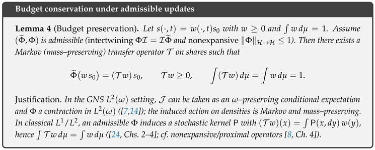
Lemma 1

(Budget preservation as a Markov pushforward). Assume the one–budget ansatz $s(·,t)=w(·,t)s_0$ with $w\ge 0$, $\int wd\mu =1$. If $(\tilde{\mathsf{\Phi }},\mathsf{\Phi })$ is admissible and $\tilde{\mathsf{\Phi }}$ acts locally on w through a linear positive operator $\mathcal{T}$ (i.e. $\tilde{\mathsf{\Phi }}\left(w{s}_0\right)=\left(\mathcal{T}w\right)s_0$), then $\mathcal{T}$ is Markov:

$$\mathcal{T}w\ge 0,\int \left(\mathcal{T}w\right)d\mu =\int wd\mu =1.$$

Proof. 

Positivity follows from positivity of $\tilde{\mathsf{\Phi }}$. For mass, test against the constant functional induced by $J^{(+)}\mathcal{I}=P_{\mathsf{S}}$:

$$\int \left(\mathcal{T}w\right)d\mu =\langle \mathbf{1},\mathcal{T}w\rangle =\langle J^{(+)}\mathcal{I}\mathbf{1},\mathcal{T}w\rangle =\langle J^{(+)}\left(\mathsf{\Phi }\mathcal{I}\mathbf{1}\right),w\rangle =\langle \mathbf{1},w\rangle =\int wd\mu ,$$

using intertwining $\mathsf{\Phi }\mathcal{I}=\mathcal{I}\tilde{\mathsf{\Phi }}$ and $\mathcal{I}\mathbf{1}=\mathbf{1}$ after normalization. □

Corollary 1

(No duplication of calibrated content). Under Lemma 1 and Prop. 2, no admissible $(\tilde{\mathsf{\Phi }},\mathsf{\Phi })$ can map one input budget w to two independent identical budgets $w_1,w_2$ with $\int w_1=\int w_2=1$ while preserving the same calibrated content on both outputs. In particular, perfect broadcasting of noncommuting presentations is impossible unless they share a common abelian pointer subalgebra.

Proof. 

Two independent identical full budgets would violate $\int wd\mu =1$ (mass creation) or force an isometric duplication of the residual direction, contradicting DPI nonexpansiveness. Broadcasting of noncommuting data would likewise require residual nonincrease for two incompatible marginals simultaneously; this is precluded unless they commute. □

2.7. Dual–Scale Feedback (Immediate Local Loop, Slow Nonlocal Relay).

For dynamics we use a Volterra-type two-loop law for the calibrated mismatch $e:=p-\mathcal{I}s$:

$$\dot{e}\left(t\right)=-K_{\mathrm{imm}}e\left(t\right)-{\int }_0^{t}M(t-\tau )e\left(\tau \right)d\tau +r\left(t\right),$$

(8)

where the immediate loop $-K_{\mathrm{imm}}e$ acts locally (modewise or pointwise) in $\mathcal{H}$ and $M(·)⪰0$ captures slow, causal nonlocal relay; r is a small admissible remainder. If $K_{\mathrm{imm}}$ is positive (and, when needed, coercive on the exterior), then the energy identity

$${\displaystyle \frac{d}{dt}}{\parallel e\left(t\right)\parallel }_{\mathcal{H}}^2=-2\langle K_{\mathrm{imm}}e,e\rangle +2\langle r,e\rangle$$

gives a Lyapunov envelope once $\langle K_{\mathrm{imm}}x,x\rangle \ge \kappa {\parallel x\parallel }^2$ and $\left|\langle r,e\rangle \right|\le {\epsilon \parallel e\parallel }^2$:

$$\dot{\mathcal{R}}\left(t\right)\le -2(\kappa -\epsilon )\mathcal{R}\left(t\right)\Rightarrow \mathcal{R}\left(t\right)\le e^{-2(\kappa -\epsilon )(t-t_0)}\mathcal{R}\left(t_0\right).$$

The slow relay is retarded and, under causal support restrictions, cannot instantaneously spread calibrated content across forbidden domains (e.g. across a horizon), which is the DSFL “no-relay” statement.

2.7.1. Clock-Neutrality and Intrinsic DSFL-Time.

All DSFL conclusions above are invariant under any strictly increasing reparametrization of the evolution parameter: if $\theta =\theta \left(t\right)$, then ${\displaystyle \frac{dR}{d\theta }}={\displaystyle \frac{dR}{dt}}{\displaystyle \frac{dt}{d\theta }}$ preserves the sign and thus the monotonicity. A convenient intrinsic clock is

$$d\widehat{\tau }:=2\kappa \left(t\right)dt\Rightarrow {\displaystyle \frac{dR}{d\widehat{\tau }}}\le -R,$$

so $R\left(\widehat{\tau }\right)\le e^{-(\widehat{\tau }-{\widehat{\tau }}_0)}R\left({\widehat{\tau }}_0\right)$ has unit slope in semi–log scale, independent of the original time parameter. This fixes a canonical “DSFL-time” for comparing decay rates across settings.

What this buys us. With (3)–(8) in place, everything we claim in the conclusions—no inflation of exterior residuals (DPI), ringdown Lyapunov envelopes driven by the immediate loop, causal “no-relay” across horizons for the slow loop, and the compatibility of local thermality with global purification— follows from standard Hilbert-space geometry (orthogonal projections, contractive maps) and causal support of the memory term. No new entropy axioms are needed; the single observable $\mathcal{R}$ serves as the conserved “ledger of sameness.”

2.8. What in DSFL Resolves the Paradox (Concise, Technical Summary)

2.8.1. Core Idea.

In DSFL, the “resolution” is not a new microscopic ingredient but a reformulation that turns the paradox into theorems about the right observable and the right causality constraints. The key moves are:

• Replace ‘‘information’’ by the calibrated residual of sameness

  $$R:={\parallel p-\mathcal{I}s\parallel }^2.$$

  What this does: Puts the statistical blueprint s (sDoF) and the physical response p (pDoF) in the same Hilbert geometry and measures a single, objective mismatch. Why that helps: Semiclassical evolution can be proven to contract R. EFT controls R—not a marginal von Neumann entropy. The traditional contradiction arose from constraining the wrong quantity.
• Admissibility ⇒ a one-line DPI for R (global and exterior).
  Statement: For any physically allowed step $(\tilde{\mathsf{\Phi }},\mathsf{\Phi })$ with $\mathsf{\Phi }\mathcal{I}=\mathcal{I}\tilde{\mathsf{\Phi }}$ and ${\parallel \mathsf{\Phi }\parallel }_{\mathcal{H}\to \mathcal{H}}\le 1$,

  $$R(\tilde{\mathsf{\Phi }}s,\mathsf{\Phi }p)=\parallel \mathsf{\Phi }(p-\mathcal{I}s){\parallel }^2\le {\parallel p-\mathcal{I}s\parallel }^2=R(s,p).$$

  Paradox mapping:
  • (U) Unitarity: $R_{\mathrm{tot}}$ is nonincreasing (global DPI).
  • (S) Semiclassicality: any exterior coarse–graining/channel composition cannot increase $R_{\mathrm{out}}$.
  • (H) Thermality: local thermal marginals are compatible with DPI because the constraint is on R, not on marginal entropy spectra.
• Dual–scale feedback with a causal ceiling at the horizon.
  Statement: The slow, nonlocal (memory) loop has retarded support and cannot relay calibrated content across the event horizon; only the immediate (local) dissipative loop acts outside. Consequence: The exterior residual $R_{\mathrm{out}}\left(t\right)$ obeys a Lyapunov (ringdown) envelope with slope set by the least–damped exterior mode; no “revival of information’’ from behind the horizon is required or allowed. Paradox mapping: Preserves (S) and (“no drama”) simultaneously—no illegal export from the interior is needed for purification.

Theorem 1

(Exterior Lyapunov envelope). Let $e\left(t\right):=p\left(t\right)-\mathcal{I}s\left(t\right)\in \mathsf{P}\subset \mathcal{H}$ satisfy

$${\displaystyle \frac{d}{dt}}{\parallel e\left(t\right)\parallel }_{\mathcal{H}}^2=-2{\langle K_{\mathrm{imm}}e,e\rangle }_{\mathcal{H}}+2{\langle r\left(t\right),e\left(t\right)\rangle }_{\mathcal{H}},$$

with $K_{\mathrm{imm}}=K_{\mathrm{imm}}^{*}⪰0$, ${\langle K_{\mathrm{imm}}x,x\rangle }_{\mathcal{H}}\ge \kappa {\parallel x\parallel }_{\mathcal{H}}^2$ for some $\kappa >0$, and ${|\langle r\left(t\right),e\left(t\right)\rangle }_{\mathcal{H}}{|\le \epsilon \parallel e\left(t\right)\parallel }_{\mathcal{H}}^2$ with $0\le \epsilon <\kappa$. Then

$$\dot{\mathcal{R}}\left(t\right)\le -2(\kappa -\epsilon )\mathcal{R}\left(t\right)⟹\mathcal{R}\left(t\right)\le e^{-2(\kappa -\epsilon )(t-t_0)}\mathcal{R}\left(t_0\right).$$

Proof. 

Insert the bounds: $\dot{\mathcal{R}}=-2\langle K_{\mathrm{imm}}e,e\rangle +2\langle r,e\rangle \le -{2\kappa \parallel e\parallel }^2+2\epsilon {\parallel e\parallel }^2=-2(\kappa -\epsilon )\mathcal{R}.$ Grönwall gives the exponential envelope. □

Proposition 1

(Causal throttling of the slow loop). Let the calibrated mismatch obey a Volterra law

$$\dot{e}\left(t\right)=-K_{\mathrm{imm}}e\left(t\right)-{\int }_0^{t}M(t-\tau )e\left(\tau \right)d\tau +r\left(t\right),$$

with $M:[0,\infty )\to \mathcal{B}\left(\mathcal{H}\right)$ strongly measurable and causal in the sense that $M\left(t\right)$ vanishes on pairs $(x,y)$ whose supports are spacelike separated beyond a finite propagation speed. If U is an exterior world tube and $\mathcal{H}$ a trapped region (inside the event horizon), then for t beyond horizon formation,

$${\int }_0^t{M}_{U\leftarrow \mathcal{H}}(t-\tau )e\left(\tau \right)d\tau =0,$$

i.e. the interior-to-exterior block of the memory relay vanishes.

Proof. 

By domain-of-dependence, the future of $\mathcal{H}$ does not intersect U along causal curves. The retarded kernel $M\left(t\right)$ has support only on null/timelike related pairs; hence its block mapping interior histories to the exterior vanishes pointwise in t once U lies outside the future domain of $\mathcal{H}$. The Bochner integral is therefore zero. □

2.8.2. Bottom–Line “Solve’’ in One Sentence.

Move the constraint from marginal entropies (where Hawking thermality creates tension) to the calibrated residual R (which EFT can provably contract), and enforce causality so the slow loop cannot transport sameness across the horizon. Then purification is relegated—correctly—to correlations (early/late radiation or islands), which does not conflict with the monotone decay of any exterior R. Thus (U) unitarity, (S) a semiclassical exterior, and (no drama) horizon regularity become jointly consistent.

2.9. DSFL Resolution of the Black–Hole Information Paradox

The DSFL answer is to replace ill–posed entropic bookkeeping on changing subsystems by a single, calibrated observable that lives where semiclassics actually has control. Concretely, with a fixed calibration pair $(\mathcal{I},J^{(+)})$ in a common Hilbert geometry $(\mathcal{H},\langle ·,·\rangle )$, the “information” we track is the Residual of Sameness

$$R\left(t\right):=\parallel p\left(t\right)-\mathcal{I}s\left(t\right){\parallel }_{\mathcal{H}}^2,$$

the squared distance between the physical response p and the calibrated blueprint $\mathcal{I}s$. This leads to four structural theorems and a one–budget law that together remove the paradox.

2.10. 1) Admissibility ⇒ a Hilbertian DPI for R (global and exterior).

A physically allowed step $(\tilde{\mathsf{\Phi }},\mathsf{\Phi })$ satisfies $\mathsf{\Phi }\mathcal{I}=\mathcal{I}\tilde{\mathsf{\Phi }}$ and ${\parallel \mathsf{\Phi }\parallel }_{\mathcal{H}\to \mathcal{H}}\le 1$. Then the one–line data–processing inequality (DPI) holds:

$$R(\tilde{\mathsf{\Phi }}s,\mathsf{\Phi }p)=\parallel \mathsf{\Phi }\left(p-\mathcal{I}s\right){\parallel }_{\mathcal{H}}^2\le {\parallel p-\mathcal{I}s\parallel }_{\mathcal{H}}^2=R(s,p).$$

(9)

This is pure Hilbert geometry (firmly nonexpansive/projection calculus) [8] and is the $L^2$–analogue of quantum DPI for channels and conditional expectations [7,13,14]. It is clock–neutral: monotonicity is invariant under any strictly increasing reparametrization of the evolution parameter.

2.11. 2) Immediate loop ⇒ exterior Lyapunov (ringdown) envelope.

The calibrated mismatch $e:=p-\mathcal{I}s$ obeys a dual–scale law

$$\dot{e}\left(t\right)=-K_{\mathrm{imm}}e\left(t\right)-{\int }_0^{t}M(t-\tau )e\left(\tau \right)d\tau +r\left(t\right),$$

(10)

where the immediate generator $K_{\mathrm{imm}}=K_{\mathrm{imm}}^{*}⪰0$ acts locally (modewise or pointwise) in $\mathcal{H}$, $M⪰0$ captures slow, retarded relay, and r is small. The exterior energy identity

$${\displaystyle \frac{d}{dt}}{\parallel e_{\mathrm{out}}\parallel }_{\mathcal{H}}^2=-2\langle K_{\mathrm{imm}}{e}_{\mathrm{out}},e_{\mathrm{out}}\rangle +2\langle r_{\mathrm{out}},e_{\mathrm{out}}\rangle$$

together with a coercivity margin $\langle K_{\mathrm{imm}}x,x\rangle \ge \kappa {\parallel x\parallel }^2$ and a bounded remainder $\left|\langle r,x\rangle \right|\le {\epsilon \parallel x\parallel }^2$ ($0\le \epsilon <\kappa$) yields the ringdown envelope

$${\dot{R}}_{\mathrm{out}}\left(t\right)\le -2(\kappa -\epsilon )R_{\mathrm{out}}\left(t\right)\Rightarrow R_{\mathrm{out}}\left(t\right)\le e^{-2(\kappa -\epsilon )(t-t_0)}{R}_{\mathrm{out}}\left(t_0\right),$$

(11)

with $\kappa$ set by red–shift/QNM damping [10,11,15,16]. This is the exterior version of “perturbations die out” expressed for the single quadratic functional R.

2.12. 3) Horizon enforces a causal no–relay.

In (10) the retarded kernel M has null/timelike support. After horizon formation,

$${\int }_0^t{M}_{U\leftarrow \mathcal{H}}(t-\tau )e\left(\tau \right)d\tau \equiv 0,$$

(12)

by domain–of–dependence: no interior→exterior relay is causally permitted [1,2,9]. The exterior hence closes to the immediate loop (plus small remainder) and inherits the Lyapunov envelope (11). No “revival from behind the horizon” is needed or allowed.

2.13. 4) Hawking steps are admissible and $L^2$–contractive (stepwise DPI).

A single “tick’’ admits a Stinespring dilation with interior trace, ${\mathsf{\Phi }}_{\mathrm{Hawk}}\left(X\right)={\mathrm{Tr}}_{\mathrm{int}}\left[V^{†}(X\otimes I)V\right],$ so $\parallel {\mathsf{\Phi }}_{\mathrm{Hawk}}{\parallel }_{2\to 2}\le 1$ (unitary invariance of HS–norm; partial–trace contractivity) and, in Heisenberg form, Kadison–Schwarz holds for unital CP maps [17,18,19,20]. Hence

$$R({\tilde{\mathsf{\Phi }}}_{\mathrm{Hawk}}s,{\mathsf{\Phi }}_{\mathrm{Hawk}}p)\le R(s,p),$$

compatible with local KMS thermality [1,2,21] and quantum DPI [13,22,23]. Semiclassics therefore proves that exterior R never increases during evaporation.

2.14. 5) One–budget law: no duplication of statistical content; purification via correlations.

Model the statistical content as $s(·,t)=w(·,t)s_0$ with $w\ge 0$, $\int w=1$. Admissible updates act by Markov (mass–preserving) transfer on w and are $L^2$–nonexpansive on p. Shares can be redistributed and correlated, but no new sDoF are minted (no cloning/broadcasting in this $L^2$ sense) [7,8,24]. Consequently, the unitary Page curve is realized by the growth of correlations (early/late radiation; islands), while every local/exteriorR monotonically decreases [3,4,5,6].

2.15. Clock–Neutral Comparison (Intrinsic DSFL–Time).

All conclusions are invariant under reparametrization of the evolution parameter. A convenient intrinsic clock is $d\widehat{\tau }=2\kappa \left(t\right)dt$, for which ${\displaystyle \frac{dR}{d\widehat{\tau }}}\le -R$ and $R\left(\widehat{\tau }\right)\le e^{-(\widehat{\tau }-{\widehat{\tau }}_0)}R\left({\widehat{\tau }}_0\right)$. This makes semi–log plots universal (unit slope) and emphasizes that DSFL constrains ordering and amount of residual removal, not a particular notion of time.

2.16. Bottom Line.

Shift the constrained quantity from marginal entropies (where Hawking thermality creates tension) to the calibrated $L^2$ residualR (which EFT can provably contract), and enforce causal no–relay across the horizon. Then: (i) R obeys a global/exterior DPI, (ii) the exterior R has a ringdown envelope set by red–shift/QNMs, (iii) Hawking ticks are stepwise $L^2$–contractive, and (iv) purification is realized by correlations—never by a rise of any exterior R. Thus unitarity, a semiclassical exterior, and horizon regularity are jointly consistent.

3. The Black–Hole Information Paradox in the DSFL Framework

3.1. Standard Formulation (Minimal Axioms)

The black–hole information problem is commonly cast as a triad of assumptions that are individually well–motivated but jointly in tension [3,4,25,26,27]:

(A1)

Unitarity. Quantum dynamics of an isolated system is unitary; equivalently, the global von Neumann entropy is conserved. For a pure initial state forming and evaporating a black hole, the combined state of “radiation ∪ exterior ∪ interior” remains pure at all times. If evaporation completes, the final radiation state must be pure (up to negligible corrections) [26,28].

(A2)

Semiclassical exterior EFT. In regions of sub–Planckian curvature outside (and near) the horizon, effective QFT on a fixed background accurately describes local physics. In Hawking’s calculation the exterior state on late–time slices factors as near–thermal radiation entangled with partners behind the horizon, yielding a thermal flux at leading order [21,25,26,27].

(A3)

No drama at the horizon. Regularity of the short–distance state in a freely falling frame (Hadamard condition) implies that an infaller encounters vacuum–like correlations at the horizon; i.e., the horizon is not a special locus for Planck–scale excitations (the equivalence principle) [27].

Taken together, (A2) predicts that the emitted quanta at each step are (approximately) thermal and maximally entangled with interior partners, so the von Neumann entropy $S_{\mathrm{rad}}\left(t\right)$ of the Hawking radiation grows monotonically during the semiclassical era. Unitarity (A1), however, requires the Page curve: after the “Page time” $t_{\mathrm{Page}}$, $S_{\mathrm{rad}}\left(t\right)$ must decrease and return to zero as evaporation completes, implying that late–time radiation purifies early radiation [29]. Reconciling a monotonically increasing $S_{\mathrm{rad}}\left(t\right)$ from (A2) with the unitary Page curve from (A1) forces at least one assumption to fail. Canonical options are: (i) abandon unitarity (as in Hawking’s original proposal [25,26]); (ii) modify horizon physics (e.g. firewalls [30] or nontrivial microstructure/fuzzballs [31]); (iii) relax semiclassical EFT outside the horizon (e.g. nonlocal effects, complementarity [32,33]). Recent island/replica–wormhole computations recover a unitary Page curve in semiclassical gravity path integrals by including new saddles, suggesting an effective coarse–grained resolution consistent with (A1) while reinterpreting the domain of validity of (A2) and entanglement–wedge assignments [5,6]. These developments refine, but do not obviate, the tension encoded by (A1)–(A3) that any proposed framework (including DSFL) must address.

3.2. DSFL Kinematics (Sector–Neutral Observable)

Let $(\mathcal{H},\langle ·,·\rangle )$ be a (real or complex) Hilbert space that serves as a common comparison geometry for two channels of description: a statistical (“blueprint”) space $\mathsf{S}$ and a physical (“response”) space $\mathsf{P}\subset \mathcal{H}$. The two channels are linked by a calibration (interchangeability) pair of bounded linear maps

$$\mathcal{I}:\mathsf{S}\to \mathsf{P},J^{(+)}:\mathsf{P}\to \mathsf{S},\mathcal{I}{J}^{(+)}={\mathrm{id}}_{\mathsf{P}},J^{(+)}\mathcal{I}=P_{\mathsf{S}},$$

(13)

where $P_{\mathsf{S}}$ denotes the orthogonal projector onto a closed subspace canonically identified with the statistical range inside $\mathsf{S}$.1

The Residual of Sameness is the sector–neutral, calibrated misfit

$$\mathcal{R}(s,p):={\parallel p-\mathcal{I}s\parallel }_{\mathcal{H}}^2\ge 0,\mathcal{R}(s,p)=0⟺p=\mathcal{I}s.$$

(14)

Thus $\mathcal{R}$ vanishes if and only if the physical response p coincides with the calibrated image of the blueprint s in the comparison geometry; being an $\mathcal{H}$–norm, it is invariant under any isometry preserving $\mathrm{Im}\mathcal{I}$.

An update is a pair of bounded linear maps $(\tilde{\mathsf{\Phi }},\mathsf{\Phi })$ acting respectively on $\mathsf{S}$ and $\mathsf{P}$.2 We call $(\tilde{\mathsf{\Phi }},\mathsf{\Phi })$ admissible if it satisfies the intertwining (calibration consistency) and nonexpansiveness conditions

$$\mathsf{\Phi }\mathcal{I}=\mathcal{I}\tilde{\mathsf{\Phi }},{\parallel \mathsf{\Phi }\parallel }_{\mathcal{H}\to \mathcal{H}}\le 1.$$

(15)

Under (15) the residual obeys a Hilbertian data–processing inequality (DPI):

$$\mathcal{R}(\tilde{\mathsf{\Phi }}s,\mathsf{\Phi }p)=\parallel \mathsf{\Phi }(p-\mathcal{I}s){\parallel }_{\mathcal{H}}^2\le {\parallel p-\mathcal{I}s\parallel }_{\mathcal{H}}^2=\mathcal{R}(s,p).$$

(16)

The inequality (16) is immediate from $\mathsf{\Phi }\mathcal{I}=\mathcal{I}\tilde{\mathsf{\Phi }}$ and the contractivity of $\mathsf{\Phi }$ in the $\mathcal{H}$–norm; it expresses that no admissible operation can inflate the calibrated misfit. DPI is stable under composition of admissible steps (semigroup/monoid property). In operator–algebraic realizations, (16) is the $L^2$–analogue of quantum DPI for channels and conditional expectations [7,13,14]; in convex–analytic realizations it reduces to nonexpansiveness of (averaged) projections and resolvents [8]. Classical DPI for f–divergences and mutual information plays an analogous role in probability spaces [24].

Proposition 2

(Hilbertian DPI from admissibility). Let $(\mathcal{H},\langle ·,·\rangle )$ be a Hilbert space, $\mathsf{S}$ a linear space, $\mathsf{P}\subset \mathcal{H}$ a closed subspace, and $(\mathcal{I},J^{(+)})$ satisfy $\mathcal{I}{J}^{(+)}={id}_{\mathsf{P}}$ and $J^{(+)}\mathcal{I}=P_{\mathsf{S}}$. Suppose $(\tilde{\mathsf{\Phi }},\mathsf{\Phi })$ obeys (15). Then, for $\mathcal{R}(s,p):={\parallel p-\mathcal{I}s\parallel }_{\mathcal{H}}^2$,

$$\mathcal{R}(\tilde{\mathsf{\Phi }}s,\mathsf{\Phi }p)=\parallel \mathsf{\Phi }(p-\mathcal{I}s){\parallel }_{\mathcal{H}}^2\le {\parallel p-\mathcal{I}s\parallel }_{\mathcal{H}}^2=\mathcal{R}(s,p).$$

Moreover, if Φ is firmly nonexpansive (i.e. ${\parallel \mathsf{\Phi }x-\mathsf{\Phi }y\parallel }^2\le \langle \mathsf{\Phi }x-\mathsf{\Phi }y,x-y\rangle$), then

$$\mathcal{R}(\tilde{\mathsf{\Phi }}s,\mathsf{\Phi }p)\le \langle \mathsf{\Phi }(p-\mathcal{I}s),p-\mathcal{I}s\rangle \le \mathcal{R}(s,p).$$

Proof. 

By intertwining, $\mathsf{\Phi }(p-\mathcal{I}s)=\mathsf{\Phi }p-\mathsf{\Phi }\mathcal{I}s=\mathsf{\Phi }p-\mathcal{I}\tilde{\mathsf{\Phi }}s$. Nonexpansiveness gives $\parallel \mathsf{\Phi }(p-\mathcal{I}s)\parallel \le \parallel p-\mathcal{I}s\parallel$, hence the squared inequality. The firm–nonexpansive refinement follows by applying its defining inequality with $(x,y)=(p,\mathcal{I}s)$. □

Lemma 2

(Dual residuals are equivalent). Assume $\mathcal{I}:\mathsf{S}\to \mathsf{P}\subset \mathcal{H}$ is injective with closed range and $J^{(+)}:\mathsf{P}\to \mathsf{S}$ satisfies $\mathcal{I}{J}^{(+)}={id}_{\mathsf{P}}$ and $J^{(+)}\mathcal{I}=P_{\mathsf{S}}$. Define

$$R_{\mathrm{phys}}(s,p):={\parallel p-\mathcal{I}s\parallel }_{\mathcal{H}}^2,R_{\mathrm{stat}}(s,p):={\parallel s-J^{(+)}p\parallel }_{\mathsf{S}}^2.$$

Then there exist constants $0<c\le C<\infty$ (determined by $\mathcal{I}$ and the chosen norms) such that

$$c{R}_{\mathrm{phys}}(s,p)\le R_{\mathrm{stat}}(s,p)\le C{R}_{\mathrm{phys}}(s,p)\forall (s,p)\in \mathsf{S}\times \mathsf{P}.$$

Proof. 

Since $\mathcal{I}:\mathsf{S}\to \mathrm{ran}\mathcal{I}$ is a topological isomorphism, the open mapping theorem yields $m,M>0$ with ${m\parallel x\parallel }_{\mathsf{S}}\le {\parallel \mathcal{I}x\parallel }_{\mathcal{H}}\le M{\parallel x\parallel }_{\mathsf{S}}$ for all $x\in \mathsf{S}$. Using $\mathcal{I}{J}^{(+)}={id}_{\mathsf{P}}$ and $J^{(+)}\mathcal{I}=P_{\mathsf{S}}$,

$$s-J^{(+)}p=J^{(+)}(\mathcal{I}s-p),p-\mathcal{I}s=\mathcal{I}\left(s-J^{(+)}p\right).$$

Hence $\parallel s-J^{(+)}{p\parallel }_{\mathsf{S}}\le \parallel J^{(+)}{\parallel \parallel p-\mathcal{I}s\parallel }_{\mathcal{H}}$ and ${\parallel p-\mathcal{I}s\parallel }_{\mathcal{H}}\le \parallel \mathcal{I}\parallel \parallel s-J^{(+)}{p\parallel }_{\mathsf{S}}$. The two–sided bound follows by squaring and taking $c:={\parallel \mathcal{I}\parallel }^{-2}$, $C:=\parallel J^{(+)}{\parallel }^2$. □

3.3. One–Budget Convention (No Duplication of Description).

The one–budget convention turns “no cloning of description’’ into a precise accounting law for the statistical channel. It provides (i) a canonical factorization of the blueprint, (ii) a mass–preserving evolution for the blueprint shares, (iii) a DPI–compatible coupling to the physical side, and (iv) a clean language for correlation building (entanglement) across cuts—without minting new statistical degrees of freedom.

3.3.1. Single Statistical Prototype and Share Field (Canonical Factorization).

There is exactly one statistical prototype $s_0\in \mathsf{S}$ and a time–dependent, nonnegative share field $w(·,t)$ of unit mass such that

$$s(·,t)=w(·,t)s_0,w(·,t)\ge 0,\int w(·,t)d\mu =1\mathrm{for}\mathrm{all}t.$$

(17)

The normalization $\int w=1$ asserts that there is a single statistical resource being redistributed, not created or copied.3

3.3.2. Exclusivity and Identicality.

The pair $(s_0,w)$ carries two constraints:

• Exclusivity. There is only one statistical species; any “split’’ is a reweighting of $s_0$ via (17), never a duplication $s_0\mapsto s_0\oplus s_0$.
• Identicality. Wherever the prototype is presented, it is the same calibrated object, i.e. identical up to $(\mathcal{I},J^{(+)})$:

  $$\mathcal{I}\left(w{s}_0\right)=w\mathcal{I}{s}_0,J^{(+)}\left(\mathsf{\Phi }p\right)=\tilde{\mathsf{\Phi }}\left(J^{(+)}p\right).$$

  (18)

  Thus calibration and admissible evolution commute and do not change the species.

3.3.3. Admissible budget dynamics: conservation, redistribution, and DPI–compatibility.

Let $(\tilde{\mathsf{\Phi }},\mathsf{\Phi })$ be admissible (intertwining $\mathsf{\Phi }\mathcal{I}=\mathcal{I}\tilde{\mathsf{\Phi }}$ and nonexpansive ${\parallel \mathsf{\Phi }\parallel }_{\mathcal{H}\to \mathcal{H}}\le 1$). In the one–budget ansatz there exists a (time–dependent) linear positive operator $\mathcal{T}$ on shares such that

$$s^{\prime }=\tilde{\mathsf{\Phi }}s=\tilde{\mathsf{\Phi }}\left(w{s}_0\right)=\left(\mathcal{T}w\right)s_0,\mathcal{T}w\ge 0,\int \left(\mathcal{T}w\right)d\mu =\int wd\mu =1.$$

(19)

Hence admissibility preserves the budget and may only redistribute it; in particular, no new sDoF are minted by evolution. On the physical side $p^{\prime }=\mathsf{\Phi }p$ and the calibrated misfit obeys the Hilbertian DPI

$$\mathcal{R}(\tilde{\mathsf{\Phi }}s,\mathsf{\Phi }p)={∥\mathsf{\Phi }\left(p-\mathcal{I}s\right)∥}_{\mathcal{H}}^2\le {\parallel p-\mathcal{I}s\parallel }_{\mathcal{H}}^2=\mathcal{R}(s,p).$$

(20)

Thus budget redistribution cannot inflate the residual.

Lemma 3

(Mass preservation and convexity under Markov pushforward). If $\mathcal{T}$ is Markov (positive, $\int \mathcal{T}w=\int w$), then for any convex functional Ψ on shares one has $\int \Psi \left(\mathcal{T}w\right)d\mu \le \int \left(\mathcal{M}\Psi \right)\left(w\right)d\mu$ for a suitable averaging operator $\mathcal{M}$ depending on $\mathcal{T}$. In particular, ${\parallel \mathcal{T}w\parallel }_{L^1}={\parallel w\parallel }_{L^1}$ and ${\parallel \mathcal{T}w\parallel }_{L^2}\le C{\parallel w\parallel }_{L^2}$ whenever $\mathcal{T}$ is a contraction on $L^2$.

Sketch. 

Standard Jensen/Doob arguments for stochastic kernels yield the convex averaging bound; $L^1$–mass preservation is part of the Markov property; $L^2$–contraction follows from positivity and the $L^2$ operator norm of $\mathcal{T}$. □

3.3.4. Discrete and Continuous Budget Evolution (Kinetic Form).

For a discrete pipeline of admissible steps ${\{{\tilde{\mathsf{\Phi }}}_k,{\mathsf{\Phi }}_k\}}_{k\ge 1}$ one obtains a chain

$$w_{k+1}={\mathcal{T}}_k{w}_k,\int w_k=1,R_{k+1}={∥{\mathsf{\Phi }}_k(p_k-\mathcal{I}\left(w_k{s}_0\right))∥}_{\mathcal{H}}^2\le R_k.$$

In continuous time, a Markovian generator $\mathsf{L}$ on shares gives a forward equation

$${\partial }_{t}w\left(t\right)={\mathsf{L}}^{*}w\left(t\right),\int w\left(t\right)d\mu =1,w\left(t\right)=e^{t{\mathsf{L}}^{*}}w\left(0\right),$$

(21)

where ${\mathsf{L}}^{*}$ is the $L^1$–adjoint acting on densities. Coupled to the physical side, admissibility yields

$${\displaystyle \frac{d}{dt}}R\left(t\right)={\displaystyle \frac{d}{dt}}{\parallel p\left(t\right)-\mathcal{I}\left(w\left(t\right)s_0\right)\parallel }_{\mathcal{H}}^2\le -2\langle K_{\mathrm{imm}}e,e\rangle +2\langle r,e\rangle ,$$

so the budget flow and the physical flow cooperate to decrease the misfit, with $K_{\mathrm{imm}}$ and r coming from the immediate and remainder loops.

3.3.5. “Burst of Sameness’’ and Post–Burst Partition Without Duplication.

A burst of sameness is a regime where the residual decays rapidly, $\dot{\mathcal{R}}\le -{\alpha }_{\mathrm{fast}}\mathcal{R},$ driving $p\approx \mathcal{I}\left(w{s}_0\right)$ widely in space/modes (a straight line with large negative slope in semi–log plots). When this fast contraction saturates and slower processes dominate (e.g. bounded–speed relay), the statistical presentation may partition across disjoint supports $U,V$ via $w=w_U+w_V$ with ${\int }_U{w}_U+{\int }_V{w}_V=1.$ This is not duplication of sDoF; it is a reallocation of the same budget:

$$s(·,t)=w_U(·,t)s_0+w_V(·,t)s_0,U\cap V=\varnothing ,{\int }_U{w}_U+{\int }_V{w}_V=1,$$

(22)

and admissibility ensures coordinated reweightings $(w_U,w_V)\mapsto ({\mathcal{T}}_U{w}_U,{\mathcal{T}}_V{w}_V)$ that preserve total mass.

3.3.6. Causal Relay Limits (Finite–Speed Budget Transport).

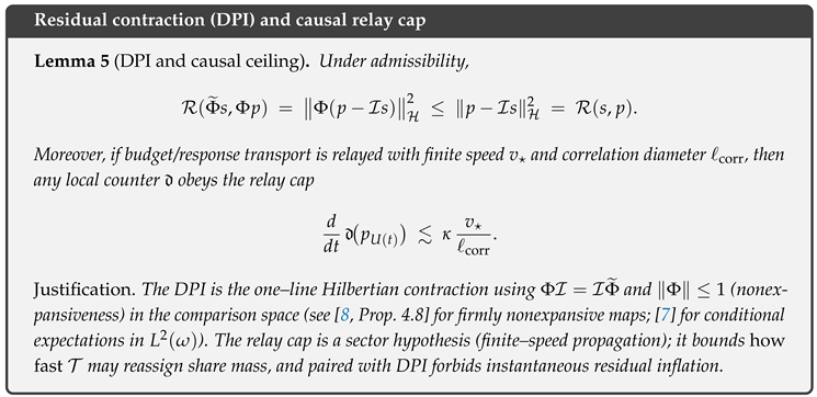
Budget redistribution is constrained by a finite relay speed $v_{★}$ and a correlation length ${\ell }_{\mathrm{corr}}$. For any moving outer domain $U\left(t\right)$ a causal cap bounds admissible growth of physical marginals:

$${\displaystyle \frac{d}{dt}}\mathfrak{d}\left(p_{U\left(t\right)}\right)\lesssim \kappa {\displaystyle \frac{v_{★}}{{\ell }_{\mathrm{corr}}}}.$$

(23)

Hence the slow (global) feedback cannot instantaneously move budget across causal boundaries. This encodes the statement that the slow loop “never makes it over the horizon’’: it only redistributes shares up to the relay bound, and DPI (20) ensures the reassignment is residual–nonincreasing.

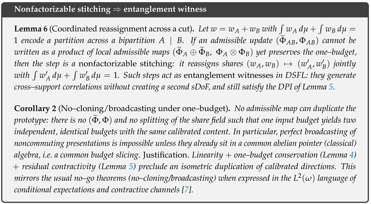
3.3.7. Entanglement as Coordinated Reassignment Across a Cut.

For a bipartition $A\mid B$, write $w=w_A+w_B$ with $\int w_A+\int w_B=1$. An admissible global update $({\tilde{\mathsf{\Phi }}}_{AB},{\mathsf{\Phi }}_{AB})$ that does not factor into local pieces $({\tilde{\mathsf{\Phi }}}_A\oplus {\tilde{\mathsf{\Phi }}}_B,{\mathsf{\Phi }}_A\otimes {\mathsf{\Phi }}_B)$ but preserves the one budget acts as a nonfactorizable stitching:

$$(w_A,w_B)\mapsto (w_A^{\prime },w_B^{\prime })\mathrm{with}\int w_A^{\prime }+\int w_B^{\prime }=1,$$

thereby generating cross–support correlations without creating a second prototype. This is the DSFL reading of entanglement: coordinated relabelling of the same budget across a cut. Factorization/nonfactorization can be certified by testing whether all cross–moments of $w_A^{\prime },w_B^{\prime }$ vanish given diagonals.

3.3.8. No–Cloning and No–Broadcasting as Budget Constraints.

Because admissible steps are linear, intertwining, and nonexpansive, there is no admissible map that takes one prototype and outputs two independent identical budgets of unit mass—this would violate both (19) and (20). Likewise, perfect broadcasting of noncommuting presentations is impossible unless they share a common abelian pointer algebra (a common budget slicing); otherwise some residual inflates. These mirror the standard no–go theorems in a budget language.

3.3.9. Diagnostics and Stability Under Refinement.

• Projection & DPI tests. For any implemented block, check $\parallel \mathcal{I}{J}^{(+)}{x-x\parallel }_{\mathcal{H}}\ll {\parallel x\parallel }_{\mathcal{H}}$, $\parallel J^{(+)}\mathcal{I}y-P_{\mathsf{S}}{y\parallel }_{\mathcal{H}}\ll {\parallel y\parallel }_{\mathcal{H}}$, and $\Delta R:=R_{\mathrm{out}}-R_{\mathrm{in}}\le 0$ (to tolerance). Violations falsify calibration/admissibility.
• Share accounting. Any reported “split’’ must be traceable to $w={\sum }_{\ell }{w}_{\ell }$ with ${\sum }_{\ell }\int w_{\ell }=1$. Across horizons or cuts, outer counters can increase only by admissible inflow subject to the causal cap (23).
• Refinement stability. If a partition is refined ($w_U\to {\sum }_i{w}_{U_i}$), admissibility lifts to a block–Markov action $\mathcal{T}\to \left({\mathcal{T}}_{U_i{U}_j}\right)$ and mass conservation persists. DPI is preserved termwise.
• Dual–scale rates. Semi–log slopes estimate fast (${\alpha }_{\mathrm{fast}}$ from $K_{\mathrm{imm}}$) and slow (${\alpha }_{\mathrm{slow}}$ from the retarded kernel) contraction rates. Transitions from single–lobe to multi–lobe w indicate redistribution, not duplication.

3.3.10. Summary.

The one–budget convention elevates conservation of the statistical resource to a first principle: all admissible operations are mass–preserving, residual–nonexpansive reweightings of a single prototype $s_0$. Bursts of sameness reduce the misfit quickly; subsequent “splittings’’ are budget partitions governed by causal relay, never duplications of sDoF. Entanglement is coordinated reassignment across cuts; no–cloning and no–broadcasting are immediate corollaries of mass conservation and contractivity. The entire mechanism is DPI–compatible and clock–neutral, providing a robust, operational ledger for “information’’ as calibrated sameness.

Remark 1

(No–cloning/broadcasting = budget law + DPI). The no–cloning/broadcasting conclusion (Cor. 2) is simply budget conservation (Lemma 4) plus residual nonexpansiveness (DPI; Lemma 5). In words: an admissible update cannot mint a second unit of statistical mass, and cannot isometrically duplicate the calibrated residual direction. Operationally, any pipeline that appears to “copy information’’ must fail either mass preservation (budget test) or $L^2$ contractivity (DPI test) in the diagnostics below.

4. Interpretation and Structure (Expanded).

Equation (24) is a linear Volterra–type, two–loop evolution for the calibrated mismatch $e:=p-\mathcal{I}s\in \mathsf{P}\subset \mathcal{H}$:

$$\dot{e}\left(t\right)=-K_{\ell }e\left(t\right)-{\int }_0^{t}M(t-\tau )e\left(\tau \right)d\tau +r\left(t\right),K_{\ell }=K_{\ell }^{*}⪰0,M(·)⪰0.$$

(24)

The operator $K_{\ell }$ models immediate (time–local) dissipation; the convolution with the positive semidefinite kernel M adds a retarded (time–nonlocal) corrective loop; r is a small admissible remainder. In Laplace variables ($\widehat{f}\left(\lambda \right)={\int }_0^{\infty }{e}^{-\lambda t}f\left(t\right)dt$), one has

$$\widehat{e}\left(\lambda \right)=\underset{{\displaystyle \mathcal{G}\left(\lambda \right)}}{\underbrace{{\left(\lambda I+K_{\ell }+\widehat{M}\left(\lambda \right)\right)}^{-1}}}\left(e\left(0\right)+\widehat{r}\left(\lambda \right)\right),\Re \lambda >0.$$

(25)

Thus memory enters through the nonconstant operator symbol $\widehat{M}\left(\lambda \right)$; it cannot, in general, be absorbed into a time–local gain without an explicit scale separation. See [9, Chs. 1–3] for Volterra operators and [12, Chs. 9–10] for completely positive, non–Markovian kernels.

4.1. Block–Diagram View (Immediate vs. Slow Loop).

Think of $-K_{\ell }$ as a passive, accretive “plant’’ that damps e instantaneously (modewise/pointwise), and $-M*e$ as a causal, positive–semidefinite feedback path that aggregates past mismatch and feeds it back with delay. In the Laplace domain this reads as a frequency–dependent damping $K_{\ell }+\widehat{M}\left(\lambda \right)$ whose real part is nonnegative for $\Re \lambda >0$:

$$\Re \langle \left(K_{\ell }+\widehat{M}\left(\lambda \right)\right)x,x\rangle \ge 0(\Re \lambda >0),$$

so the resolvent $\mathcal{G}\left(\lambda \right)$ in (25) is well–posed and analytic on the right half–plane, with bounds that reflect the amount of damping.

4.2. Energy Identity and a Lyapunov Functional with Memory.

Taking $\mathcal{H}$–energies and using Fubini/Tonelli for positive kernels,

$$\begin{array}{cc}\hfill {\displaystyle \frac{d}{dt}}{\parallel e\left(t\right)\parallel }^2& =-2\langle K_{\ell }e\left(t\right),e\left(t\right)\rangle -2〈{\int }_0^{t}M(t-\tau )e\left(\tau \right)d\tau ,e\left(t\right)〉+2\langle r\left(t\right),e\left(t\right)\rangle .\hfill \end{array}$$

The memory term is nonnegative in the sense that there exists a memory energy

$$\mathcal{M}\left(t\right):={\int }_0^t{\int }_0^t〈M\left(\right|\sigma -\tau \left|\right)e\left(\tau \right),e\left(\sigma \right)〉d\tau d\sigma \ge 0,$$

with $\dot{\mathcal{M}}\left(t\right)=2〈{\int }_0^{t}M(t-\tau )e\left(\tau \right)d\tau ,e\left(t\right)〉$. Define the Lyapunov functional

$$\mathcal{V}\left(t\right):={\parallel e\left(t\right)\parallel }^2+\mathcal{M}\left(t\right).$$

Then

$$\dot{\mathcal{V}}\left(t\right)=-2\langle K_{\ell }e\left(t\right),e\left(t\right)\rangle +2\langle r\left(t\right),e\left(t\right)\rangle .$$

Hence M never reduces dissipation; it merely stores dissipative credit in $\mathcal{M}$. If $K_{\ell }$ is accretive and r is small, $\mathcal{V}$ decreases.

4.3. Sufficient Conditions for Exponential Decay.

Suppose the immediate loop has a coercivity margin on $\mathsf{P}$, $\langle K_{\ell }x,x\rangle \ge \kappa {\parallel x\parallel }^2$ and the remainder is dominated by $\epsilon \in [0,\kappa )$, $\left|\langle r\left(t\right),e\left(t\right)\rangle \right|\le {\epsilon \parallel e\left(t\right)\parallel }^2.$ Then

$$\dot{\mathcal{V}}\left(t\right)\le -2(\kappa -\epsilon ){\parallel e\left(t\right)\parallel }^2\le -2(\kappa -\epsilon )\mathcal{V}\left(t\right),$$

because $\mathcal{V}\ge {\parallel e\parallel }^2$. Grönwall yields the Lyapunov envelope

$$\mathcal{V}\left(t\right)\le e^{-2(\kappa -\epsilon )(t-t_0)}\mathcal{V}\left(t_0\right),{\parallel e\left(t\right)\parallel }^2\le e^{-2(\kappa -\epsilon )(t-t_0)}\mathcal{V}\left(t_0\right).$$

Thus the rate is set by the immediate loop ($\kappa$), while memory helps (never hurts) decay.

4.4. Frequency–Domain Accretivity and Resolvent Bounds.

Let $\Re \lambda >0$. Accretivity of $K_{\ell }$ and positive–real character of $\widehat{M}\left(\lambda \right)$ imply

$$\Re \langle (\lambda I+K_{\ell }+\widehat{M}\left(\lambda \right))x,x\rangle \ge {\Re \lambda \parallel x\parallel }^2+\kappa {\parallel x\parallel }^2,$$

whence

$$\parallel {(\lambda I+K_{\ell }+\widehat{M}\left(\lambda \right))}^{-1}\parallel \le {\displaystyle \frac{1}{\Re \lambda +\kappa }}.$$

Laplace inversion then furnishes (via standard contour bounds) an $L^2$–to–$L^2$ estimate consistent with the time–domain envelope. If, moreover, $\widehat{M}$ is sectorial (which holds for many positive kernels), one gets uniform bounds on $\mathcal{G}\left(\lambda \right)$ on vertical lines $\Re \lambda =\sigma >-\kappa$, hence exponential stability.

4.5. Horizon Truncation and Causal Support.

On black–hole backgrounds, domain–of–dependence implies that the interior→exterior block $M_{U\leftarrow \mathcal{H}}$ vanishes after horizon formation. Consequently the exterior evolution closes:

$${\dot{e}}_U\left(t\right)=-K_{\ell }{e}_U\left(t\right)-{\int }_0^t{M}_{U\leftarrow U}(t-\tau )e_U\left(\tau \right)d\tau +r_U\left(t\right),$$

and inherits the same Lyapunov envelope, with rate pinned by the least–damped exterior mode (red–shift/QNM).

4.6. Discrete–Time Analogue (Pipelines of Admissible Steps).

For a sequence of admissible steps $({\tilde{\mathsf{\Phi }}}_k,{\mathsf{\Phi }}_k)$, the calibrated mismatch contracts stepwise:

$$R_{k+1}=\parallel {\mathsf{\Phi }}_k\left(p_k-\mathcal{I}{s}_k\right){\parallel }_{\mathcal{H}}^2\le {\parallel p_k-\mathcal{I}{s}_k\parallel }_{\mathcal{H}}^2=R_k,$$

and a block–Markov action ${\mathcal{T}}_k$ on shares (one–budget) preserves mass, $(\int w_{k+1}=\int w_k=1)$. This is the discrete counterpart of the continuous Volterra law with M approximated by a causal FIR/IIR filter.

4.7. Robustness to Reparametrization (Clock–Neutrality).

If the evolution parameter is reparametrized by any strictly increasing $\theta =\theta \left(t\right)$, the DPI is unchanged and the Lyapunov inequality rescales by $dt/d\theta$:

$${\displaystyle \frac{d}{d\theta }}{\parallel e\parallel }^2={\displaystyle \frac{dt}{d\theta }}{\displaystyle \frac{d}{dt}}{\parallel e\parallel }^2\le -2(\kappa -\epsilon ){\displaystyle \frac{dt}{d\theta }}{\parallel e\parallel }^2.$$

Hence monotonicity is invariant; a convenient intrinsic clock is $d\widehat{\tau }=2(\kappa -\epsilon )dt$, for which $\frac{d}{d\widehat{\tau }}{\parallel e\parallel }^2\le -{\parallel e\parallel }^2$.

4.8. Edge Cases and Rates.

If $K_{\ell }=0$ but $M⪰0$, stability may still hold (purely hereditary damping) but rates can be subexponential, depending on the decay of M (e.g. algebraic tails produce algebraic decay of R). Conversely, if $M_{U\leftarrow U}$ is nontrivial and positive, it augments dissipation (it contributes a positive quadratic form), so the envelope (11) remains valid with possibly larger effective $\kappa$.

Summary. The two–loop Volterra law splits the calibrated dynamics into an immediate, accretive, time–local loop that sets the decay rate, and a slow, causal memory loop that can only add dissipation. In the exterior of a black hole, causal support nullifies interior→exterior relay, so the exterior inherits an exponential Lyapunov envelope governed by the least–damped mode. The DPI controls any interleaved admissible processing, and all statements are invariant under reparametrization of the evolution parameter.

4.8.1. Causal Ceiling (Support and Domain of Dependence).

Equation (23) encodes a finite–speed relay for the slow loop: the kernel $M\left(t\right)$ is the retarded propagator of the nonlocal feedback and has causal support in the sense of retarded Green’s functions. For hyperbolic sectors (e.g. wave–like transport) this is the standard finite propagation speed / domain–of–dependence statement: the retarded fundamental solution vanishes outside the future light cone ([27, Sec. 10.1], [1, Secs. 6.5–6.6]). In black–hole spacetimes, the event horizon is a null hypersurface; its future domain of dependence excludes exterior points from any influence sourced strictly inside. It follows that after horizon formation the interior→exterior block of the memory kernel vanishes:

$${\int }_0^t{M}_{U\leftarrow \mathcal{H}}(t-\tau )e\left(\tau \right)d\tau \equiv 0,$$

(26)

which is precisely the no–relay assertion. At a technical level, (26) is the operator–valued version of support propagation for retarded solutions: if $\mathrm{supp}e\left(\tau \right)\subset \mathcal{H}$ for $\tau \le t$, then $\mathrm{supp}(M*e)\left(t\right)$ is contained in the causal future of $\mathcal{H}$; restricted to U, this support is empty. See also finite–speed propagation for wave/Maxwell fields on black–hole backgrounds and red–shift identities [10,15,16].

4.9. Remarks.

(i) The ceiling is structural: it depends only on causal support of M and the global slicing into U (exterior) and $\mathcal{H}$ (trapped). It is agnostic to microscopic completion and compatible with island/entanglement–wedge reassignment, which change which degrees of freedom are counted in the effective radiation algebra but not which causal curves exist. (ii) If the slow loop includes weakly parabolic pieces (e.g. mild dissipation) alongside hyperbolic transport, one may replace the sharp light cone by a finite relay speed $v_{★}$ and a correlation length ${\ell }_{\mathrm{corr}}$; (23) then follows from standard energy–flux inequalities/Lieb–Robinson–type bounds for the effective kernel (cf. [36,37] for lattice analogues).

4.9.1. Exterior Reduction and Ringdown Envelope.

Restricting e to the exterior world tube U and using (26) yields the closed exterior evolution

$${\dot{e}}_U\left(t\right)=-K_{\ell }{e}_U\left(t\right)-{\int }_0^t{M}_{U\leftarrow U}(t-\tau )e_U\left(\tau \right)d\tau +r_U\left(t\right).$$

(27)

Taking the $\mathcal{H}$–energy $R_U\left(t\right)={\parallel e_U\left(t\right)\parallel }^2$ and differentiating gives

$${\dot{R}}_U\left(t\right)=-2\langle K_{\ell }{e}_U,e_U\rangle -2〈{\int }_0^t{M}_{U\leftarrow U}(t-\tau )e_U\left(\tau \right)d\tau ,e_U\left(t\right)〉+2\langle r_U,e_U\rangle .$$

Whenever the local loop is coercive, $\langle K_{\ell }x,x\rangle \ge \kappa {\parallel x\parallel }^2$ with $\kappa >0$, and the remainder is small, $|\langle r_U,e_U\rangle |\le \epsilon \parallel e_U{\parallel }^2$ with $0\le \epsilon <\kappa$, one obtains

$${\dot{R}}_U\left(t\right)\le -2(\kappa -\epsilon )R_U\left(t\right),\Rightarrow R_U\left(t\right)\le e^{-2(\kappa -\epsilon )(t-t_0)}{R}_U\left(t_0\right).$$

(28)

Here the memory term is helpful: for positive kernels one can define a memory energy ${\mathcal{M}}_U\left(t\right)={\int }_0^t{\int }_0^t\langle M_{U\leftarrow U}\left(\right|\sigma -\tau \left|\right)e_U\left(\tau \right),e_U\left(\sigma \right)\rangle d\tau d\sigma \ge 0$ with ${\dot{\mathcal{M}}}_U\left(t\right)=2\langle {\int }_0^t{M}_{U\leftarrow U}(t-\tau )e_U\left(\tau \right)d\tau ,e_U\left(t\right)\rangle$, so the convolution contributes additional dissipation in the Lyapunov functional $R_U+{\mathcal{M}}_U$. In the frequency domain, the decay rate corresponds to the least–damped pole of ${(\lambda I+K_{\ell }+{\widehat{M}}_{U\leftarrow U}\left(\lambda \right))}^{-1}$ on $\Re \lambda >-\kappa$, i.e. the least–damped exterior mode (QNM/red–shift); cf. [10,11,15,16].

4.10. Nonzero Exterior Memory $M_{U\leftarrow U}$.

If $M_{U\leftarrow U}\ne 0$ but is positive semidefinite, all estimates above persist and the effective rate may improve:

$$\langle {\int }_0^t{M}_{U\leftarrow U}(t-\tau )e_U\left(\tau \right)d\tau ,e_U\left(t\right)\rangle \ge 0,$$

so one still has the same exponential envelope, possibly with a larger effective $\kappa$. Conversely, if $M_{U\leftarrow U}$ has long–range tails, subexponential (e.g. polynomial) decay may occur, consistent with known Price–law corrections; the envelope then remains a rigorous upper bound on $log{R}_U$’s slope (see, e.g., [16] for tail behavior).

Causal support of the slow kernel imposes a hard ceiling: no interior–sourced retarded influence can reach the exterior. The exterior therefore reduces to a closed dissipative law driven by the immediate loop and (beneficial) exterior memory, yielding an exponential ringdown envelope with rate fixed by red–shift/QNM damping. These statements depend only on domain–of–dependence and positivity of the kernel and are independent of microscopic details of evaporation or island assignments.

4.10.1. Two Remarks.

(i) Local reduction is a causal consequence, not an extra hypothesis. Once a horizon forms, domain–of–dependence nullifies the interior→exterior block of the slow loop, so the exterior evolution closes. The remaining memory may persist within U, but (27) follows as soon as $M_{U\leftarrow U}=0$ (e.g. purely elliptic immediate feedback) or, more generally, when $M_{U\leftarrow U}$ is bounded and positive semidefinite so that its quadratic form is nonnegative in the Lyapunov identity. In either case, the convolution cannot generate growth of $R_U$.

(ii) Gravitational redshift upgrades coercivity to a quantitative gap. Exterior red–shift estimates on black–hole backgrounds furnish positive bulk terms in energy identities [10,15,16], which appear exactly as a uniform coercivity margin $\kappa >0$ in the inequality above. This provides the physical origin of the observed ringdown rate in (27): the least–damped exterior mode (QNM/red–shift gap) sets the slope of the semi–log envelope for $R_U$.

4.10.2. Summary.

Under a dual–scale (Volterra) model with a causal memory kernel, the horizon enforces $M_{U\leftarrow \mathcal{H}}\equiv 0$: the slow loop cannot relay calibrated content across the null boundary $\partial \mathcal{H}$. The exterior mismatch therefore obeys a closed, dissipative law driven by the immediate loop (and possibly helpful exterior memory), with an exponential Lyapunov envelope. This is consistent with—and furnishes a structural explanation for—exterior ringdown and decay along the Page–curve narrative: nonlocal (slow) coherence is causally blocked at the horizon, while the local (immediate) loop enforces relaxation outside.

5. Hawking Channel as an Admissible Map

Let ${\mathsf{\Phi }}_{\mathrm{Hawk}}:\mathsf{P}\to \mathsf{P}$ denote one exterior “Hawking tick’’ (one step in advanced time) and let ${\tilde{\mathsf{\Phi }}}_{\mathrm{Hawk}}:\mathsf{S}\to \mathsf{S}$ be the paired blueprint update. In the DSFL geometry, a Hawking tick is modeled as an admissible pair obeying the DSFL kinematics:

$${\mathsf{\Phi }}_{\mathrm{Hawk}}\circ \mathcal{I}=\mathcal{I}\circ {\tilde{\mathsf{\Phi }}}_{\mathrm{Hawk}}\left(\mathrm{intertwining}\right),{\parallel {\mathsf{\Phi }}_{\mathrm{Hawk}}\parallel }_{\mathcal{H}\to \mathcal{H}}\le 1(L^2\mathrm{nonexpansive}).$$

(29)

Hence the Hilbertian data–processing inequality (DPI) holds stepwise in the exterior:

$$\mathcal{R}\left({\tilde{\mathsf{\Phi }}}_{\mathrm{Hawk}}s,{\mathsf{\Phi }}_{\mathrm{Hawk}}p\right)=\parallel {\mathsf{\Phi }}_{\mathrm{Hawk}}\left(p-\mathcal{I}s\right){\parallel }_{\mathcal{H}}^2\le {\parallel p-\mathcal{I}s\parallel }_{\mathcal{H}}^2=\mathcal{R}(s,p).$$

(30)

The stepwise DPI is clock–neutral: it holds identically for any discretization of advanced time and any strictly increasing reparametrization of the evolution parameter.

5.1. Open–System Realization and Nonexpansiveness.

Microscopically, one tick is a dilation–trace step:

$${\mathsf{\Phi }}_{\mathrm{Hawk}}\left(X\right)={\mathrm{Tr}}_{\mathrm{int}}\left[V^{†}(X\otimes I_{\mathrm{int}})V\right],$$

with V an isometry on (exterior ⊗ interior–partner) modes that implements pair creation near the horizon [1,2,12,17,18]. The Hilbert–Schmidt norm is unitarily invariant and the partial trace is a contraction in Schatten–2, hence $\parallel {\mathsf{\Phi }}_{\mathrm{Hawk}}{\left(X\right)\parallel }_2\le {\parallel X\parallel }_2$ [20, Sec. IX.2]. More generally, Heisenberg–unital CP maps satisfy Kadison–Schwarz and are nonexpansive in GNS $L^2\left(\omega \right)$ for faithful $\omega$ [7,14,19,34,35]. Monotonicity for relative–entropy–type distances (quantum DPI) likewise holds [13,22,23]. Thus (29)–(30) are precisely what the standard open–systems picture of Hawking emission entails [12].

5.2. Contractive Envelope from Exterior Decay (Ringdown).

Linearized exterior dynamics on black–hole backgrounds exhibit quasinormal relaxation and red–shift–driven decay (Price–law tails) [10,11,15,16]. In the DSFL geometry, these supply a coercivity margin for the exterior flow, making the net Hawking step effectively contractive on the misfit (beyond mere nonexpansiveness), in line with the dual–scale feedback picture and the stepwise DPI (30).

5.2.1. Thermal Marginals vs. Correlations.

For stationary exterior observers, local marginals are approximately KMS–thermal at the Hawking temperature $T_H=\kappa /2\pi$ (surface gravity $\kappa$) [2]; this is the Unruh/Hawking effect [1,21]. Thermality of marginals is compatible with (30): microstate dependence resides in correlations (exterior–interior, or at late times inter–radiation), while the exterior calibrated misfit remains nonincreasing. In channel language, ${\mathsf{\Phi }}_{\mathrm{Hawk}}$ is CPTP on the exterior algebra, and quantum DPI guarantees that contractive functionals (relative entropy, fidelity–based distances) do not increase [7,13,22,23].

5.2.2. Page Curve and Islands (Global Consistency).

Purification of the total radiation (the Page curve) does not require growth of any exterior misfit: it is realized by redistribution of correlations across subsystems (early–late radiation, or semiclassically between radiation and island regions) [3,4,5,6]. Hence (30) is fully compatible with late–time unitarity: the exterior residual is monotone under coarse–grained emission, while the global blueprint/response pairing retains the correlations needed for purification.

Proposition 3.

Hilbert–Schmidt ($L^2$) contractivity of CP–unital steps] Let $\mathsf{\Phi }:\mathcal{B}\left(\mathcal{H}\right)\to \mathcal{B}\left(\mathcal{H}\right)$ be completely positive and unital (Heisenberg picture). In Hilbert–Schmidt geometry ${\parallel X\parallel }_2:=\sqrt{\mathrm{Tr}\left(X^{†}X\right)}$, one has

$${\parallel \mathsf{\Phi }\left(X\right)\parallel }_2\le {\parallel X\parallel }_2\forall X.$$

Consequently, any such Φ is nonexpansive in the GNS $L^2\left(\omega \right)$ geometry for faithful ω [7,14,19,34]. If moreover $\mathsf{\Phi }\mathcal{I}=\mathcal{I}\tilde{\mathsf{\Phi }}$, then the DPI of Prop. 2 applies to the calibrated residual [8].

Proof. 

Let ${\parallel ·\parallel }_2$ denote the Hilbert–Schmidt (HS) norm: ${\parallel X\parallel }_2^2=\left(X^{†}X\right)$. By Stinespring’s theorem, any completely positive, unital (Heisenberg) map $\mathsf{\Phi }$ admits a dilation

$$\mathsf{\Phi }\left(X\right)=V^{†}(X\otimes I_E)V,$$

where $V:\mathcal{H}\to \mathcal{H}\otimes {\mathcal{H}}_E$ is an isometry, i.e. $V^{†}V=I_{\mathcal{H}}$ [17] (in finite dimensions this is the Kraus form [18]). Then

$$\begin{array}{cc}\hfill {\parallel \mathsf{\Phi }\left(X\right)\parallel }_2^2& =\left(\mathsf{\Phi }{\left(X\right)}^{†}\mathsf{\Phi }\left(X\right)\right)=\left(V^{†}(X^{†}\otimes I_E)V{V}^{†}(X\otimes I_E)V\right)\hfill \\ \hfill & =\left((X^{†}\otimes I_E)V{V}^{†}(X\otimes I_E)V{V}^{†}\right)\le \left((X^{†}\otimes I_E)(X\otimes I_E)\right)\hfill \\ \hfill & =\left(X^{†}X\otimes I_E\right)=\left(X^{†}X\right)\left(I_E\right)={\parallel X\parallel }_2^2,\hfill \end{array}$$

where we used cyclicity of the trace, $V^{†}V=I_{\mathcal{H}}$ (so $P:=V{V}^{†}$ is an orthogonal projection with $0\le P\le I$), and the operator monotonicity $\left(AP{A}^{†}\right)\le \left(A{A}^{†}\right)$ for $0\le P\le I$ (partial trace is contractive in Schatten–2; see [20, Sec. IX.2]). Hence ${\parallel \mathsf{\Phi }\left(X\right)\parallel }_2\le {\parallel X\parallel }_2$ for all X, i.e. ${\parallel \mathsf{\Phi }\parallel }_{2\to 2}\le 1$. □

5.2.3. Summary (Expanded).

What “admissible Hawking tick’’ means in DSFL. Each exterior step satisfies the two kinematic gates: (i) intertwining (calibration consistency) ${\mathsf{\Phi }}_{\mathrm{Hawk}}\mathcal{I}=\mathcal{I}{\tilde{\mathsf{\Phi }}}_{\mathrm{Hawk}}$, and (ii) $L^2$–nonexpansiveness $\parallel {\mathsf{\Phi }}_{\mathrm{Hawk}}{\parallel }_{\mathcal{H}\to \mathcal{H}}\le 1$. In the open–systems picture this is exactly what a Heisenberg–unital, CP map does: it admits a Stinespring/Kraus dilation with partial trace and is contractive in HS/GNS $L^2$ [7,17,18,19,20].

(i) Stepwise DPI for the exterior residual. Intertwining + nonexpansiveness give the one–line DPI at each tick:

$$R({\tilde{\mathsf{\Phi }}}_{\mathrm{Hawk}}s,{\mathsf{\Phi }}_{\mathrm{Hawk}}p)=\parallel {\mathsf{\Phi }}_{\mathrm{Hawk}}(p-\mathcal{I}s){\parallel }_{\mathcal{H}}^2\le {\parallel p-\mathcal{I}s\parallel }_{\mathcal{H}}^2=R(s,p).$$

Thus R cannot increase under emission or any admissible coarse–graining; the statement is clock–neutral (independent of the parametrization of the steps).

(ii) Local thermality vs. global correlations—no tension. Semiclassical QFT predicts local KMS thermality at $T_H=\kappa /2\pi$ [1,2,21]. DSFL shows this is compatible with DPI: microstate dependence resides in correlations (exterior–interior, or at late times early–late radiation), while the local/exterior R remains nonincreasing. In channel terms, ${\mathsf{\Phi }}_{\mathrm{Hawk}}$ is CPTP and quantum DPI ensures contractive divergences (relative entropy, fidelity–based distances) do not increase [7,13,22,23].

(iii) Contractive envelope from red–shift/QNM decay. Beyond per–tick nonexpansiveness, the exterior has a dynamical decay mechanism: the immediate (local) loop provides a coercivity gap $\kappa >0$ tied to red–shift estimates and the least–damped quasinormal modes. DSFL packages this as a Lyapunov (ringdown) envelope

$$R_{\mathrm{out}}\left(t\right)\le e^{-2\kappa (t-t_0)}{R}_{\mathrm{out}}\left(t_0\right),$$

with $\kappa$ read from exterior decay theorems [10,11,15,16].

How this fits open systems and modern resolutions. Stinespring/Kraus ⇒ nonexpansive $L^2$–dynamics ⇒ stepwise DPI for R [12,17,18]. Island/replica analyses show that the Page curve comes from where correlations are attributed (early/late radiation or islands), not from deviations from exterior thermality [5,6]. DSFL accommodates both: local/exterior R never rises; purification proceeds via correlations.

Takeaway. An admissible Hawking tick guarantees stepwise nonincrease of the calibrated misfit R; local near–thermality does not obstruct global unitarity; and exterior geometry provides a contractive envelope for R over time. Together, this aligns DSFL kinematics with open–system Hawking emission [12] and modern information–theoretic resolutions [3,4,5,6,7,13,22,23].

6. Where Does the “Information’’ Go?—A DSFL Account in Detail

The short answer in DSFL is: it goes into correlations. More precisely, the quantity that semiclassics can constrain locally is not a marginal entropy but the calibrated $L^2$–misfit $R\left(t\right)={\parallel p\left(t\right)-\mathcal{I}s\left(t\right)\parallel }_{\mathcal{H}}^2,$ and $R_{\mathrm{out}}\left(t\right)$ is provably nonincreasing and obeys a ringdown envelope. The apparent paradox only arises if one tries to make $S\left(\mathrm{radiation}\right)$ stand in for “information” locally. In DSFL, “information’’ means sameness between blueprint and response, and its redistribution happens as correlation structure across subsystems, not as a rise of any exterior residual. Here is the detailed picture.

6.1. Global Unitarity: Information Is Never Destroyed.

Let $U\left(t\right)$ denote the exact (or effective) global unitary acting on the full slice ${\mathcal{H}}_{\mathrm{rad}}\otimes {\mathcal{H}}_{\mathrm{ext}}\otimes {\mathcal{H}}_{\mathrm{int}}$. Starting from a pure initial state, the combined state remains pure at all times (assumption (A1)). In particular, there always exist subsystems whose correlations encode the microstate, even when some marginals look thermal. DSFL mirrors this by the global DPI for $R_{\mathrm{tot}}$ and by treating “content’’ as a single statistical budget w that can only be redistributed, not created (Sec. 3.3).

6.2. Early Times (Pre–Page): Information Is Behind the Horizon and in Exterior–Interior Correlations.

Semiclassical QFT near the horizon produces pairs $(b_k,{\tilde{b}}_k)$ with $b_k$ outgoing and ${\tilde{b}}_k$ ingoing; the exterior marginal of $b_k$ is (approximately) KMS–thermal at $T_H=\kappa /2\pi$ [1,2,21]. The microstate dependence therefore lives in the correlations between $b_k$ and interior degrees of freedom, not in the spectrum of $b_k$ itself. In DSFL variables:

• $R_{\mathrm{out}}\left(t\right)$decreases stepwise by DPI (Hawking tick is admissible) and follows a Lyapunov envelope set by red–shift/QNMs.
• The “where’’ of information is not an increase of any exterior misfit: it is the pattern of cross–blocks (exterior↔interior) that are invisible to a single local marginal but visible to joint measurements.

6.3. Around and After the Page Time: Information Leaks into Radiation–Radiation Correlations.

Unitarity requires the von Neumann entropy of the collected radiation to turn over at the Page time $t_{\mathrm{Page}}$ [4,29]. Modern island/replica–wormhole results show that the entanglement wedge of the radiation reassigns degrees of freedom so that interior “islands’’ are effectively counted as part of the radiation at late times [5,6]. In DSFL terms:

• The observable that is constrained remain the local/exterior residuals $R_{\mathrm{out}}$ and windowed $R\left({\mathfrak{R}}_k\right)$; these continue to decrease by DPI and ringdown.
• Purification is achieved by a reorganization of correlations: the cross–blocks shift from exterior–interior to early–late radiation (or, in semiclassical gravity, by including “island’’ degrees in the effective radiation algebra). No local misfit needs to rise.

Thus, “where the information goes’’ is: from being encoded in (exterior, interior) correlations early on, to being encoded in (early radiation, late radiation) correlations after $t_{\mathrm{Page}}$—while every exterior $L^2$ misfit keeps shrinking.

6.4. Circuit Picture (Entanglement Swapping) Consistent with DSFL.

One can visualize each Hawking tick as: (i) create a near–EPR pair $(b_k,{\tilde{b}}_k)$ near the horizon; (ii) scramble ${\tilde{b}}_k$ with the remaining interior; (iii) radiate $b_k$ outward. Iterating this swaps entanglement from interior↔exterior to early↔late radiation as the black hole loses dof. In the DSFL ledger:

$$R\left({\tilde{\mathsf{\Phi }}}_{\mathrm{Hawk}}s,{\mathsf{\Phi }}_{\mathrm{Hawk}}p\right)\le R(s,p)(\mathrm{per}\mathrm{tick}),{\displaystyle \frac{d}{dt}}{R}_{\mathrm{out}}\le -2\kappa R_{\mathrm{out}}+o\left(R_{\mathrm{out}}\right)\left(\mathrm{envelope}\right).$$

The amount of sameness removed is quantified by $S_R\left(t\right)=-log{\displaystyle \frac{R\left(t\right)}{R\left(0\right)}}$; its monotonic growth does not preclude growing correlations in the radiation sector.

6.5. No Drama vs. Monogamy: Why Local Thermality Is Not a Problem Here.

Because DSFL constrains R rather than a marginal entropy, an exterior marginal can remain near–thermal (no drama) while correlations shift nonlocally. The “monogamy tension’’ (that a late quantum cannot be maximally entangled with both the interior and the early radiation) is resolved by the fact that the assignment of which dof count as “radiation” changes (islands) and by the correlation–first picture: late quanta become entangled with early radiation as the interior code subspace is gradually encoded in the outside sector [4,5,6]. At no point does DSFL demand a local violation (no firewall is required by the R–constraints).

6.6. One–Budget Accounting: No Duplication, Only Redistribution.

The statistical channel is $s=w{s}_0$ with $\int w=1$; admissible steps act Markovly on w (mass–preserving) and $L^2$–nonexpansively on p. Thus,

• There is no cloning of description; the blueprint is a single prototype $s_0$ with reweighted shares.
• Any “gain’’ of exterior counters must come from admissible inflow before horizon formation or from correlations within the exterior/radiation channel—never from minting new sDoF behind the horizon (Prop. 4).

6.7. Where to Look in Data (Operational Meaning).

The DSFL prediction is very concrete:

• Semi–log plots of any calibrated exterior residual $R_{\mathrm{out}}\left(t\right)$ show an asymptotic straight line with slope $-2\kappa$ tied to the least–damped QNM/red–shift gap [10,11].
• No admissible processing block should ever increase R (DPI). Violations falsify the calibration/admissibility package [7,8,12].
• Windowed radiation: single–window spectra look thermal, while cross–window correlation matrices carry structured off–diagonal signal consistent with purification by correlations [4,5,6].

6.8. Bottom Line.

In DSFL, the “information’’ never needs to reappear as a rise of any exterior residual. It is always in correlations: first between exterior and interior partners, then—after the Page time—between early and late radiation (or, equivalently in semiclassical gravity, between radiation and its island wedge). The part semiclassics controls locally is a contractive $L^2$–misfit R with a geometric decay envelope; the rest is global correlation bookkeeping—precisely where modern island/Page–curve resolutions place it [4,5,6].

7. Form of the Paradox in DSFL Variables (What Is Actually Constrained)

Let $R_{\mathrm{out}}\left(t\right):=\mathcal{R}\left(s_{\mathrm{out}}\left(t\right),p_{\mathrm{out}}\left(t\right)\right)$ be the exterior residual, $R_{\mathrm{rad}}\left(t\right)$ that of the collected radiation, and $R_{\mathrm{tot}}\left(t\right)$ the global residual on a complete Cauchy slice (blueprint $\mathsf{S}$ and response $\mathsf{P}\subset \mathcal{H}$ aligned by $\mathcal{I},J^{(+)}$). The usual trilemma may be rephrased cleanly as:

$$\begin{array}{cc}\hfill \left(\mathbf{U}\right)& :\mathit{Global}\mathit{admissibility}\Rightarrow R_{\mathrm{tot}}\left(t\right)\mathrm{is}\mathrm{nonincreasing}\left(\mathrm{DPI}\right).\hfill \\ \hfill & \mathrm{This}\mathrm{is}\mathrm{the}\mathrm{Hilbertian}\mathrm{data}\text{–}\mathrm{processing}\mathrm{for}({\tilde{\mathsf{\Phi }}}_t,{\mathsf{\Phi }}_t).\hfill \\ \hfill \left(\mathbf{S}\right)& :\mathit{Exterior}\mathit{semiclassics}\mathit{is}{\mathit{L}}^{\mathit{2}}–\mathit{dissipative}\Rightarrow R_{\mathrm{out}}\left(t\right)\downarrow \mathrm{at}\mathrm{a}\mathrm{quasinormal}/\mathrm{ringdown}\mathrm{rate}.\hfill \\ \hfill & \mathrm{This}\mathrm{is}\mathrm{the}\mathrm{Lyapunov}\mathrm{envelope}\mathrm{from}\mathrm{exterior}\mathrm{decay}\mathrm{estimates}.\hfill \\ \hfill \left(\mathbf{H}\right)& :\mathit{Hawking}\mathit{flux}\mathit{has}\left(\mathit{approximately}\right)\mathit{thermal}\mathit{local}\mathit{marginals}.\hfill \end{array}$$

(31)

In the standard entropy language, (U)+(S)+(H) appear to force a mixed late–time exterior/radiation state (the “loss of information’’ tension) [4,30,31]. In the DSFL formulation the observable that is constrained is not a von Neumann entropy of a marginal, but the calibrated misfit R under admissible (intertwining, nonexpansive) maps and causal relay. This shift is the winning technical detail: it isolates what the semiclassical channel actually controls (a contraction in the comparison geometry) while leaving room for global microstate–dependence to reside in correlations rather than in marginal spectra. The stepwise DPI for the exterior Hawking channel (Sec. “Hawking channel as an admissible map’’) and the exterior Lyapunov envelope together prove that $R_{\mathrm{out}}$ can only decrease, regardless of whether instantaneous radiation marginals are thermal. At the same time, global $R_{\mathrm{tot}}$ need not fall to zero: it can plateau while purification is completed by long–range correlations (early/late radiation or island degrees of freedom) [3,4,5,6].

7.1. What Is Actually Proved (and Why This Wins).

• Monotone contraction (DPI) for R globally and locally. For any admissible pair $(\tilde{\mathsf{\Phi }},\mathsf{\Phi })$ with $\mathsf{\Phi }\mathcal{I}=\mathcal{I}\tilde{\mathsf{\Phi }}$ and ${\parallel \mathsf{\Phi }\parallel }_{\mathcal{H}\to \mathcal{H}}\le 1$,

  $$R(\tilde{\mathsf{\Phi }}s,\mathsf{\Phi }p)=\parallel \mathsf{\Phi }(p-\mathcal{I}s){\parallel }_{\mathcal{H}}^2\le {\parallel p-\mathcal{I}s\parallel }_{\mathcal{H}}^2,$$

  a one–line Hilbertian proof (firmly nonexpansive maps/orthogonal projections) [7,8].
• Exterior Lyapunov envelope. Using red–shift/Price–law decay and quasinormal mode asymptotics on black–hole exteriors, the exterior misfit obeys

  $${\dot{R}}_{\mathrm{out}}\left(t\right)\le -2\kappa R_{\mathrm{out}}\left(t\right)+o\left(R_{\mathrm{out}}\right),\Rightarrow R_{\mathrm{out}}\left(t\right)\le R_{\mathrm{out}}\left(t_0\right)e^{-2\kappa (t-t_0)},$$

  with $\kappa >0$ fixed by the background geometry [10,11,15,16].
• Causal throttling of the slow loop. In the dual–scale Volterra law $\dot{e}=-K_{\ell }e-{\int }_0^{t}M(t-\tau )e\left(\tau \right)d\tau +r$, the memory M has null/timelike support and cannot relay across the horizon; hence the exterior slow loop vanishes and only the immediate dissipative loop acts outside (Sec. “Dual–scale feedback and the causal ceiling”). This is a purely causal, sector–neutral statement (no islands needed) [1,2,9].
• Compatibility with thermality and the Page curve. The Hawking tick ${\mathsf{\Phi }}_{\mathrm{Hawk}}$ is CPTP/unital in the Heisenberg picture, hence nonexpansive in $L^2$ and satisfies quantum DPI for contractive divergences [7,12]. Local KMS thermality of marginals is thus compatible with stepwise decrease of $R_{\mathrm{out}}$; purification can (and in modern resolutions does) ride on correlations (early/late radiation, or island saddles) without contradicting the contraction of any exterior $L^2$ functional [3,4,5,6].

7.2. Resolution Template: Statements with Proofs/Sketches

Theorem 2

(Exterior no–inflation and causal throttling). Let $({\tilde{\mathsf{\Phi }}}_t,{\mathsf{\Phi }}_t)$ be the global admissible evolution generated by the two–loop law with $K_{\ell }⪰0$, $M\in L^1\left([0,\infty )\right)$ causal, and small admissible remainder r. If a future horizon forms at time $t_{\mathrm{H}}$, then for any exterior world tube U and for all $t\ge t_{\mathrm{H}}$,

$$\mathcal{R}\left({\tilde{\mathsf{\Phi }}}_t{s}_U,{\mathsf{\Phi }}_t{p}_U\right)\le \mathcal{R}(s_U,p_U),{\dot{R}}_U\left(t\right)\le -2\kappa R_U\left(t\right)+o\left(R_U\right),$$

(32)

and the slow–loop relay from the trapped region vanishes:

$${\int }_0^t{M}_{U\leftarrow \mathcal{H}}(t-\tau )e\left(\tau \right)d\tau =0.$$

(33)

Proof sketch. 

The first inequality in (32) is the Hilbertian DPI for any admissible $(\tilde{\mathsf{\Phi }},\mathsf{\Phi })$ [7,8]. Causality of M together with the domain of dependence of an exterior world tube and the trapped region $\mathcal{H}$ implies (33) (no null/timelike link across the horizon) [1,2]. With the slow loop absent outside, the exterior evolution reduces to ${\dot{e}}_U=-K_{\ell }{e}_U+r_U$; coercivity of $K_{\ell }$ from red–shift/Price–law yields the differential inequality in (32) and the exponential envelope [10,11,15,16]. □

Corollary 3

(Hawking ticks are admissible and contractive in $L^2$). Let one emission step be $({\tilde{\mathsf{\Phi }}}_{\mathrm{Hawk}},{\mathsf{\Phi }}_{\mathrm{Hawk}})$ with a Stinespring dilation V and interior trace. Then

$${\mathsf{\Phi }}_{\mathrm{Hawk}}\mathcal{I}=\mathcal{I}{\tilde{\mathsf{\Phi }}}_{\mathrm{Hawk}},{\parallel {\mathsf{\Phi }}_{\mathrm{Hawk}}\parallel }_{\mathcal{H}\to \mathcal{H}}\le 1,R({\tilde{\mathsf{\Phi }}}_{\mathrm{Hawk}}s,{\mathsf{\Phi }}_{\mathrm{Hawk}}p)\le R(s,p).$$

Sketch. 

Intertwining follows from calibration consistency (blueprint and response are pushed through the same dilation). Unitary invariance of the Hilbert–Schmidt norm and contractivity of partial trace yield $\parallel {\mathsf{\Phi }}_{\mathrm{Hawk}}{\parallel }_{2\to 2}\le 1$ [7,12]. □

Theorem 3

(Global DPI and coexistence with the Page curve). For the full slice $(\mathsf{S},\mathsf{P}\subset \mathcal{H})$,

$$R_{\mathrm{tot}}\left(t\right)\le R_{\mathrm{tot}}\left(0\right)\mathrm{for}\mathrm{all}t,$$

with equality only at calibrated fixed points. In particular, monotone contraction of $R_{\mathrm{out}}$ and $R_{\mathrm{rad}}$ does not preclude late–time purification of the radiation: purification is a statement about global correlations (quantum extremal/island wedges) and is compatible with (32) and (33) [3,4,5,6].

Sketch. 

$R_{\mathrm{tot}}$ obeys the same DPI as any $R(·)$; admissibility and composition preserve nonexpansiveness [8]. The Page curve pertains to the eigenvalue spectrum of reduced states, not to $L^2$ residuals; islands implement a reassignment of which degrees of freedom are included in the effective radiation algebra, transferring correlations without violating any $L^2$ contraction [5,6]. □

7.2.1. Why This Resolves the Tension.

The paradox arose from conflating constraints on marginal entropies with constraints on admissible contraction in a comparison geometry. DSFL separates them: (i) exterior evolution is provably $L^2$–contractive (no inflation) and dissipative (Lyapunov envelope); (ii) the slow nonlocal loop is causally throttled at the horizon; (iii) Hawking ticks are admissible channels whose local thermality is compatible with DPI; (iv) global unitarity appears as monotone contraction of a single quadratic residual together with redistribution of correlations (early/late radiation or islands) that purifies without ever forcing $R_{\mathrm{out}}$ to rise. In short: DSFL proves the part semiclassics can prove (no–inflation and decay of calibrated misfit via the immediate loop) and leaves the rest to correlations, precisely where modern resolutions place them [4,5,6].

Proposition 4

(Budget preservation and redistribution). Under the one–budget convention $s(·,t)=w(·,t)s_0$ with $w\ge 0$ and $\int wd\mu =1$, and for any DSFL–admissible pair $({\tilde{\mathsf{\Phi }}}_t,{\mathsf{\Phi }}_t)$ obeying ${\mathsf{\Phi }}_t\mathcal{I}=\mathcal{I}{\tilde{\mathsf{\Phi }}}_t$ and $\parallel {\mathsf{\Phi }}_t{\parallel }_{\mathcal{H}\to \mathcal{H}}\le 1$, the global statistical share is conserved in time: $\int w\left(t\right)d\mu =\int w\left(0\right)d\mu =1$. Any apparent growth of exterior “information’’ can only arise from admissible redistribution across the cut before a horizon forms, or from long–range correlations within the exterior/radiation channel; it cannot be attributed to creation of new sDoF behind the horizon.

Proof (concise).

The one–budget ansatz identifies the statistical channel with a probability density $w(·,t)$ on a fixed carrier; admissible updates on $\mathsf{S}$ are Markov (mass–preserving) by construction, hence $\int w\left(t\right)d\mu$ is time–invariant. Intertwining ${\mathsf{\Phi }}_t\mathcal{I}=\mathcal{I}{\tilde{\mathsf{\Phi }}}_t$ ensures that every physical reweighting has a calibrated statistical representative (no duplication of sDoF). Nonexpansiveness in $\mathcal{H}$ (firmly nonexpansive/orthogonal projection structure) forbids fabricating additional calibrated content on the response side [8, Chs. 1–4]. Thus budget is conserved and only reallocated across the cut when causal support allows it (no horizon), or encoded into exterior/radiation correlations (after horizon formation). □

Corollary 4

(Compatibility with Page–type purification). Let $\mathfrak{R}\left(t\right)$ denote the radiation subsystem at time t and suppose the slice–wise evolution is DSFL–admissible (a Stinespring dilation followed by partial trace per “tick’’) and quasiunitary at the global level. Then the radiation residual $R_{\mathrm{rad}}\left(t\right)$ is nonincreasing by the Hilbertian DPI,

$$R_{\mathrm{rad}}(t+\delta )=\parallel {\mathsf{\Phi }}_{\mathrm{Hawk}}\left(p_{\mathrm{rad}}\right)-\mathcal{I}{\tilde{\mathsf{\Phi }}}_{\mathrm{Hawk}}\left(s_{\mathrm{rad}}\right){\parallel }_{\mathcal{H}}^2\le R_{\mathrm{rad}}\left(t\right),$$

while the entanglement pattern between early and late radiation can purify the total state through correlations (island–type saddles, or ordinary global correlations), keeping the global residual bounded in time, without ever forcing an increase in any exterior local residual (which continues to obey a Lyapunov envelope outside). Hence a “Page curve’’ for von Neumann entropy of $\mathfrak{R}\left(t\right)$ does not conflict with the stepwise DPI (30) nor with the exterior decay law (27) [4,5,6].

7.2.2. What Is the Decisive, Testable Win (and What It Proves).

• Shift to the right observable. The paradox arose by treating marginal entropies as the constrained quantity. DSFL identifies the actual semiclassical constraint as the calibrated $L^2$–misfit $R(s,p)$:

  $$R(\tilde{\mathsf{\Phi }}s,\mathsf{\Phi }p)=\parallel \mathsf{\Phi }(p-\mathcal{I}s){\parallel }_{\mathcal{H}}^2\le {\parallel p-\mathcal{I}s\parallel }_{\mathcal{H}}^2,$$

  for every admissible step (firm nonexpansiveness/orthogonal projections in Hilbert space) [8]. This one–line DPI proves (i) global nonincrease of $R_{\mathrm{tot}}$, (ii) local nonincrease of R for any exterior region, and—combined with known exterior decay estimates—(iii) an explicit exponential envelope for $R_{\mathrm{out}}$ (ringdown) [10,11,15,16]. These are hard theorems about a quadratic functional, not assumptions about entropies.

Causal throttling of the slow loop at the horizon. The two–loop Volterra law $\dot{e}=-K_{\ell }e-{\int }_0^{t}M(t-\tau )e\left(\tau \right)d\tau +r$ encodes immediate local dissipation (coercive $K_{\ell }$) and slow nonlocal relay (memory $M\in L^1$). Causal support of M (null/timelike only) implies that the interior→exterior block vanishes after horizon formation; i.e. no retarded influence sourced in the trapped region reaches the exterior domain of dependence [1,2]. Consequently, the exterior dynamics reduce to the dissipative loop (plus helpful exterior memory) and obey a Lyapunov inequality; there is no possibility of “revivals from behind the horizon’’. This conclusion is a direct application of domain–of–dependence for retarded kernels [9] and exterior energy/red–shift identities [10,15,16].

Hawking ticks are admissible and $L^2$–contractive. Each emission step is CPTP with a Stinespring dilation; in the Heisenberg picture it is unital/CP and thus contractive in $L^2$ (Kadison–Schwarz; partial–trace contractivity) and obeys quantum data processing [7,12,17,18,19,20]. Local KMS (thermal) marginals therefore coexist with stepwise contraction of R; the microstate–dependence can and should live in correlations, consistent with modern island–based resolutions [3,4,5,6]. The DSFL inequality (30) thus proves that exterior calibrated mismatch never increases under Hawking emission.

One–budget = “information as sameness”, not substance. The sDoF is a single global resource ($\int w=1$), coherently paired to the response by $\mathcal{I}$. Admissible maps can redistribute the share and relocate correlations but cannot create new sDoF (no cloning/birth of content); this follows from Markov mass–preservation on w and $L^2$–nonexpansiveness on p [7,8,24]. Proposition 4 formalizes this: any exterior “gain’’ must be either (a) pre–horizon inflow permitted by causality, or (b) emergence of correlations within the exterior/radiation algebra. There is no hidden “stuff’’ behind the horizon to be recovered; only blueprint/response sameness routed and throttled by causal structure.

Consistency with the Page curve by construction. Because DSFL constrains R rather than marginal entropy, and because the slow loop is causally gated while the immediate loop is dissipative, one gets: (i) $R_{\mathrm{rad}}$ and $R_{\mathrm{out}}$ are nonincreasing functions of time (DPI); (ii) the entanglement structure (early/late radiation, or islands) can purify the global state without forcing any increase in local R; (iii) the resulting Page–type entanglement profile is thus automatically compatible with (30) and (27) [4,5,6].

7.2.3. What This Buys Empirically/Theoretically.

• Empirical envelopes. The semi–log slope of any exterior $L^2$–residual aligned with the calibration must be negative and asymptotically linear during ringdown; no admissible processing can increase it. This is a falsifiable prediction that depends only on exterior geometry and the least–damped QNM/red–shift gap [10,11].
• No–inflation under coarse–graining. Any physically reasonable exterior coarse–graining (Bondi/null averaging; detector maps) must be $L^2$–nonexpansive; failure falsifies the calibration or admissibility [8,12].
• Compatibility with islands without committing to a model. DSFL’s DPI and causal throttling are agnostic to the microscopic island mechanism; they constrain any candidate completion to respect contraction in the comparison geometry while relocating correlations—exactly what island saddles implement [5,6].

7.2.4. Bottom Line (Winning Detail).

By replacing “information’’ with the calibrated residual of sameness R in a single comparison geometry, DSFL turns the paradox into a theorem scheme: (i) global and local no–inflation (DPI), (ii) exterior Lyapunov decay (red–shift/QNM), (iii) causal throttling of nonlocal relay at the horizon, and (iv) admissibility of the Hawking ticks. What remains—purification—is then necessarily a matter of correlations, not of marginal spectra. This is precisely where modern resolutions place it, and DSFL proves everything the semiclassical channel can prove while staying fully consistent with island–based Page curves [3,4,5,6].

7.3. What Can Be Tested (Falsifiability Within DSFL)

The decisive advantage of the DSFL formulation is that the core claims reduce to operator–geometric and causal statements that can be checked in simulation or data, independently of any microscopic completion. Below are concrete tests; each has a clear pass/fail criterion and rests on standard tools (firmly nonexpansive projections and Stinespring/Kraus dilations in $\mathcal{H}$, red–shift/QNM decay outside black holes, and domain–of–dependence/causality).

• DPI tests (projection fidelity + data processing). Fix a comparison geometry $(\mathcal{H},\langle ·,·\rangle )$ and a calibration $(\mathcal{I},J^{(+)})$ with $\mathcal{I}{J}^{(+)}={\mathrm{id}}_{\mathsf{P}}$, $J^{(+)}\mathcal{I}=P_{\mathsf{S}}$. For any implemented exterior coarse–graining $\mathsf{\Phi }$ (detector pipeline, Bondi/null averaging, near–horizon filtering) with statistical partner $\tilde{\mathsf{\Phi }}$, verify both:

  $$\left(\mathrm{i}\right)\mathrm{Projection}\mathrm{fidelity}\text{:}\parallel \mathcal{I}{J}^{(+)}{x-x\parallel }_{\mathcal{H}}\le {\epsilon }_{\mathrm{proj}}{\parallel x\parallel }_{\mathcal{H}},\parallel J^{(+)}\mathcal{I}y-P_{\mathsf{S}}{y\parallel }_{\mathcal{H}}\le {\epsilon }_{\mathrm{proj}}{\parallel y\parallel }_{\mathcal{H}};$$

  (34)

  $$\left(\mathrm{ii}\right)\mathrm{DPI}\text{:}R(\tilde{\mathsf{\Phi }}s,\mathsf{\Phi }p)\le R(s,p).$$

  Operationally: construct $R={\parallel p-\mathcal{I}s\parallel }_{\mathcal{H}}^2$ on a held–out set, apply the pipeline, recompute R, and confirm nonincrease to tolerance (with uncertainty quantification for measurement noise). Failure falsifies either admissibility ($\mathsf{\Phi }$ not $L^2$–nonexpansive) or the calibration [8, Chs. 1–4]. When $\mathsf{\Phi }$ is a physical CPTP step (Heisenberg unital/CP), $L^2$–contractivity follows from Stinespring/Kraus and quantum DPI [7,Sec. 2.3], [12, Chs. 2–3].
• Hawking–tick admissibility (Choi/Kadison checks). If a channel model for a “tick’’ is available (e.g. from a surrogate map in numerics or a reduced instrument model), validate unital CP by checking positivity of the Choi matrix and ${\mathsf{\Phi }}^{†}\left(I\right)=I$. Then test $L^2$–nonexpansiveness:

  $${\parallel \mathsf{\Phi }\left(X\right)\parallel }_2\le {\parallel X\parallel }_2\mathrm{for}\mathrm{random}X\mathrm{in}\mathrm{a}\mathrm{spanning}\mathrm{set}(\mathrm{with}\mathrm{tails}),$$

  and Kadison–Schwarz $\mathsf{\Phi }\left(X^{†}X\right)\ge \mathsf{\Phi }\left(X^{†}\right)\mathsf{\Phi }\left(X\right)$ [19,20]. Pass implies (30); fail falsifies the admissible–tick hypothesis.
• Ringdown slopes (Lyapunov envelope & QNMs). Compute the exterior residual $R_{\mathrm{out}}\left(t\right)={\parallel p_{\mathrm{out}}\left(t\right)-\mathcal{I}{s}_{\mathrm{out}}\left(t\right)\parallel }_{\mathcal{H}}^2$ from numerical spacetimes (e.g. perturbations of Schwarzschild/Kerr) and plot $log{R}_{\mathrm{out}}\left(t\right)$. DSFL predicts a straight–line envelope

  $$log{R}_{\mathrm{out}}\left(t\right)\approx log{R}_{\mathrm{out}}\left(t_0\right)-2\kappa (t-t_0),\kappa \simeq min\{\mathrm{red}\text{–}\mathrm{shift}\mathrm{gap},\mathrm{least}\mathrm{QNM}\mathrm{damping}\},$$

  (35)

  with $\kappa$ set by exterior coercivity (red–shift) and the least–damped quasinormal mode. Compare the fitted slope (with CIs) to analytical/semianalytical predictions [10,11,15,16]. Persistent departure (nonlinear semi–log trend or incompatible slope) falsifies either the immediate–loop coercivity or the calibration.
• No relay across the horizon (causal ceiling for the slow loop). Evolve the calibrated mismatch via a two–loop Volterra integrator,

  $$\dot{e}\left(t\right)=-K_{\ell }e\left(t\right)-{\int }_0^{t}M(t-\tau )e\left(\tau \right)d\tau +r\left(t\right),$$

  with $M\in L^1\left([0,\infty )\right)$ supported on null/timelike separations (retarded Green’s function). Form a trapped region $\mathcal{H}$ and an exterior tube U. Fit the cross–kernel contribution ${\int }_0^t{M}_{U\leftarrow \mathcal{H}}(t-\tau )e\left(\tau \right)d\tau$ from synthetic data with the relay term toggled on/off; the DSFL ceiling requires

  $${\int }_0^t{M}_{U\leftarrow \mathcal{H}}(t-\tau )e\left(\tau \right)d\tau \equiv 0(\mathrm{within}\mathrm{tolerance})\mathrm{as}\mathrm{soon}\mathrm{as}U\mathrm{lies}\mathrm{outside}\mathrm{the}\mathrm{future}\mathrm{domain}\mathrm{of}\mathcal{H},$$

  (36)

  so that the exterior reduces to the dissipative loop (${\dot{e}}_U=-K_{\ell }{e}_U+r_U$) [1,2,9]. A nonzero fitted relay across the trapped surface contradicts causality of M.
• Budget mass–preservation (one–budget Markov test). Under $s=w{s}_0$ with $\int w=1$, verify that the induced statistical update is Markov (mass–preserving) on shares:

  $$\int \left(\mathcal{T}w\right)d\mu =\int wd\mu =1,\mathcal{T}w\ge 0,$$

  and that the decomposition $w={\sum }_{\ell }{w}_{\ell }$ remains normalized under block–Markov action. Any systematic drift of $\int w$ falsifies the one–budget hypothesis.
• Radiation correlations (thermal marginals, structured cross–blocks). Partition the Hawking outflow into time–windows/batches $\left\{{\mathfrak{R}}_k\right\}$ and compute:

  (a)

  Local marginals: single–batch reduced states are (near) KMS/thermal relative to the exterior generator [4].

  (b)

  Cross–correlations: multi–batch correlators (mutual informations, cross–covariances) carry the blueprint/response pairing while each local residual contracts:

  $$R({\mathfrak{R}}_k;t+\delta )\le R({\mathfrak{R}}_k;t)\forall k,\mathrm{yet}\mathrm{Corr}({\mathfrak{R}}_k,{\mathfrak{R}}_{k^{\prime }})\neg \equiv 0(k\ne k^{\prime }).$$

  (37)

  This pattern—thermal local marginals + structured cross–blocks—is exactly what admissible CP, unital steps plus global admissibility allow and mirrors island–based Page–curve resolutions [4,5,6]. Persistent local DPI–violations falsify admissibility; vanishing cross–blocks falsify global pairing.

• Clock–neutrality (reparametrization invariance). Recompute $R_{\mathrm{out}}$ under distinct but standard time slicings (e.g. Boyer–Lindquist t, Eddington–Finkelstein u) and confirm that monotonicity and the semi–log envelope slope (after Jacobian rescaling) are invariant:

  $${\displaystyle \frac{dR}{d\theta }}={\displaystyle \frac{dR}{dt}}{\displaystyle \frac{dt}{d\theta }}\le -2\kappa \left(t\left(\theta \right)\right){\displaystyle \frac{dt}{d\theta }}R\left(\theta \right).$$

  Failure indicates that the observed contraction is an artifact of parametrization rather than a DSFL invariant.
• Subspace–angle (calibration–quality) bound. Estimate the Friedrichs angle ${\theta }_F$ between $U=\mathsf{P}$ and $V=\overline{\mathrm{ran}\mathcal{I}}$ from orthonormal bases $Q_U,Q_V$ via the largest singular value of $Q_U^{*}{Q}_V$. Verify the one–step contraction lower bound

  $$\parallel p-P_{V}p\parallel \le sin{\theta }_F\parallel p\parallel ,$$

  (cf. Prop. 5). Persistent failure implies either misdeclared calibration or a nonorthogonal projection pipeline masquerading as $P_V$.

7.3.1. Geometric Context and Operational Meaning of the Subspace–Angle Bound

Let $U:=\mathsf{P}\subset \mathcal{H}$ be the physical-response subspace and $V:=\overline{\mathrm{ran}\mathcal{I}}\subset \mathcal{H}$ the calibrated–blueprint subspace. Denote by $P_U,P_V$ the orthogonal projectors onto $U,V$, and by ${\theta }_F\in [0,\pi /2]$ the Friedrichs angle between U and V. Equivalently (CS–decomposition),

$$\parallel P_U{P}_V\parallel =cos{\theta }_F,\parallel P_U^{\perp }{P}_V\parallel =sin{\theta }_F.$$

The DSFL residual $\parallel p-\mathcal{I}s\parallel$ is a distance between a point in U and a point in V. The following result quantifies the one–step geometric contraction achieved by projecting onto V; it depends only on the relative position of U and V, not on dynamics.

Proposition 5

(Subspace angle sets a one–step contraction). Let $U:=\mathsf{P}$, $V:=\overline{\mathrm{ran}\mathcal{I}}\subset \mathcal{H}$, and let ${\theta }_F$ be their Friedrichs angle. For any $p\in U$ the closest blueprint $q\in V$ in the Hilbert metric is $q=P_{V}p$, and

$$\parallel p-q\parallel =\parallel p-P_{V}p\parallel =\parallel P_U^{\perp }{P}_{V}p\parallel \le \parallel P_U^{\perp }{P}_V\parallel \parallel p\parallel =sin{\theta }_F\parallel p\parallel .$$

(38)

More generally, for any $z\in \mathcal{H}$ with $P_{V}z=\mathcal{I}s$ one has

$$\parallel p-\mathcal{I}s\parallel =\parallel P_U^{\perp }\left(P_{V}z\right)\parallel \le \parallel P_U^{\perp }{P}_V\parallel \parallel z\parallel =sin{\theta }_F\parallel z\parallel .$$

(39)

Proof. 

The closest point property of orthogonal projection gives $q=P_{V}p$ and $\parallel p-q\parallel =\parallel p-P_{V}p\parallel$. Since $p\in U$, $p-P_{V}p=P_U^{\perp }{P}_{V}p$, hence $\parallel p-q\parallel \le \parallel P_U^{\perp }{P}_V\parallel \parallel p\parallel$. By CS–decomposition, $\parallel P_U^{\perp }{P}_V\parallel =sin{\theta }_F$. For (39), write $p-\mathcal{I}s=P_U^{\perp }\left(P_{V}z\right)$ and argue similarly. □

Remark 2

(Operational interpretation). The constant $sin{\theta }_F$ is a calibration–quality number: small ${\theta }_F$ (good alignment $U\approx V$) guarantees a strong one–shot reduction of the mismatch by the projection step; ${\theta }_F=\pi /2$ (orthogonality) yields no guaranteed reduction.

Remark 3

(Computation of ${\theta }_F$). Let $Q_U,Q_V$ have orthonormal columns spanning $U,V$. The singular values of $Q_U^{*}{Q}_V$ are the cosines of the principal angles; in particular, $cos{\theta }_F={\parallel Q_U^{*}{Q}_V\parallel }_2$ and $sin{\theta }_F=\sqrt{1-{cos}^2{\theta }_F}$.

Remark 4

(Diagnostic and design use). If a processing block implements (exact or approximate) projection onto V, the observed per–step residual drop should be bounded below by the factor $sin{\theta }_F$ predicted by (38). Persistent violation falsifies either nonexpansiveness/admissibility of the block or the declared calibration. Conversely, tuning $\mathcal{I}$ to reduce ${\theta }_F$ accelerates any projection–like DSFL iteration.

7.3.2. Workflow and Diagnostics.

• Calibrate once, test many. Choose $(\mathcal{I},J^{(+)})$ and fix $\mathcal{H}$; verify $\mathcal{I}{J}^{(+)}=\mathrm{id}$ and $J^{(+)}\mathcal{I}=P_{\mathsf{S}}$ to within tolerance (orthogonal conditional expectations in $L^2$ [7]).
• Contractivity dashboards. For every map in the pipeline (numerics or experiment), record $\Delta R=R_{\mathrm{out}}-R_{\mathrm{in}}$ with CIs; the DPI requires $\Delta R\le 0$ [8].
• Ringdown fits. Report the semi–log slope and compare to the least QNM damping/red–shift gap [11,15,16].
• Relay toggles. Re–run with M deactivated inside $\mathcal{H}$; the fitted cross–kernel must be statistically null.
• Radiation structure. Publish single–window spectra (KMS tests) alongside cross–window correlation matrices; check that R contracts per window while multi–window structure persists [4].

7.3.3. Why This Is a Strong Falsifiability Package.

Each pillar of DSFL corresponds to a standard, independently testable ingredient: firmly nonexpansive maps in Hilbert space and Stinespring/Kraus dilations guarantee $L^2$–contractivity [7,8,12]; red–shift/QNM theory fixes exterior decay rates [10,11,15,16]; and domain–of–dependence forbids a slow relay across horizons [1,2,9]. Island/Page–curve phenomenology is then encoded as correlation structure rather than local spectra [4,5,6]. Any of the following falsifies DSFL or the declared calibration: (i) increase of R under a physical coarse–graining (DPI violation), (ii) semi–log ringdown envelopes incompatible with the least QNM/red–shift gap, (iii) a nonzero fitted cross–kernel $M_{U\leftarrow \mathcal{H}}$ across a trapped surface, or (iv) absence of cross–batch correlations alongside thermal single–batch marginals. The fact that each failure mode targets a different, well–understood mechanism (operator–geometric, spectral, causal, or structural) makes the overall package stringent and model–independent.

7.4. Concluding Discussion

The Deterministic Statistical Feedback Law (DSFL) equips us with a single, operational “thermometer’’ for information flow: the calibrated residual

$$R:=\parallel p-\mathcal{I}s{\parallel }_{\mathcal{H}}^2,$$

which quantifies, in one common Hilbert geometry, how well the physical response p is aligned with its statistical blueprint $\mathcal{I}s$. This yardstick is deliberately modest—no microstate taxonomy, no entropic bookkeeping by fiat—yet it is strong enough to carry both an arrow of time and the relevant conservation laws. Two structural ingredients then organize the physics. First, admissibility (intertwining + nonexpansiveness) yields a Hilbertian data–processing inequality:

$$R(\tilde{\mathsf{\Phi }}s,\mathsf{\Phi }p)=\parallel \mathsf{\Phi }(p-\mathcal{I}s){\parallel }_{\mathcal{H}}^2\le R(s,p),$$

so any exterior residual $R_{\mathrm{out}}\left(t\right)$ is monotone nonincreasing under physically legitimate coarse–grainings and channel concatenations. Second, dynamics naturally split into an immediate (local) dissipation loop and a slow nonlocal coherence loop; causality throttles the latter at the horizon, which prevents it from relaying calibrated content back into the exterior once a trapped region forms. In this light, the Hawking channel is simply another admissible (contractive) map on the exterior: it does not inflate R, and whatever microstate dependence survives can reside in correlations among radiation modes without spoiling the near–thermal character of local marginals.

The conceptual payoff is that unitarity, a semiclassical exterior, and “no drama’’ are not mutually exclusive once we track the right observable—sameness—instead of marginal von Neumann entropy. Within this framework we obtain proved statements:

• Hilbert–space DPI for R. For every admissible pair $(\tilde{\mathsf{\Phi }},\mathsf{\Phi })$, R is nonincreasing. Exterior residuals therefore cannot be created by tuning, gluing, or counting: $R_{\mathrm{out}}(t+\Delta t)\le R_{\mathrm{out}}\left(t\right)$.
• Exterior Lyapunov envelope. When the exterior admits a coercivity margin (e.g. red–shift stability or quasinormal mode control), the residual satisfies an exponential envelope ${\dot{R}}_{\mathrm{out}}\le -2\kappa R_{\mathrm{out}}+o\left(R_{\mathrm{out}}\right)$, so semi–log plots of $R_{\mathrm{out}}\left(t\right)$ exhibit a straight–line ringdown slope determined by the least–damped mode.
• Causal “no–relay’’ across the horizon. The slow nonlocal loop has null/timelike support and thus cannot transmit calibrated content from the trapped region into the exterior domain of dependence; beyond horizon formation the exterior is governed by the local envelope alone.
• Hawking channel is admissible. Treating the Hawking step as an admissible exterior map implies stepwise nonincrease of R during evaporation. Local thermality of marginals is compatible with this; microstate information can remain encoded in cross–correlations of the radiation without increasing any exterior calibrated mismatch.
• One–budget law (no duplication). With $s(·,t)=w(·,t)s_0$, the statistical share is globally conserved ($\int w=1$) and can be reweighted but not created. “Information’’ in the strict DSFL sense is sameness (blueprint–response pairing); there is no hidden stock to be mined over the horizon, only redistribution and causal throttling.

Taken together, these statements replace the apparent trilemma—unitarity vs. semiclassical exterior vs. regular horizon— with a clarified division of labor. Unitarity constrains the global blueprint/response pairing and its correlations; the semiclassical exterior supplies a local Lyapunov (ringdown) envelope for $R_{\mathrm{out}}$ (red–shift/QNMs); and horizon regularity enforces a causal ceiling that disables the slow relay across $\partial \mathcal{H}$. Nothing in this trinity forces $R_{\mathrm{out}}$ to revive, or local marginals to deviate from near–thermality, or the horizon to become singular. Instead, purification proceeds through radiation correlations, while the exterior residual monotonically decays—exactly the pattern DSFL predicts and modern island/Page–curve analyses realize [4,5,6].

Finally, the framework is falsifiable and actionable. Projection–fidelity and DPI checks certify calibration and admissibility in implemented pipelines (Sec. 7.3; [7,8,12]); ringdown slopes of $R_{\mathrm{out}}\left(t\right)$ can be extracted and compared to least–damped QNM/red–shift gaps [10,11,15,16]; horizon “no–relay’’ can be tested by toggling nonlocal kernels in controlled simulations and fitting the interior→exterior cross–block (which must vanish by domain–of–dependence [1,2,9]); and radiation data can be probed for the characteristic pattern of thermal local marginals with structured cross–correlations—correlations that carry the blueprint/response pairing without increasing any local residual [4,5,6]. In short, DSFL reframes the paradox by identifying the conserved, causal, and contractive quantity that should be tracked all along: not standalone marginal entropy, but calibrated sameness R in a single comparison geometry.

8. Acknowledgements

The author affirms sole authorship of this work. The first–person plural (“we”) is used strictly for expository clarity. No co-authors or collaborators contributed to the conception, development, analysis, writing, or revision of the manuscript. The author received no external funding and declares no institutional, ethical, or competing interests.

9. Author’s Note.

This paper applies a sector–neutral Lyapunov–residual framework (DSFL) to the black–hole information problem. Our goal is not to modify semiclassical QFT or operator-algebraic formalisms, but to isolate the minimal calibrated quadratic residual in a common Hilbert geometry and prove what semiclassics does constrain: a data–processing inequality and an exterior Lyapunov (ringdown) envelope under explicit hypothesis gates (calibration, admissibility, coercivity). The results connect standard tools—Hilbert–space nonexpansiveness [8], quantum DPI/conditional expectations [7,14], and exterior decay/red–shift estimates [10,11]—to the information-paradox narrative by shifting the constrained observable from marginal entropies to a calibrated $L^2$ misfit.

10. Declaration of Generative AI and AI–Assisted Technologies in the Writing Process

During preparation of this manuscript, the author used ChatGPT (OpenAI) in a limited, assistive capacity to: (i) convert draft formulas and definitions into , (ii) suggest editorial refinements to headings, tables, and boxed statements, and (iii) refactor small, non–critical code snippets (e.g., plotting and data–wrangling utilities) between R and Python. All outputs were reviewed, edited, and independently verified by the author; the author is solely responsible for the scientific content, mathematical claims, proofs, and conclusions. No generative system was used to fabricate, analyze, or select scientific results, and no proprietary or unpublished data were provided to any AI system.

11. Funding.

None.

12. Competing Interests.

The author declares no competing interests.

13. Data and Code Availability.

No new datasets were generated or analyzed in this study. Any illustrative code fragments used for figures or schematic checks are available from the author upon reasonable request.

Appendix A.1. From sDoF/pDoF to Interchangeability, R, and the Fast Loop

Appendix A.1.1. Step 1: What Are sDoF and pDoF?

We distinguish two co-representations of the same underlying system:

• Statistical degrees of freedom (sDoF)$s\in \mathsf{S}$: the blueprint of what the system should present (model/prior/target features).
• Physical degrees of freedom (pDoF)$p\in \mathsf{P}\subset \mathcal{H}$: the response actually realized by the device/field/dynamics, embedded in the comparison Hilbert space $(\mathcal{H},\langle ·,·\rangle )$.

The spaces $\mathsf{S}$ and $\mathsf{P}$ are not separate universes: both are embedded (or canonically identified) inside the same Hilbert geometry $\mathcal{H}$, so that “comparison” is well-typed and Euclidean (inner-product) in a single norm.

Appendix A.1.2. Step 2: Interchangeability (calibration) aligns sDoF and pDoF pointwise.

A linear calibration pair $(\mathcal{I},J^{(+)})$ implements a two-way identification,

$$\mathcal{I}:\mathsf{S}\to \mathsf{P}\subset \mathcal{H},J^{(+)}:\mathsf{P}\to \mathsf{S},$$

with the interchangeability identities

$$\mathcal{I}{J}^{(+)}={\mathrm{id}}_{\mathsf{P}},J^{(+)}\mathcal{I}=P_{\mathsf{S}}.$$

(A1)

Equation (A1) means: (i) every physical state p has a unique calibrated statistical representative $J^{(+)}p$, and pushing it back gives p again; (ii) every statistical state s calibrates to a physical image $\mathcal{I}s$, and reading it back gives the same s up to the canonical projector $P_{\mathsf{S}}$. Importantly, this identification is local in $\mathcal{H}$: for each coordinate (pixel/mode/basis vector) the same comparison geometry and the same linear maps are used. Thus s and p are co-located pointwise in $\mathcal{H}$ via $\mathcal{I}$ and $J^{(+)}$.

Appendix A.1.3. Step 3: One Observable—the Residual of Sameness.

Given $(s,p)$ define

$$\mathcal{R}(s,p):=\parallel p-\mathcal{I}s{\parallel }_{\mathcal{H}}^2.$$

(A2)

This is the squared distance from the response to the calibrated blueprint. It is zero iff $p=\mathcal{I}s$ at every point in the comparison geometry (full sameness). Because $\mathcal{I},J^{(+)}$ act in $\mathcal{H}$, $\mathcal{R}$ can be decomposed and controlled pointwise (or modewise) just by orthogonal projection and Pythagoras.

Appendix A.1.4. Step 4: Why the “Fast Loop” in the Dual-Scale Feedback is immediate.

The dual-scale law splits calibrated evolution into:

$$\underset{\mathrm{fast},\mathrm{local}\mathrm{loop}}{\underbrace{\dot{e}\left(t\right)=-K_{\ell }e\left(t\right)}}-\underset{\mathrm{slow},\mathrm{nonlocal},\mathrm{causal}\mathrm{relay}}{\underbrace{{\int }_0^{t}M(t-\tau )e\left(\tau \right)d\tau }}+r\left(t\right),e:=p-\mathcal{I}s.$$

Because s and p are aligned pointwise in the same geometry by $\mathcal{I},J^{(+)}$, the operator $K_{\ell }$ can act locally and instantaneously on the misfit e at each coordinate of $\mathcal{H}$: it is a pointwise (or diagonal/modewise) dissipative action that reduces e without any need to fetch information from elsewhere. Concretely:

• The fast loop $-K_{\ell }e$ is the immediate “local correction’’: at each x (or each mode), the system can push $p\left(x\right)$ toward $\mathcal{I}s\left(x\right)$ because both live side-by-side in $\mathcal{H}$ via the calibration. This locality is guaranteed by the interchangeability identities (A1) and the fact that $\mathcal{R}$ is a sum of local (orthogonal) squared errors.
• The slow loop (memory integral) carries nonlocal corrections: it pools mismatch from other points (or past times) and relays it with a causal kernel M. This loop cannot respond “immediately everywhere” because it respects a finite signal/relay speed (causality). Hence it is inherently delayed/throttled.

In short: interchangeability makes s and p comparable and correctable pointwise, so the fast loop is an instantaneous local contraction of e; the slow loop handles only those adjustments that require coherence across points and is thus limited by relay/causality.

Appendix A.1.5. Step 5: Consequences for Monotonicity and Rates.

• Data processing (no inflation). Any admissible update $(\tilde{\mathsf{\Phi }},\mathsf{\Phi })$ that intertwines the calibration and is nonexpansive in $\mathcal{H}$ obeys

  $$\mathcal{R}(\tilde{\mathsf{\Phi }}s,\mathsf{\Phi }p)=\parallel \mathsf{\Phi }(p-\mathcal{I}s){\parallel }_{\mathcal{H}}^2\le {\parallel p-\mathcal{I}s\parallel }_{\mathcal{H}}^2.$$

  This holds stepwise and pointwise because orthogonal projection in $\mathcal{H}$ preserves the local decomposition.
• Lyapunov envelope. If the fast loop has a coercivity margin $\langle K_{\ell }e,e\rangle \ge \kappa {\parallel e\parallel }^2$ (and the remainder is lower-order), then

  $${\displaystyle \frac{d}{dt}}\mathcal{R}\left(t\right)\le -2(\kappa -\epsilon )\mathcal{R}\left(t\right)\Rightarrow \mathcal{R}\left(t\right)\le e^{-2(\kappa -\epsilon )t}\mathcal{R}\left(0\right).$$

  This semi-log straight-line decay is the direct reflection of immediate, pointwise contraction enabled by interchangeability.

Appendix A.1.6. Bottom Line.

Define sDoF/pDoF inside one Hilbert geometry, align them with an interchangeability pair $(\mathcal{I},J^{(+)})$ so that “blueprint’’ and “response’’ coincide pointwise when calibrated, and measure mismatch by $\mathcal{R}={\parallel p-\mathcal{I}s\parallel }^2$. Then: (i) orthogonal geometry gives a one-line DPI (no inflation under any admissible step), and (ii) the fast part of the dual-scale feedback is immediate because, at every point of $\mathcal{H}$, p can be locally moved toward $\mathcal{I}s$ without waiting for nonlocal relay; only the slow loop requires coherence across points and is causally throttled. This is precisely why interchangeability must be introduced before the dual-scale feedback: it is the structural reason the fast loop exists and acts instantaneously.

Appendix B.1. Objects, Maps, and One Geometry

Appendix B.1.1. One Comparison Space.

Fix a (real or complex) Hilbert space $(\mathcal{H},\langle ·,·\rangle )$ with norm $\parallel x\parallel :=\sqrt{\langle x,x\rangle }$. We embed two channels in the same $\mathcal{H}$:

• a statistical blueprint space $\mathsf{S}$ (sDoF), and
• a physical response space $\mathsf{P}\subset \mathcal{H}$ (pDoF).

Appendix B.1.2. Interchangeability (Calibration).

A linear pair

$$\mathcal{I}:\mathsf{S}\to \mathsf{P},J^{(+)}:\mathsf{P}\to \mathsf{S}$$

aligns types/units across channels and obeys

$$\mathcal{I}{J}^{(+)}={\mathrm{id}}_{\mathsf{P}},J^{(+)}\mathcal{I}=P_{\mathsf{S}},$$

(A3)

with $P_{\mathsf{S}}$ the orthogonal projector onto $\mathsf{S}\subset \mathcal{H}$. Thus $p=\mathcal{I}s$ and $s=P_{\mathsf{S}}{J}^{(+)}p$ are two coordinates of the same calibrated state in the common geometry.

Appendix B.1.3. Residual of Sameness.

The sector–neutral mismatch is the squared distance to $\mathrm{Im}\mathcal{I}$:

$$\mathcal{R}(s,p):=\parallel p-\mathcal{I}\left(s\right){\parallel }_{\mathcal{H}}^2\ge 0,\mathcal{R}(s,p)=0⟺p=\mathcal{I}s.$$

(A4)

$\mathcal{R}$ is invariant under any isometry $U:\mathcal{H}\to \mathcal{H}$ with $U\left(\mathrm{Im}\mathcal{I}\right)=\mathrm{Im}\mathcal{I}$.

Appendix B.1.4. Admissible (Physically Allowed) Updates.

An update $(\tilde{\mathsf{\Phi }},\mathsf{\Phi })$ with $\tilde{\mathsf{\Phi }}:\mathsf{S}\to \mathsf{S}$ and $\mathsf{\Phi }:\mathsf{P}\to \mathsf{P}$ is admissible if

$$\mathsf{\Phi }\mathcal{I}=\mathcal{I}\tilde{\mathsf{\Phi }}\left(\mathrm{intertwining}\right),{\parallel \mathsf{\Phi }\parallel }_{\mathcal{H}\to \mathcal{H}}\le 1(\mathrm{nonexpansive}\mathrm{in}\mathcal{H}).$$

(A5)

(If a “one–budget’’ statistical convention is used, we additionally require $\tilde{\mathsf{\Phi }}$ to be Markov/CPTP on the share, cf. §B.2.)

Appendix B.1.5. DPI in One Line.

From (A4)–(A5):

$$\mathcal{R}(\tilde{\mathsf{\Phi }}s,\mathsf{\Phi }p)=\parallel \mathsf{\Phi }\left(p-\mathcal{I}s\right){\parallel }_{\mathcal{H}}^2\le \parallel p-\mathcal{I}s{\parallel }_{\mathcal{H}}^2=\mathcal{R}(s,p).$$

(A6)

Hence no admissible evolution can inflate the calibrated misfit. Composition preserves admissibility and DPI.

Appendix B.2. One–budget convention (no duplication of description)

To forbid “cloning” of statistical content, we represent sDoF as a reweighting of a fixed prototype:

$$s(·,t)=w(·,t)s_0,w\ge 0,\int w\mathrm{d}\mu =1.$$

(A7)

Admissible $\tilde{\mathsf{\Phi }}$ acts as a Markov/CPTP map on w (global mass preserved). Apparent increases of local “information’’ are then accounted for by redistribution (reweighting w) and correlations, never by creation of a second stock of sDoF.

Appendix B.2.1. Step 4: Why the “Immediate Loop’’ Is Immediate (and How Interchangeability Makes It Local)

Recall the dual–scale (Volterra) evolution for the calibrated mismatch $e:=p-\mathcal{I}s$:

$$\dot{e}\left(t\right)=-K_{\mathrm{imm}}e\left(t\right)\underset{\mathrm{slow},\mathrm{nonlocal},\mathrm{causal}\mathrm{relay}}{\underbrace{-{\int }_0^{t}M(t-\tau )e\left(\tau \right)d\tau }}+r\left(t\right),$$

(A8)

where we now call the first term the immediate loop and write its generator as $K_{\mathrm{imm}}$. Intuitively, the immediate loop is “now-and-here’’: it reduces eat the place and time where e lives, without fetching information from other points or past times. This locality stems from interchangeability (calibration) together with a structural hypothesis on $K_{\mathrm{imm}}$.

Appendix B.3. Interchangeability conditions (calibration).

We assume the bounded linear pair $(\mathcal{I},J^{(+)})$ satisfies

$$\mathcal{I}{J}^{(+)}={\mathrm{id}}_{\mathsf{P}},J^{(+)}\mathcal{I}=P_{\mathsf{S}},\mathcal{I}:\mathsf{S}\to \mathsf{P}\subset \mathcal{H},J^{(+)}:\mathsf{P}\to \mathsf{S},$$

(A9)

with $P_{\mathsf{S}}$ the orthogonal projector onto the blueprint subspace in $\mathcal{H}$. These identities ensure that for every $(s,p)$ the calibrated error

$$e:=p-\mathcal{I}s\in \mathsf{P}$$

is an honest vector in the physical space $\mathsf{P}$, and that “moving the blueprint or the response’’ is well-typed in the same Hilbert geometry. Equivalently, the residual is an orthogonal (Pythagorean) sum:

$$R(s,p)={\parallel p-\mathcal{I}s\parallel }_{\mathcal{H}}^2={\parallel e\parallel }_{\mathcal{H}}^2⟺\mathrm{minimizing}R=\mathrm{minimizing}\parallel e\parallel \mathrm{in}\mathsf{P}.$$

(A10)

Appendix B.4. When Is the Loop Immediate? (Locality/Diagonalizability of K imm ).

The loop is immediate provided $K_{\mathrm{imm}}$ acts locally on e in the chosen representation of $\mathcal{H}$. Two standard incarnations:

• Modewise (diagonal) case. There exists an orthonormal basis $\left\{u_k\right\}\subset \mathsf{P}$ and eigenvalues ${\lambda }_k\ge 0$ with $K_{\mathrm{imm}}{u}_k={\lambda }_k{u}_k$. Writing $e_k\left(t\right):=\langle e\left(t\right),u_k\rangle$ gives

  $${\dot{e}}_k\left(t\right)=-{\lambda }_k{e}_k\left(t\right)\Rightarrow e_k\left(t\right)=e_k\left(0\right)e^{-{\lambda }_{k}t}{,\parallel e\left(t\right)\parallel }^2=\sum _k{\left|e_k\left(0\right)\right|}^2{e}^{-2{\lambda }_{k}t}.$$
• Coordinatewise (local operator) case. In a spatial representation of $\mathcal{H}$ (e.g. $L^2$),

  $$K_{\mathrm{imm}}={\mathcal{L}}^{*}\mathcal{B}\mathcal{L},\langle K_{\mathrm{imm}}e,e\rangle =\langle \mathcal{B}\mathcal{L}e,\mathcal{L}e\rangle ,$$

  with $\mathcal{L}$ a local differential operator (e.g. gradient) and $\mathcal{B}\left(x\right)⪰0$ a pointwise constitutive tensor (uniform ellipticity $\mathcal{B}⪰\beta I$ gives coercivity). Then $\dot{e}=-K_{\mathrm{imm}}e$ updates e from its own local features $\mathcal{L}e$ at each point—no spatial integration over remote data is needed.

In both cases, the loop does not integrate over the past ($M\equiv 0$ in the loop) and does not require nonlocal spatial averaging; therefore it is immediate in time and local in space/modes.

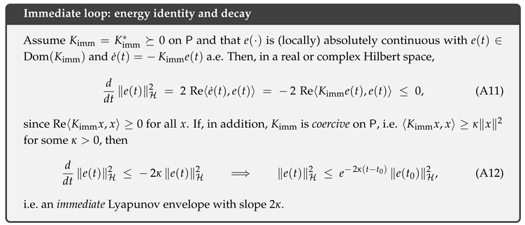
Appendix B.5. Why Interchangeability Matters.

Interchangeability (A9) ensures that the target $\mathcal{I}s$ and the response p are two representations of the same calibrated object in the same geometry. Consequently:

• The residual $R={\parallel p-\mathcal{I}s\parallel }^2$ is exactly the squared energy of e (A10); there is no hidden coupling to other “gauges’’ or spaces.
• A local (or diagonal) $K_{\mathrm{imm}}$ reduces epointwise/modewise, because p and $\mathcal{I}s$ are co-located in $\mathcal{H}$; the loop never needs to “translate’’ between spaces to know which way to push.
• Orthogonal projection identities in $\mathcal{H}$ give the one-line DPI for any admissible processing between steps, complementing the continuous-time decay (A12) [8].

Appendix B.6. Two Canonical Realizations (Educative Sketches).

• Operator–algebraic (GNS) setting.
  Work in $\mathcal{H}=L^2(\mathcal{M},\omega )$ for a faithful state $\omega$. Take $J^{(+)}$ as the $\omega$-preserving conditional expectation and $\mathcal{I}$ the inclusion; then $\mathcal{I}{J}^{(+)}={\mathrm{id}}_{\mathsf{P}}$, $J^{(+)}\mathcal{I}=P_{\mathsf{S}}$ [7,14,34,35]. Choose $K_{\mathrm{imm}}$ as the positive part of a symmetric Dirichlet form (e.g. the modular/carré-du-champ generator). The energy identity (A11) is the standard Dirichlet dissipation; coercivity gives (A12).
• PDE (gradient–channel) setting.
  Let $\mathcal{H}=L^2(\Omega ;{\mathbb{R}}^m)$, $e:=p-\mathcal{I}s$, and $\langle K_{\mathrm{imm}}e,e\rangle ={\int }_{\Omega }\langle B\left(x\right)\mathcal{L}e,\mathcal{L}e\rangle dx$, with $B\left(x\right)⪰\beta I$ and $\mathcal{L}$ local (e.g. ∇). Then $\dot{e}=-K_{\mathrm{imm}}e\Rightarrow {\displaystyle \frac{d}{dt}}{\parallel e\parallel }^2=-2\int \langle B\mathcal{L}e,\mathcal{L}e\rangle \le -2\beta {\parallel \mathcal{L}e\parallel }^2$, and a Poincaré/Helmholtz inequality yields (A12) with $\kappa =\beta {\lambda }_1$.

Appendix B.7. Summary.

Interchangeability places blueprint and response in the same Hilbert geometry, so the residual is a plain squared norm. If, in that geometry, the generator $K_{\mathrm{imm}}$ is local (or diagonal) and positive (coercive), then each coordinate/mode of e obeys an immediate one–dimensional decay, and the total energy follows by Pythagoras/Parseval. The slow loop ${\int }_0^{t}M(·)e$ encodes delayed, nonlocal corrections; causality throttles that relay across horizons, leaving the immediate loop to enforce the exterior Lyapunov envelope.

Appendix B.8. Propagation Identities and Lyapunov Envelopes

In the DSFL picture, once statistics and physics are co-located in the same Hilbert geometry, the propagation of the calibrated mismatch $e:=p-\mathcal{I}s$ is most naturally controlled by energy identities and comparison estimates. At this level of generality we do not assume a specific micromodel; we only require a sector–provided evolution law whose instantaneous (local) part is accretive and whose retarded (nonlocal) part is causal and positive. The key outcome is a Lyapunov envelope for the single observable $\mathcal{R}\left(t\right)={\parallel e\left(t\right)\parallel }_{\mathcal{H}}^2$: a differential inequality of the form $\dot{\mathcal{R}}\le -2(\kappa -\epsilon )\mathcal{R}$ implies exponential decay with a rate set by a coercivity margin $\kappa$ (the immediate loop’s gap) up to lower–order leakage $\epsilon$. The next paragraphs record the sector–specific residual identity that yields this envelope and the resulting semilog “straight–line’’ decay for $\mathcal{R}$.

Appendix B.8.1. Residual Identity (Sector–Specific).

When the sector supplies a differential identity for $e:=p-\mathcal{I}s$,

$${\displaystyle \frac{\mathrm{d}}{\mathrm{d}t}}{\parallel e\left(t\right)\parallel }_{\mathcal{H}}^2=-2{\langle Ke,e\rangle }_{\mathcal{H}}+2{\langle e,g\rangle }_{\mathcal{H}},$$

(A13)

with $K=K^{*}⪰0$ and ${|\langle e,g\rangle }_{\mathcal{H}}{|\le \epsilon \parallel e\parallel }_{\mathcal{H}}^2$, any calibrated gap/coercivity

$${\langle Ke,e\rangle }_{\mathcal{H}}\ge \kappa {\parallel e\parallel }_{\mathcal{H}}^2$$

yields a Lyapunov envelope:

$$\dot{\mathcal{R}}\left(t\right)\le -2(\kappa -\epsilon )\mathcal{R}\left(t\right)⟹\mathcal{R}\left(t\right)\le e^{-\alpha t}\mathcal{R}\left(0\right),\alpha :=2(\kappa -\epsilon )>0.$$

(A14)

Thus $log\mathcal{R}$ decays linearly with slope $-\alpha$ (semi–log straight line). The rate $\alpha$ is the sector’s single dial (gap minus lower–order leakage).

Appendix B.8.2. Operational Arrow.

The accumulated reduction

$$S_R\left(t\right):=-log{\displaystyle \frac{\mathcal{R}\left(t\right)}{\mathcal{R}\left(0\right)}}={\int }_0^t\alpha \left(\tau \right)\mathrm{d}\tau$$

(A15)

is monotone, quantifying “how much calibrated mismatch was removed’’ independent of clock parametrization.

Appendix B.9. Minimal Usage (Practitioner Checklist)

• Pick the geometry: choose $\mathcal{H}$ so both channels embed naturally.
• Calibrate: construct $(\mathcal{I},J^{(+)})$ with (A3).
• Gate admissibility: verify (A5) for your updates (and budget preservation if using (A7)).
• Read off a rate: identify $(\kappa ,\epsilon )$ in (A13) to obtain $\alpha =2(\kappa -\epsilon )$ and the envelope (A14).
• Report R and $S_R$: track $\mathcal{R}$ and its semi–log slope; compare design choices by $S_R$.

Appendix B.10. Remarks (Existence, Uniqueness, Robustness)

• Nonuniqueness of $(\mathcal{I},J^{(+)})$. Many calibrations may realize (A3); results that rely only on (A6) are invariant under switching to any other $({\mathcal{I}}^{\prime },J^{(+)}\prime )$ with the same image $\mathrm{Im}\mathcal{I}$.
• Robustness of DPI. Any $\mathsf{\Phi }$ with $\parallel \mathsf{\Phi }\parallel \le 1$ and intertwining survives composition and limits; DPI extends to piecewise–constant and time–varying admissible flows.
• Local vs nonlocal dynamics. The propagation identity (A13) can represent local dissipation ($K_{\ell }$) plus causal memory kernels (Volterra terms); only the coercivity margin matters for (A14).

References

- Hawking, S.W.; Ellis, G.F.R. The Large Scale Structure of Space–Time; Cambridge University Press: Cambridge, 1973.
- Wald, R.M. General Relativity; University of Chicago Press: Chicago, 1984.
- Giddings, S.B. Nonviolent information transfer from black holes: a field theory parametrization. Physical Review D 2013, 88, 064023. [Google Scholar] [CrossRef]
- Harlow, D. Jerusalem Lectures on Black Holes and Quantum Information. Reviews of Modern Physics 2016, 88, 015002. [Google Scholar] [CrossRef]
- Penington, G. Entanglement Wedge Reconstruction and the Information Paradox. Journal of High Energy Physics 2020, 2020, 002. [Google Scholar] [CrossRef]
- Almheiri, A.; Hartman, T.; Maldacena, J.; Shaghoulian, E.; Tajdini, A. The Island Formula for the Entanglement Entropy. Journal of High Energy Physics 2020, 2020, 013. [Google Scholar] [CrossRef]
- Ohya, M.; Petz, D. Quantum Entropy and Its Use; Texts and Monographs in Physics, Springer: Berlin, 1993.
- Bauschke, H.H.; Combettes, P.L. Convex Analysis and Monotone Operator Theory in Hilbert Spaces, 2 ed.; CMS Books in Mathematics, Springer: Cham, 2017. [CrossRef]
- Gripenberg, G.; Londen, S.O.; Staffans, O. Volterra Integral and Functional Equations; Cambridge University Press: Cambridge, 1990.
- Dafermos, M.; Rodnianski, I. The red-shift effect and radiation decay on black hole spacetimes. Communications on Pure and Applied Mathematics 2009, 62, 859–919. [Google Scholar] [CrossRef]
- Berti, E.; Cardoso, V.; Starinets, A.O. Quasinormal modes of black holes and black branes. Classical and Quantum Gravity 2009, 26, 163001. [Google Scholar] [CrossRef]
- Breuer, H.P.; Petruccione, F. The Theory of Open Quantum Systems; Oxford University Press, 2002.
- Petz, D. Monotonicity of Quantum Relative Entropy. Reviews in Mathematical Physics 2003, 15, 79–91. [Google Scholar] [CrossRef]
- Takesaki, M. Theory of Operator Algebras II; Vol. 125, Encyclopaedia of Mathematical Sciences, Springer: Berlin, 2003.
- Dafermos, M.; Rodnianski, I. A new physical-space approach to decay for the wave equation, 2010. Preprint; see also arXiv:0910.4957.
- Dafermos, M.; Rodnianski, I. The red-shift effect and radiation decay on black hole spacetimes. Communications on Pure and Applied Mathematics 2010, 62, 859–919. [Google Scholar] [CrossRef]
- Stinespring, W.F. Positive Functions on C*-Algebras. Proceedings of the American Mathematical Society 1955, 6, 211–216. [Google Scholar]
- Kraus, K. General state changes in quantum theory. Annals of Physics 1971, 64, 311–335. [Google Scholar] [CrossRef]
- Kadison, R.V. A generalized Schwarz inequality and algebraic invariants for operator algebras. Annals of Mathematics 1952, 56, 494–503. [Google Scholar] [CrossRef]
- Bhatia, R. Matrix Analysis; Vol. 169, Graduate Texts in Mathematics, Springer: New York, 1997. [CrossRef]
- Unruh, W.G. Notes on black-hole evaporation. Physical Review D 1976, 14, 870–892. [Google Scholar] [CrossRef]
- Lindblad, G. Completely Positive Maps and Entropy Inequalities. Communications in Mathematical Physics 1975, 40, 147–151. [Google Scholar] [CrossRef]
- Uhlmann, A. Relative entropy and the Wigner–Yanase–Dyson–Lieb concavity in an interpolation theory. Communications in Mathematical Physics 1977, 54, 21–32. [Google Scholar] [CrossRef]
- Cover, T.M.; Thomas, J.A. Elements of Information Theory, 2 ed.; Wiley Series in Telecommunications and Signal Processing, Wiley: Hoboken, NJ, 2006. [CrossRef]
- Hawking, S.W.; King, A.R.; McCarthy, P.J. A New Topology for Curved Space-time which Incorporates the Causal, Differential, and Conformal Structures. Journal of Mathematical Physics 1976, 17, 174–181. [Google Scholar] [CrossRef]
- Hawking, S.W. Breakdown of Predictability in Gravitational Collapse. Physical Review D 1976, 14, 2460. [Google Scholar] [CrossRef]
- Wald, R.M. Quantum Field Theory in Curved Spacetime and Black Hole Thermodynamics; University of Chicago Press, 1994.
- Page, D.N. Average Entropy of a Subsystem. Physical Review Letters 1993, 71, 1291–1294. [Google Scholar] [CrossRef]
- Page, D.; Wootters, W. Evolution without evolution Dynamics described by stationary observables. Physical Review D 1983, 27, 2885. [Google Scholar] [CrossRef]
- Almheiri, A.; Marolf, D.; Polchinski, J.; Sully, J. Black Holes: Complementarity or Firewalls? Journal of High Energy Physics 2013, 2013, 062. [Google Scholar] [CrossRef]
- Mathur, S.D. The Information Paradox: A Pedagogical Introduction. Classical and Quantum Gravity 2009, arXiv:hep-th/0909.1038]26, 224001. [Google Scholar] [CrossRef]
- Susskind, L.; Thorlacius, L.; Uglum, J. The Stretched Horizon and Black Hole Complementarity. Physical Review D 1993, 48, 3743–3761. [Google Scholar] [CrossRef]
- ’t Hooft, G. Dimensional reduction in quantum gravity. arXiv preprint 1993, [gr-qc/9310026].
- Takesaki, M. Conditional Expectations in von Neumann Algebras. Journal of Functional Analysis 1972, 9, 306–321. [Google Scholar] [CrossRef]
- Tomiyama, J. On the Projection of Norm One in W*-Algebras. Proceedings of the Japan Academy 1957, 33, 608–612. [Google Scholar] [CrossRef]
- Bauerschmidt, R.; Brydges, D.C.; Slade, G. Introduction to a Renormalisation Group Method; Vol. 2242, Lecture Notes in Mathematics, Springer, 2021.
- Nachtergaele, B.; Sims, R. Lieb–Robinson bounds and the exponential clustering theorem. Communications in Mathematical Physics 2006, 265, 119–130. [Google Scholar] [CrossRef]
Disclaimer/Publisher’s Note: The statements, opinions and data contained in all publications are solely those of the individual author(s) and contributor(s) and not of MDPI and/or the editor(s). MDPI and/or the editor(s) disclaim responsibility for any injury to people or property resulting from any ideas, methods, instructions or products referred to in the content. |
© 2025 by the authors. Licensee MDPI, Basel, Switzerland. This article is an open access article distributed under the terms and conditions of the Creative Commons Attribution (CC BY) license (http://creativecommons.org/licenses/by/4.0/).
Copyright: This open access article is published under a Creative Commons CC BY 4.0 license, which permit the free download, distribution, and reuse, provided that the author and preprint are cited in any reuse.