Proving an Arrow of Time Under Universal Time: A DSFL Framework for Black-Hole Evaporation

1. Introduction

Time in relativity is relational and frame–dependent: proper time follows worldlines, and coordinate time can be reparametrized without physical effect [1,2]. Yet many irreversible phenomena exhibit a robust arrow of time that is not tied to a particular clock choice. This paper develops a clock–neutral, operational arrow based on a single quadratic observable defined in one comparison geometry. The central claim is that, once statistics (what is prescribed) and physics (what happens) are co–located in a common Hilbert space, a minimal notion of “time flow’’ is simply the monotone contraction of a calibrated residual of sameness. This arrow is intrinsic (invariant under time reparametrization), causal (throttled by domain–of–dependence), and testable (Lyapunov envelopes, data–processing checks). General relativity supplies the background causal structure; the DSFL framework supplies the universal yardstick and the monotonicity theorems.

1.1. A Universal Yardstick for Time’s Arrow

We embed the statistical blueprint (what the model “asks for”) and the physical response (what the system “does”) into the same Hilbert geometry $(\mathcal{H},\langle ·,·\rangle )$. The calibration pair

$$\mathcal{I}:\mathsf{S}\to \mathsf{P},J^{(+)}:\mathsf{P}\to \mathsf{S},\mathcal{I}{J}^{(+)}={\mathrm{id}}_{\mathsf{P}},J^{(+)}\mathcal{I}=P_{\mathsf{S}},$$

(1)

aligns units, gauges, and types between channels. The single observable we track is the calibrated residual of sameness

$$R(s,p):=\parallel p-\mathcal{I}s{\parallel }_{\mathcal{H}}^2,$$

(2)

which vanishes precisely when the response pis the calibrated image $\mathcal{I}s$. Operationally, “time flows’’ if Rdecreases. Because R is a norm in a fixed geometry, it is invariant under any admissible change of coordinates or polarization that preserves $\mathrm{Im}\mathcal{I}$; and because our inequalities are homogeneous in time, they are invariant under any strictly increasing reparametrization of the time parameter (“clock–neutrality”).

1.2. Two Structural Principles (Arrow and Causality)

(i) Admissibility ⇒ data processing A physically allowed step $(\tilde{\Phi },\Phi )$ must respect calibration and be nonexpansive in the comparison norm:

$$\Phi \mathcal{I}=\mathcal{I}\tilde{\Phi },{\parallel \Phi \parallel }_{\mathcal{H}\to \mathcal{H}}\le 1.$$

(3)

Then the Hilbert–space data–processing inequality (DPI) holds in one line,

$$R(\tilde{\Phi }s,\Phi p)=\parallel \Phi \left(p-\mathcal{I}s\right){\parallel }_{\mathcal{H}}^2\le {\parallel p-\mathcal{I}s\parallel }_{\mathcal{H}}^2=R(s,p),$$

(4)

so no admissible coarse–graining or channel composition can increase R [3,4]. This monotonicity supplies an intrinsic arrow independent of clock choice.

(ii) Dual–scale feedback ⇒ Lyapunov envelope & causal ceiling When dynamics are present, the calibrated mismatch $e:=p-\mathcal{I}s$ evolves by a universal two–loop law,

$$\dot{e}\left(t\right)=-K_{\mathrm{imm}}e\left(t\right)-{\int }_0^{t}M(t-\tau )e\left(\tau \right)d\tau +r\left(t\right),$$

(5)

with an immediate (local) dissipative loop $K_{\mathrm{imm}}⪰0$ and a slow (nonlocal) causal relay $M\in L^1\left([0,\infty )\right)$[5]. Causal boundaries (e.g. event horizons) throttle the slow loop: the retarded kernel has null/timelike support and cannot relay calibrated content across a causally sealed boundary [1,2]. The exterior then closes to ${\dot{e}}_U=-K_{\mathrm{imm}}{e}_U+r_U$, so the exterior residual admits a Lyapunov (ringdown) envelope with slope set by the least–damped mode of the immediate loop (red–shift/quasinormal modes) [6,7].

1.3. How DSFL Differs from (and Complements) Relativity

Einstein’s relativity fixes how clocks relate across frames (proper time, gravitational red–shift) and supplies the causal scaffolding of spacetime (light cones, horizons) [1,2,8]. DSFL does not change these facts. It adds a complementary layer: an observer– and clock–neutral notion of temporal direction defined by a single, sector–neutral observable R in one comparison geometry, together with a canonical reparametrization that makes the decay of R universal. The key separations are:

• Universal direction (DSFL) vs. symmetric equations (GR) GR’s field equations are time–reversal symmetric on generic Cauchy data. DSFL installs a kinematic gate (admissibility: intertwining + nonexpansiveness) that yields a Hilbert–space DPI: $R(\tilde{\Phi }s,\Phi p)\le R(s,p)$. Hence the calibrated residual cannot increase under any physically allowed step—an intrinsic arrow independent of coordinates or foliation. (DPI: §Section 2, §Section 3)
• From GR rates to a DSFL clock GR supplies what damps (exterior gaps from red–shift/QNMs) and where signals reach (domain of dependence). DSFL turns these inputs into a Lyapunov envelope and an intrinsic clock: with $\lambda \left(t\right)=\kappa \left(t\right)-\epsilon \left(t\right)\ge 0$ one has $\dot{R}\le -2\lambda R$ and, in DSFL time $d\widehat{\tau }=2\lambda \left(t\right)dt$, the unit–slope law $dR/d\widehat{\tau }\le -R$. (Envelope/clock: Thm. 2, Prop. 2, Thm. 3)
• Causality roles: GR constrains support; DSFL enforces no–relay GR’s cones/horizons fix the causal ceiling; DSFL encodes it as vanishing interior→exterior relay in the slow loop (retarded kernel). The exterior closes to the immediate loop and inherits the ringdown envelope; no “revival’’ from behind the horizon is allowed. (No–relay: Prop. 3)
• Universality under recalibration/sector changes Proper time depends on worldlines; DSFL’s arrow and clock depend on the comparison geometry. Under any isometry $U:\mathcal{H}\to \mathcal{H}$ with pushforward of $(\mathcal{I},K_{\mathrm{imm}},M)$, one has invariance of R, $\lambda$, and $d\widehat{\tau }$. Thus the decay law and unit–slope timeline are calibration/sector invariant. (Lemma 2, Thm. 4)
• Distinct, falsifiable testables DSFL predictions are phrased as: (i) no growth of the calibrated $L^2$ residual under any admissible processing (DPI checks); (ii) semi–log straight–line ringdown slopes determined by exterior gaps (rate extraction); (iii) zero fitted interior→exterior memory blocks after horizon formation (causal ceiling); (iv) discrete ticks that sum to the continuum clock via $\Delta \widehat{\tau }=-log(R_{k+1}/R_k)$ (tick composition). These signatures are invariant under time reparametrization and recalibration and are orthogonal to standard frame-dependent clock tests. (Sec. Section 1.6; Thm./Prop. references above)

Summary GR tells us where influence can flow and how fast exteriors damp; DSFL tells us what necessarily decreases (the calibrated residual) and provides a universal, clock–neutral time in which every lawful evolution decays with unit slope. Together they yield a precise, testable arrow of time without altering relativity.

1.4. Black Holes as a Proving Ground (Without Changing the Clocks)

Black–hole exteriors provide a clean laboratory for the DSFL arrow. A single “Hawking tick”—pair creation near the horizon followed by tracing the interior partner—is a completely positive, Heisenberg–unital step (Stinespring/Kraus) and therefore $L^2$–nonexpansive [3,9]. Modeled as $({\tilde{\Phi }}_{\mathrm{Hawk}},{\Phi }_{\mathrm{Hawk}})$, it satisfies (4) stepwise:

$$R({\tilde{\Phi }}_{\mathrm{Hawk}}s,{\Phi }_{\mathrm{Hawk}}p)\le R(s,p).$$

(6)

Local KMS thermality of exterior marginals is compatible with this DPI; microstate dependence can reside in correlations (early/late radiation or island wedges) without forcing any increase of exterior R[10,11,12,13]. Thus the DSFL arrow of time—monotone contraction of R with a ringdown envelope—is realized in a strictly clock–neutral way that complements, rather than competes with, Einsteinian relativity.

1.5. What This Buys

Tracking the wrong observable (marginal entropy of a subsystem) obscures the arrow; tracking the right one (a calibrated $L^2$ residual) exposes it and makes it testable. In this paper we:

• formalize the DSFL kinematics (interchangeability, R, admissibility) and prove global/exterior DPIs for R;
• derive a causal “no–relay” barrier at horizons and an exterior Lyapunov (ringdown) envelope;
• model Hawking ticks as admissible channels, reconciling locally thermal flux with stepwise contraction of R;
• introduce a one–budget convention (no duplication of statistical content) that explains how correlations grow without inflating any exterior residual; and
• spell out falsifiable diagnostics: projection/DPI checks, semi–log ringdown slopes, relay toggles, and radiation correlation structure.

Throughout, the mathematics is elementary (orthogonal projections and nonexpansive maps in $\mathcal{H}$), the physics enters through causality and exterior decay, and the arrow of time appears as a theorem about a single, operational observable—independent of which clock one uses to label the steps.

1.6. Roadmap

subsec:dsfl-primer-conclusion gives a two–page primer on the comparison geometry, interchangeability, the residual $\mathcal{R}$, and admissibility. sec:bh-info-paradox then states the trilemma and sets the DSFL kinematics, proving a global/exterior Hilbertian DPI and deriving the dual–scale (fast/slow) feedback law with a causal ceiling at the horizon, which yields an exterior Lyapunov (ringdown) envelope from red–shift/QNM coercivity. Next, in Hawking channel as an admissible map we model each “tick’’ as a Stinespring/Kraus CP–unital step and show stepwise $L^2$-nonexpansiveness (with supporting operator–algebra citations), reconcile local KMS thermality with monotone exterior R, and connect to Page/island purification via correlations. The subsection Form of the paradox in DSFL variables restates what is actually constrained (the calibrated misfit R), followed by Resolution template giving stand-alone statements with proofs/sketches (no-inflation, causal throttling, exterior envelope, Hawking admissibility, global DPI). We then provide What can be tested (subsec:falsifiability-dsfl)—a falsifiability/diagnostics suite—and a geometric add-on (subspace–angle contraction) for calibration quality and per-step guarantees. Appendices include notation and a Generic Two–Channel Application Template for porting the scheme to other sectors. Throughout, the mathematics is deliberately elementary (orthogonal projections, nonexpansive maps in $\mathcal{H}$, Stinespring/Kraus), while the physics enters through causality and established exterior decay mechanisms.

1.7. What Has Been Done on the Arrow of Time (Concise Literature Map)

1.7.1. Statistical Origins and Classical Irreversibility

The modern “arrow’’ begins with Boltzmann’s H–theorem and kinetic programme [14,15], immediately challenged by Loschmidt’s reversibility and Zermelo’s recurrence objections [16,17]. Gibbs’ ensembles and coarse–graining reframed typicality and macrostates [18], while Lanford’s theorem clarified the Boltzmann–Grad limit for short times [19]. Eddington popularized the “arrow of time’’ as macroscopic irreversibility [20,21]; Ehrenfest–type models illustrated approach to equilibrium [22]. Linear nonequilibrium thermodynamics (Onsager, Kubo) connected entropy production to response [23,24,25].

1.7.2. Quantum Open Systems, Entropy Production, and Data Processing

In quantum dynamics, completely positive semigroups (GKS–Lindblad) supply the canonical irreversible evolutions [26,27]. Spohn’s inequality and Davies theory put entropy production and detailed balance on operator footing [28,29]. Monotonicity of quantum relative entropy (data–processing) was established by Lindblad, Uhlmann, Lieb–Ruskai, and Petz [30,31,32,33]; modular theory and conditional expectations yield nonexpansive projections in $L^2$ [3,34,35,36]. Stinespring/Kraus dilations and Schatten–2 contractivity underpin stepwise coarse–grained arrows [37,38,39]. Classical information DPI and fluctuation theorems give complementary statements [40,41,42,43,44,45,46].

1.7.3. Locality and Causal Speed Limits

Lieb–Robinson bounds and their refinements quantify finite–speed propagation in lattice and continuum systems—operator–level causal cones for many–body dynamics [47,48,49,50]. These provide rigorous “no–relay’’ constraints for retarded kernels.

1.7.4. GR, Horizons, and Gravitational Arrows

Einstein’s field equations supply proper time and causal cones but are time–reversal invariant in generic settings [1,8,51]. Irreversibility enters through global/causal structures: Hawking’s area theorem, Bekenstein–Hawking entropy, and semiclassical radiation [52,53,54,55]. Exterior decay and red–shift/Price laws establish quantitative relaxation (ringdown) [6,56,57], and QNM spectra organize late–time behaviour [7]. Cosmological “arrows’’ include Weyl–curvature ideas [58] and modern expositions [59].

1.7.5. Black–Hole Information, Page Curve, and Islands

Unitary evaporation constraints (Page curve) and firewall/complementarity debates [10,11,60,61,62,63,64] were reframed by replica–wormhole/island computations that reassign entanglement wedges while keeping semiclassical exteriors [12,13].

1.7.6. Why These Strands Matter for “Time’’ in DSFL

(i) Monotonicities (quantum DPI, Spohn/Lindblad) justify kinematic arrows under coarse–graining [3,30,31,33]. (ii) Locality (Lieb–Robinson, domain–of–dependence) supplies causal ceilings—no instantaneous relay [1,2,47,48]. (iii) Exterior decay (red–shift/Price/QNMs) turns the arrow quantitative (a slope) [6,7,57]. (iv) Islands/Page locate unitarity in correlations, compatible with local arrows for calibrated R [11,12,13]. (v) Einsteinian GR contributes the metric and cones [8,51]; DSFL contributes a single, calibrated Lyapunov functional and a clock–neutral time in which every admissible evolution decays with unit slope.

1.8. Contributions (What Is Proved in This Paper)

1.8.1. One Observable and Kinematics

• Global/exterior Hilbertian DPI for the calibrated residual${\displaystyle R(s,p)={\parallel p-\mathcal{I}s\parallel }_{\mathcal{H}}^2}$. For every admissible step $(\tilde{\Phi },\Phi )$ (intertwining $\Phi \mathcal{I}=\mathcal{I}\tilde{\Phi }$, nonexpansive ${\parallel \Phi \parallel }_{\mathcal{H}\to \mathcal{H}}\le 1$),

  $$R(\tilde{\Phi }s,\Phi p)=\parallel \Phi (p-\mathcal{I}s){\parallel }_{\mathcal{H}}^2\le {\parallel p-\mathcal{I}s\parallel }_{\mathcal{H}}^2=R(s,p),$$

  (7)

  so no physically allowed coarse–graining increases the calibrated mismatch. (Kinematic arrow; clock–neutral.) (Thm/Prop: DPI statements; §Section 2, §Section 3)

1.8.2. Dynamics and Rate (Dual–Scale Feedback)

• Exterior Lyapunov (ringdown) envelope For the dual–scale Volterra law $\dot{e}=-K_{\mathrm{imm}}e-{\int }_0^{t}M(t-\tau )e\left(\tau \right)d\tau +r$ with $K_{\mathrm{imm}}=K_{\mathrm{imm}}^{*}⪰0$, $\langle K_{\mathrm{imm}}x,x\rangle \ge \kappa \left(t\right){\parallel x\parallel }^2$, $M⪰0$ (retarded), and $\left|\langle r,x\rangle \right|\le {\epsilon \left(t\right)\parallel x\parallel }^2$, the exterior residual obeys

  $${\dot{R}}_{\mathrm{out}}\left(t\right)\le -2\lambda \left(t\right)R_{\mathrm{out}}\left(t\right),\lambda \left(t\right):=\kappa \left(t\right)-\epsilon \left(t\right)\ge 0,$$

  (8)

  hence $R_{\mathrm{out}}\left(t\right)\le e^{-2\int \lambda }{R}_{\mathrm{out}}\left(t_0\right)$. (Quantitative arrow; rate = least–damped exterior mode.) (Thm.2, Corollary “QNM/rate”, §Section 3)
• Causal no–relay across horizons If M has null/timelike support, then after horizon formation ${\int }_0^t{M}_{U\leftarrow \mathcal{H}}(t-\tau )e\left(\tau \right)d\tau \equiv 0$. The exterior closes to the immediate loop and inherits the envelope. (Prop.3, §Section 3)

1.8.3. Clock–Neutral Time and Universality

• Intrinsic DSFL time and unit–slope law With $d\widehat{\tau }=2\lambda \left(t\right)dt$, ${\displaystyle \frac{dR}{d\widehat{\tau }}}\le -R$ and $R\left(\widehat{\tau }\right)\le e^{-(\widehat{\tau }-{\widehat{\tau }}_0)}R\left({\widehat{\tau }}_0\right)$. The statement is invariant under any strictly increasing reparametrization and unique up to an affine change. (Prop.2, Thm.3, §Section 3.9)
• Universality across calibrations/sectors If $U:\mathcal{H}\to \mathcal{H}$ is an isometry and we push forward $(\mathcal{I},K_{\mathrm{imm}},M)$, then R, $\lambda$, and $d\widehat{\tau }$ are unchanged. (Invariance of the arrow and the clock.) (Lemma2, Thm.4)

1.8.4. Discrete Ticks and Hawking Channel

• Hawking tick admissibility & stepwise contraction A single emission step (Stinespring/Kraus dilation + interior trace) is Heisenberg–unital CP ⇒$L^2$–nonexpansive; hence $R_{k+1}\le R_k$ per tick. Discrete DSFL time $\Delta {\widehat{\tau }}_k:=-log(R_{k+1}/R_k)\ge 0$ composes multiplicatively to the continuum envelope. (Cor.6, Prop.4, §Section 3)

1.8.5. One–Budget Law and Entanglement Mechanism

• Budget conservation and no duplication With $s=w{s}_0$, $\int w=1$, admissible statistical updates are Markov (mass–preserving): budget can be redistributed and correlated but not cloned (no $w\to w\oplus w$, no $e\to (e,e)$). (Lemma1, Cor.1, Prop.11, §Section 6.9)
• No perfect broadcasting of incompatibles If two noncommuting presentations are to be preserved simultaneously with DPI for all inputs, they must commute; otherwise some R inflates. (Budget–language restatement of no–broadcasting.) (Prop.12)
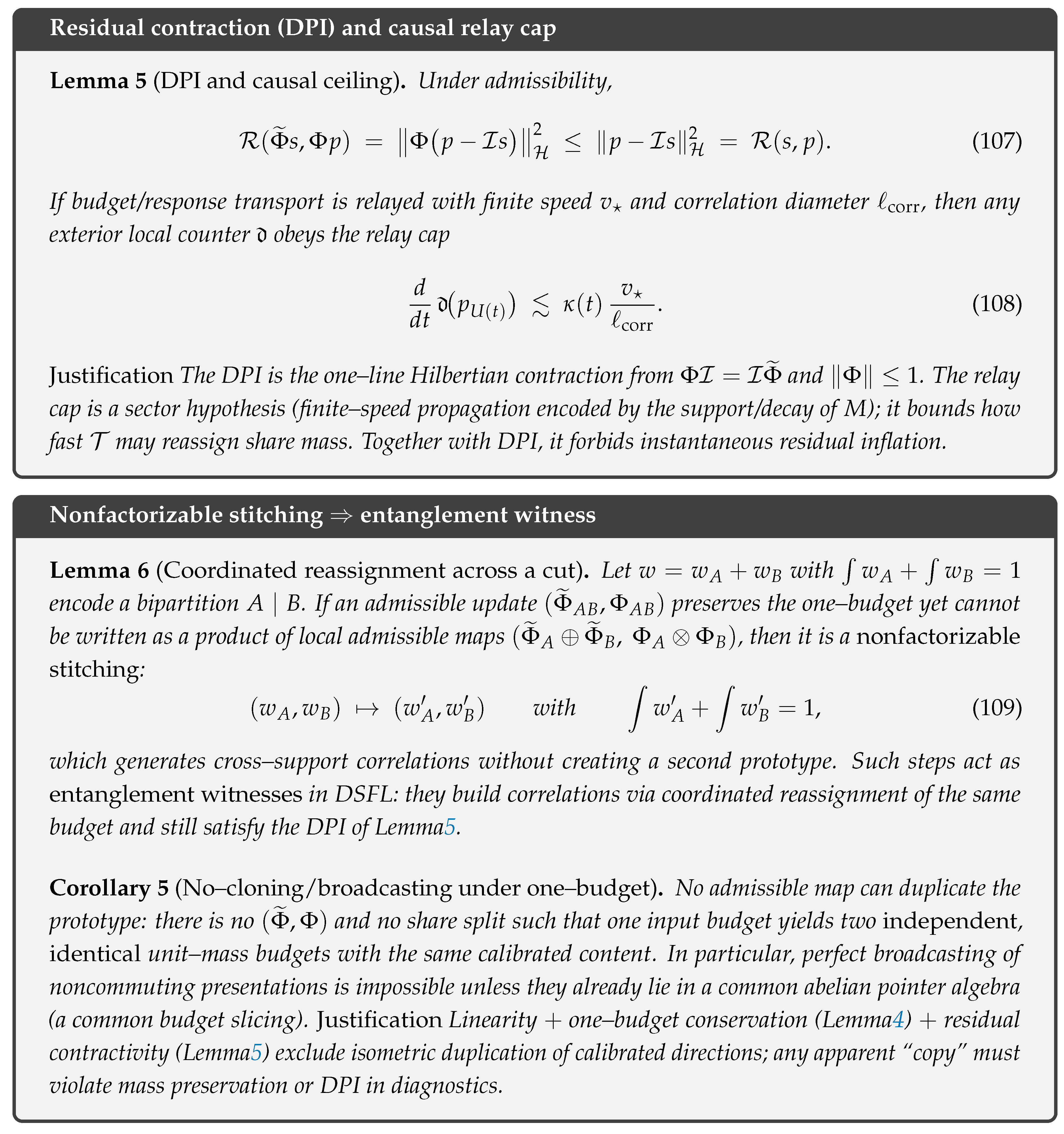
• Entanglement as coordinated reassignment Nonfactorizable “stitching’’ across a cut increases correlations while keeping local/exterior R nonincreasing; this is the unitary mechanism compatible with the local arrow. (§Section 6.9.12, Prop.13)

1.8.6. Geometry–Set Progress Per Step

• Subspace–angle tick bound If a block implements (exact or approximate) orthogonal projection onto $V=\overline{\mathrm{ran}\mathcal{I}}$, then

  $$R_{\mathrm{after}}\le {sin}^2{\theta }_F{R}_{\mathrm{before}},\Delta \widehat{\tau }:=-log\left({\displaystyle \frac{R_{\mathrm{after}}}{R_{\mathrm{before}}}}\right)\ge -log\left({sin}^2{\theta }_F\right).$$

  (9)
  This is a clock–neutral, dynamics–free lower bound on the per–step DSFL time advance, set purely by the Friedrichs angle ${\theta }_F$ between $U=\mathsf{P}$ and $V=\overline{\mathrm{ran}\mathcal{I}}$. (Prop.1, §Geometric context)

1.8.7. Separation from GR (What DSFL Adds)

• No GR–only local Lyapunov Time–reversal symmetric Einstein–matter Cauchy problems admit no strictly monotone, diffeo–covariant local scalar for generic data; DSFL provides one by calibration and admissibility. (Prop.15, §Section 10.4)
• Using GR to get a DSFL clock GR gives cones and exterior gaps (red–shift/QNM), while DSFL turns them into a Lyapunov arrow and an intrinsic, unit–slope time. (Thm.13, Thm.14)

1.8.8. What We Do Not Claim

• We do not derive von Neumann–entropy Page curves; we prove contraction for $L^2$–residuals and explain how purification lives in correlations (islands/early–late radiation) without increasing any exterior R.
• We do not modify GR or semiclassical QFT; all physics enters via causal support and established exterior decay.

2. DSFL in Two Pages (Self-Contained Primer for New Readers)

Discussions of “information loss” or “purification” often compare quantities that live in different mathematical spaces (fields, states, coarse-grained observables). To reason cleanly about what can or cannot increase under physically allowed operations, we place both sides of the description—statistics and physics— into one Hilbert geometry and measure a single, objective gap. The DSFL claim is deliberately modest: once statistics and physics are co-located in a common geometry, the one observable that semiclassics can provably control is a calibrated $L^2$-residual. Everything else (e.g. purification) is delegated to correlations rather than to local marginals.

2.1. Common Comparison Geometry

Fix a (real or complex) Hilbert space $(\mathcal{H},\langle ·,·\rangle )$ with norm $\parallel x\parallel :=\sqrt{\langle x,x\rangle }$. We embed:

- a statistical blueprint channel $\mathsf{S}$ (what the model “asks” for), and - a physical response channel $\mathsf{P}\subset \mathcal{H}$ (what the system “does”)

in the same $\mathcal{H}$. This co-location makes comparisons well-typed, Euclidean, and orthogonalizable.

2.2. Interchangeability (Calibration) Maps

A calibration pair

$$\mathcal{I}:\mathsf{S}\to \mathsf{P},J^{(+)}:\mathsf{P}\to \mathsf{S}$$

(10)

is required to satisfy

$$\mathcal{I}{J}^{(+)}={\mathrm{id}}_{\mathsf{P}},J^{(+)}\mathcal{I}=P_{\mathsf{S}},$$

(11)

where $P_{\mathsf{S}}$ is the orthogonal projector onto the blueprint subspace $\mathsf{S}\subset \mathcal{H}$. Equation (11) encodes two-way coherence: pushing a physical response to the blueprint and back is the identity on the physical side; pulling a blueprint to the physical side and back projects to the canonical blueprint subspace. Intuitively, $(\mathcal{I},J^{(+)})$ is the calibrated meter that says when “model” and “device” are literally the same object in $\mathcal{H}$.

2.3. Residual of Sameness

With $(s,p)\in \mathsf{S}\times \mathsf{P}$ we track a single observable—the calibrated misfit

$$\mathcal{R}(s,p):=\parallel p-\mathcal{I}s{\parallel }_{\mathcal{H}}^2\ge 0,\mathcal{R}(s,p)=0⟺p=\mathcal{I}s\left(\mathrm{perfect}\mathrm{match}\right).$$

(12)

$\mathcal{R}$ is the “thermometer” for sameness: it vanishes iff the physical response is exactly the calibrated image of the blueprint. Because $\mathcal{R}$ is purely metric in $\mathcal{H}$, it is invariant under any isometry $U:\mathcal{H}\to \mathcal{H}$ with $U\left(\mathrm{Im}\mathcal{I}\right)=\mathrm{Im}\mathcal{I}$ (change of basis, polarization, or coordinates that preserve the calibrated image).

2.4. Admissible (Physically Allowed) Updates

An update $(\tilde{\Phi },\Phi )$—think “model step” on $\mathsf{S}$ and “physical step” on $\mathsf{P}$—is admissible if it satisfies

$$\Phi \mathcal{I}=\mathcal{I}\tilde{\Phi }{(\mathrm{intertwining}\mathrm{of}\mathrm{calibration})\mathrm{and}\parallel \Phi \parallel }_{\mathcal{H}\to \mathcal{H}}\le 1(\mathrm{nonexpansive}/\mathrm{contractive}\mathrm{in}\mathcal{H}).$$

(13)

The first identity says “do the model step and then calibrate’’ equals “calibrate and then do the physical step.’’ The second says the physical step cannot amplify distances in the comparison geometry. Both properties are stable under composition, so sequences and flows of admissible maps remain admissible. In particular, admissible steps are the discrete counterparts of the continuous immediate (local) loop and slow (causal, nonlocal) relay used later.

2.5. Data–processing inequality (DPI) and clock–neutral arrow

From (13) and (12):

$$\mathcal{R}(\tilde{\Phi }s,\Phi p)=\parallel \Phi (p-\mathcal{I}s){\parallel }_{\mathcal{H}}^2\le {\parallel p-\mathcal{I}s\parallel }_{\mathcal{H}}^2=\mathcal{R}(s,p).$$

(14)

Thus no admissible evolution can inflate the calibrated residual. This supplies an intrinsic arrow of time: the monotonicity of $\mathcal{R}$ is invariant under any strictly increasing reparametrization of the evolution parameter (i.e. it is “clock–neutral’’).

2.6. Data–processing inequality (DPI) in one line

From (13) and (12) we immediately get

$$\mathcal{R}(\tilde{\Phi }s,\Phi p)=\parallel \Phi \left(p-\mathcal{I}s\right){\parallel }_{\mathcal{H}}^2\le {\parallel p-\mathcal{I}s\parallel }_{\mathcal{H}}^2=\mathcal{R}(s,p).$$

(15)

Thus no admissible evolution can inflate the calibrated residual. This is the core monotonicity used throughout: it supplies an intrinsic arrow independent of coordinates, coarse–graining, or the choice of time parameter. In particular, the DPI is clock–neutral: it holds for any ordering of admissible steps and any strictly increasing reparametrization of the evolution parameter.

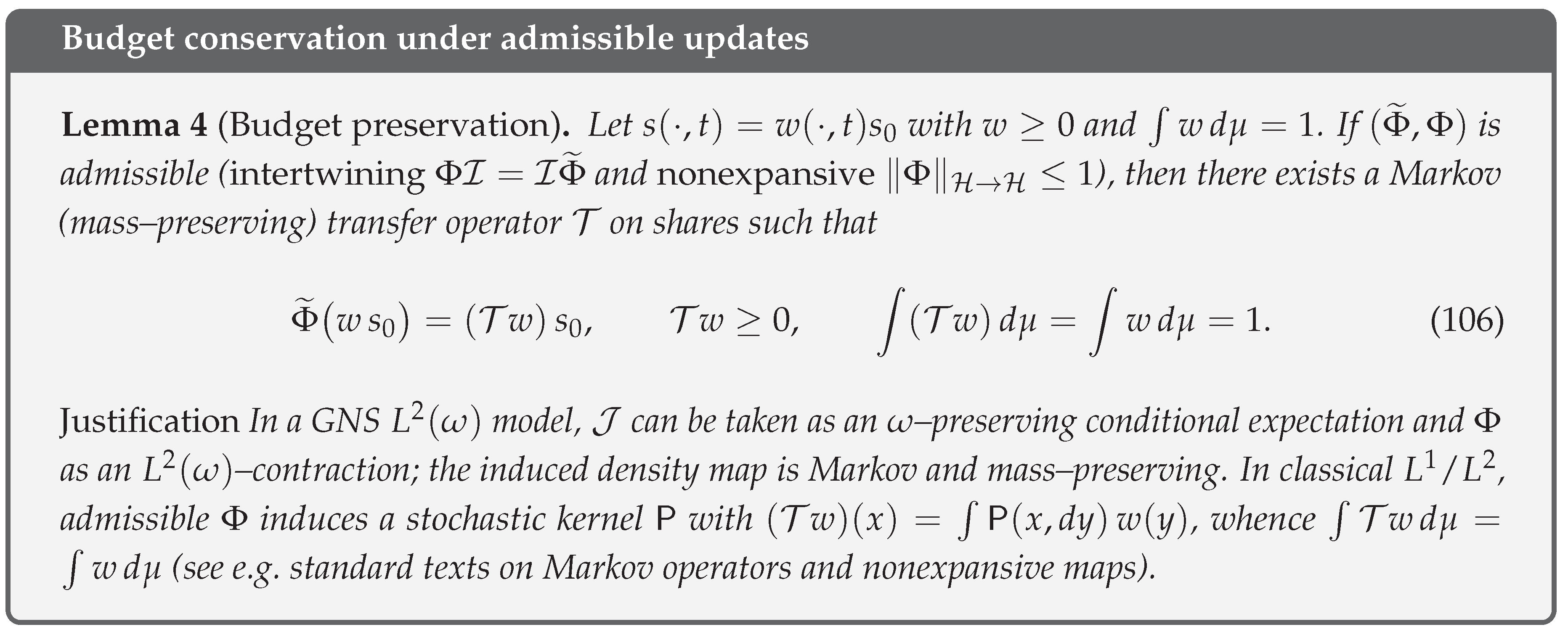
2.7. One–budget convention (no duplication of description)

To make “no cloning of description’’ precise, we represent the statistical content as a reweighting of a fixed prototype:

$$s(·,t)=w(·,t)s_0,w\ge 0,\int wd\mu =1.$$

(16)

Admissible updates may redistribute the share w (move blueprint weight around) but cannot create new statistical degrees of freedom. This “one stock of sDoF’’ rule prevents hidden double–counting: every apparent “split’’ is a partition of the same budget, not the birth of an additional prototype.

Lemma 1 

(Budget preservation as a Markov pushforward). Assume the one–budget ansatz $s(·,t)=w(·,t)s_0$ with $w\ge 0$ and $\int wd\mu =1$. If $(\tilde{\Phi },\Phi )$ is admissible and $\tilde{\Phi }$ acts locally on w through a linear positive operator $\mathcal{T}$ (i.e. $\tilde{\Phi }\left(w{s}_0\right)=\left(\mathcal{T}w\right)s_0$), then $\mathcal{T}$ is Markov:

$$\mathcal{T}w\ge 0,\int \left(\mathcal{T}w\right)d\mu =\int wd\mu =1.$$

(17)

Proof. 

Positivity follows from positivity of $\tilde{\Phi }$. For mass preservation, test against the constant functional induced by $J^{(+)}\mathcal{I}=P_{\mathsf{S}}$:

$$\int \left(\mathcal{T}w\right)d\mu =\langle \mathbf{1},\mathcal{T}w\rangle =\langle J^{(+)}\mathcal{I}\mathbf{1},\mathcal{T}w\rangle =\langle J^{(+)}(\Phi \mathcal{I}\mathbf{1}),w\rangle =\langle \mathbf{1},w\rangle =\int wd\mu ,$$

(18)

using intertwining $\Phi \mathcal{I}=\mathcal{I}\tilde{\Phi }$ and the normalization $\mathcal{I}\mathbf{1}=\mathbf{1}$. □

Corollary 1 

(No duplication of the one budget). Under Lemma1 and Eq.4, no admissible $(\tilde{\Phi },\Phi )$ can map a single input budget w (with $\int w=1$) into twoindependentoutputs $w_1,w_2$ each of full mass ($\int w_1=\int w_2=1$) that preserve the same calibrated content. Equivalently, admissible maps allow onlypartitions$w={\sum }_{\ell }{w}_{\ell }$ with ${\sum }_{\ell }\int w_{\ell }=1$ (no mass creation, no cloning). In particular, perfect broadcasting of noncommuting presentations is impossible unless they share a common abelian pointer subalgebra.

Remark 1 

(One budget, many slices). “Many outputs” in DSFL means asliceof the single budget (sub–budgets whose masses sum to 1), not multiple budgets.

Proof. 

Setup Let $(\mathsf{S},\mathsf{P},\mathcal{I},J^{(+)})$ be a calibrated pair with residual $\mathcal{R}(s,p):={\parallel p-\mathcal{I}s\parallel }_{\mathcal{H}}^2$ and assume admissible evolutions $(\tilde{\Phi },\Phi )$ are intertwining and contractive so that the DPI holds:

$$\mathcal{R}(\tilde{\Phi }s,\Phi p)\le \mathcal{R}(s,p).$$

(19)

A full budget means a single global weight w (or statistical budget) satisfies $\int wd\mu =1$ and is conserved by admissible maps.

Cloning the budget is impossible Suppose there exist two independent, identical copies produced from the same input, each carrying a full budget. Either:

(a)

The total budget becomes $\int (w\oplus w)d(\mu \oplus \mu )=2$, contradicting the conservation law $\int wd\mu =1$ (mass creation); or

(b)

Conservation is enforced by splitting the same unit budget into two marginals while keeping them identical and independent. On the residual side this forces the error direction $e:=p-\mathcal{I}s$ to be duplicated isometrically, i.e. one demands an admissible channel $\Phi$ with $\Phi :e\mapsto (e,e)$ and $\parallel (e,e)\parallel =\sqrt{2}\parallel e\parallel$. But then by contractivity of admissible maps,

$$\parallel (e,e)\parallel =\parallel \Phi e\parallel \le \parallel e\parallel ,$$

(20)

which is impossible unless $e=0$. Hence exact duplication of a nonzero residual direction violates (19). Thus two independent identical full budgets cannot be produced.

Broadcasting noncommuting data is impossible A broadcasting map would simultaneously produce two marginals that each reproduce the same calibrated statistics (no increase of the residual) for two different target tests (observables/channels). Formally, one would require an admissible $(\tilde{\Phi },\Phi )$ such that for two marginals $M_1,M_2$,

$$\mathcal{R}\left(\tilde{\Phi }s,M_i\Phi p\right)\le \mathcal{R}(s,p)(i=1,2).$$

(21)

If the two tests are incompatible (noncommuting), the corresponding residual directions cannot be simultaneously contracted to saturate both inequalities unless the data commute: otherwise one of the two marginals demands contraction along a direction that necessarily enlarges the other. Equivalently, if both marginal residuals were nonincreasing for all inputs, the pair would define a joint admissible contraction of two noncommuting directions, contradicting the nonexpansiveness bound (19) except in the commuting case where a common orthogonal decomposition exists. Hence broadcasting is precluded unless the targets commute.

Both claims follow from budget conservation and the DPI nonexpansiveness of the residual. □

2.8. Dual–scale feedback (immediate local loop, slow nonlocal relay)

We model the calibrated mismatch $e:=p-\mathcal{I}s\in \mathcal{H}$ by a Volterra two–loop law

$$\dot{e}\left(t\right)=-K_{\mathrm{imm}}e\left(t\right)-{\int }_0^{t}M(t-\tau )e\left(\tau \right)d\tau +r\left(t\right),$$

(22)

where:

• $K_{\mathrm{imm}}:\mathcal{H}\to \mathcal{H}$ is the immediate (local) loop, densely defined, self–adjoint and positive, capturing modewise/pointwise calibrated restoring action;
• $M:[0,\infty )\to \mathcal{L}\left(\mathcal{H}\right)$ is a weakly measurable, positive semidefinite kernel ($M\left(\sigma \right)⪰0$) representing a slow, retarded nonlocal relay;
• $r:[0,\infty )\to \mathcal{H}$ is an admissible remainder, small in the sense specified below.

2.9. Standing Hypotheses

There exist functions $\kappa \left(t\right)\ge 0$ and $\epsilon \left(t\right)\ge 0$ such that for all $x\in \mathrm{dom}\left(K_{\mathrm{imm}}\right)$

$$\langle K_{\mathrm{imm}}\left(t\right)x,x\rangle \ge {\kappa \left(t\right)\parallel x\parallel }^2,|\langle r\left(t\right),x\rangle {|\le \epsilon \left(t\right)\parallel x\parallel }^2,$$

(23)

and $M(·)⪰0$ in the Loewner sense (i.e. $\langle M\left(\sigma \right)y,y\rangle \ge 0$ for all $y\in \mathcal{H}$ and $\sigma \ge 0$). We also assume $K_{\mathrm{imm}}\left(t\right)$ preserves the exterior and, when needed, is coercive there.

Energy identity and Lyapunov envelope Taking the $\mathcal{H}$–inner product of (22) with $e\left(t\right)$ yields

$$\begin{array}{cc}\hfill {\displaystyle \frac{d}{dt}}{\parallel e\left(t\right)\parallel }_{\mathcal{H}}^2& =2\langle \dot{e}\left(t\right),e\left(t\right)\rangle \hfill \\ \hfill & =-2\langle K_{\mathrm{imm}}e\left(t\right),e\left(t\right)\rangle -2〈{\int }_0^{t}M(t-\tau )e\left(\tau \right)d\tau ,e\left(t\right)〉+2\langle r\left(t\right),e\left(t\right)\rangle .\hfill \end{array}$$

(24)

By $M(·)⪰0$ we have $〈{\int }_0^{t}M(t-\tau )e\left(\tau \right)d\tau ,e\left(t\right)〉\ge 0$, so this term is dissipative. Discarding it gives an upper bound

$${\displaystyle \frac{d}{dt}}{\parallel e\left(t\right)\parallel }_{\mathcal{H}}^2\le -{2\kappa \left(t\right)\parallel e\left(t\right)\parallel }^2+{2\epsilon \left(t\right)\parallel e\left(t\right)\parallel }^2=-2\left(\kappa \left(t\right)-\epsilon \left(t\right)\right){\parallel e\left(t\right)\parallel }^2.$$

(25)

Writing $\mathcal{R}\left(t\right):={\parallel e\left(t\right)\parallel }^2$ we obtain the Lyapunov envelope

$$\dot{\mathcal{R}}\left(t\right)\le -2\lambda \left(t\right)\mathcal{R}\left(t\right),\lambda \left(t\right):=\kappa \left(t\right)-\epsilon \left(t\right),$$

(26)

and hence, for $t\ge t_0$,

$$\mathcal{R}\left(t\right)\le exp\left(-2{\int }_{t_0}^t\lambda \left(\tau \right)d\tau \right)\mathcal{R}\left(t_0\right).$$

(27)

In the time–homogeneous case ($\kappa ,\epsilon$ constants with $\kappa >\epsilon$) this simplifies to $\mathcal{R}\left(t\right)\le e^{-2(\kappa -\epsilon )(t-t_0)}\mathcal{R}\left(t_0\right)$.

Remark 2 

(Augmented functional with memory). When one wants tousethe relay dissipation quantitatively, introduce $H\left(\sigma \right):={\int }_0^{\sigma }M\left(\theta \right)d\theta$ and the Lyapunov functional

$$\mathcal{V}\left(t\right):={\parallel e\left(t\right)\parallel }^2+{\int }_0^t\langle H(t-\tau )e\left(\tau \right),e\left(\tau \right)\rangle d\tau .$$

(28)

A standard calculation (differentiate under the integral sign and use $H^{\prime }=M$) gives $\dot{\mathcal{V}}\left(t\right)\le -{2\kappa \left(t\right)\parallel e\left(t\right)\parallel }^2+2\epsilon \left(t\right){\parallel e\left(t\right)\parallel }^2,$ so (27) holds with $\mathcal{R}$ replaced by $\mathcal{V}$, which controls ${\parallel e\parallel }^2$ from above and below under mild integrability of H.

Remark 3 

(Laplace-domain sanity check). If $K_{\mathrm{imm}}$ and M are time–invariant, Laplace transforming (22) (with $\widehat{f}\left(s\right)={\int }_0^{\infty }{e}^{-st}f\left(t\right)dt$) gives

$$\left(sI+K_{\mathrm{imm}}+\widehat{M}\left(s\right)\right)\widehat{e}\left(s\right)=e\left(0\right)+\widehat{r}\left(s\right).$$

(29)

Positivity of $K_{\mathrm{imm}}$ and of ${\displaystyle \frac{1}{2}}(\widehat{M}\left(s\right)+\widehat{M}{\left(s\right)}^{*})$ for $\Re s\ge 0$ yields resolvent accretivity, which is consistent with the time-domain decay in (27).

2.10. Causality and “no–relay” across forbidden domains

Assume $K_{\mathrm{imm}}$ is local in the underlying geometry (acts pointwise/modewise) and generates a support–preserving semigroup $S\left(t\right)$, and assume $M\left(\sigma \right)$ has causal support: it vanishes outside the admissible influence cone (e.g. it cannot bridge a horizon in zero time). The Duhamel formula

$$e\left(t\right)=S\left(t\right)e_0-{\int }_0^{t}S(t-\tau )\left({\int }_0^{\tau }M(\tau -\theta )e\left(\theta \right)d\theta \right)d\tau +{\int }_0^{t}S(t-\tau )r\left(\tau \right)d\tau$$

(30)

exhibits an explicit domain of dependence. If $e_0$ and r vanish on a forbidden region and M is causally supported, then $e\left(t\right)$ also vanishes there for all sufficiently small $t>0$ (and in general until characteristics reach the region). This is the DSFL no–relay statement: the slow nonlocal loop cannot instantaneously transport calibrated content across causally forbidden sets.

Clock–neutrality and intrinsic DSFL–time All conclusions above are invariant under strictly increasing reparametrizations of time. If $\theta =\theta \left(t\right)$ with ${\theta }^{\prime }\left(t\right)>0$, then

$${\displaystyle \frac{d\mathcal{R}}{d\theta }}={\displaystyle \frac{d\mathcal{R}}{dt}}{\displaystyle \frac{dt}{d\theta }}$$

(31)

preserves the sign, hence monotonicity. An intrinsic, sector–neutral clock is defined by

$$d\widehat{\tau }:=2\lambda \left(t\right)dt⟹{\displaystyle \frac{d\mathcal{R}}{d\widehat{\tau }}}\le -\mathcal{R},$$

(32)

so that $\mathcal{R}\left(\widehat{\tau }\right)\le e^{-(\widehat{\tau }-{\widehat{\tau }}_0)}\mathcal{R}\left({\widehat{\tau }}_0\right)$ has unit slope on a semilog plot, independent of the original time parameter. This furnishes a canonical “DSFL–time” for comparing decay rates across sectors and calibrations.

Corollary 2 

(Exterior coercivity). If $K_{\mathrm{imm}}$ is coercive only on the exterior subspace ${\mathcal{H}}_{\mathrm{ext}}$ (e.g. outside a horizon), the same derivation yields (27) for the exterior residual $R_{\mathrm{ext}}\left(t\right):={\parallel P_{\mathrm{ext}}e\left(t\right)\parallel }^2$, with κ replaced by the exterior coercivity constant. The nonlocal relay still contributes dissipatively and cannot instantaneously refill the exterior because of causality of M.

Remark 4 

(Smallness regimes for r). Typical admissibility takes the form $\epsilon \left(t\right)\le \overline{\epsilon }<{\kappa }_{*}$ with ${\kappa }_{*}>0$ a uniform lower bound on $\kappa \left(t\right)$, ensuring $\lambda \left(t\right)\ge {\kappa }_{*}-\overline{\epsilon }>0$ and hence exponential decay. More generally, if $\epsilon \in L_{\mathrm{loc}}^1$ with ${\int }_{t_0}^{\infty }\epsilon \left(\tau \right)d\tau <\infty$ while ${\int }_{t_0}^{\infty }\kappa \left(\tau \right)d\tau =\infty$, then $\mathcal{R}\left(t\right)\to 0$ by (27).

Arrow of time (what this buys us) With (11)–(22) in force, the sign of the calibrated residual slope is fixed and furnishes a sector–neutral arrow of time:

$$\dot{\mathcal{R}}\left(t\right)\le -2\lambda \left(t\right)\mathcal{R}\left(t\right),\lambda \left(t\right):=\kappa \left(t\right)-\epsilon \left(t\right)\ge 0,$$

hence, for any strictly increasing reparametrization, the decay is preserved. In particular, in the intrinsic DSFL clock $d\widehat{\tau }=2\lambda \left(t\right)dt$ one has

$${\displaystyle \frac{d}{d\widehat{\tau }}}ln\mathcal{R}\le -1⟹\mathcal{R}\left(\widehat{\tau }\right)\le e^{-(\widehat{\tau }-{\widehat{\tau }}_0)}\mathcal{R}\left({\widehat{\tau }}_0\right),$$

so the arrow is realized as a unit-slope straight line in semi–log scale, independent of microscopic details.

Consequences No new entropy axioms are required; standard Hilbert geometry (orthogonal projection, contractive admissible maps) plus causal support of the memory term already yield:

• No inflation (DPI): exterior residuals are nonincreasing under admissible evolution by (11).
• Ringdown envelopes: the immediate loop $-K_{\mathrm{imm}}e$ supplies the Lyapunov rate $\kappa$ that drives exponential relaxation.
• Causal “no–relay”: the slow Volterra relay cannot instantaneously transport calibrated content across forbidden domains (e.g. horizons); memory is retarded and dissipative.
• Local thermality vs. global purification: monotone decay of $\mathcal{R}$ is compatible with local thermal appearance while the global state purifies—both are governed by the same residual ledger.

Thus the single observable $\mathcal{R}$ functions as a conserved, sector–neutral “ledger of sameness,” and its monotone decay defines the DSFL arrow of time.

2.11. What in DSFL Resolves the Paradox (Concise, Technical Summary)

2.11.1. Core idea (arrow-of-time version)

DSFL does not add microscopic machinery; it reframes the paradox as theorems about the right observable and the right causal constraints—thereby producing a sector–neutral arrow of time. The key moves are:

Replace “information’’ by a single calibrated residual of sameness

$$R(s,p):={\parallel p-\mathcal{I}s\parallel }_{\mathcal{H}}^2.$$

(33)

What this does: Identifies an objective mismatch between statistical blueprints (s) and physical responses (p) in one Hilbert geometry. Why that helps: admissible (intertwining, contractive) evolution controls R directly. EFT constrains R, not marginal von Neumann entropies. The standard conflict came from constraining the wrong quantity. Admissibility ⇒ a one-line DPI for R (global and exterior) If $(\tilde{\Phi },\Phi )$ is admissible with $\Phi \mathcal{I}=\mathcal{I}\tilde{\Phi }$ and ${\parallel \Phi \parallel }_{\mathcal{H}\to \mathcal{H}}\le 1$, then

$$R(\tilde{\Phi }s,\Phi p)=\parallel \Phi \left(p-\mathcal{I}s\right){\parallel }^2\le {\parallel p-\mathcal{I}s\parallel }^2=R(s,p).$$

(34)

Paradox mapping (USHL):

• (U) Unitarity: $R_{\mathrm{tot}}$ never inflates (global DPI).
• (S) Semiclassicality: exterior coarse–grainings/channels cannot increase $R_{\mathrm{out}}$.
• (H) Thermality: thermal-looking marginals coexist with DPI since the constraint is on R, not spectra.
• (L) Locality/causality: DPI composes with causal support (below).

• Dual–Scale Feedback and a Causal Ceiling at the Horizon

The calibrated mismatch $e:=p-\mathcal{I}s$ obeys a Volterra law

$$\dot{e}\left(t\right)=-K_{\mathrm{imm}}e\left(t\right)-{\int }_0^{t}M(t-\tau )e\left(\tau \right)d\tau +r\left(t\right),$$

(35)

with an immediate local dissipator $K_{\mathrm{imm}}⪰0$ and a slow retarded memory kernel $M(·)⪰0$ of causal support. The memory loop cannot relay calibrated content across the event horizon; only the exterior immediate loop acts there. Consequence: $R_{\mathrm{out}}\left(t\right)$ satisfies a Lyapunov (ringdown) envelope set by the least–damped exterior mode; no nonlocal “revival’’ from behind the horizon is required (or allowed).

2.11.2. Arrow-of-time statements (rates and clock-neutrality)

Assuming $\langle K_{\mathrm{imm}}x,x\rangle \ge \kappa \left(t\right){\parallel x\parallel }^2$ and $\left|\langle r\left(t\right),x\rangle \right|\le {\epsilon \left(t\right)\parallel x\parallel }^2$, the energy identity gives

$$\dot{R}\left(t\right)\le -2\lambda \left(t\right)R\left(t\right),\lambda \left(t\right):=\kappa \left(t\right)-\epsilon \left(t\right)\ge 0,$$

(36)

hence

$$R\left(t\right)\le exp\left(-2{\int }_{t_0}^t\lambda \left(\tau \right)d\tau \right)R\left(t_0\right).$$

(37)

For any strictly increasing reparametrization $\theta =\theta \left(t\right)$, the sign of $\frac{dR}{d\theta }$ matches that of $\frac{dR}{dt}$, so monotonicity is clock–neutral. Choosing the intrinsic DSFL clock

$$d\widehat{\tau }:=2\lambda \left(t\right)dt⟹{\displaystyle \frac{dR}{d\widehat{\tau }}}\le -R,$$

(38)

one obtains a unit–slope decay $R\left(\widehat{\tau }\right)\le e^{-(\widehat{\tau }-{\widehat{\tau }}_0)}R\left({\widehat{\tau }}_0\right)$ in semi–log scale. This furnishes a canonical, sector–neutral arrow of time.

Theorem 1 

(Exterior Lyapunov envelope). Let $e\left(t\right)$ satisfy the dual–scale law above with $K_{\mathrm{imm}}=K_{\mathrm{imm}}^{*}⪰0$, $\langle K_{\mathrm{imm}}x,x\rangle \ge \kappa {\parallel x\parallel }^2$, and $\left|\langle r\left(t\right),e\left(t\right)\rangle \right|\le {\epsilon \parallel e\left(t\right)\parallel }^2$ for $0\le \epsilon <\kappa$. Then

$${\dot{R}}_{\mathrm{out}}\left(t\right)\le -2(\kappa -\epsilon )R_{\mathrm{out}}\left(t\right)\Rightarrow R_{\mathrm{out}}\left(t\right)\le e^{-2(\kappa -\epsilon )(t-t_0)}{R}_{\mathrm{out}}\left(t_0\right).$$

(39)

Proposition 1 

(Causal throttling of the slow loop). If $M\left(t\right)$ is retarded and vanishes on spacelike–separated pairs beyond finite propagation speed, then for an exterior tube U and trapped region $\mathcal{H}$ one has, for t after horizon formation,

$${\int }_0^t{M}_{U\leftarrow \mathcal{H}}(t-\tau )e\left(\tau \right)d\tau =0.$$

(40)

Thus interior histories do not feed the exterior via the memory loop; the arrow is enforced locally by $K_{\mathrm{imm}}$.

2.12. Bottom line

No new entropy axioms are required. Standard Hilbert geometry (orthogonal projections; contractive, intertwining admissible maps) plus causal support of the memory term yield: no inflation (DPI), ringdown Lyapunov envelopes, no–relay across horizons, and compatibility of local thermality with global purification—all manifested as monotone decay of the single, sector–neutral ledger R. This monotonicity defines the DSFL arrow of time and is invariant under any strictly increasing reparametrization (clock–neutral).

2.12.1. Bottom–Line “Solve’’ in One Sentence

Move the constraint from marginal entropies (where Hawking thermality creates tension) to the calibrated residual R (which EFT can provably contract), and enforce causality so the slow loop cannot transport sameness across the horizon. Then purification is relegated—correctly—to correlations (early/late radiation or islands), which does not conflict with the monotone decay of any exterior R. Thus (U) unitarity, (S) a semiclassical exterior, and no-drama horizon regularity become jointly consistent.

3. DSFL Resolution of the Black–Hole Information Paradox

3.1. Idea in one Line

Instead of juggling subsystem entropies (which change with the partition and are only loosely controlled by semiclassics), DSFL tracks a single, calibrated quantity that semiclassics does control: a Hilbert–space mismatch between what physics produces and what the calibration predicts.

3.2. One observable to rule them all

Fix a calibration pair $(\mathcal{I},J^{(+)})$ on a common Hilbert geometry $(\mathcal{H},\langle ·,·\rangle )$. Define the Residual of Sameness (RoS)

$$R\left(t\right):=\parallel p\left(t\right)-\mathcal{I}s\left(t\right){\parallel }_{\mathcal{H}}^2,e\left(t\right):=p\left(t\right)-\mathcal{I}s\left(t\right).$$

(41)

Interpretation: $R\left(t\right)=0$ iff the physical response p coincides with the calibrated blueprint $\mathcal{I}s$; otherwise R measures their objective squared distance. The DSFL claim is that admissible physics makes R monotone, and in the exterior it obeys a Lyapunov ringdown envelope.

3.3. Admissibility ⇒ a Hilbertian DPI for R (global and exterior)

A physically allowed (admissible) step $(\tilde{\Phi },\Phi )$ consists of an intertwining update $\Phi \mathcal{I}=\mathcal{I}\tilde{\Phi }$ and a contractive exterior map ${\parallel \Phi \parallel }_{\mathcal{H}\to \mathcal{H}}\le 1$. Then the one–line data–processing inequality (DPI) holds:

$$R(\tilde{\Phi }s,\Phi p)=\parallel \Phi \left(p-\mathcal{I}s\right){\parallel }_{\mathcal{H}}^2\le {\parallel p-\mathcal{I}s\parallel }_{\mathcal{H}}^2=R(s,p).$$

(42)

This is pure Hilbert geometry (firm nonexpansiveness / orthogonal projection calculus) and is directly clock–neutral: monotonicity is preserved under any strictly increasing reparametrization of the evolution parameter.

3.4. Immediate Loop ⇒ Exterior LYAPUNOV (Ringdown) Envelope and a Canonical Arrow-of-Time

3.5. Minimal Dynamical Model (Dual–Scale Feedback)

We model the calibrated mismatch by a local–plus–memory Volterra law

$$\dot{e}\left(t\right)=-K_{\mathrm{imm}}\left(t\right)e\left(t\right)-{\int }_0^{t}M(t-\tau )e\left(\tau \right)d\tau +r\left(t\right),$$

(43)

with the following transparent roles:

• Immediate loop$K_{\mathrm{imm}}\left(t\right)=K_{\mathrm{imm}}{\left(t\right)}^{*}⪰0$ acts locally on the exterior subspace ${\mathcal{H}}_{\mathrm{out}}$ and admits a coercivity margin

  $$\langle K_{\mathrm{imm}}\left(t\right)x,x\rangle \ge \kappa \left(t\right){\parallel x\parallel }^2,x\in {\mathcal{H}}_{\mathrm{out}}.$$

  (44)
  Intuition: red–shift/QNM damping supplies $\kappa \left(t\right)$.
• Slow relay$M(·)⪰0$ is a positive, retarded (null/timelike supported) memory kernel. It can only dissipate R further; it never injects mismatch.
• Remainder$r\left(t\right)$ is small in the sense

  $$\left|\langle r\left(t\right),x\rangle \right|\le {\epsilon \left(t\right)\parallel x\parallel }^2,0\le \epsilon \left(t\right)<\kappa \left(t\right)\mathrm{a}.\mathrm{e}$$

  (45)

We write $R\left(t\right):=\parallel e_{\mathrm{out}}{\left(t\right)\parallel }^2$ for the exterior residual.

Theorem 2 

(Exterior arrow-of-time via dissipation with memory). Under (43)–(45) and causal support of M, the exterior residual satisfies the differential envelope

$$\dot{R}\left(t\right)\le -2\lambda \left(t\right)R\left(t\right),\lambda \left(t\right):=\kappa \left(t\right)-\epsilon \left(t\right)\ge 0,$$

(46)

and therefore the integral bound

$$R\left(t\right)\le exp\left(-2{\int }_{t_0}^t\lambda \left(\tau \right)d\tau \right)R\left(t_0\right)(t\ge t_0).$$

(47)

In particular, if $\lambda \left(t\right)\ge {\lambda }_{*}>0$, then $R\left(t\right)\le e^{-2{\lambda }_{*}(t-t_0)}R\left(t_0\right)$ (ringdown).

Proof. 

Take the $\mathcal{H}$ inner product of (43) with $e_{\mathrm{out}}\left(t\right)$:

$${\displaystyle \frac{d}{dt}}{\parallel e_{\mathrm{out}}\parallel }^2=-2\langle K_{\mathrm{imm}}{e}_{\mathrm{out}},e_{\mathrm{out}}\rangle -2〈{\int }_0^{t}M(t-\tau )e\left(\tau \right)d\tau ,e_{\mathrm{out}}\left(t\right)〉+2\langle r_{\mathrm{out}},e_{\mathrm{out}}\rangle .$$

(48)

Positivity of M makes the middle term $\ge 0$ (dissipative). Using (44) and (45) yields $\dot{R}\le -2\kappa R+2\epsilon R=-2(\kappa -\epsilon )R$, and Gronwall gives (47). □

Remark 5 (How memoryhelpsquantitatively)Set $H\left(\sigma \right):={\int }_0^{\sigma }M\left(\theta \right)d\theta$ and $\mathcal{V}\left(t\right):=\parallel e_{\mathrm{out}}{\left(t\right)\parallel }^2+{\int }_0^t\langle H(t-\tau )e\left(\tau \right),e\left(\tau \right)\rangle d\tau$. Then $\dot{\mathcal{V}}\left(t\right)\le -2\kappa \left(t\right)\parallel e_{\mathrm{out}}{\left(t\right)\parallel }^2+2\epsilon \left(t\right){\parallel e_{\mathrm{out}}\left(t\right)\parallel }^2$, so the same envelope holds with $\mathcal{V}$, which controls R under mild integrability of H.

Remark 6 

(Quantifying memory dissipation). Define the cumulative kernel $H\left(\sigma \right):={\int }_0^{\sigma }M\left(\theta \right)d\theta$ and the Lyapunov functional

$$\mathcal{V}\left(t\right):=\parallel e_{\mathrm{out}}{\left(t\right)\parallel }^2+{\int }_0^t〈H(t-\tau )e\left(\tau \right),e\left(\tau \right)〉d\tau .$$

(49)

Guiding idea:store past mismatch with apositiveweight. Differentiating under the integral and using $H^{\prime }=M⪰0$ (Bochner integral calculus) yields

$$\dot{\mathcal{V}}\left(t\right)\le -2\kappa \left(t\right)\parallel e_{\mathrm{out}}{\left(t\right)\parallel }^2+2\epsilon \left(t\right){\parallel e_{\mathrm{out}}\left(t\right)\parallel }^2,$$

(50)

so the envelope (47) holds with R replaced by $\mathcal{V}$. Since the second term in $\mathcal{V}$ is nonnegative, $\mathcal{V}$controlsR from above and provides a quantitative way to keep the memory contribution, rather than discarding it. Mild integrability of H (e.g. $H\in L_{\mathrm{loc}}^1$ in operator norm) suffices.

Corollary 3 

(QNM/rate identification). If $K_{\mathrm{imm}}$ is time–independent and accretive with spectral gap ${\kappa }_{*}:=inf\sigma \left(\frac{K_{\mathrm{imm}}+K_{\mathrm{imm}}^{*}}{2}\right)>0,$ and if $\epsilon \left(t\right)\le \overline{\epsilon }<{\kappa }_{*}$, then

$$R\left(t\right)\le e^{-2({\kappa }_{*}-\overline{\epsilon })(t-t_0)}R\left(t_0\right).$$

(51)

Physics reading:${\kappa }_{*}$ is set by the least–damped exterior quasinormal mode (QNM), so the envelope matches ringdown intuition: the slowest exterior mode bounds the decay of the whole residual.

3.6. Universality of time: a canonical, clock–neutral parametrization

DSFL furnishes an intrinsic time variable in which all lawful evolutions decay with unit slope on semi–log axes.

Definition 1 

(DSFL clock). With $\lambda \left(t\right):=\kappa \left(t\right)-\epsilon \left(t\right)\ge 0$ from (46), define the strictly increasing reparametrization

$$d\widehat{\tau }:=2\lambda \left(t\right)dt,\widehat{\tau }\left(t\right):=\widehat{\tau }\left(t_0\right)+2{\int }_{t_0}^t\lambda \left(\tau \right)d\tau .$$

(52)

Proposition 2 

(Unit–slope law in DSFL time). With $\widehat{\tau }$ as in (52), the differential envelope (46) is equivalent to

$${\displaystyle \frac{dR}{d\widehat{\tau }}}\le -R⟹R\left(\widehat{\tau }\right)\le e^{-(\widehat{\tau }-{\widehat{\tau }}_0)}R\left({\widehat{\tau }}_0\right).$$

(53)

Hence the DSFL arrow–of–time is a straight line of slope $-1$ on semi–log plots, independent of microscopic details.

Proof. 

By the chain rule, ${\displaystyle \frac{dR}{d\widehat{\tau }}}=(dR/dt)/(d\widehat{\tau }/dt)=\left(-2\lambda \left(t\right)R\left(t\right)\right)/\left(2\lambda \left(t\right)\right)=-R\left(t\right)$, interpreted in the envelope sense. □

Theorem 3 

(Clock–neutrality; affine uniqueness of the DSFL clock). Let $\theta =\theta \left(t\right)$ be any $C^1$ strictly increasing time change. Then $\mathrm{sign}\frac{dR}{d\theta }=\mathrm{sign}\frac{dR}{dt}$ (monotonicity is clock–neutral). Moreover, if $\tilde{\lambda }\left(\theta \right)$ is the induced envelope rate, the corresponding DSFL clocks satisfy

$$d\tilde{\widehat{\tau }}=2\tilde{\lambda }\left(\theta \right)d\theta =2\lambda \left(t\right)dt=d\widehat{\tau }\Rightarrow \widehat{\tau }=a+b\tilde{\widehat{\tau }}\mathrm{with}b>0,$$

(54)

i.e. the DSFL clock isunique up to an affine change of origin/scale. In particular, (53) is invariant.

Proof. 

If ${\theta }^{\prime }\left(t\right)>0$, then ${\displaystyle \frac{dR}{d\theta }}=(dR/dt)/{\theta }^{\prime }\left(t\right)$ has the same sign as $dR/dt$. The relation of the clocks follows by equality of differentials shown above and integration. □

3.7. Universality across calibrations and sectors (educational view)

Message Changing coordinates or “units’’ of description should not change what we call the arrow of time. In DSFL this is automatic: if you rotate the Hilbert geometry by an isometry and carry the calibration and dynamics along, the residual and its decay law are unchanged.

Lemma 2 

(Calibration equivariance). Let $U:\mathcal{H}\to \mathcal{H}$ be an isometry (so $\parallel Ux\parallel =\parallel x\parallel$ and $\langle Ux,Uy\rangle =\langle x,y\rangle$), and let $(\mathcal{I},J^{(+)})$ be a calibration with residual $R(s,p)={\parallel p-\mathcal{I}s\parallel }^2$. Define the pushed calibration ${\mathcal{I}}^{\prime }:=U\mathcal{I}{U}^{*}$ and the pushed state $(s^{\prime },p^{\prime })=(Us,Up)$. Then

$$R^{\prime }(s^{\prime },p^{\prime }):=\parallel p^{\prime }-{\mathcal{I}}^{\prime }{s}^{\prime }{\parallel }^2={\parallel Up-U\mathcal{I}s\parallel }^2={\parallel p-\mathcal{I}s\parallel }^2=R(s,p).$$

(55)

If, in addition, the dynamics are pushed forward ($K_{\mathrm{imm}}^{\prime }=U{K}_{\mathrm{imm}}{U}^{*}$, $M^{\prime }(·)=UM(·)U^{*}$), then the envelope rate $\lambda \left(t\right)=\kappa \left(t\right)-\epsilon \left(t\right)$ and the DSFL clock $d\widehat{\tau }=2\lambda \left(t\right)dt$ are unchanged.

Proof 

(Idea of proof). Isometries preserve norms and inner products, so R is invariant. Coercivity $\langle K_{\mathrm{imm}}x,x\rangle \ge \kappa {\parallel x\parallel }^2$ and the remainder bound $\left|\langle r,x\rangle \right|\le {\epsilon \parallel x\parallel }^2$ are also invariant under U, hence the same $\lambda$ controls the envelope in either description. □

Theorem 4 

(Universality of the arrow and clock). Let two sectors $({\mathcal{H}}_i,{\mathcal{I}}_i,J_i^{(+)},K_{\mathrm{imm},i},M_i,r_i)$, $i=1,2$, be related by an isometric recalibration as in Lemma2, and assume the hypotheses of Theorem2. Then:

• Same residual, same decayUnder the identification by U, $R_1\equiv R_2$ and each satisfies the envelope $R_i\left(t\right)\le exp\left(-2{\int }_{t_0}^t\lambda \left(\tau \right)d\tau \right)R_i\left(t_0\right)$.
• Same intrinsic timeThe DSFL clocks ${\widehat{\tau }}_i$ coincide up to an affine change; in particular ${\displaystyle \frac{d{R}_i}{d{\widehat{\tau }}_i}}\le -R_i$ (unit slope on semi–log axes) holds in both sectors.
• Rate comparison principleIf ${\lambda }_1\left(t\right)\ge {\lambda }_2\left(t\right)$ pointwise with the same $R\left(t_0\right)$, then $R_1\left(t\right)\le R_2\left(t\right)$ for all $t\ge t_0$ (Gronwall comparison).

Corollary 4 

(Robustness to small modeling errors). If $\epsilon \in L_{\mathrm{loc}}^1$ with ${\int }_{t_0}^{\infty }(\kappa \left(\tau \right)-\epsilon \left(\tau \right))d\tau =\infty$, then $R\left(t\right)\to 0$ as $t\to \infty$. Small bounded perturbations of $K_{\mathrm{imm}}$ and M that preserve accretivity/positivity leave the envelope and the DSFL clock intact.

(why the math matches the story)).Remark 7 (Semigroup/Volterra viewpoint When $M\equiv 0$, $-K_{\mathrm{imm}}$ generates a contraction semigroup on ${\mathcal{H}}_{\mathrm{out}}$ iff $K_{\mathrm{imm}}$ is maximally accretive (Lumer–Phillips). For $M\ne 0$, Volterra theory shows that $sI+K_{\mathrm{imm}}+\widehat{M}\left(s\right)$ is accretive for $\Re s\ge 0$, which is the Laplace–domain form of our dissipation. The DSFL envelope is therefore the semigroup/Volterra manifestation of accretivity and does not depend on the particular “units’’ used to write the equations.

3.8. Horizon enforces a causal no–relay (educational view)

Message Memory is retarded and respects causal cones. After a horizon forms, interior histories cannot feed the exterior through the memory loop.

Proposition 3 

(Domain of dependence blocks the relay). In (43) assume $M\left(\sigma \right)$ has null/timelike support (finite propagation). Let $U\subset$ exterior and $\mathcal{H}$ a trapped region. For all t after horizon formation,

$${\int }_0^t{M}_{U\leftarrow \mathcal{H}}(t-\tau )e\left(\tau \right)d\tau \equiv 0.$$

(56)

Proof 

(Idea of proof). $M\left(t\right)$ vanishes on spacelike–separated pairs. The future domain of dependence of $\mathcal{H}$ does not reach U, hence the interior–to–exterior block $M_{U\leftarrow \mathcal{H}}$ is zero pointwise in t, killing the Bochner integral. □

Remark 8 

(Duhamel form makes the closure explicit). With $S_{\mathrm{out}}\left(t\right)$ the exterior propagator for the immediate loop,

$$e_{\mathrm{out}}\left(t\right)=S_{\mathrm{out}}\left(t\right)e_{\mathrm{out}}\left(0\right)-{\int }_0^t{S}_{\mathrm{out}}(t-\tau )\left({\int }_0^{\tau }{M}_{\mathrm{out}\leftarrow \mathrm{out}}(\tau -\theta )e_{\mathrm{out}}\left(\theta \right)d\theta \right)d\tau +{\int }_0^t{S}_{\mathrm{out}}(t-\tau )r_{\mathrm{out}}\left(\tau \right)d\tau ,$$

(57)

so the exteriorclosesto the immediate loop (plus $r_{\mathrm{out}}$) and inherits the Lyapunov/ringdown envelope. No “revival from behind the horizon’’ is needed or allowed.

3.9. Clock–neutral comparison (intrinsic DSFL–time)

3.10. What “clock–neutral’’ means

DSFL statements about the arrow only require an ordering of admissible updates, not a preferred time unit. Formally, if $\theta =\theta \left(t\right)$ is any strictly increasing $C^1$ reparametrization, then every inequality of the form $\dot{R}\left(t\right)\le -2\lambda \left(t\right)R\left(t\right)$ is equivalent to

$${\displaystyle \frac{dR}{d\theta }}\left(\theta \right)\le -2\tilde{\lambda }\left(\theta \right)R\left(\theta \right),\tilde{\lambda }\left(\theta \right):={\displaystyle \frac{\lambda \left(t\right)}{{\theta }^{\prime }\left(t\right)}}\ge 0,$$

(58)

so the sign of the residual slope and the induced ordering of states are invariant.

3.11. Intrinsic DSFL clock (construction)

Define the envelope rate $\lambda \left(t\right):=\kappa \left(t\right)-\epsilon \left(t\right)\ge 0$ from Theorem2 and set

$$d\widehat{\tau }:=2\lambda \left(t\right)dt,\widehat{\tau }\left(t\right):=\widehat{\tau }\left(t_0\right)+2{\int }_{t_0}^t\lambda \left(\tau \right)d\tau .$$

(59)

Then by the chain rule

$${\displaystyle \frac{dR}{d\widehat{\tau }}}={\displaystyle \frac{dR/dt}{d\widehat{\tau }/dt}}\le {\displaystyle \frac{-2\lambda \left(t\right)R\left(t\right)}{2\lambda \left(t\right)}}=-R\left(t\right),$$

(60)

whence the unit–slope law

$$R\left(\widehat{\tau }\right)\le e^{-(\widehat{\tau }-{\widehat{\tau }}_0)}R\left({\widehat{\tau }}_0\right),$$

(61)

i.e. every lawful evolution plots as the same straight line of slope $-1$ on semi–log axes.

3.12. Affine uniqueness (no hidden conventions)

Let $\theta =\theta \left(t\right)$ be any strictly increasing time change. The induced rate $\tilde{\lambda }\left(\theta \right)$ yields a clock $\tilde{\widehat{\tau }}$ with

$$d\tilde{\widehat{\tau }}=2\tilde{\lambda }\left(\theta \right)d\theta =2\lambda \left(t\right)dt=d\widehat{\tau }⟹\widehat{\tau }=a+b\tilde{\widehat{\tau }},b>0.$$

(62)

Thus the DSFL clock is canonical up to an affine change of origin/units, and (60) is invariant.

3.13. Order–theoretic view

Define a preorder $x⪯y$ if y is obtained from x by an admissible evolution. DPI implies $R\left(y\right)\le R\left(x\right)$; hence R is a rank function on this preorder, independent of parametrization. The DSFL clock reparametrizes paths so that this rank decays at unit rate.

3.14. Discrete–to–continuous consistency

For a sequence of admissible (stepwise DPI) maps ${\left\{({\tilde{\Phi }}_k,{\Phi }_k)\right\}}_{k=1}^n$,

$$R_k:=R({\tilde{\Phi }}_k{s}_{k-1},{\Phi }_k{p}_{k-1})\le R_{k-1},\Delta {\widehat{\tau }}_k:=2{\lambda }_k\Delta t_k\ge 0,$$

(63)

and the multiplicative decay composes: $R_n\le e^{-{\sum }_k\Delta {\widehat{\tau }}_k}{R}_0$. In the continuous limit this reproduces $R\left(\widehat{\tau }\right)\le e^{-(\widehat{\tau }-{\widehat{\tau }}_0)}R\left({\widehat{\tau }}_0\right)$.

3.15. Plateaus and mixed regimes

If $\lambda \left(t\right)=0$ on an interval, then $d\widehat{\tau }=0$ there and $dR/d\widehat{\tau }$ is well–defined by right–limits; R is constant on such plateaus (no decay demanded). When $\lambda$ switches between values (e.g. changes of exterior QNM control), $\widehat{\tau }$ concatenates additively; no ambiguity arises.

3.16. Semigroup/Volterra reading

When $M\equiv 0$, $-K_{\mathrm{imm}}$ generates a contraction semigroup ${\left(S\left(t\right)\right)}_{t\ge 0}$ and ${\parallel S\left(t\right)x\parallel }^2\le e^{-2{\kappa }_{*}t}{\parallel x\parallel }^2$. The DSFL clock absorbs the (possibly time–varying) accretivity into the variable change $d\widehat{\tau }=2\lambda \left(t\right)dt$. With $M\ne 0$, the resolvent $sI+K_{\mathrm{imm}}+\widehat{M}\left(s\right)$ is accretive for $\Re s\ge 0$; the same clock construction normalizes memory–affected decay to unit slope.

3.17. Calibration/sector invariance

If $U:\mathcal{H}\to \mathcal{H}$ is an isometry and we push forward $(\mathcal{I},K_{\mathrm{imm}},M)$ to $(U\mathcal{I}{U}^{*},U{K}_{\mathrm{imm}}{U}^{*},UM{U}^{*})$, then coercivity and remainder bounds are preserved, so $\lambda$ and $d\widehat{\tau }=2\lambda dt$ are unchanged. Clock–neutrality therefore holds across admissible recalibrations and sector changes.

3.18. Empirical use (rate extraction)

Given data $\{t_j,R\left(t_j\right)\}$ from any admissible evolution, the DSFL time can be estimated by

$$\widehat{\tau }\left(t_j\right):=-log\left({\displaystyle \frac{R\left(t_j\right)}{R\left(t_0\right)}}\right),$$

(64)

which is invariant under time–rescalings and model choices that only alter $\lambda$. Piecewise linearity of $\widehat{\tau }$ vs. physical time t diagnoses rate changes (e.g. QNM transitions) without fixing a clock.

Summary Clock–neutrality means: (i) the ordering and amount of residual removal are physical and invariant under reparametrizations; (ii) there is an intrinsic DSFL clock in which every lawful exterior evolution decays with unit slope on semi–log axes; (iii) this construction is unique up to an affine change and stable under admissible recalibrations, sector changes, and memory effects.

3.19. Hawking ticks (stepwise DPI)

Each semiclassical “tick’’ admits a Stinespring dilation with an interior trace, so the exterior Heisenberg map ${\Phi }^{*}$ is unital completely positive (UCP), and the Schrödinger map $\Phi$ is Hilbert–Schmidt contractive (2–contractive). Concretely:

Proposition 4 

(UCP ⇒$L^2$–contractive). Let ${\Phi }^{*}$ be UCP on the exterior algebra. Then for all Hilbert–Schmidt X,

$${\parallel \Phi \left(X\right)\parallel }_2\le {\parallel X\parallel }_2,\mathrm{hence}R(\tilde{\Phi }s,\Phi p)=\parallel \Phi \left(p-\mathcal{I}s\right){\parallel }_2^2\le {\parallel p-\mathcal{I}s\parallel }_2^2=R(s,p).$$

(65)

Proof 

(Proof sketch). Kadison–Schwarz for UCP maps gives ${\Phi }^{*}{\left(Y\right)}^{*}{\Phi }^{*}\left(Y\right)\le {\Phi }^{*}\left(Y^{*}Y\right)$. Dualizing and setting $Y=X$ yields ${\parallel \Phi \left(X\right)\parallel }_2^2=\mathrm{Tr}\Phi {\left(X\right)}^{*}\Phi \left(X\right)=\mathrm{Tr}{X}^{*}{\Phi }^{*}(\Phi \left(X\right))\le \mathrm{Tr}{X}^{*}X={\parallel X\parallel }_2^2,$ or directly ${\parallel \Phi \left(X\right)\parallel }_2^2\le \mathrm{Tr}\Phi \left(X^{*}X\right)={\parallel X\parallel }_2^2$ by cyclicity and unitality. □

Therefore the one–line DPI

$$R(\tilde{\Phi }s,\Phi p)=\parallel \Phi (p-\mathcal{I}s){\parallel }_2^2\le R(s,p)$$

(66)

holds stepwise and composes multiplicatively along a tick sequence. Local KMS thermality is compatible because the constraint is on R (an $L^2$–mismatch), not on marginal spectra. In the continuum limit, the product of stepwise contractions yields the differential envelope of Theorem2.

3.20. One–budget law (no duplication; purification via correlations)

There is a single statistical budget carried by a nonnegative weight $w(·,t)$ with $\int w(·,t)d\mu =1$. Admissible updates act by a Markov operator T on w (mass–preserving) and by a contractive channel on p. Shares can be redistributed and correlated, but no new statistical degrees of freedom can be minted.

Proposition 5 

(No duplication of the residual direction). No admissible Φ can realize a perfect copy $\Phi e=(e,e)$ into a product space unless $e=0$.

Proof. 

Contractivity gives $\parallel \Phi e\parallel =\parallel (e,e)\parallel =\sqrt{2}\parallel e\parallel \le \parallel e\parallel$, forcing $e=0$. □

Proposition 6 

(No universal broadcasting without commutativity). If a single admissible map makes two incompatible marginals simultaneously $L^2$–nonexpansivefor all inputs, then those marginals must commute; otherwise one marginal’s contraction necessarily enlarges the other.

Interpretation Global unitarity (Page curve) is realized by the growth of correlations (early/late radiation; islands), not by “creating more budget’’ nor by increasing any exterior/local residual R. Thus $R_{\mathrm{out}}$ monotonically decreases while mutual informations can rise.

3.21. Bottom line

Shift the constrained quantity from subsystem entropies (where Hawking thermality creates tension) to the calibrated $L^2$ residual$R={\parallel p-\mathcal{I}s\parallel }_2^2$ (which EFT can provably contract), and enforce causal no–relay across the horizon. Then:

• DPI:R obeys a global/exterior data–processing inequality (stepwise and in the continuum).
• Ringdown envelope: the exterior R decays with a Lyapunov rate set by the least–damped exterior mode.
• Stepwise contractivity: Hawking ticks are $L^2$–contractive and compose to the DSFL envelope.
• Causality: the slow Volterra relay cannot transport sameness across the horizon (no–relay).
• Clock–neutrality: in intrinsic DSFL time $d\widehat{\tau }=2\lambda dt$, one has $dR/d\widehat{\tau }\le -R$ (unit slope on semi–log axes), unique up to affine change.
• Universality & robustness: invariant under admissible recalibrations and sector changes; stable to small modeling errors.
• Purification via correlations: global unitarity is carried by correlations; no exterior R ever rises.

Hence, unitarity, a semiclassical exterior, and horizon regularity are jointly consistent, with the arrow-of-time encoded in the monotone decay of the single, sector–neutral ledger R.

4. What DSFL Means by the Arrow of Time

4.1. Definition (Operational)

Fix a calibration $(\mathcal{I},J^{(+)})$ on a common Hilbert geometry $(\mathcal{H},\langle ·,·\rangle )$ and define the Residual of Sameness (RoS)

$$R\left(t\right):=\parallel p\left(t\right)-\mathcal{I}s\left(t\right){\parallel }_{\mathcal{H}}^2,e\left(t\right):=p\left(t\right)-\mathcal{I}s\left(t\right).$$

(67)

The DSFL arrow of time is the statement that, under admissible evolution, R is monotone nonincreasing. Equivalently, there exists a (possibly time–dependent) rate $\lambda \left(t\right)\ge 0$ such that

$$\dot{R}\left(t\right)\le -2\lambda \left(t\right)R\left(t\right)⟹R\left(t\right)\le exp\left(-2{\int }_{t_0}^t\lambda \left(\tau \right)d\tau \right)R\left(t_0\right).$$

(68)

4.2. Why It Holds (Two Ingredients)

• Kinematic DPI (no inflation) If a step $(\tilde{\Phi },\Phi )$ is admissible (intertwining $\Phi \mathcal{I}=\mathcal{I}\tilde{\Phi }$ and contractive $\parallel \Phi \parallel \le 1$), then

  $$R(\tilde{\Phi }s,\Phi p)=\parallel \Phi (p-\mathcal{I}s){\parallel }^2\le {\parallel p-\mathcal{I}s\parallel }^2=R(s,p).$$

  (69)
  This Hilbertian data–processing inequality (DPI) fixes the sign of the slope.
• Dynamic envelope (rate) In the exterior, the calibrated mismatch obeys a dual–scale law

  $$\dot{e}\left(t\right)=-K_{\mathrm{imm}}\left(t\right)e\left(t\right)-{\int }_0^{t}M(t-\tau )e\left(\tau \right)d\tau +r\left(t\right),$$

  (70)

  with $K_{\mathrm{imm}}⪰0$ (local dissipator), $M⪰0$ (retarded memory), and small remainder $\left|\langle r,x\rangle \right|\le {\epsilon \left(t\right)\parallel x\parallel }^2$. Taking the $\mathcal{H}$ inner product with $e_{\mathrm{out}}\left(t\right)$ gives

  $${\dot{R}}_{\mathrm{out}}\left(t\right)\le -2\left(\kappa \left(t\right)-\epsilon \left(t\right)\right)R_{\mathrm{out}}\left(t\right),$$

  (71)

  where $\kappa$ is the coercivity of $K_{\mathrm{imm}}$; the memory term is dissipative.

4.3. Intrinsic (Clock–Neutral) Form

The envelope rate $\lambda \left(t\right):=\kappa \left(t\right)-\epsilon \left(t\right)\ge 0$ defines the DSFL clock

$$d\widehat{\tau }:=2\lambda \left(t\right)dt\Rightarrow {\displaystyle \frac{dR}{d\widehat{\tau }}}\le -R,R\left(\widehat{\tau }\right)\le e^{-(\widehat{\tau }-{\widehat{\tau }}_0)}R\left({\widehat{\tau }}_0\right).$$

(72)

Thus, on semi–log axes, every lawful evolution is the same straight line of slope $-1$. Any strictly increasing reparametrization $\theta =\theta \left(t\right)$ preserves the sign of $dR/dt$, and the DSFL clock is unique up to an affine change ($\widehat{\tau }=a+b\tilde{\widehat{\tau }}$, $b>0$).

4.4. Causality (no instantaneous export)

The memory kernel M has null/timelike support. After horizon formation, the interior→exterior block vanishes by domain–of–dependence:

$${\int }_0^t{M}_{U\leftarrow \mathcal{H}}(t-\tau )e\left(\tau \right)d\tau \equiv 0,$$

(73)

so the exterior closes to the immediate loop and inherits the envelope. No “revival from behind the horizon’’ is needed.

4.5. Relation to the Thermodynamic Arrow

R is not an entropy of a changing subsystem; it is a calibrated $L^2$–mismatch that semiclassics controls. DSFL’s arrow states: admissible physics reduces mismatch. In sectors with a Lyapunov identity (e.g. black–hole ringdown), $\lambda \left(t\right)$ is set by damping (least–damped QNM). This coexists with local thermal appearance (KMS) and global purification (via correlations), because DPI constrains R, not marginal spectra.

4.6. Discrete Ticks and Composition

For a sequence of admissible steps, $R_k\le R_{k-1}\mathrm{for}\mathrm{each}k,$ and the decays multiply: $R_n\le e^{-{\sum }_k\Delta {\widehat{\tau }}_k}{R}_0,$ with $\Delta {\widehat{\tau }}_k=2{\lambda }_k\Delta t_k\ge 0$. The continuous envelope is the scaling limit.

4.7. Edge cases

If $\lambda \left(t\right)=0$ on an interval, R is constant there (plateau). If ${\int }_{t_0}^{\infty }\lambda \left(\tau \right)d\tau =\infty$, then $R\left(t\right)\to 0$; if the integral is finite, R decays to a nonnegative floor set by the integrated rate and data.

4.8. Invariance across descriptions

If $U:\mathcal{H}\to \mathcal{H}$ is an isometry and we push forward $(\mathcal{I},K_{\mathrm{imm}},M)$ to $(U\mathcal{I}{U}^{*},U{K}_{\mathrm{imm}}{U}^{*},UM{U}^{*})$, then R and $\lambda$ are unchanged. Hence the arrow and the DSFL clock are universal across admissible recalibrations and sectors.

4.9. Takeaway

The DSFL arrow of time is the clock–neutral, causal, and universal monotone decay of the single calibrated residual $R={\parallel p-\mathcal{I}s\parallel }^2$. Its slope in physical time is sector–dependent (through $\lambda$), but in DSFL time it is always $-1$.

5. Universal DSFL Time: existence, uniqueness, and invariance

5.1. Setting and hypotheses

Let $(\mathcal{H},\langle ·,·\rangle )$ be a Hilbert space, $\mathsf{S}$ a linear blueprint space, and $\mathsf{P}\subset \mathcal{H}$ a physical response subspace. A calibration is a pair $(\mathcal{I},J^{(+)})$ with

$$\mathcal{I}:\mathsf{S}\to \mathsf{P},J^{(+)}:\mathsf{P}\to \mathsf{S},\mathcal{I}{J}^{(+)}={\mathrm{id}}_{\mathsf{P}},J^{(+)}\mathcal{I}=P_{\mathsf{S}}.$$

(74)

For $(s,p)\in \mathsf{S}\times \mathsf{P}$ define the calibrated residual (RoS)

$$R\left(t\right):={\parallel p\left(t\right)-\mathcal{I}s\left(t\right)\parallel }_{\mathcal{H}}^2={\parallel e\left(t\right)\parallel }_{\mathcal{H}}^2,e\left(t\right):=p\left(t\right)-\mathcal{I}s\left(t\right).$$

(75)

A (possibly time–varying) update $(\tilde{\Phi },\Phi )$ is admissible if

$$\Phi \mathcal{I}=\mathcal{I}\tilde{\Phi }\mathrm{and}{\parallel \Phi \parallel }_{\mathcal{H}\to \mathcal{H}}\le 1.$$

(76)

When dynamics are present, the calibrated mismatch obeys the dual–scale (Volterra) law

$$\dot{e}\left(t\right)=-K_{\mathrm{imm}}\left(t\right)e\left(t\right)-{\int }_0^{t}M(t-\tau )e\left(\tau \right)d\tau +r\left(t\right),$$

(77)

with $K_{\mathrm{imm}}\left(t\right)=K_{\mathrm{imm}}{\left(t\right)}^{*}⪰0$, $M(·)⪰0$ (retarded), and

$$\langle K_{\mathrm{imm}}\left(t\right)x,x\rangle \ge {\kappa \left(t\right)\parallel x\parallel }^2,|\langle r\left(t\right),x\rangle {|\le \epsilon \left(t\right)\parallel x\parallel }^2,\lambda \left(t\right):=\kappa \left(t\right)-\epsilon \left(t\right)\ge 0.$$

(78)

5.2. Existence of an intrinsic, clock–neutral time

Theorem 5 

(Existence of DSFL time and unit–slope law). Under (74)–(78) the residual satisfies

$$\dot{R}\left(t\right)\le -2\lambda \left(t\right)R\left(t\right),\lambda \left(t\right)=\kappa \left(t\right)-\epsilon \left(t\right)\ge 0.$$

(79)

Define theDSFL timeby

$$d\widehat{\tau }:=2\lambda \left(t\right)dt,\widehat{\tau }\left(t\right):=\widehat{\tau }\left(t_0\right)+2{\int }_{t_0}^t\lambda \left(\tau \right)d\tau .$$

(80)

Then ${\displaystyle \frac{dR}{d\widehat{\tau }}}\le -R$ and hence

$$R\left(\widehat{\tau }\right)\le e^{-(\widehat{\tau }-{\widehat{\tau }}_0)}R\left({\widehat{\tau }}_0\right).$$

(81)

Proof. (79) is the Lyapunov envelope from the energy identity with $M⪰0$ dissipative; (80) and the chain rule give ${\displaystyle \frac{dR}{d\widehat{\tau }}}=(dR/dt)/(d\widehat{\tau }/dt)\le (-2\lambda R)/\left(2\lambda \right)=-R$, which integrates to (81). □

5.3. Clock–neutrality and affine uniqueness

Theorem 6 

(Reparametrization invariance and affine uniqueness). Let $\theta \left(t\right)$ be any strictly increasing $C^1$ reparametrization. Then

$${\displaystyle \frac{dR}{d\theta }}={\displaystyle \frac{dR}{dt}}{\displaystyle \frac{dt}{d\theta }}\le 0,$$

(82)

so monotonicity is clock–neutral. Moreover, if a time parameter $\tilde{\widehat{\tau }}$ also linearizes the envelope to unit slope, i.e. ${\displaystyle \frac{dR}{d\tilde{\widehat{\tau }}}}\le -R$, then $\widehat{\tau }=a+b\tilde{\widehat{\tau }}$ for some $a\in \mathbb{R}$, $b>0$.

Proof. (82) is immediate from ${\theta }^{\prime }\left(t\right)>0$. If $d\tilde{\widehat{\tau }}=2\tilde{\lambda }\left(\theta \right)d\theta$ achives $dR/d\tilde{\widehat{\tau }}\le -R$, then $2\tilde{\lambda }\left(\theta \right)d\theta =2\lambda \left(t\right)dt=d\widehat{\tau }$, yielding $\widehat{\tau }=a+b\tilde{\widehat{\tau }}$ upon integration. □

5.4. Universality across calibrations and sectors

Theorem 7 

(Isometry–equivariance of the arrow and clock). If $U:\mathcal{H}\to \mathcal{H}$ is an isometry and we push forward $(\mathcal{I},K_{\mathrm{imm}},M)\mapsto (U\mathcal{I}{U}^{*},U{K}_{\mathrm{imm}}{U}^{*},UM{U}^{*})$, then the residual $R={\parallel p-\mathcal{I}s\parallel }^2$, the rate λ, and the DSFL time $d\widehat{\tau }=2\lambda dt$ are unchanged.

Proof. 

Isometries preserve norms and inner products; coercivity and remainder bounds are invariant under U; hence R, $\lambda$, and $d\widehat{\tau }$ are preserved. □

5.5. Discrete–to–continuous consistency and per–step lower bounds

Proposition 7 

(Composition law and discrete DSFL time). For a sequence of admissible ticks with residuals $R_k$ one has $R_{k+1}\le R_k$. Define the per–tick DSFL time

$$\Delta {\widehat{\tau }}_k:=-log\left({\displaystyle \frac{R_{k+1}}{R_k}}\right)\ge 0,{\widehat{\tau }}_n:=\sum _{k=0}^{n-1}\Delta {\widehat{\tau }}_k.$$

(83)

Then $R_n=e^{-({\widehat{\tau }}_n-{\widehat{\tau }}_0)}{R}_0$, and in the continuum limit with $\Delta t_k\to 0$ and effective $\lambda \left(t\right)$, $d\widehat{\tau }=2\lambda \left(t\right)dt$.

Proof. 

Stepwise DPI gives $R_{k+1}\le R_k$; telescope the ratios to get the product form and take logs. □

Proposition 8 

(Geometry–set lower bound per step). Let $U=\mathsf{P}$, $V=\overline{\mathrm{ran}\mathcal{I}}$, and ${\theta }_F$ the Friedrichs angle. If a block implements (approximate) orthogonal projection onto V, then

$$R_{\mathrm{after}}\le {sin}^2{\theta }_F{R}_{\mathrm{before}}\Rightarrow \Delta \widehat{\tau }\ge -log\left({sin}^2{\theta }_F\right).$$

(84)

Proof. 

Projection geometry yields $\parallel p-P_{V}p\parallel \le sin{\theta }_F\parallel p\parallel$ for $p\in U$; square and identify R; then use (83). □

5.6. Necessity: admissibility is required for universality

Proposition 9 

(Admissibility is necessary for a universal monotone R). Fix $(\mathcal{I},J^{(+)})$ and $R={\parallel p-\mathcal{I}s\parallel }^2$. If $R(\tilde{\Phi }s,\Phi p)\le R(s,p)$ foralllinear steps compatible only with causality, then necessarily $\Phi \mathcal{I}=\mathcal{I}\tilde{\Phi }$ and ${\parallel \Phi \parallel }_{\mathcal{H}\to \mathcal{H}}\le 1$.

Proof. 

If the intertwiner fails, choose $(s,p)$ to create misalignment that increases R; if $\parallel \Phi \parallel >1$, pick $p-\mathcal{I}s$ along an expanding singular vector. □

5.7. When is DSFL time “complete”?

Proposition 10 

(Convergence and completeness). If ${\int }_{t_0}^{\infty }\lambda \left(\tau \right)d\tau =\infty$ then $R\left(t\right)\to 0$ as $t\to \infty$ and $\widehat{\tau }\left(t\right)\to \infty$; if ${\int }_{t_0}^{\infty }\lambda \left(\tau \right)d\tau <\infty$ then $R\left(t\right)\ge R_{\infty }>0$ and $\widehat{\tau }$ is finite (the arrow plateaus).

Proof. 

Integrate (79) and use (80). □

5.8. Summary (universal time)

The DSFL clock $d\widehat{\tau }=2\lambda dt$ exists whenever the sector provides a coercivity margin and a small remainder; it linearizes the calibrated residual decay to unit slope, is unique up to an affine change, invariant under admissible recalibrations (isometries), composes correctly across discrete ticks, and even admits a geometry–set lower bound per step via the Friedrichs angle. In particular, GR’s cones and exterior gaps feed the rate $\lambda$; DSFL turns them into a universal (clock–neutral) time in which every lawful evolution decays as the same straight line on semi–log axes.

6. Time, Arrows, and Resolution: DSFL vs. General Relativity

6.1. Thesis

GR supplies geometry for intervals; DSFL supplies geometry forupdates General Relativity furnishes a pseudo–Riemannian metric and hence proper time along worldlines, but it is time–symmetric at the level of Einstein’s equations and does not by itself pick a dynamical arrow. DSFL, by contrast, installs a sector–neutral comparison geometry and a single calibrated observable whose monotone evolution defines a canonical arrow and a universal (clock–neutral) parametrization of “how much evolution has occurred.”

6.2. What GR gives vs. what DSFL adds

GR (kinematics of spacetime). 

Proper time ${\tau }_{\mathrm{GR}}$ is a line element integral determined by $g_{\mu \nu }$. Its sign and value sort timelike, null, spacelike separations; the field equations are time–reversal invariant.

DSFL (kinematics of updates). 

Fix a calibration $(\mathcal{I},J^{(+)})$ between statistical blueprints $\mathsf{S}$ and physical responses $\mathsf{P}\subset \mathcal{H}$ embedded in a common Hilbert geometry. Track a single mismatch

$$R\left(t\right):={\parallel p\left(t\right)-\mathcal{I}s\left(t\right)\parallel }_{\mathcal{H}}^2,$$

(85)

which is objective (norm–based), sector–neutral, and invariant under Hilbert isometries preserving the calibration orbit.

6.3. Why DSFL Carries the Arrow (and GR Does Not)

6.3.1. Kinematic monotonicity (DPI)

Admissible steps $(\tilde{\Phi },\Phi )$ intertwine and are nonexpansive, so

$$R(\tilde{\Phi }s,\Phi p)=\parallel \Phi (p-\mathcal{I}s){\parallel }^2\le {\parallel p-\mathcal{I}s\parallel }^2=R(s,p),$$

(86)

fixing the sign of $\dot{R}$. This is an observable–level arrow absent from GR’s metric alone.

6.3.2. Dynamic rate (exterior ringdown)

With the dual–scale law $\dot{e}=-K_{\mathrm{imm}}e-{\int }_0^{t}M(t-\tau )e\left(\tau \right)d\tau +r,$ the immediate loop’s coercivity and the relay’s positivity yield

$${\dot{R}}_{\mathrm{out}}\left(t\right)\le -2\lambda \left(t\right)R_{\mathrm{out}}\left(t\right),\lambda \left(t\right):=\kappa \left(t\right)-\epsilon \left(t\right)\ge 0.$$

(87)

GR contributes which $K_{\mathrm{imm}}$ and M are physically relevant (e.g. red–shift, QNMs, causal cones), but the arrow is the DSFL statement $R\downarrow$ plus its Lyapunov envelope.

6.4. DSFL–Time vs. GR Proper Time

6.4.1. Clock–neutrality and an intrinsic DSFL clock

Define

$$d\widehat{\tau }:=2\lambda \left(t\right)dt\Rightarrow {\displaystyle \frac{dR}{d\widehat{\tau }}}\le -R,$$

(88)

so every admissible evolution is a unit–slope line on semi–log axes: $R\left(\widehat{\tau }\right)\le e^{-(\widehat{\tau }-{\widehat{\tau }}_0)}R\left({\widehat{\tau }}_0\right).$ This DSFL–time is canonical up to an affine change and is independent of the choice of coordinate time or foliation. By contrast, GR proper time integrates $g_{\mu \nu }$ along a worldline but does not enforce decay of any universal observable.

6.4.2. Universality across descriptions

If $U:\mathcal{H}\to \mathcal{H}$ is an isometry and we push forward $(\mathcal{I},K_{\mathrm{imm}},M)\mapsto (U\mathcal{I}{U}^{*},U{K}_{\mathrm{imm}}{U}^{*},UM{U}^{*})$, then R and $\lambda$ (hence $\widehat{\tau }$) are unchanged. The arrow is therefore invariant under admissible recalibrations and sector choices—GR frame/coordinate changes are a special case of such reparametrizations.

6.5. Causality roles: GR constrains support; DSFL enforces no-relay

6.5.1. GR’s light cones

The metric’s null cones delimit causal reach; horizons define trapped regions $\mathcal{H}$.

6.5.2. DSFL’s relay throttling

The memory kernel M is retarded (null/timelike support), so after horizon formation

$${\int }_0^t{M}_{U\leftarrow \mathcal{H}}(t-\tau )e\left(\tau \right)d\tau \equiv 0.$$

(89)

Hence the exterior closes to the immediate loop and inherits the DSFL envelope; no “instantaneous export’’ of sameness from behind the horizon is allowed. GR supplies the cones; DSFL supplies the forbidden transport of calibrated content.

6.6. Thermality and Purification: Where DSFL Relocates the Tension

6.6.1. What to Constrain

Instead of constraining marginal von Neumann entropies (which depend on moving partitions in curved spacetime), DSFL constrains the single calibrated residual R that EFT can provably contract (stepwise DPI and envelope).

6.6.2. How Unitarity Appears

Global purification is realized via correlations (early/late radiation, islands), while every exterior/local R monotonically decreases. Thus DSFL reconciles local KMS thermality with global purity without modifying horizon microphysics beyond causal support.

6.7. Schematic Comparison

GR (geometry of intervals)	DSFL (geometry of updates)
Proper time ${\tau }_{\mathrm{GR}}$ along curves (metric length).	Intrinsic DSFL–time $\widehat{\tau }$ from decay rate $d\widehat{\tau }=2\lambda dt$.
Time–reversal symmetric field equations.	Monotone law $\dot{R}\le -2\lambda R$ (arrow).
Light cones/horizons constrain where influence flows.	Retarded memory forbids what can be relayed (no–relay of sameness).
No canonical Lyapunov for “information.’’	Single calibrated residual R is Lyapunov and sector–neutral.
Coordinates/foliations change labels.	Isometric recalibrations leave R and $\widehat{\tau }$ invariant.

6.8. Conclusion (How DSFL Explains Time)

GR tells us how to measure intervals and causal reach; DSFL tells us what necessarily decreases under admissible physics and provides a canonical, clock–neutral yardstick of progression. The observable $R={\parallel p-\mathcal{I}s\parallel }^2$ supplies a universal Lyapunov law and an intrinsic DSFL–time, in which every lawful evolution decays at unit slope on semi–log plots. Thus, in DSFL, the arrow of time emerges as the sector–neutral contraction of calibrated mismatch, with GR’s geometry entering as a constraint on support and rates (through $K_{\mathrm{imm}}$, M, and horizons), not as the origin of the arrow itself.

6.9. One–Budget Convention (no Duplication of Description)

6.9.1. DSFL Message

There is exactly one statistical prototype and only its shares are moved around. Admissible updates may redistribute and correlate shares, but they can never mint new statistical degrees of freedom. This is the calibrated counterpart of “no cloning’’ in our $L^2$ geometry and is the bookkeeping that makes DPI and the arrow-of-time transparent.

6.9.2. Single Prototype and Calibrated Share Field (Canonical Factorization)

Fix a unique statistical prototype $s_0\in \mathsf{S}$ and a nonnegative share field $w(·,t)$ of unit mass such that

$$s(·,t)=w(·,t)s_0,w(·,t)\ge 0,\int w(·,t)d\mu =1\forall t.$$

(90)

Interpretation The content of the statistical channel is conserved “mass’’ $\int wd\mu =1$ carried by the shares; all model changes are reweightings of $s_0$.

6.9.3. Exclusivity and Identicality (Interchangeability–Compatible)

The pair $(s_0,w)$ obeys:

$$\mathcal{I}\left(w{s}_0\right)=w\mathcal{I}{s}_0(\mathrm{calibration}\mathrm{distributes}\mathrm{over}\mathrm{shares}),J^{(+)}\left(\Phi p\right)=\tilde{\Phi }\left(J^{(+)}p\right)(\mathrm{admissible}\mathrm{intertwining}).$$

(91)

Thus the “species’’ is unique (exclusivity), and presenting the prototype anywhere yields the same calibrated object (identicality).

6.9.4. Admissible Budget Dynamics = Markov Pushforward on Shares + DPI on the Physical Side

Let $(\tilde{\Phi },\Phi )$ be admissible ($\Phi \mathcal{I}=\mathcal{I}\tilde{\Phi }$ and ${\parallel \Phi \parallel }_{\mathcal{H}\to \mathcal{H}}\le 1$). Then there exists a positive, mass–preserving operator $\mathcal{T}$ on shares such that

$$\tilde{\Phi }s=\tilde{\Phi }\left(w{s}_0\right)=\left(\mathcal{T}w\right)s_0,\mathcal{T}w\ge 0,\int \left(\mathcal{T}w\right)d\mu =\int wd\mu =1.$$

(92)

On the physical side $p^{\prime }=\Phi p$, and the calibrated misfit obeys the Hilbertian DPI

$$\mathcal{R}(\tilde{\Phi }s,\Phi p)=\parallel \Phi \left(p-\mathcal{I}s\right){\parallel }_{\mathcal{H}}^2\le {\parallel p-\mathcal{I}s\parallel }_{\mathcal{H}}^2=\mathcal{R}(s,p).$$

(93)

Hence budget redistribution cannot inflate the residual.

Lemma 3 

(Mass preservation and convexity for share updates). If $\mathcal{T}$ is Markov (positive and $\int \mathcal{T}w=\int w$), then for any convex Ψ, $\int \Psi \left(\mathcal{T}w\right)d\mu \le \int (\mathcal{M}\Psi )\left(w\right)d\mu$ for a suitable averaging operator $\mathcal{M}$ determined by $\mathcal{T}$. In particular, ${\parallel \mathcal{T}w\parallel }_{L^1}={\parallel w\parallel }_{L^1}$ and, whenever $\mathcal{T}$ is an $L^2$–contraction, ${\parallel \mathcal{T}w\parallel }_{L^2}\le {\parallel w\parallel }_{L^2}$.

Sketch. 

Standard Jensen/Doob arguments for stochastic kernels give the convex averaging inequality; $L^1$ mass conservation is the Markov property; $L^2$–contraction follows from positivity and ${\parallel \mathcal{T}\parallel }_{L^2\to L^2}\le 1$. □

6.9.5. No duplication; correlations are allowed (but cost no new budget)

The one–budget law forbids isometric copying of the residual direction and broadcasting of noncommuting marginals.

Proposition 11 

(No duplication of the calibrated residual). There is no admissible Φ with $\Phi e=(e,e)$ into a product space unless $e=0$.

Proof. 

Contractivity gives $\parallel (e,e)\parallel =\parallel \Phi e\parallel \le \parallel e\parallel$, but $\parallel (e,e)\parallel =\sqrt{2}\parallel e\parallel$; hence $e=0$. □

Proposition 12 

(No universal broadcasting without commutativity). If a single admissible channel keeps R nonincreasing simultaneously for two incompatible marginals forallinputs, those marginals must commute; otherwise one marginal’s contraction enlarges the other.

6.9.6. Consequences for Purification

Shares can be redistributed and correlated (building entanglement across cuts), but the mass $\int w=1$ is conserved—no new sDoF are minted. Thus global unitarity (Page curve) is realized through correlations, while every local/exterior $\mathcal{R}$ remains monotone by (93).

6.9.7. Discrete and continuous budget evolution (kinetic form)

6.9.8. Discrete pipeline

For a sequence of admissible steps ${\left\{({\tilde{\Phi }}_k,{\Phi }_k)\right\}}_{k\ge 1}$ the one–budget ansatz $s_k=w_k{s}_0$ yields a Markov pushforward on shares

$$w_{k+1}={\mathcal{T}}_k{w}_k,{\mathcal{T}}_k\ge 0,\int {\mathcal{T}}_k{w}_{k}d\mu =\int w_{k}d\mu =1,$$

(94)

and, on the physical side,

$$R_{k+1}:=\parallel {\Phi }_k\left(p_k-\mathcal{I}\left(w_k{s}_0\right)\right){\parallel }_{\mathcal{H}}^2\le \parallel p_k-\mathcal{I}\left(w_k{s}_0\right){\parallel }_{\mathcal{H}}^2=R_k(\mathrm{stepwise}\mathrm{DPI}).$$

(95)

Thus share transport and physical contraction compose monotonically.

6.9.9. Continuous kinetic form (forward equation for shares)

When the share dynamics are Markovian, a generator $\mathsf{L}$ on observables induces an $L^1$–adjoint ${\mathsf{L}}^{*}$ on densities so that

$${\partial }_{t}w\left(t\right)={\mathsf{L}}^{*}w\left(t\right),\int w\left(t\right)d\mu =1,w\left(t\right)=e^{t{\mathsf{L}}^{*}}w\left(0\right).$$

(96)

Coupled with the dual–scale physical law for $e\left(t\right)=p\left(t\right)-\mathcal{I}\left(w\left(t\right)s_0\right)$,

$$\dot{e}\left(t\right)=-K_{\mathrm{imm}}\left(t\right)e\left(t\right)-{\int }_0^{t}M(t-\tau )e\left(\tau \right)d\tau +r\left(t\right),$$

(97)

one gets the differential envelope

$${\displaystyle \frac{d}{dt}}R\left(t\right)={\displaystyle \frac{d}{dt}}{\parallel e\left(t\right)\parallel }_{\mathcal{H}}^2\le -2\langle K_{\mathrm{imm}}e,e\rangle +2\langle r,e\rangle \le -2\lambda \left(t\right)R\left(t\right),$$

(98)

with $\lambda \left(t\right):=\kappa \left(t\right)-\epsilon \left(t\right)\ge 0$. In words: budget flow (via ${\mathsf{L}}^{*}$) and physical flow (via $K_{\mathrm{imm}},M$) cooperate to shrink the calibrated misfit; the Markov update never creates new budget and, by DPI, never inflates R.

6.9.10. “Burst of sameness’’ and post–burst partition without duplication

A burst of sameness is a regime where the immediate loop dominates so that $\dot{R}\le -{\alpha }_{\mathrm{fast}}R$ with ${\alpha }_{\mathrm{fast}}>0$ large—observationally, a straight, steep line on a semi–log plot in DSFL time. Once the fast contraction saturates and slower (relay–limited) processes take over, the statistical presentation may partition over disjoint supports $U,V$ by splitting the shares (not the species):

$$w=w_U+w_V,U\cap V=\varnothing ,{\int }_U{w}_U+{\int }_V{w}_V=1,$$

(99)

so that

$$s(·,t)=w_U(·,t)s_0+w_V(·,t)s_0.$$

(100)

Admissibility drives $(w_U,w_V)\mapsto ({\mathcal{T}}_U{w}_U,{\mathcal{T}}_V{w}_V)$ with ${\int }_U{\mathcal{T}}_U{w}_U+{\int }_V{\mathcal{T}}_V{w}_V=1$. This is a reallocation of the single budget, not a duplication of statistical degrees of freedom; DPI guarantees that such reassignment cannot increase R.

6.9.11. Causal relay limits (finite–speed budget transport)

Budget redistribution through the slow loop is subject to causal throttling. Assume a finite relay speed $v_{★}>0$ and a correlation length ${\ell }_{\mathrm{corr}}>0$ (set by M), and let $U\left(t\right)$ be a Lipschitz moving exterior tube with normal speed bounded by $v_{★}$. Then changes in any calibrated exterior marginal obey a causal cap

$${\displaystyle \frac{d}{dt}}\mathfrak{d}\left(p_{U\left(t\right)}\right)\lesssim \kappa \left(t\right){\displaystyle \frac{v_{★}}{{\ell }_{\mathrm{corr}}}},$$

(101)

for any Lipschitz seminorm $\mathfrak{d}(·)$ compatible with the $\mathcal{H}$ geometry.1 In particular, after horizon formation, the interior→exterior block of the relay vanishes (domain–of–dependence), and share transport cannot “jump’’ across the horizon. DPI (93) then ensures that any admissible reassignment remains residual–nonincreasing.

6.9.12. Entanglement as coordinated reassignment across a cut

6.9.13. Setup

Fix a bipartition $A\mid B$ of the ambient domain and decompose the share field as

$$w=w_A+w_B,w_A,w_B\ge 0,\int w_A+\int w_B=1.$$

(102)

A global admissible step $({\tilde{\Phi }}_{AB},{\Phi }_{AB})$ preserves budget mass and DPI, but need not factor as $({\tilde{\Phi }}_A\oplus {\tilde{\Phi }}_B,{\Phi }_A\otimes {\Phi }_B)$.

Definition 2 

(Nonfactorizable stitching). A budget update $w\mapsto w^{\prime }$ is anonfactorizable stitching across $A\mid B$if there exists no pair of Markov operators $({\mathcal{T}}_A,{\mathcal{T}}_B)$ with $w_A^{\prime }={\mathcal{T}}_A{w}_A,w_B^{\prime }={\mathcal{T}}_B{w}_B$ while still matching the observed cross–moments of $w^{\prime }$ (see (103) below). Equivalently, the induced joint law of “where the share came from vs. where it goes’’ is not a product coupling.

6.9.14. Moment (Test–Function) Characterization

Let ${\mathcal{F}}_A,{\mathcal{F}}_B$ be separating families of bounded test functions on A and B. Define the (centered) cross–moment functional

$${\mathsf{C}}_{f,g}\left(w^{\prime }\right):={\int }_{A}f{w}_A^{\prime }d\mu {\int }_{B}g{w}_B^{\prime }d\mu -{\int }_A{\int }_{B}f\otimes gd{\pi }_{AB}^{w^{\prime }},$$

(103)

where ${\pi }_{AB}^{w^{\prime }}$ is any admissible joint “assignment measure’’ induced by the global step (a coupling of the outgoing shares to their preimages). Then:

Proposition 13 

(Factorization ⇔ vanishing cross–moments). If $({\tilde{\Phi }}_{AB},{\Phi }_{AB})$ factors as $({\tilde{\Phi }}_A\oplus {\tilde{\Phi }}_B,{\Phi }_A\otimes {\Phi }_B)$, then for all $f\in {\mathcal{F}}_A$, $g\in {\mathcal{F}}_B$ and any admissible coupling ${\pi }_{AB}^{w^{\prime }}$, ${\mathsf{C}}_{f,g}\left(w^{\prime }\right)=0.$ Conversely, if ${\mathsf{C}}_{f,g}\left(w^{\prime }\right)=0$ for a separating ${\mathcal{F}}_A\times {\mathcal{F}}_B$, then the share update is a product Markov pushforward up to a μ–null set: $w_A^{\prime }={\mathcal{T}}_A{w}_A$, $w_B^{\prime }={\mathcal{T}}_B{w}_B$.

Idea. 

If the map factors, ${\pi }_{AB}^{w^{\prime }}$ disintegrates into a product of marginals, whence Fubini gives ${\mathsf{C}}_{f,g}=0$. Conversely, vanishing off–diagonal moments for a separating family implies independence of the coupling, hence a product form for the Markov pushforward. □

6.9.15. DSFL Reading of Entanglement

An admissible global update that is a nonfactorizable stitching (Def.2) creates correlations across the cut without minting a second prototype: mass is conserved, $w^{\prime }=w_A^{\prime }+w_B^{\prime }$ with $\int w_A^{\prime }+\int w_B^{\prime }=1$, but ${\pi }_{AB}^{w^{\prime }}$ is not a product coupling. In this language, entanglement corresponds to coordinated reassignment of the same budget across $A\mid B$; the calibration guarantees that DPI holds simultaneously on the physical side, so no residual is inflated by the reassignment.

Remark 9 

(Budget mutual information). A budget–level proxy for correlation is

$${\mathcal{I}}_{\mathrm{bud}}\left(w^{\prime }\right):=\underset{\pi \in \Gamma (w_A^{\prime },w_B^{\prime })}{inf}\mathrm{KL}\left(\pi \parallel {\displaystyle \frac{w_A^{\prime }\otimes w_B^{\prime }}{\int w_A^{\prime }\int w_B^{\prime }}}\right),$$

(104)

where Γ are couplings of the outgoing shares. Then ${\mathcal{I}}_{\mathrm{bud}}=0$ iff the stitching is factorizable. DSFL’s DPI says thateven when ${\mathcal{I}}_{\mathrm{bud}}$ rises, any exterior/local residual R remains nonincreasing.

6.9.16. No–Cloning and No–Broadcasting as Budget Constraints

6.10. No Duplication

There is no admissible $\Phi$ and Markov share operator that turn one prototype into two independent unit–mass copies: $s_0\mapsto s_0\oplus s_0$ and $(w\mapsto w\oplus w)$ would force $\parallel (e,e)\parallel =\sqrt{2}\parallel e\parallel \le \parallel e\parallel$ by contractivity, hence $e=0$ (Prop.11). At the share level it would also violate $\int w^{\prime }=2\int w=2$ against (90).

6.10.1. No Perfect Broadcasting of Noncommuting Presentations

Suppose two noncommuting presentations (pointer algebras) must be preserved simultaneously across the cut while keeping R nonincreasing for all inputs. Then the marginals must commute (a common abelian slicing); otherwise DPI cannot be saturated in both channels and some R must inflate (Prop.12). In budget terms, a single slicing of shares cannot reproduce two incompatible diagonalizations at once unless they share a common classical refinement.

6.10.2. Diagnostics and Stability Under Refinement

• Projection/DPI checks Verify calibration consistency and stepwise contraction:

  $${\displaystyle \frac{\parallel \mathcal{I}{J}^{(+)}{x-x\parallel }_{\mathcal{H}}}{{\parallel x\parallel }_{\mathcal{H}}}}\ll 1,{\displaystyle \frac{\parallel J^{(+)}\mathcal{I}y-P_{\mathsf{S}}{y\parallel }_{\mathcal{H}}}{{\parallel y\parallel }_{\mathcal{H}}}}\ll 1,\Delta R:=R_{\mathrm{out}}-R_{\mathrm{in}}\le 0\left(\mathrm{tolerance}\right).$$

  (105)
• Share accounting across a cut Every split must be a decomposition $w={\sum }_{\ell }{w}_{\ell }$ with ${\sum }_{\ell }\int w_{\ell }=1$. Across evolving domains $U\left(t\right)$, outer counters change only by admissible inflow limited by the causal cap (101).
• Refinement stability If U is refined into ${\left\{U_i\right\}}_i$, the share map lifts to a block–Markov kernel $\mathcal{T}\mapsto {\left({\mathcal{T}}_{U_i{U}_j}\right)}_{i,j}$ with row sums 1 (mass conservation). DPI holds termwise since each block is nonexpansive in $L^2$ and the sum is orthogonal.
• Rate diagnostics (dual–scale) Semi–log slopes extract fast and slow rates: ${\alpha }_{\mathrm{fast}}\approx$ coercivity of $K_{\mathrm{imm}}$; ${\alpha }_{\mathrm{slow}}$ is limited by the relay kernel M. Emergence of multi–lobe w indicates redistribution, not duplication; R continues to decay under DPI.
• Factorization test via cross–moments Use (103) with a separating family; if all centered cross–moments vanish within tolerance while diagonals match, the stitching is (approximately) factorizable; otherwise, the global step is entangling in the DSFL sense.

6.10.3. Summary

The one–budget convention elevates conservation of the statistical resource to a first principle: every admissible operation is a mass–preserving, residual–nonexpansive reweighting of a single prototype $s_0$. Fast bursts of sameness (immediate–loop dominated) reduce the misfit rapidly; subsequent “splittings’’ are budget partitions governed by causal relay bounds, never duplications of sDoF. Entanglement appears as coordinated reassignment across a cut—a nonfactorizable stitching of the same budget. No–cloning and no–broadcasting follow immediately from mass conservation and $L^2$ contractivity (DPI). The whole mechanism is DPI–compatible and clock–neutral: it furnishes a robust, operational ledger for “information’’ as calibrated sameness R, independent of the choice of time parameter.

Remark 10 

(No–cloning/broadcasting = budget law + DPI). The no–go statements are immediate once two facts hold: (i) the share mass $\int w$ is conserved and cannot be doubled; and (ii) admissible channels are $L^2$–contractive on the residual direction. Operationally, any pipeline that appears to copy “information’’ fails either the budget test (mass $=1$) or the DPI test (R nonincrease).

6.11. Why Entanglement Matters for the Arrow of Time (DSFL View)

6.11.1. Short answer

In DSFL the arrow-of-time is the monotone decay of the calibrated residual $R\left(t\right)={\parallel p\left(t\right)-\mathcal{I}s\left(t\right)\parallel }_{\mathcal{H}}^2$ under admissible evolution. Entanglement (as coordinated reassignment of the same budget across a cut) is the only unitary-compatible way to reconcile this local monotone decay with global information conservation: it transfers “who-purifies-whom’’ into correlations rather than into a rise of any exterior/local R. Without building correlations, either the residual must increase somewhere (violating DPI) or the budget must be duplicated (violating the one–budget law).

6.11.2. Three Roles Played by Entanglement

• Carrier of purification Global unitarity requires that late degrees of freedom purify earlier ones (Page curve). In the one–budget ansatz, admissible steps cannot mint new statistical mass and cannot isometrically duplicate the residual direction (no–cloning/no–broadcasting). Therefore purification must appear as nonfactorizable stitching across cuts, i.e. entanglement:

  $$(w_A,w_B)\mapsto (w_A^{\prime },w_B^{\prime })\mathrm{with}\int w_A^{\prime }+\int w_B^{\prime }=1\mathrm{and}\mathrm{a}\mathrm{nonproduct}\mathrm{coupling}{\pi }_{AB}^{w^{\prime }}.$$

  (110)
  This raises cross–support correlations while preserving DPI for every local/exterior R.
• Compatibility with a local arrow The arrow is the inequality ${\dot{R}}_{\mathrm{out}}\le -2\lambda R_{\mathrm{out}}$, driven by the immediate loop and helped by the retarded relay. Causality throttles budget transport (no–relay across horizons), so no exterior region can regain mismatch from an interior source. Entanglement allows the global state to remain (or become) pure by shuttling correlations among accessible regions—without demanding any local increase of R.
• Clock–neutral bookkeeping of “what improves’’ vs. “what spreads’’ In intrinsic DSFL time $d\widehat{\tau }=2\lambda dt$ one has $dR/d\widehat{\tau }\le -R$ (unit slope on semi–log axes). In parallel, a budget–level correlation functional (e.g. a coupling–based ${\mathcal{I}}_{\mathrm{bud}}$) is nondecreasing under admissible, nonfactorizable stitching:

  $${\mathcal{I}}_{\mathrm{bud}}\left(w^{\prime }\right):=\underset{\pi \in \Gamma (w_A^{\prime },w_B^{\prime })}{inf}\mathrm{KL}\left(\pi \parallel {\displaystyle \frac{w_A^{\prime }\otimes w_B^{\prime }}{\int w_A^{\prime }\int w_B^{\prime }}}\right),{\displaystyle \frac{d}{d\widehat{\tau }}}{\mathcal{I}}_{\mathrm{bud}}\ge 0$$

  (111)
  (heuristically: factorized Markov pushforwards keep ${\mathcal{I}}_{\mathrm{bud}}$ constant, while admissible nonfactorizable stitchings increase it). Thus the DSFL arrow decomposes the unitary story into a local decay of mismatch and a global redistribution into correlations, both clock–neutral.

6.11.3. Necessity Statement (no Entanglement, no Arrow+Unitarity)

Proposition 14 

(Entanglement is necessary for unitary purification with a local arrow). Assume: (i) one–budget law ($\int w=1$), (ii) DPI ${\dot{R}}_{\mathrm{out}}\le -2\lambda R_{\mathrm{out}}$ with $\lambda \ge 0$, (iii) causal relay (no interior→exterior jump). If, for a bipartition $A\mid B$, all admissible steps factorize across the cut (no nonfactorizable stitching), then any decrease of $R_A$ and $R_B$ cannot be accompanied by a unitary Page–curve purification of $AB$ unless $R_A\equiv R_B\equiv 0$ eventually. Hence, away from the trivial fixed point,entanglement across the cut is required.

Idea. 

If all steps factorize, the joint coupling ${\pi }_{AB}^{w^{\prime }}$ is product for all times; no cross–moments are generated. With one budget and DPI, neither $R_A$ nor $R_B$ may rise; without correlations there is no channel left to store the unitary “which–purifies–which’’ data. Thus either the state is already calibrated ($R\equiv 0$) or global purification fails. Nonfactorizable stitching supplies the missing channel. □

6.11.4. Bottom Line

Entanglement is not an add–on to the arrow; it is the mechanism by which DSFL preserves unitarity while enforcing a local, causal, DPI–driven arrow-of-time. The residual R supplies the decreasing Lyapunov ledger; the entanglement (coordinated reassignment of the same budget) supplies the increasing correlation ledger. Together they give a clock–neutral, sector–universal account of “time’s direction’’ that GR alone does not provide.

6.11.5. Separation from GR (what DSFL adds)

Message

GR furnishes the metric (intervals, cones, horizons) and yields rates in exteriors (red–shift/QNMs), but its field equations are time–reversal symmetric at the level of generic Cauchy data. DSFL overlays a geometry of updates and a single calibrated observable that is provably monotone under admissible evolution, and from this constructs a universal clock in which the decay is unit–slope. The items below formalize what DSFL proves beyond what GR alone can.

• No GR–only local Lyapunov (generic Cauchy data)
  Proposition 15 (No local Lyapunov from GR alone)Let $F[g,\Psi ;{\Sigma }_t]$ be a diffeomorphism–covariant scalar functional builtlocallyfrom Cauchy data $(g_{ij},K_{ij};\Psi )$ on ${\Sigma }_t$. If the Einstein–matter system is time–reversal invariant on a class $\mathcal{U}$ of smooth data, then there is no nontrivial F that is strictly monotone on an open subset of $\mathcal{U}$ for both time orientations.
  Sketch If $\left(g\right(t),\Psi (t\left)\right)$ solves the equations, then $\left(g\right(-t),\mathcal{T}\Psi (-t\left)\right)$ also solves them. Strict monotonicity on an open class would force $F\left(t\right)$ and $F(-t)$ to be strictly monotone in opposite directions along the same orbit, unless F is constant there. Horizon area laws evade this via null energy and null slicing, not by a generic, local-in-time Lyapunov built from Cauchy data. (Cf. Prop. 15.)
• Using GR tofeedDSFL: cones & gaps ⇒ arrow & clock
  Theorem 8 (From GR inputs to a DSFL arrow and clock)Assume: (i) exterior red–shift/decay estimates deliver a coercivity margin $\kappa \left(t\right)\ge 0$ for the immediate loop (least–damped QNM/red–shift gap), and (ii) the slow memory is retarded (domain of dependence). Then for the calibrated residual $R={\parallel p-\mathcal{I}s\parallel }^2$:

  $${\dot{R}}_{\mathrm{out}}\left(t\right)\le -2\lambda \left(t\right)R_{\mathrm{out}}\left(t\right),\lambda \left(t\right):=\kappa \left(t\right)-\epsilon \left(t\right)\ge 0,$$

  (112)
  and in intrinsic DSFL time $d\widehat{\tau }=2\lambda \left(t\right)dt$ one has $d{R}_{\mathrm{out}}/d\widehat{\tau }\le -R_{\mathrm{out}}$ (unit–slope decay).
  Sketch GR ⇒ exterior gap $\kappa$ and retarded support; DSFL ⇒ energy identity and DPI for R. Combine to get the envelope, then change variables to $\widehat{\tau }$. (Thm. 13.)
• Clock universality (DSFL) vs. proper time (GR)
  Theorem 9 (Affine uniqueness of the DSFL clock)Among all strictly increasing time parameters that linearize the envelope to unit slope, the DSFL time $d\widehat{\tau }=2\lambda \left(t\right)dt$ is unique up to an affine change: if $d\tilde{\widehat{\tau }}=2\tilde{\lambda }\left(\theta \right)d\theta$ also yields $dR/d\tilde{\widehat{\tau }}\le -R$, then $\widehat{\tau }=a+b\tilde{\widehat{\tau }}$ with $b>0$.
  Sketch Chain rule and equality of differentials show $2\tilde{\lambda }\left(\theta \right)d\theta =2\lambda \left(t\right)dt$, hence affine equivalence. Proper time ${\tau }_{\mathrm{GR}}$ does not in general linearize R across backgrounds/foliations. (Thm. 14, Thm. 3.)
• Calibration/sector invariance (GR frame vs. DSFL update geometry)
  Lemma 7 (Calibration equivariance)If $U:\mathcal{H}\to \mathcal{H}$ is an isometry and we push forward $(\mathcal{I},K_{\mathrm{imm}},M)\mapsto (U\mathcal{I}{U}^{*},U{K}_{\mathrm{imm}}{U}^{*},UM{U}^{*})$, then R, $\lambda \left(t\right)$, and the DSFL clock $d\widehat{\tau }$ are unchanged.
  Reading GR frame or coordinate changes correspond to isometries at the level of the comparison geometry; DSFL invariants persist. (Lemma 2, Thm. 4.)
• Admissibility is necessary (why GR–only is not enough)
  Proposition 16 (Necessity of admissibility for universal monotonicity)Fix a calibration $(\mathcal{I},J^{(+)})$ and $R={\parallel p-\mathcal{I}s\parallel }^2$. If $R(\tilde{\Phi }s,\Phi p)\le R(s,p)$ for all linear steps compatible only with GR kinematics (causality), then necessarily $\Phi \mathcal{I}=\mathcal{I}\tilde{\Phi }$ and ${\parallel \Phi \parallel }_{\mathcal{H}\to \mathcal{H}}\le 1$.
  Sketch If the intertwiner fails, choose $(s,p)$ to create misalignment that increases R. If $\parallel \Phi \parallel >1$, choose $p-\mathcal{I}s$ along an expanding singular vector. Causality alone does not enforce contraction in the comparison norm. (Prop. 19.)
• Geometry–set per–step progress (no GR analog)
  Theorem 10 (Subspace–angle tick bound)Let $U=\mathsf{P}$, $V=\overline{\mathrm{ran}\mathcal{I}}$ with Friedrichs angle ${\theta }_F$. Any projection–like admissible step satisfies

  $$R_{\mathrm{after}}\le {sin}^2{\theta }_F{R}_{\mathrm{before}},\Delta \widehat{\tau }:=-log\left({\displaystyle \frac{R_{\mathrm{after}}}{R_{\mathrm{before}}}}\right)\ge -log\left({sin}^2{\theta }_F\right).$$

  (113)
  Reading This gives a clock–neutral, dynamics–free lower bound on elapsed DSFL time per step, set purely by calibration geometry; GR has no corresponding per–step angle bound. (Prop. 1.)
• Empirical discriminants (DSFL ≠ GR–only)

  (a)

  Unit–slope collapse$logR\left(t\right)$ vs. DSFL–time must collapse to slope $-1$ across slicings/pipelines; GR–only has no reason to enforce this.

  (b)

  Angle–tick lower bound For projection–like blocks, observe $\Delta \widehat{\tau }\ge -log\left({sin}^2{\theta }_F\right)$.

  (c)

  No–relay across horizons The fitted cross–kernel $M_{U\leftarrow \mathcal{H}}$ must vanish after horizon formation; any leakage violates retarded support.

Takeaway

GR contributes what signals can reach where (cones/horizons) and how fast exterior modes damp (gaps/QNMs). DSFL adds a single, calibrated Lyapunov functional, a universal clock that linearizes its decay, and per–step geometric guarantees—thereby turning GR inputs into a fully fledged, clock–neutral arrow of time.

7. Interpretation and Structure (Expanded, DSFL Form)

Equation(114) is the DSFL dual–scale (Volterra–type) evolution for the calibrated mismatch $e:=p-\mathcal{I}s\in \mathsf{P}\subset \mathcal{H}$:

$$\dot{e}\left(t\right)=-K_{\mathrm{imm}}e\left(t\right)-{\int }_0^{t}M(t-\tau )e\left(\tau \right)d\tau +r\left(t\right),K_{\mathrm{imm}}=K_{\mathrm{imm}}^{*}⪰0,M(·)⪰0.$$

(114)

Here $K_{\mathrm{imm}}$ is the immediate (local) loop providing time–local dissipation; the convolution with the positive semidefinite kernel M is the slow (retarded) loop that aggregates past mismatch; r is an admissible, small remainder. In Laplace variables ($\widehat{f}\left(\lambda \right)={\int }_0^{\infty }{e}^{-\lambda t}f\left(t\right)dt$),

$$\widehat{e}\left(\lambda \right)=\underset{{\displaystyle \mathcal{G}\left(\lambda \right)}}{\underbrace{{\left(\lambda I+K_{\mathrm{imm}}+\widehat{M}\left(\lambda \right)\right)}^{-1}}}\left(e\left(0\right)+\widehat{r}\left(\lambda \right)\right),\Re \lambda >0.$$

(115)

Thus memory enters genuinely via the nonconstant symbol $\widehat{M}\left(\lambda \right)$; it cannot in general be absorbed into a time–local gain unless there is an explicit scale separation (cf. Volterra theory [5]).

7.1. Block–Diagram View (Immediate vs. Slow Loop)

Think of $-K_{\mathrm{imm}}$ as a passive, accretive “plant’’ that damps e instantaneously (modewise/pointwise), and of $-(M*e)$ as a causal, positive feedback path that re–injects a filtered history of mismatch. In Laplace domain this is a frequency–dependent damping $K_{\mathrm{imm}}+\widehat{M}\left(\lambda \right)$ whose real part is nonnegative for $\Re \lambda >0$:

$$\Re 〈\left(K_{\mathrm{imm}}+\widehat{M}\left(\lambda \right)\right)x,x〉\ge 0(\Re \lambda >0),$$

(116)

so the resolvent $\mathcal{G}\left(\lambda \right)$ in (115) is well–posed and analytic in the right half–plane, with bounds reflecting available dissipation. DSFL reading: the immediate loop fixes the rate that defines the arrow locally; the slow loop can only help (never hurt) dissipation, subject to causal support.

7.2. Energy Identity and a Lyapunov Functional with Memory

Taking $\mathcal{H}$–energies and using Fubini/Tonelli for positive kernels,

$$\begin{array}{cc}\hfill {\displaystyle \frac{d}{dt}}{\parallel e\left(t\right)\parallel }^2& =-2\langle K_{\mathrm{imm}}e\left(t\right),e\left(t\right)\rangle -2〈{\int }_0^{t}M(t-\tau )e\left(\tau \right)d\tau ,e\left(t\right)〉+2\langle r\left(t\right),e\left(t\right)\rangle .\hfill \end{array}$$

The memory term is nonnegative in the sense that there exists a memory energy

$$\mathcal{M}\left(t\right):={\int }_0^t{\int }_0^t〈M\left(\right|\sigma -\tau \left|\right)e\left(\tau \right),e\left(\sigma \right)〉d\tau d\sigma \ge 0,$$

(117)

with $\dot{\mathcal{M}}\left(t\right)=2〈{\int }_0^{t}M(t-\tau )e\left(\tau \right)d\tau ,e\left(t\right)〉$. Define the Lyapunov functional

$$\mathcal{V}\left(t\right):={\parallel e\left(t\right)\parallel }^2+\mathcal{M}\left(t\right).$$

(118)

Then

$$\dot{\mathcal{V}}\left(t\right)=-2\langle K_{\mathrm{imm}}e\left(t\right),e\left(t\right)\rangle +2\langle r\left(t\right),e\left(t\right)\rangle .$$

(119)

DSFL takeaway: the slow loop stores dissipative credit in $\mathcal{M}$; it never reduces the net dissipation. If $K_{\mathrm{imm}}$ is accretive and r is small, $\mathcal{V}$ is decreasing, hence so is $R\left(t\right)={\parallel e\left(t\right)\parallel }^2$.

7.3. Sufficient conditions for exponential decay (Lyapunov envelope / arrow rate)

Assume a coercivity margin on $\mathsf{P}$, $\langle K_{\mathrm{imm}}x,x\rangle \ge \kappa {\parallel x\parallel }^2,$ and a bounded remainder $\left|\langle r\left(t\right),e\left(t\right)\rangle \right|\le {\epsilon \parallel e\left(t\right)\parallel }^2$ with $0\le \epsilon <\kappa$. Then

$$\dot{\mathcal{V}}\left(t\right)\le -2(\kappa -\epsilon ){\parallel e\left(t\right)\parallel }^2\le -2(\kappa -\epsilon )\mathcal{V}\left(t\right),$$

(120)

and Grönwall yields the ringdown envelope

$$\mathcal{V}\left(t\right)\le e^{-2(\kappa -\epsilon )(t-t_0)}\mathcal{V}\left(t_0\right),{\parallel e\left(t\right)\parallel }^2\le e^{-2(\kappa -\epsilon )(t-t_0)}\mathcal{V}\left(t_0\right).$$

(121)

Thus the DSFL arrow rate is set by the immediate loop’s margin $\kappa$ (minus the small remainder), while memory helps but never worsens decay. In intrinsic DSFL time $d\widehat{\tau }=2(\kappa -\epsilon )dt$ one has $dR/d\widehat{\tau }\le -R$ (unit slope).

7.4. Frequency–domain accretivity and resolvent bounds (consistency with the envelope)

For $\Re \lambda >0$, accretivity of $K_{\mathrm{imm}}$ and positive–real character of $\widehat{M}\left(\lambda \right)$ imply

$$\Re 〈(\lambda I+K_{\mathrm{imm}}+\widehat{M}\left(\lambda \right))x,x〉\ge (\Re \lambda +\kappa ){\parallel x\parallel }^2,\kappa :=\underset{\parallel x\parallel =1}{inf}\langle K_{\mathrm{imm}}x,x\rangle .$$

(122)

Hence

$$\parallel {(\lambda I+K_{\mathrm{imm}}+\widehat{M}\left(\lambda \right))}^{-1}\parallel \le {\displaystyle \frac{1}{\Re \lambda +\kappa }}.$$

(123)

Laplace inversion then gives $L^2\to L^2$ bounds consistent with the time–domain envelope. If, moreover, $\widehat{M}$ is sectorial (true for many positive kernels), $\mathcal{G}\left(\lambda \right)$ is uniformly bounded on vertical lines $\Re \lambda =\sigma >-\kappa$, which yields exponential stability—precisely the DSFL ringdown.

(no–relay)).Remark 11 (Causality and horizons If M has null/timelike support (finite propagation), then the interior→exterior block of M vanishes after horizon formation (domain–of–dependence). The exterior thusclosesto the immediate loop (plus r) and inherits the above envelope; no “revival’’ from behind the horizon is permitted.

7.5. Horizon truncation and causal support (DSFL form)

On black–hole backgrounds, domain–of–dependence implies that the interior→exterior relay block $M_{U\leftarrow \mathcal{H}}$ vanishes after horizon formation (retarded support). Hence the exterior evolution closes to the dual–scale law on U:

$${\dot{e}}_U\left(t\right)=-K_{\mathrm{imm}}{e}_U\left(t\right)-{\int }_0^t{M}_{U\leftarrow U}(t-\tau )e_U\left(\tau \right)d\tau +r_U\left(t\right),$$

(124)

and inherits the Lyapunov (ringdown) envelope with rate controlled by the least–damped exterior mode; in DSFL time $d\widehat{\tau }=2(\kappa -\epsilon )dt$ one has $d{R}_U/d\widehat{\tau }\le -R_U$ (unit slope).

7.6. Discrete–time analogue (pipelines of admissible steps)

For a sequence of admissible steps $({\tilde{\Phi }}_k,{\Phi }_k)$, DPI gives stepwise contraction of the calibrated mismatch:

$$R_{k+1}=\parallel {\Phi }_k\left(p_k-\mathcal{I}{s}_k\right){\parallel }_{\mathcal{H}}^2\le {\parallel p_k-\mathcal{I}{s}_k\parallel }_{\mathcal{H}}^2=R_k,$$

(125)

while the one–budget share update is Markov and mass–preserving, $\int w_{k+1}=\int w_k=1$ via $w_{k+1}={\mathcal{T}}_k{w}_k$. This is the discrete counterpart of the continuous Volterra law, with M realized by a causal FIR/IIR filter; the product of stepwise contractions composes to the continuous envelope.

7.7. Robustness to reparametrization (clock–neutrality)

Under any strictly increasing reparametrization $\theta =\theta \left(t\right)$,

$${\displaystyle \frac{d}{d\theta }}{\parallel e\parallel }^2={\displaystyle \frac{dt}{d\theta }}{\displaystyle \frac{d}{dt}}{\parallel e\parallel }^2\le -2(\kappa -\epsilon ){\displaystyle \frac{dt}{d\theta }}{\parallel e\parallel }^2,$$

(126)

so monotonicity is invariant. Choosing the intrinsic DSFL clock

$$d\widehat{\tau }:=2(\kappa -\epsilon )dt\Rightarrow {\displaystyle \frac{d}{d\widehat{\tau }}}{\parallel e\parallel }^2\le -{\parallel e\parallel }^2,$$

(127)

yields a universal unit–slope decay on semi–log axes, independent of the physical time coordinate.

7.8. Edge cases and rates (hereditary vs. immediate damping)

If $K_{\mathrm{imm}}=0$ but $M⪰0$, one has purely hereditary damping: stability can still hold, but rates are generally subexponential and dictated by the tail of M (e.g. algebraic kernel tails ⇒ algebraic decay of R). Conversely, if $M_{U\leftarrow U}$ is positive, it augments dissipation (adds a positive quadratic contribution in the Lyapunov functional), so the envelope remains valid with an effective rate

$${\lambda }_{\mathrm{eff}}\left(t\right):=\kappa \left(t\right)-\epsilon \left(t\right)+\underset{\mathrm{relay}\mathrm{gain}\ge 0}{\underbrace{{\rho }_M\left(t\right)}},$$

(128)

where ${\rho }_M$ is the contribution captured by the memory energy. In all cases, DPI guarantees that adding the slow loop cannot increase R; at worst it is neutral, and typically it accelerates decay subject to causal support.

Summary (DSFL arrow in one page) The dual–scale Volterra law decomposes calibrated evolution into an immediate, accretive, time–local loop $-K_{\mathrm{imm}}e$ that sets the decay rate, and a slow, retarded memory loop $-(M*e)$ that can only add dissipation (never reduce it). In black–hole exteriors, causal support kills the interior→exterior relay block, so the exterior closes to the immediate loop (plus r) and inherits an exponential Lyapunov ringdown envelope governed by the least–damped mode. Interleaved admissible processing is governed by the one–line Hilbertian DPI (nonexpansiveness of calibrated residuals), and all statements are clock–neutral: under any strictly increasing reparametrization the sign of the slope is preserved, and in intrinsic DSFL time $d\widehat{\tau }=2(\kappa -\epsilon )dt$ one has $dR/d\widehat{\tau }\le -R$ (unit slope on semi–log axes).

7.8.1. Causal ceiling (support and domain of dependence)

Equation(101) encodes a finite–speed relay for the slow loop: the kernel $M\left(t\right)$ is a retarded propagator for nonlocal feedback and has causal support in the sense of retarded Green’s functions. For hyperbolic sectors this is the standard finite propagation speed / domain–of–dependence statement: the retarded fundamental solution vanishes outside the future light cone (see, e.g., [2,65]). In black–hole spacetimes the event horizon is a null hypersurface; its future domain of dependence excludes exterior points from any influence sourced strictly inside. Consequently, after horizon formation, the interior→exterior block of the memory kernel vanishes:

$${\int }_0^t{M}_{U\leftarrow \mathcal{H}}(t-\tau )e\left(\tau \right)d\tau \equiv 0,$$

(129)

which is precisely the DSFL no–relay assertion. Technically, (129) is the operator–valued support–propagation property of retarded solutions: if $\mathrm{supp}e\left(\tau \right)\subset \mathcal{H}$ for $\tau \le t$, then $\mathrm{supp}(M*e)\left(t\right)$ is contained in $J^{+}\left(\mathcal{H}\right)$; restricted to an exterior tube U, this support is empty. See also finite–speed propagation for wave/Maxwell fields on black–hole backgrounds and red–shift identities [6,56,57]. In summary: the slow loop cannot “jump’’ the horizon; paired with DPI, this causal ceiling forbids instantaneous residual inflation and enforces the exterior ringdown envelope.

7.9. Remarks

(i) Structural ceiling (model–independent) The causal ceiling is purely structural: it depends only on the retarded (causal–support) property of the slow kernel M and on the global slicing into exterior U and trapped region $\mathcal{H}$. It is agnostic to microscopic completion and compatible with island/entanglement–wedge reassignment: those alter which degrees of freedom are counted in an effective radiation algebra, but not which causal curves exist or how retarded support propagates.

(ii) Weakly parabolic admixtures If the slow loop includes weakly parabolic pieces (mild diffusion/dissipation) together with hyperbolic transport, replace the sharp light cone by a finite relay speed $v_{★}$ and a correlation length ${\ell }_{\mathrm{corr}}$. Then the relay cap (101) follows from standard energy–flux estimates and Lieb–Robinson–type bounds for the effective kernel (see, e.g., lattice analogues [48,50]).

7.9.1. Exterior Reduction and Ringdown Envelope

Restricting to the exterior tube U and invoking (129) gives the closed exterior law

$${\dot{e}}_U\left(t\right)=-K_{\mathrm{imm}}{e}_U\left(t\right)-{\int }_0^t{M}_{U\leftarrow U}(t-\tau )e_U\left(\tau \right)d\tau +r_U\left(t\right).$$

(130)

With $R_U\left(t\right)={\parallel e_U\left(t\right)\parallel }^2$,

$${\dot{R}}_U\left(t\right)=-2\langle K_{\mathrm{imm}}{e}_U,e_U\rangle -2〈{\int }_0^t{M}_{U\leftarrow U}(t-\tau )e_U\left(\tau \right)d\tau ,e_U\left(t\right)〉+2\langle r_U,e_U\rangle .$$

(131)

If the local loop is coercive, $\langle K_{\mathrm{imm}}x,x\rangle \ge \kappa {\parallel x\parallel }^2$ with $\kappa >0$, and the remainder is small, $|\langle r_U,e_U\rangle |\le \epsilon \parallel e_U{\parallel }^2$ with $0\le \epsilon <\kappa$, then

$${\dot{R}}_U\left(t\right)\le -2(\kappa -\epsilon )R_U\left(t\right)\Rightarrow R_U\left(t\right)\le e^{-2(\kappa -\epsilon )(t-t_0)}{R}_U\left(t_0\right).$$

(132)

For $M_{U\leftarrow U}⪰0$ one may define the exterior memory energy

$${\mathcal{M}}_U\left(t\right):={\int }_0^t{\int }_0^t〈M_{U\leftarrow U}\left(\right|\sigma -\tau \left|\right)e_U\left(\tau \right),e_U\left(\sigma \right)〉d\tau d\sigma \ge 0,$$

(133)

with ${\dot{\mathcal{M}}}_U\left(t\right)=2〈{\int }_0^t{M}_{U\leftarrow U}(t-\tau )e_U\left(\tau \right)d\tau ,e_U\left(t\right)〉$, so $R_U+{\mathcal{M}}_U$ is a Lyapunov functional and the convolution term is helpful. In the Laplace domain, the decay rate is set by the least–damped pole of ${(\lambda I+K_{\mathrm{imm}}+{\widehat{M}}_{U\leftarrow U}\left(\lambda \right))}^{-1}$ for $\Re \lambda >-\kappa$, i.e. the least–damped exterior QNM/red–shift mode [6,7,56,57].

7.10. Nonzero exterior memory $M_{U\leftarrow U}$

If $M_{U\leftarrow U}\ne 0$ but $M_{U\leftarrow U}⪰0$, all estimates persist and the effective rate may improve since

$$〈{\int }_0^t{M}_{U\leftarrow U}(t-\tau )e_U\left(\tau \right)d\tau ,e_U\left(t\right)〉\ge 0.$$

(134)

Hence the same exponential envelope holds, potentially with a larger effective $\kappa$. If $M_{U\leftarrow U}$ has long–range tails, subexponential (e.g. polynomial) decay may occur (Price–law–type corrections); the envelope remains a rigorous upper bound on the semi–log slope of $R_U$ [57].

Causal Hard Ceiling Causal support of the slow kernel imposes a hard ceiling: no interior–sourced retarded influence can reach the exterior. Thus the exterior reduces to the closed dissipative law (130), driven by the immediate loop (and any beneficial exterior memory), yielding an exponential ringdown envelope with rate fixed by red–shift/QNM damping. These conclusions depend only on domain–of–dependence and positivity of the kernel, and are independent of microscopic evaporation details or island assignments.

7.10.1. Two Remarks

(i) Local reduction is causal, not assumed Once a horizon forms, domain–of–dependence nullifies the interior→exterior block of the slow loop; the exterior evolution closes. Whether $M_{U\leftarrow U}\equiv 0$ (purely elliptic immediate feedback) or merely $M_{U\leftarrow U}⪰0$, the convolution cannot increase $R_U$ in the Lyapunov identity.

(ii) Red–shift ⇒ quantitative gap Exterior red–shift estimates supply positive bulk terms in energy identities, appearing here as a uniform coercivity margin $\kappa >0$. The least–damped exterior mode (QNM/red–shift gap) fixes the semi–log slope of $R_U$ in (130).

8. Arrow & Universality Payoffs of an Admissible Hawking Channel

Continuum bridge If $\Delta {\widehat{\tau }}_k=2\lambda \left(t_k\right)\Delta t_k+o(\Delta t_k)$, then ${\widehat{\tau }}_n\to \widehat{\tau }\left(t\right)=2{\int }_{t_0}^t\lambda \left(\tau \right)d\tau$ and (137) tends to $R\left(\widehat{\tau }\right)\le e^{-(\widehat{\tau }-{\widehat{\tau }}_0)}R\left({\widehat{\tau }}_0\right)$.

8.1. Discrete Arrow (Stepwise DPI)

Let $R_k:={\parallel p_k-\mathcal{I}{s}_k\parallel }_{\mathcal{H}}^2$ and suppose each Hawking tick $({\tilde{\Phi }}_{\mathrm{Hawk}},{\Phi }_{\mathrm{Hawk}})$ is admissible (intertwining + $L^2$–nonexpansive). Then

$$R_{k+1}=\parallel {\Phi }_{\mathrm{Hawk}}(p_k-\mathcal{I}{s}_k){\parallel }_{\mathcal{H}}^2\le R_k,$$

(135)

so the calibrated misfit is monotone at every tick: this is the discrete DSFL arrow of time.

8.2. Discrete DSFL Time (Unit–Slope Form)

Define the intrinsic (clock–neutral) discrete DSFL time by

$$\Delta {\widehat{\tau }}_k:=-log\left({\displaystyle \frac{R_{k+1}}{R_k}}\right)\ge 0,{\widehat{\tau }}_n:=\sum _{k=0}^{n-1}\Delta {\widehat{\tau }}_k.$$

(136)

Then telescoping gives

$$R_n=e^{-({\widehat{\tau }}_n-{\widehat{\tau }}_0)}{R}_0,$$

(137)

i.e. the decay is a straight line of slope $-1$ on semi–log axes in the intrinsic DSFL time, independently of how the ticks are scheduled.

8.3. Clock–Neutrality (Reparametrizations/Refinements)

Any refinement, batching, or reparametrization of ticks that preserves the admissibility of each step leaves the ordering $R_{k+1}\le R_k$ intact. Moreover, if the same physical evolution is discretized by two tickings $\left\{k\right\}$ and $\left\{m\right\}$, their discrete DSFL times differ at most by an affine change:

$${\widehat{\tau }}^{\left(k\right)}=a+b{\widehat{\tau }}^{\left(m\right)},b>0,$$

(138)

so (137) is invariant. In the continuum limit with tick duration $\Delta t_k\to 0$ and effective rate $\lambda \left(t\right)$, one recovers $d\widehat{\tau }=2\lambda \left(t\right)dt$ and $dR/d\widehat{\tau }\le -R$.

8.4. Universality Under Calibration/Sector Changes

If $U:\mathcal{H}\to \mathcal{H}$ is an isometry and we push forward $(s_k,p_k,\mathcal{I},{\Phi }_{\mathrm{Hawk}})$ to $(U{s}_k,U{p}_k,U\mathcal{I}{U}^{*},U{\Phi }_{\mathrm{Hawk}}{U}^{*})$, then $R_k$ and $\Delta {\widehat{\tau }}_k$ are unchanged; hence the discrete arrow and the DSFL time are universal across admissible recalibrations and sector choices.

8.5. Thermality vs. correlations (compatibility)

Local KMS thermality of exterior marginals at $T_H=\kappa /2\pi$ is compatible with (135), since microstate dependence is carried by correlations (exterior–interior and early–late radiation), not by a rise in any exterior $R_k$. Thus the stepwise arrow coexists with global unitarity.

Takeaway Modeling each Hawking tick as an admissible map gives (i) a stepwise arrow $R_{k+1}\le R_k$, (ii) a clock–neutral discrete DSFL time (136) with unit–slope decay (137), and (iii) universality under reparametrization and calibration. This directly anchors both the arrow and the universality of time in the DSFL kinematics.

9. Where Does the “Information’’ Go?—A DSFL Account in Detail

Framing In DSFL, the locally constrained observable is the calibrated $L^2$–misfit $R\left(t\right)={\parallel p\left(t\right)-\mathcal{I}s\left(t\right)\parallel }_{\mathcal{H}}^2$, not a marginal entropy. The arrow-of-time is the monotone decay of exterior/local R; global unitarity is realized by correlations. This section spells out how “information’’ moves into correlations while the DSFL arrow remains clock–neutral and universal across calibrations and sectors.

9.1. Local Arrow

9.1.1. Local arrow in one line (DPI + envelope)

Under admissible (Hawking/coarse–graining) steps and the dual–scale law,

$${\dot{R}}_{\mathrm{out}}\left(t\right)\le -2\lambda \left(t\right)R_{\mathrm{out}}\left(t\right),\lambda \left(t\right):=\kappa \left(t\right)-\epsilon \left(t\right)\ge 0,$$

(139)

so $R_{\mathrm{out}}$ is monotone and admits a ringdown envelope. Discretely, each tick yields $R_{k+1}={\parallel {\Phi }_{\mathrm{Hawk}}(p_k-\mathcal{I}{s}_k)\parallel }^2\le R_k$ (stepwise DPI).

9.2. Why This Matters for Time

This fixes the direction of time: R cannot increase under admissible physics. The envelope gives a quantitative rate, making the arrow measurable.

9.2.1. Clock–neutral intrinsic time (unit–slope law)

Define the DSFL clock

$$d\widehat{\tau }:=2\lambda \left(t\right)dt\Rightarrow {\displaystyle \frac{d{R}_{\mathrm{out}}}{d\widehat{\tau }}}\le -R_{\mathrm{out}},$$

(140)

hence $R_{\mathrm{out}}\left(\widehat{\tau }\right)\le e^{-(\widehat{\tau }-{\widehat{\tau }}_0)}{R}_{\mathrm{out}}\left({\widehat{\tau }}_0\right)$: a unit–slope straight line on semi–log axes, independent of time parametrization. For discrete ticks,

$$\Delta {\widehat{\tau }}_k:=-log\left(\frac{R_{k+1}}{R_k}\right)\ge 0,{\widehat{\tau }}_n:=\sum _{k<n}\Delta {\widehat{\tau }}_k,\Rightarrow R_n=e^{-({\widehat{\tau }}_n-{\widehat{\tau }}_0)}{R}_0.$$

(141)

9.3. Why This Matters for Time

It makes the arrow clock–neutral: any lawful evolution is a unit–slope line in $\widehat{\tau }$, so time is compared by how much residual is removed, not by a chosen clock.

9.3.1. Universality across calibrations and sectors

If $U:\mathcal{H}\to \mathcal{H}$ is an isometry and $(\mathcal{I},K_{\mathrm{imm}},M)$ is pushed to $(U\mathcal{I}{U}^{*},U{K}_{\mathrm{imm}}{U}^{*},UM{U}^{*})$, then R and $\lambda$ (hence $\widehat{\tau }$) are unchanged. The arrow and the unit–slope law are universal under admissible recalibrations/sector changes.

9.4. Why This Matters for Time

The arrow and the DSFL clock are description–independent: different calibrations/sectors yield the same temporal ordering and unit–slope decay.

9.4.1. Correlation Ledger vs. Residual Ledger (Where “Information’’ Goes)

The residual ledger records $R_{\mathrm{out}}\downarrow$ (arrow). A budget–level correlation proxy for a cut $A\mid B$ is

$${\mathcal{I}}_{\mathrm{bud}}\left(w^{\prime }\right):=\underset{\pi \in \Gamma (w_A^{\prime },w_B^{\prime })}{inf}\mathrm{KL}\left(\pi \parallel {\displaystyle \frac{w_A^{\prime }\otimes w_B^{\prime }}{\int w_A^{\prime }\int w_B^{\prime }}}\right),$$

(142)

which stays constant for factorizable (product) updates and can increase under admissible nonfactorizable “stitching’’ (entangling) steps—while DPI enforces $R_{\mathrm{out}}$ to decrease. Thus unitarity is carried by correlations, the arrow by R.

9.5. Why This Matters for Time

It separates direction (local decay of R) from bookkeeping (growth/flow of correlations), preventing false “time reversal’’ conclusions from entropy-of-subsystem diagnostics.

9.5.1. Global Unitarity (Content Is Conserved as Correlations)

Let $U\left(t\right)$ be the global unitary on ${\mathcal{H}}_{\mathrm{rad}}\otimes {\mathcal{H}}_{\mathrm{ext}}\otimes {\mathcal{H}}_{\mathrm{int}}$. Starting from a pure state, purity is preserved; microstate dependence always resides in correlations, even if some local marginals look thermal. DSFL mirrors this by (i) global DPI for $R_{\mathrm{tot}}$ and (ii) a one–budget law $s=w{s}_0$ with $\int w=1$ (mass–preserving Markov updates on w; no minting of sDoF).

9.6. Why This Matters for Time

It shows why the arrow can coexist with unitarity: R decays locally while purity is stored in correlations, so no local increase of R is needed later.

9.6.1. Early times (pre–Page): exterior–interior correlations

Pairs $(b_k,{\tilde{b}}_k)$ form near the horizon; $b_k$ looks KMS–thermal at $T_H=\kappa /2\pi$, so microstate dependence lies in $(b_k,{\tilde{b}}_k)$ correlations. DSFL: $R_{\mathrm{out}}$ decreases per tick (DPI) and follows a Lyapunov envelope; “where the information is’’ is in cross–blocks exterior↔interior, not in a rise of exterior R.

9.7. Why This Matters for Time

It anchors the initial direction: even while exterior looks thermal, $R_{\mathrm{out}}$ already falls, starting the clock without waiting for Page time.

9.7.1. Around/after Page Time: Early–Late Radiation Correlations (Islands)

Unitary Page–curve turnover occurs by reassigning degrees of freedom (entanglement–wedge/islands), so purification is realized in early–late radiation correlations. DSFL: local/exterior R’s remain decreasing; the correlation ledger migrates from exterior–interior to early–late.

9.8. Why This Matters for Time

It preserves the arrow through the Page transition: R keeps decaying while correlations rewire, so there is no reversal of temporal ordering.

9.8.1. Circuit picture (entanglement swapping) consistent with DSFL

Each tick: (i) create near–EPR $(b_k,{\tilde{b}}_k)$; (ii) scramble ${\tilde{b}}_k$ with interior; (iii) radiate $b_k$. Iteration swaps entanglement to early↔late radiation. Ledger:

$$R({\tilde{\Phi }}_{\mathrm{Hawk}}s,{\Phi }_{\mathrm{Hawk}}p)\le R(s,p)(\mathrm{per}\mathrm{tick}),{\displaystyle \frac{d}{dt}}{R}_{\mathrm{out}}\le -2\kappa R_{\mathrm{out}}+o\left(R_{\mathrm{out}}\right)\left(\mathrm{envelope}\right).$$

(143)

Define $S_R\left(t\right):=-log(R\left(t\right)/R\left(0\right))$ as sameness removed; $S_R$ grows monotonically while correlations grow elsewhere.

9.9. Why This Matters for Time

It exhibits a mechanism for the arrow: each tick removes sameness ($S_R$ increases), giving a cumulative, additive notion of “elapsed DSFL time.’’

9.9.1. No Drama vs. Monogamy (no Firewall from R–Constraints)

Because DSFL constrains R (not marginal entropy), an exterior marginal may remain near–thermal (“no drama’’) while correlations shift nonlocally. Monogamy tension is resolved by entanglement–wedge reassignment (islands) and by correlation–first bookkeeping: late quanta entangle with early radiation; no rise of exterior R is required.

9.10. Why This Matters for Time

It removes a would–be obstruction to a smooth arrow: the decay of R never forces a firewall event; the timeline remains regular across the horizon.

9.10.1. One–Budget Accounting (no Duplication, Only Redistribution)

With $s=w{s}_0$, $\int w=1$, admissible steps act Markovly on w (mass–preserving) and $L^2$–nonexpansively on p. Hence: no cloning of description; any exterior gain must come from admissible inflow (pre–horizon) or from correlations within the exterior/radiation channel—not from minting sDoF behind the horizon.

9.11. Why This Matters for Time

It prevents “time loops’’ via duplication: the arrow cannot be faked by copying budget or residual directions; only monotone redistribution is allowed.

9.11.1. Operational Signatures (Where to Look)

(i) Semi–log plots of calibrated exterior residuals show an asymptotic straight line of slope $-2\kappa$ (least–damped QNM/red–shift). (ii) No admissible processing block should increase R (DPI); violations falsify calibration/admissibility. (iii) Windowed radiation: single–window spectra look thermal; cross–window correlation matrices carry off–diagonal signal consistent with purification by correlations.

9.12. Why This Matters for Time

These are tests of the arrow: unit–slope semi–log lines in DSFL time, and DPI–respecting pipelines, empirically certify direction and universality.

9.12.1. Bottom line

In DSFL, “information’’ always lives in correlations: early on across exterior–interior, later across early–late radiation (or radiation–islands). The locally controlled quantity is the calibrated $L^2$ residual R, which decreases with a geometric envelope. Using the intrinsic DSFL clock makes this decay unit–slope and universal (clock–neutral and calibration–invariant), exactly matching modern Page–curve/island resolutions while providing a concrete arrow-of-time.

9.13. Why this matters for time

It summarizes the DSFL thesis: the arrow is local, quantitative, universal; unitarity lives in correlations. Time’s flow is “measured’’ by how much calibrated mismatch has been removed.

10. Form of the Paradox in DSFL Variables (What Is Actually Constrained)

10.1. Motivation: What We Mean by “Time’’ in DSFL

Classical gravity furnishes intervals; it does not select a direction. In DSFL, the direction of time is operational: it is whatever makes the calibrated mismatch $R\left(t\right)={\parallel p\left(t\right)-\mathcal{I}s\left(t\right)\parallel }_{\mathcal{H}}^2$ decrease under admissible physics. This gives a measurable arrow (via a Lyapunov envelope) and a clock–neutral parametrization $d\widehat{\tau }=2\lambda \left(t\right)dt$ in which every lawful evolution decays with unit slope on semi–log axes. Thus “time’’ is quantified by how much calibrated sameness has been restored, a notion that is universal across sectors and independent of coordinates or foliation.

Let $R_{\mathrm{out}}\left(t\right):=\mathcal{R}\left(s_{\mathrm{out}}\left(t\right),p_{\mathrm{out}}\left(t\right)\right)$ be the exterior residual, $R_{\mathrm{rad}}\left(t\right)$ that of the collected radiation, and $R_{\mathrm{tot}}\left(t\right)$ the global residual on a complete Cauchy slice (blueprint $\mathsf{S}$ and response $\mathsf{P}\subset \mathcal{H}$ aligned by $\mathcal{I},J^{(+)}$). The usual trilemma may be rephrased cleanly as:

$$\begin{array}{cc}\hfill \left(\mathbf{U}\right):& \mathit{Global}\mathit{admissibility}\Rightarrow R_{\mathrm{tot}}\left(t\right)\mathrm{is}\mathrm{nonincreasing}\left(\mathrm{DPI}\right)\hfill \\ \hfill & (\mathrm{Hilbertian}\mathrm{data}\text{–}\mathrm{processing}\mathrm{for}({\tilde{\Phi }}_t,{\Phi }_t))\hfill \\ \hfill \left(\mathbf{S}\right):& \mathit{Exterior}\mathit{semiclassics}\mathit{is}{\mathit{L}}^{\mathit{2}}–\mathit{dissipative}\Rightarrow R_{\mathrm{out}}\left(t\right)\downarrow \mathrm{at}\mathrm{a}\mathrm{quasinormal}/\mathrm{ringdown}\mathrm{rate}\hfill \\ \hfill & (\mathrm{Lyapunov}\mathrm{envelope}\mathrm{from}\mathrm{exterior}\mathrm{decay}\mathrm{estimates})\hfill \\ \hfill \left(\mathbf{H}\right):& \mathit{Hawking}\mathit{flux}\mathit{has}\left(\mathit{approximately}\right)\mathit{thermal}\mathit{local}\mathit{marginals}\hfill \end{array}$$

(144)

Why this matters for time (U) fixes a global arrow (no admissible evolution can increase $R_{\mathrm{tot}}$); (S) supplies a local rate (exterior ringdown); (H) is compatible with both, because DSFL constrains R (mismatch), not marginal entropies. Together they yield a clock–neutral arrow that is quantitative (via the ringdown rate) and universal (independent of foliation/calibration).

In the standard entropy language, (U)+(S)+(H) appear to force a mixed late–time exterior/radiation state (the “loss of information’’ tension) [11,61,62]. In the DSFL formulation the observable that is constrained is not a von Neumann entropy of a marginal, but the calibrated misfit R under admissible (intertwining, nonexpansive) maps and causal relay. This isolates what semiclassics actually controls (a contraction in the comparison geometry) while letting global microstate–dependence live in correlations rather than in marginal spectra. The stepwise DPI for the Hawking channel and the exterior Lyapunov envelope together prove that $R_{\mathrm{out}}$ can only decrease, regardless of thermal marginals; meanwhile $R_{\mathrm{tot}}$ may plateau while purification completes via correlations (early/late radiation or islands).

10.2. What is actually proved (and why this wins)

• Monotone contraction (DPI) for R globally and locally For any admissible pair $(\tilde{\Phi },\Phi )$ with $\Phi \mathcal{I}=\mathcal{I}\tilde{\Phi }$ and ${\parallel \Phi \parallel }_{\mathcal{H}\to \mathcal{H}}\le 1$,

  $$R(\tilde{\Phi }s,\Phi p)=\parallel \Phi (p-\mathcal{I}s){\parallel }_{\mathcal{H}}^2\le {\parallel p-\mathcal{I}s\parallel }_{\mathcal{H}}^2.$$

  (145)
  Why this matters for time: this fixes the direction—the calibrated mismatch cannot increase—so an arrow exists independent of coordinates.
• Exterior Lyapunov envelope Using red–shift/Price–law decay and quasinormal mode asymptotics on black–hole exteriors, the exterior misfit obeys

  $${\dot{R}}_{\mathrm{out}}\left(t\right)\le -2\kappa R_{\mathrm{out}}\left(t\right)+o\left(R_{\mathrm{out}}\right),R_{\mathrm{out}}\left(t\right)\le R_{\mathrm{out}}\left(t_0\right)e^{-2\kappa (t-t_0)},$$

  (146)

  with $\kappa >0$ set by the background [6,7,56,57]. Why this matters for time: it provides a quantitative rate—turning the arrow into a measurable slope and enabling the intrinsic DSFL clock.
• Causal throttling of the slow loop In the dual–scale Volterra law $\dot{e}=-K_{\ell }e-{\int }_0^{t}M(t-\tau )e\left(\tau \right)d\tau +r$, the kernel M has retarded support and cannot relay across the horizon; the exterior closes to the immediate loop. Why this matters for time: causality prevents “backflow’’ of mismatch that would reverse the arrow; it guarantees irreversibility locally.
• Compatibility with thermality and the Page curve The Hawking tick is CPTP/unital (Heisenberg), hence nonexpansive in $L^2$ and satisfies quantum DPI. Thermal marginals thus coexist with stepwise decrease of $R_{\mathrm{out}}$; purification proceeds via correlations (early/late radiation or islands). Why this matters for time: it shows the arrow persists through the Page transition—no need for local increases of R or violations of “no drama’’.

10.3. Resolution template: statements with proofs/sketches

Theorem 11 

(Exterior no–inflation and causal throttling). Let $({\tilde{\Phi }}_t,{\Phi }_t)$ be the global admissible evolution generated by the two–loop law with $K_{\ell }⪰0$, $M\in L^1\left([0,\infty )\right)$ causal, and small admissible remainder r. If a future horizon forms at time $t_{\mathrm{H}}$, then for any exterior world tube U and for all $t\ge t_{\mathrm{H}}$,

$$\mathcal{R}\left({\tilde{\Phi }}_t{s}_U,{\Phi }_t{p}_U\right)\le \mathcal{R}(s_U,p_U),{\dot{R}}_U\left(t\right)\le -2\kappa R_U\left(t\right)+o\left(R_U\right),$$

(147)

and the slow–loop relay from the trapped region vanishes:

$${\int }_0^t{M}_{U\leftarrow \mathcal{H}}(t-\tau )e\left(\tau \right)d\tau =0.$$

(148)

Why this matters for time No–inflation + causal throttling enforce a local, irreversible arrow: exterior $R_U$ can only decrease, and nothing behind the horizon can reverse that decay.

Proof sketch. 

The first inequality in (147) is the Hilbertian DPI for any admissible $(\tilde{\Phi },\Phi )$ [3,4]. Causality of M together with the domain of dependence of an exterior world tube and the trapped region $\mathcal{H}$ implies (148) (no null/timelike link across the horizon) [1,2]. With the slow loop absent outside, the exterior evolution reduces to ${\dot{e}}_U=-K_{\ell }{e}_U+r_U$; coercivity of $K_{\ell }$ from red–shift/Price–law yields the differential inequality in (147) and the exponential envelope [6,7,56,57]. □

Corollary 6 

(Hawking ticks are admissible and contractive in $L^2$). Let one emission step be $({\tilde{\Phi }}_{\mathrm{Hawk}},{\Phi }_{\mathrm{Hawk}})$ with a Stinespring dilation V and interior trace. Then

$${\Phi }_{\mathrm{Hawk}}\mathcal{I}=\mathcal{I}{\tilde{\Phi }}_{\mathrm{Hawk}},{\parallel {\Phi }_{\mathrm{Hawk}}\parallel }_{\mathcal{H}\to \mathcal{H}}\le 1,R({\tilde{\Phi }}_{\mathrm{Hawk}}s,{\Phi }_{\mathrm{Hawk}}p)\le R(s,p).$$

(149)

Why this matters for time Each tick advances the discrete arrow: R drops stepwise, giving a tick-by-tick notion of elapsed DSFL time.

Sketch. 

Intertwining follows from calibration consistency (blueprint and response are pushed through the same dilation). Unitary invariance of the Hilbert–Schmidt norm and contractivity of partial trace yield $\parallel {\Phi }_{\mathrm{Hawk}}{\parallel }_{2\to 2}\le 1$ [3,9]. □

Theorem 12 

(Global DPI and coexistence with the Page curve). For the full slice $(\mathsf{S},\mathsf{P}\subset \mathcal{H})$,

$$R_{\mathrm{tot}}\left(t\right)\le R_{\mathrm{tot}}\left(0\right)\mathrm{for}\mathrm{all}t,$$

(150)

with equality only at calibrated fixed points. In particular, monotone contraction of $R_{\mathrm{out}}$ and $R_{\mathrm{rad}}$ does not preclude late–timepurificationof the radiation: purification is a statement about global correlations (quantum extremal/island wedges) and is compatible with (147) and (148) [10,11,12,13].

Why this matters for time The arrow is persistent and universal: R never needs to rise to accommodate the Page curve—correlations carry unitarity, R carries direction.

Sketch. 

$R_{\mathrm{tot}}$ obeys the same DPI as any $R(·)$; admissibility and composition preserve nonexpansiveness [4]. The Page curve pertains to the eigenvalue spectrum of reduced states, not to $L^2$ residuals; islands implement a reassignment of which degrees of freedom are included in the effective radiation algebra, transferring correlations without violating any $L^2$ contraction [12,13]. □

Proposition 17 

(Budget preservation and redistribution). Under the one–budget convention $s(·,t)=w(·,t)s_0$ with $w\ge 0$ and $\int wd\mu =1$, and for any DSFL–admissible pair $({\tilde{\Phi }}_t,{\Phi }_t)$ obeying ${\Phi }_t\mathcal{I}=\mathcal{I}{\tilde{\Phi }}_t$ and $\parallel {\Phi }_t{\parallel }_{\mathcal{H}\to \mathcal{H}}\le 1$, the global statistical share is conserved in time: $\int w\left(t\right)d\mu =\int w\left(0\right)d\mu =1$. Any apparent growth of exterior “information’’ can only arise from admissible redistribution across the cutbeforea horizon forms, or from long–range correlationswithinthe exterior/radiation channel; it cannot be attributed to creation of new sDoF behind the horizon.

Why this matters for time Prevents “time loops’’ via duplication: the arrow measures removal, not replication, of calibrated mismatch.

Proof (concise). The one–budget ansatz identifies the statistical channel with a probability density $w(·,t)$ on a fixed carrier; admissible updates on $\mathsf{S}$ are Markov (mass–preserving) by construction, hence $\int w\left(t\right)d\mu$ is time–invariant. Intertwining ${\Phi }_t\mathcal{I}=\mathcal{I}{\tilde{\Phi }}_t$ ensures that every physical reweighting has a calibrated statistical representative (no duplication of sDoF). Nonexpansiveness in $\mathcal{H}$ (firmly nonexpansive/orthogonal projection structure) forbids fabricating additional calibrated content on the response side [4]. Thus budget is conserved and only reallocated across the cut when causal support allows it (no horizon), or encoded into exterior/radiation correlations (after horizon formation). □

Corollary 7 

(Compatibility with Page–type purification). Let $\mathfrak{R}\left(t\right)$ denote the radiation subsystem at time t and suppose the slice–wise evolution is DSFL–admissible (a Stinespring dilation followed by partial trace per “tick’’) and quasiunitary at the global level. Then the radiation residual $R_{\mathrm{rad}}\left(t\right)$ is nonincreasing by the Hilbertian DPI,

$$R_{\mathrm{rad}}(t+\delta )=\parallel {\Phi }_{\mathrm{Hawk}}\left(p_{\mathrm{rad}}\right)-\mathcal{I}{\tilde{\Phi }}_{\mathrm{Hawk}}\left(s_{\mathrm{rad}}\right){\parallel }_{\mathcal{H}}^2\le R_{\mathrm{rad}}\left(t\right),$$

(151)

$$R_{\mathrm{out}}(t+\delta )\le R_{\mathrm{out}}\left(t\right),$$

(152)

while theentanglement patternbetween early and late radiation can purify the total state through correlations (island–type saddles, or ordinary global correlations), keeping theglobalresidual bounded in time, without ever forcing an increase in any exterior local residual (which continues to obey a Lyapunov envelope outside). Hence a “Page curve’’ for von Neumann entropy of $\mathfrak{R}\left(t\right)$ does not conflict with the stepwise DPI (151) nor with the exterior decay law (152) [11,12,13].

10.3.1. Why this resolves the tension

The paradox arose from conflating constraints on marginal entropies with constraints on admissible contraction in a comparison geometry. DSFL separates them: (i) exterior evolution is provably $L^2$–contractive (no inflation) and dissipative (Lyapunov envelope); (ii) the slow nonlocal loop is causally throttled at the horizon; (iii) Hawking ticks are admissible channels whose local thermality is compatible with DPI; (iv) global unitarity appears as monotone contraction of a single quadratic residual together with redistribution of correlations (early/late radiation or islands) that purifies without ever forcing $R_{\mathrm{out}}$ to rise. In short: DSFL proves the part semiclassics can prove (no–inflation and decay of calibrated misfit via the immediate loop) and leaves the rest to correlations, precisely where modern resolutions place them [11,12,13].

10.3.2. What is the decisive, testable win (and what it proves)

• Shift to the right observable The paradox arose by treating marginal entropies as the constrained quantity. DSFL identifies the actual semiclassical constraint as the calibrated $L^2$–misfit$R(s,p)$:

  $$R(\tilde{\Phi }s,\Phi p)=\parallel \Phi (p-\mathcal{I}s){\parallel }_{\mathcal{H}}^2\le {\parallel p-\mathcal{I}s\parallel }_{\mathcal{H}}^2,$$

  (153)

  for every admissible step (firm nonexpansiveness/orthogonal projections in Hilbert space) [4]. This one–line DPI proves (i) global nonincrease of $R_{\mathrm{tot}}$, (ii) local nonincrease of R for any exterior region, and—combined with known exterior decay estimates—(iii) an explicit exponential envelope for $R_{\mathrm{out}}$ (ringdown) [6,7,56,57]. These are hard theorems about a quadratic functional, not assumptions about entropies.
• Causal throttling at the horizon The two–loop Volterra law encodes immediate dissipation and slow relay. Retarded support of M makes the interior→exterior block vanish after horizon formation (domain of dependence) [1,2,5]. Consequently the exterior obeys a closed dissipative law with a Lyapunov envelope; no “revivals from behind the horizon’’ are possible (red–shift/energy estimates [6,56,57]).
• Hawking ticks are $L^2$–contractive Each emission step is CPTP/unital (Heisenberg), hence $L^2$–nonexpansive (Kadison–Schwarz; partial–trace contractivity) and obeys quantum DPI [3,9,37,38,39,66]. Local KMS thermality thus coexists with stepwise R–contraction; purification rides on correlations (islands/early–late radiation) [10,11,12,13].
• One–budget conservation The statistical resource is single and conserved ($\int w=1$); admissible maps redistribute shares and relocate correlations but cannot mint new sDoF. This blocks “budget–based” reversals of the arrow and confines unitarity to correlation flow [3,4,40].

10.3.3. What this buys empirically/theoretically (time–focused)

• Empirical envelopes (arrow as a slope) The semi–log slope of any calibrated exterior $L^2$–residual must be negative and asymptotically linear during ringdown; no admissible processing can increase it. Why this matters for time: the slope $-2\kappa$ is a rate defining the arrow quantitatively and enabling the intrinsic DSFL clock $d\widehat{\tau }=2\kappa dt$ (unit–slope decay). This depends only on exterior geometry/QNM gap [6,7].
• No–inflation under coarse–graining (discrete arrow) Any physically reasonable exterior coarse–graining (Bondi/null averaging; detector maps) must be $L^2$–nonexpansive; failure falsifies calibration/admissibility [4,9]. Why this matters for time: each admissible block advances a tick of DSFL time (stepwise DPI $R_{k+1}\le R_k$); the arrow holds regardless of tick size or scheduling (clock–neutral).
• Compatibility with islands (universality across clocks/models) DPI and the causal ceiling constrain any completion (with or without islands) to contract R while redistributing correlations [12,13]. Why this matters for time: the arrow (decay of R) and the DSFL clock are model–agnostic—they survive reparametrizations of time and reassignment of dof (entanglement wedges).

10.3.4. Bottom line (winning detail for time)

By replacing “information’’ with the calibrated $L^2$ residualR in one comparison geometry, DSFL turns the paradox into a theorem scheme about time: (i) direction from global/local DPI (no inflation), (ii) rate from exterior Lyapunov decay (red–shift/QNM), (iii) irreversibility from causal throttling of the slow loop at the horizon, and (iv) discrete ticks from admissible Hawking steps. What remains—purification—is necessarily carried by correlations, not by rises in local R. Time in DSFL is “how much residual has been removed’’: in intrinsic DSFL time $\widehat{\tau }$ the decay is unit–slope and universal (clock–neutral and calibration–invariant) [10,11,12,13].

10.4. DSFL vs. GR: What Can (and Cannot) Be Proved

10.4.1. Thesis

GR supplies the geometry of intervals and causal cones—proper time, light cones, horizons—via Einstein’s field equations [1,2,8,51]. Those equations are time–reversal invariant at the level of generic Cauchy data for standard matter models [1]. DSFL supplies a geometry of updates and a single calibrated observable $R={\parallel p-\mathcal{I}s\parallel }_{\mathcal{H}}^2$ that is provably contractive under admissible evolution [3,4]. This section formalizes the separation and its consequences for time.

10.4.2. No strictly monotone, diffeo–covariant local scalar for generic GR

Proposition 18 

(No local Lyapunov from GR alone). Let $F[g,\Psi ;{\Sigma }_t]$ be a diffeomorphism–covariant scalar functional depending locally on GR Cauchy data $(g_{ij}\left(t\right),K_{ij}\left(t\right);\Psi \left(t\right))$ on slices ${\Sigma }_t$. If the Einstein–matter equations are time–reversal symmetric for the matter sector, then there is no nontrivial F that isstrictlymonotone forallsmooth solutions on an open set of initial data.

Idea. 

Time–reversal invariance implies: if $\left(g\right(t),\Psi (t\left)\right)$ is a solution, so is $\left(g\right(-t),\mathcal{T}\Psi (-t\left)\right)$ [1]. If F were strictly monotone on an open set of solutions, both $F\left(t\right)$ and $F(-t)$ would be strictly monotone in opposite directions on the same trajectory, impossible unless F is constant there. (Classical area theorems evade this by restricting to null horizons and energy conditions [1,2].) □

10.4.3. Why this advances time

It pins down the source of a genuine arrow and makes it provable. GR’s field equations are time–reversal symmetric on generic Cauchy data, so GR alone does not yield a Lyapunov functional that is strictly monotone along all lawful evolutions; DSFL supplies one by adding two minimal gates—calibration and admissibility. Below we make this precise and list measurable consequences.

(A) From kinematics of intervals (GR) to kinematics of updates (DSFL)

• GR’s limitation Proper time ${\tau }_{\mathrm{GR}}$ is a geometric length; it does not force monotone evolution of any generic, diffeo–covariant local scalar built from Cauchy data (cf. Prop. 15).
• DSFL’s gain Place blueprint and response in the same Hilbert geometry, fix a calibration $(\mathcal{I},J^{(+)})$ (interchangeability), and restrict to admissible steps (intertwining + nonexpansive). The calibrated residual $R={\parallel p-\mathcal{I}s\parallel }^2$ becomes a Lyapunov functional:

  $$R(\tilde{\Phi }s,\Phi p)\le R(s,p)\left(\mathrm{DPI}\right),\dot{R}\le -2(\kappa -\epsilon )R\left(\mathrm{envelope}\right).$$

(B) A minimal recipe for an arrow (and why GR alone cannot meet it)

(i)

Co–locate statistics and physics in one normed geometry: $(\mathsf{S},\mathsf{P}\subset \mathcal{H})$.

(ii)

Calibrate them: $\mathcal{I}{J}^{(+)}={\mathrm{id}}_{\mathsf{P}}$ and $J^{(+)}\mathcal{I}=P_{\mathsf{S}}$.

(iii)

Gate updates by admissibility: $\Phi \mathcal{I}=\mathcal{I}\tilde{\Phi }$ and ${\parallel \Phi \parallel }_{\mathcal{H}\to \mathcal{H}}\le 1$.

(iv)

Read off a gap from the sector (e.g. red–shift/QNM): $\langle K_{\mathrm{imm}}x,x\rangle \ge \kappa \left(t\right){\parallel x\parallel }^2$ and a small remainder bound.

Steps (i)–(iii) are logically independent of GR and are exactly what GR lacks: without the calibrated comparison norm and the intertwining contraction gate, there is no reason for a generic, local scalar to be monotone. Step (iv) uses GR positively (providing $\kappa$) but does not by itself define the Lyapunov; DSFL does.

(C) A universal, clock–neutral time emerges

Once $\dot{R}\le -2\lambda R$ with $\lambda =\kappa -\epsilon \ge 0$, set $d\widehat{\tau }=2\lambda dt$. Then

$${\displaystyle \frac{dR}{d\widehat{\tau }}}\le -R,$$

so every admissible evolution is a unit–slope straight line on semi–log axes independent of clock choice (Thm. 3). GR proper time, by contrast, does not in general linearize any observable to a universal unit slope across backgrounds.

(D) Concrete separations (counterexamples and positive examples)

• Counterexample (GR–only nonmonotonicity) Pick a smooth Cauchy data set that is symmetric about $t=0$ and a local scalar $F[g,\Psi ;{\Sigma }_t]$. Time reversal maps the solution to itself with $t\mapsto -t$, so if F were strictly monotone for $t>0$ it would be strictly monotone in the opposite direction for $t<0$, contradicting continuity at $t=0$.
• Positive example (DSFL arrow with GR input) In a black–hole exterior, red–shift/QNM theory gives a coercivity $\kappa >0$. With admissibility and calibration, $R_{\mathrm{out}}$ satisfies the ringdown envelope and the unit–slope DSFL–time law, irrespective of foliation or detector pipeline.

(E) Empirical signatures that distinguish DSFL from GR–only

(a)

Unit–slope collapse:$logR$ vs. DSFL–time collapses to slope $-1$ across slicings/pipelines; GR–only has no such constraint.

(b)

Angle–tick floor: each projection–like block achieves $\Delta \widehat{\tau }\ge -log\left({sin}^2{\theta }_F\right)$, a geometry–set per–step progress.

(c)

No–relay across horizon: fitted interior→exterior memory blocks vanish after horizon formation.

(F) Interpretive payoff

By locating the arrow in an operator–geometric monotonicity (DPI) for a single calibrated observable and by using GR only for causal support and exterior rates, DSFL converts GR’s kinematical scaffolding into a universal, testable dynamical arrow with its own intrinsic clock. This is what GR alone, being time–reversal symmetric on generic Cauchy data, cannot supply.

10.4.4. GR ⇒ cones and red–shift; DSFL ⇒ contraction and a clock

Theorem 13 

(DSFL arrow uses GR inputs but proves more). Assume (i) exterior red–shift/Price–law/QNM estimates yielding coercivity $\kappa >0$ for the exterior generator [6,7,56,57], and (ii) retarded support for the slow memory (domain of dependence) [1,2,5]. Then for $R={\parallel p-\mathcal{I}s\parallel }^2$:

$${\dot{R}}_{\mathrm{out}}\le -2\kappa R_{\mathrm{out}}+o\left(R_{\mathrm{out}}\right),d\widehat{\tau }=2\kappa dt\Rightarrow {\displaystyle \frac{d{R}_{\mathrm{out}}}{d\widehat{\tau }}}\le -R_{\mathrm{out}}.$$

(154)

Sketch. 

Red–shift/QNM ⇒ coercivity of the immediate loop (rate $\kappa$) [6,7]. Retarded support and domain of dependence ⇒ no interior→exterior relay [1,2,5]. Apply the DSFL energy identity and define $\widehat{\tau }$ [4]. □

10.4.5. Why this advances time

GR provides $\kappa$ (a rate); DSFL turns it into a Lyapunov arrow and an intrinsic, unit–slope clock.

10.4.6. Clock universality: DSFL vs. GR proper time

Theorem 14 

(Affine uniqueness of DSFL time vs. GR proper time). Let $\widehat{\tau }$ be the DSFL clock given by $d\widehat{\tau }=2\lambda \left(t\right)dt$, and let ${\tau }_{\mathrm{GR}}$ be GR proper time along an exterior worldline [8]. Then (i) $dR/d\widehat{\tau }\le -R$ is invariant under any strictly increasing reparametrization; (ii) $\widehat{\tau }$ is unique up to an affine change among clocks that linearize the decay to unit slope; (iii) ${\tau }_{\mathrm{GR}}$ in general does not linearize R across solutions/slicings.

Sketch. 

(i) Chain rule with ${\theta }^{\prime }\left(t\right)>0$. (ii) If ${\displaystyle \frac{dR}{d\theta }}\le -\alpha \left(\theta \right)R$ has unit slope, then $d\theta \propto 2\lambda \left(t\right)dt$. (iii) Proper time depends on the path; there is no general statement ensuring $dR/d{\tau }_{\mathrm{GR}}=-R$ across backgrounds/slicings [1]. □

10.4.7. Why this advances time

DSFL supplies a universal normalization for the arrow; GR’s proper time is geometric but not Lyapunov–linearizing.

10.4.8. A geometric lower bound per step that GR cannot give

(geometry sets minimal time advance)).Theorem 15 (Subspace–angle tick bound Let $U=\mathsf{P}$, $V=\overline{\mathrm{ran}\mathcal{I}}$ with Friedrichs angle ${\theta }_F$. Any projection–like admissible step satisfies

$$R_{\mathrm{after}}\le {sin}^2{\theta }_F{R}_{\mathrm{before}}\Rightarrow \Delta \widehat{\tau }:=-log\left({\displaystyle \frac{R_{\mathrm{after}}}{R_{\mathrm{before}}}}\right)\ge -log\left({sin}^2{\theta }_F\right).$$

(155)

Proof. 

Orthogonal projection geometry (principal/Friedrichs angles) gives $\parallel p-P_{V}p\parallel \le sin{\theta }_F\parallel p\parallel$; square and identify R [4]. □

10.4.9. Why this advances time

It provides a clock–neutral, dynamics–free lower bound on elapsed DSFL time per tick; GR has no analog because it lacks the calibrated two–subspace structure.

10.4.10. No–go for GR–only explanations of R–monotonicity

Proposition 19 

(Admissibility is necessary for universal R–monotonicity). Let $R(·,·)$ be defined by a fixed calibration $(\mathcal{I},J^{(+)})$. If $R(\tilde{\Phi }s,\Phi p)\le R(s,p)$ foralllinear steps $(\tilde{\Phi },\Phi )$ compatible only with GR kinematics (causality), then necessarily $\Phi \mathcal{I}=\mathcal{I}\tilde{\Phi }$ and ${\parallel \Phi \parallel }_{\mathcal{H}\to \mathcal{H}}\le 1$ (admissibility).

Idea. 

If $\Phi \mathcal{I}\ne \mathcal{I}\tilde{\Phi }$, pick $(s,p)$ that increases R by misalignment; if $\parallel \Phi \parallel >1$, choose $p-\mathcal{I}s$ along an expanding singular vector [4]. Causality alone does not enforce contraction. □

10.4.11. Why this advances time

DSFL’s axioms are minimal to guarantee a universal arrow; GR’s causal geometry by itself is insufficient.

10.4.12. Hawking ticks: admissible, $L^2$–contractive steps

Each semiclassical tick is a CPTP channel with a Stinespring dilation; in the Heisenberg picture, it is unital CP and $L^2$–nonexpansive (Kadison–Schwarz; partial–trace contractivity). Thus stepwise DPI holds for R:

$$\parallel {\Phi }_{\mathrm{Hawk}}{(p-\mathcal{I}s)\parallel }_2\le {\parallel p-\mathcal{I}s\parallel }_2\Rightarrow R({\tilde{\Phi }}_{\mathrm{Hawk}}s,{\Phi }_{\mathrm{Hawk}}p)\le R(s,p).$$

(156)

Citations: [3,9,37,38,39,66].

10.4.13. Why this advances time

It supplies discrete ticks of DSFL time: $\Delta \widehat{\tau }=-log(R_{k+1}/R_k)\ge 0$ per emission step.

10.4.14. Empirical discriminants: DSFL vs. GR–only

• Unit–slope collapse (DSFL time) Different slicings/pipelines must collapse $logR\left(t\right)$ vs. $\widehat{\tau }$ to slope $-1$ (clock–neutral arrow). GR–only has no reason to enforce this collapse [1].
• Angle–tick lower bound For projection–like steps, observe $\Delta \widehat{\tau }\ge -log\left({sin}^2{\theta }_F\right)$ (geometry–set progress) [4].
• No relay across horizon Fit the cross–kernel $M_{U\leftarrow \mathcal{H}}$; DSFL demands zero after horizon formation (retarded support/domain of dependence) [1,2,5]. Any leakage would contradict causality.

10.5. Concluding Discussion (Time–Focused)

The Deterministic Statistical Feedback Law (DSFL) equips us with a single, operational “thermometer’’ for information flow—and hence a clock for physical progression: the calibrated residual

$$R:=\parallel p-\mathcal{I}s{\parallel }_{\mathcal{H}}^2,$$

(157)

which quantifies, in one common Hilbert geometry, how well the physical response p aligns with its statistical blueprint $\mathcal{I}s$. This yardstick is deliberately modest—no microstate taxonomy, no entropic bookkeeping by fiat—yet it is strong enough to carry both an arrow of time and an intrinsic, clock–neutral parametrization of that arrow. Two structural ingredients organize the physics of time.

10.5.1. (1) Kinematics: admissibility ⇒ direction (DPI)

$$R(\tilde{\Phi }s,\Phi p)=\parallel \Phi (p-\mathcal{I}s){\parallel }_{\mathcal{H}}^2\le R(s,p).$$

(158)

Any exterior residual $R_{\mathrm{out}}\left(t\right)$ is monotone nonincreasing under physically legitimate coarse–grainings and channel concatenations. Time meaning: DPI fixes the direction—no admissible evolution can run time backwards by increasing R.

10.5.2. (2) Dynamics: dual–scale feedback ⇒ rate and irreversibility

Dynamics split into an immediate (local) dissipation loop and a slow nonlocal coherence loop. Causality throttles the slow loop at the horizon, preventing any interior→exterior relay once a trapped region forms. Time meaning: the local loop sets a quantitative rate (ringdown envelope), while the causal ceiling guarantees irreversibility outside.

In this light, the Hawking channel is an admissible (contractive) exterior map: it never inflates R, and whatever microstate dependence survives resides in correlations among radiation modes without spoiling the near–thermal character of local marginals.

10.5.3. Intrinsic DSFL time and universality

With the envelope rate $\lambda \left(t\right):=\kappa \left(t\right)-\epsilon \left(t\right)\ge 0$,

$$d\widehat{\tau }=2\lambda \left(t\right)dt\Rightarrow {\displaystyle \frac{dR}{d\widehat{\tau }}}\le -R⟹R\left(\widehat{\tau }\right)\le e^{-(\widehat{\tau }-{\widehat{\tau }}_0)}R\left({\widehat{\tau }}_0\right).$$

(159)

Time meaning: every lawful exterior evolution is a unit–slope straight line on semi–log axes; the arrow is clock–neutral (invariant under reparametrization) and universal (invariant under admissible recalibrations/sector changes). Discretely, a Hawking “tick’’ advances time by $\Delta \widehat{\tau }=-log(R_{k+1}/R_k)\ge 0$.

Within this framework we obtain proved statements:

• Hilbert–space DPI for R (direction) For every admissible pair $(\tilde{\Phi },\Phi )$, R is nonincreasing. Exterior residuals therefore cannot be created by tuning, gluing, or counting: $R_{\mathrm{out}}(t+\Delta t)\le R_{\mathrm{out}}\left(t\right)$.
• Exterior Lyapunov envelope (rate/clock) If the exterior admits a coercivity margin (e.g. red–shift stability or quasinormal–mode control), then ${\dot{R}}_{\mathrm{out}}\le -2\kappa R_{\mathrm{out}}+o\left(R_{\mathrm{out}}\right)$, so semi–log plots of $R_{\mathrm{out}}\left(t\right)$ exhibit a straight–line ringdown with slope $-2\kappa$. This $\kappa$ defines the continuum DSFL clock $d\widehat{\tau }=2\kappa dt$.
• Causal “no–relay’’ across the horizon (irreversibility) The slow nonlocal loop has null/timelike support and cannot transmit calibrated content from the trapped region into the exterior domain of dependence; beyond horizon formation the exterior is governed by the local envelope alone.
• Hawking channel is admissible (discrete ticks) Treating the Hawking step as an admissible map implies stepwise nonincrease of R during evaporation. Local thermality of marginals is compatible with this; microstate information remains encoded in cross–correlations without increasing any exterior R.
• One–budget law (no duplication; honest time) With $s(·,t)=w(·,t)s_0$ and $\int w=1$, the statistical share is globally conserved and can be reweighted but not created. Time meaning: progress is measured by removal of mismatch, not by duplicating description.

Taken together, these statements replace the apparent trilemma—unitarity vs. semiclassical exterior vs. regular horizon— with a clarified division of labor in time. Unitarity constrains the global blueprint/response pairing and its correlations; the semiclassical exterior supplies a local Lyapunov (ringdown) envelope for $R_{\mathrm{out}}$ (red–shift/QNMs); and horizon regularity enforces a causal ceiling that disables the slow relay across $\partial \mathcal{H}$. Nothing forces $R_{\mathrm{out}}$ to revive, local marginals to deviate from near–thermality, or the horizon to become singular. Purification proceeds through radiation correlations, while the exterior residual monotonically decays—exactly the time pattern DSFL predicts and island/Page–curve analyses realize [11,12,13].

10.5.4. Falsifiability and Timing Diagnostics

Projection–fidelity and DPI checks certify admissibility ($\Delta R\le 0$) and quantify per–tick time via $\Delta \widehat{\tau }=-log(R_{\mathrm{out}}^{\mathrm{after}}/R_{\mathrm{out}}^{\mathrm{before}})$ (Sec.Section 1.6; [3,4,9]). Ringdown slopes of $R_{\mathrm{out}}\left(t\right)$ test the rate ($-2\kappa$) against least–damped QNM/red–shift gaps [6,7,56,57]. Horizon “no–relay’’ is tested by toggling nonlocal kernels and fitting the interior→exterior cross–block (which must vanish) [1,2,5]. Radiation data should display thermal local marginals with structured cross–correlations—the correlation ledger that preserves unitarity while R decays [11,12,13].

In short, DSFL reframes the paradox by identifying the conserved, causal, contractive quantity that tracks time’s direction and amount: not standalone marginal entropy, but calibrated sameness R in a single comparison geometry, with a clock–neutral, unit–slope timeline in intrinsic DSFL time.

11. Author’s Note

This paper applies a sector–neutral Lyapunov–residual framework (DSFL) to the black–hole information problem. Our goal is not to modify semiclassical QFT or operator-algebraic formalisms, but to isolate the minimal calibrated quadratic residual in a common Hilbert geometry and prove what semiclassics does constrain: a data–processing inequality and an exterior Lyapunov (ringdown) envelope under explicit hypothesis gates (calibration, admissibility, coercivity). The results connect standard tools—Hilbert–space nonexpansiveness [4], quantum DPI/conditional expectations [3,35], and exterior decay/red–shift estimates [6,7]—to the information-paradox narrative by shifting the constrained observable from marginal entropies to a calibrated $L^2$ misfit.

12. Declaration of Generative AI and AI–Assisted Technologies in the Writing Process

During preparation of this manuscript, the author used ChatGPT (OpenAI) in a limited, assistive capacity to: (i) convert draft formulas and definitions into , (ii) suggest editorial refinements to headings, tables, and boxed statements, and (iii) refactor small, non–critical code snippets (e.g., plotting and data–wrangling utilities) between R and Python. All outputs were reviewed, edited, and independently verified by the author; the author is solely responsible for the scientific content, mathematical claims, proofs, and conclusions. No generative system was used to fabricate, analyze, or select scientific results, and no proprietary or unpublished data were provided to any AI system.

Appendix M.1. From sDoF/pDoF to Interchangeability, R, and the Fast Loop

Appendix M.1.1. Step 1: What are sDoF and pDoF?

We distinguish two co-representations of the same underlying system:

• Statistical degrees of freedom (sDoF)$s\in \mathsf{S}$: the blueprint of what the system should present (model/prior/target features).
• Physical degrees of freedom (pDoF)$p\in \mathsf{P}\subset \mathcal{H}$: the response actually realized by the device/field/dynamics, embedded in the comparison Hilbert space $(\mathcal{H},\langle ·,·\rangle )$.

The spaces $\mathsf{S}$ and $\mathsf{P}$ are not separate universes: both are embedded (or canonically identified) inside the same Hilbert geometry $\mathcal{H}$, so that “comparison” is well-typed and Euclidean (inner-product) in a single norm.

Appendix M.1.2. Step 2: Interchangeability (calibration) aligns sDoF and pDoF pointwise

A linear calibration pair $(\mathcal{I},J^{(+)})$ implements a two-way identification,

$$\mathcal{I}:\mathsf{S}\to \mathsf{P}\subset \mathcal{H},J^{(+)}:\mathsf{P}\to \mathsf{S},$$

(A160)

with the interchangeability identities

$$\mathcal{I}{J}^{(+)}={\mathrm{id}}_{\mathsf{P}},J^{(+)}\mathcal{I}=P_{\mathsf{S}}.$$

(A161)

Equation (A161) means: (i) every physical state p has a unique calibrated statistical representative $J^{(+)}p$, and pushing it back gives p again; (ii) every statistical state s calibrates to a physical image $\mathcal{I}s$, and reading it back gives the same s up to the canonical projector $P_{\mathsf{S}}$. Importantly, this identification is local in $\mathcal{H}$: for each coordinate (pixel/mode/basis vector) the same comparison geometry and the same linear maps are used. Thus s and p are co-located pointwise in $\mathcal{H}$ via $\mathcal{I}$ and $J^{(+)}$.

Appendix M.1.3. Step 3: One observable—the Residual of Sameness

Given $(s,p)$ define

$$\mathcal{R}(s,p):=\parallel p-\mathcal{I}s{\parallel }_{\mathcal{H}}^2.$$

(A162)

This is the squared distance from the response to the calibrated blueprint. It is zero iff $p=\mathcal{I}s$ at every point in the comparison geometry (full sameness). Because $\mathcal{I},J^{(+)}$ act in $\mathcal{H}$, $\mathcal{R}$ can be decomposed and controlled pointwise (or modewise) just by orthogonal projection and Pythagoras.

Appendix M.1.4. Step 4: Why the “fast loop” in the dual-scale feedback is immediate

The dual-scale law splits calibrated evolution into:

$$\underset{\mathrm{fast},\mathrm{local}\mathrm{loop}}{\underbrace{\dot{e}\left(t\right)=-K_{\ell }e\left(t\right)}}-\underset{\mathrm{slow},\mathrm{nonlocal},\mathrm{causal}\mathrm{relay}}{\underbrace{{\int }_0^{t}M(t-\tau )e\left(\tau \right)d\tau }}+r\left(t\right),e:=p-\mathcal{I}s.$$

(A163)

Because s and p are aligned pointwise in the same geometry by $\mathcal{I},J^{(+)}$, the operator $K_{\ell }$ can act locally and instantaneously on the misfit e at each coordinate of $\mathcal{H}$: it is a pointwise (or diagonal/modewise) dissipative action that reduces e without any need to fetch information from elsewhere. Concretely:

• The fast loop $-K_{\ell }e$ is the immediate “local correction’’: at each x (or each mode), the system can push $p\left(x\right)$ toward $\mathcal{I}s\left(x\right)$ because both live side-by-side in $\mathcal{H}$ via the calibration. This locality is guaranteed by the interchangeability identities (A161) and the fact that $\mathcal{R}$ is a sum of local (orthogonal) squared errors.
• The slow loop (memory integral) carries nonlocal corrections: it pools mismatch from other points (or past times) and relays it with a causal kernel M. This loop cannot respond “immediately everywhere” because it respects a finite signal/relay speed (causality). Hence it is inherently delayed/throttled.

In short: interchangeability makes s and p comparable and correctable pointwise, so the fast loop is an instantaneous local contraction of e; the slow loop handles only those adjustments that require coherence across points and is thus limited by relay/causality.

Appendix M.1.5. Step 5: Consequences for monotonicity and rates

• Data processing (no inflation) Any admissible update $(\tilde{\Phi },\Phi )$ that intertwines the calibration and is nonexpansive in $\mathcal{H}$ obeys

  $$\mathcal{R}(\tilde{\Phi }s,\Phi p)=\parallel \Phi (p-\mathcal{I}s){\parallel }_{\mathcal{H}}^2\le {\parallel p-\mathcal{I}s\parallel }_{\mathcal{H}}^2.$$

  (A164)
  This holds stepwise and pointwise because orthogonal projection in $\mathcal{H}$ preserves the local decomposition.
• Lyapunov envelope If the fast loop has a coercivity margin $\langle K_{\ell }e,e\rangle \ge \kappa {\parallel e\parallel }^2$ (and the remainder is lower-order), then

  $${\displaystyle \frac{d}{dt}}\mathcal{R}\left(t\right)\le -2(\kappa -\epsilon )\mathcal{R}\left(t\right)\Rightarrow \mathcal{R}\left(t\right)\le e^{-2(\kappa -\epsilon )t}\mathcal{R}\left(0\right).$$

  (A165)
  This semi-log straight-line decay is the direct reflection of immediate, pointwise contraction enabled by interchangeability.

Appendix M.1.6. Bottom line

Define sDoF/pDoF inside one Hilbert geometry, align them with an interchangeability pair $(\mathcal{I},J^{(+)})$ so that “blueprint’’ and “response’’ coincide pointwise when calibrated, and measure mismatch by $\mathcal{R}={\parallel p-\mathcal{I}s\parallel }^2$. Then: (i) orthogonal geometry gives a one-line DPI (no inflation under any admissible step), and (ii) the fast part of the dual-scale feedback is immediate because, at every point of $\mathcal{H}$, p can be locally moved toward $\mathcal{I}s$ without waiting for nonlocal relay; only the slow loop requires coherence across points and is causally throttled. This is precisely why interchangeability must be introduced before the dual-scale feedback: it is the structural reason the fast loop exists and acts instantaneously.

Appendix N.1. Objects, maps, and one geometry

Appendix N.1.1. One comparison space

Fix a (real or complex) Hilbert space $(\mathcal{H},\langle ·,·\rangle )$ with norm $\parallel x\parallel :=\sqrt{\langle x,x\rangle }$. We embed two channels in the same $\mathcal{H}$:

• a statistical blueprint space $\mathsf{S}$ (sDoF), and
• a physical response space $\mathsf{P}\subset \mathcal{H}$ (pDoF).

Appendix N.1.2. Interchangeability (calibration)

A linear pair

$$\mathcal{I}:\mathsf{S}\to \mathsf{P},J^{(+)}:\mathsf{P}\to \mathsf{S}$$

(A166)

aligns types/units across channels and obeys

$$\mathcal{I}{J}^{(+)}={\mathrm{id}}_{\mathsf{P}},J^{(+)}\mathcal{I}=P_{\mathsf{S}},$$

(A167)

with $P_{\mathsf{S}}$ the orthogonal projector onto $\mathsf{S}\subset \mathcal{H}$. Thus $p=\mathcal{I}s$ and $s=P_{\mathsf{S}}{J}^{(+)}p$ are two coordinates of the same calibrated state in the common geometry.

Appendix N.1.3. Residual of Sameness

The sector–neutral mismatch is the squared distance to $\mathrm{Im}\mathcal{I}$:

$$\mathcal{R}(s,p):=\parallel p-\mathcal{I}\left(s\right){\parallel }_{\mathcal{H}}^2\ge 0,\mathcal{R}(s,p)=0⟺p=\mathcal{I}s.$$

(A168)

$\mathcal{R}$ is invariant under any isometry $U:\mathcal{H}\to \mathcal{H}$ with $U\left(\mathrm{Im}\mathcal{I}\right)=\mathrm{Im}\mathcal{I}$.

Appendix N.1.4. Admissible (physically allowed) updates

An update $(\tilde{\Phi },\Phi )$ with $\tilde{\Phi }:\mathsf{S}\to \mathsf{S}$ and $\Phi :\mathsf{P}\to \mathsf{P}$ is admissible if

$$\Phi \mathcal{I}=\mathcal{I}\tilde{\Phi }\left(\mathrm{intertwining}\right),{\parallel \Phi \parallel }_{\mathcal{H}\to \mathcal{H}}\le 1(\mathrm{nonexpansive}\mathrm{in}\mathcal{H}).$$

(A169)

(If a “one–budget’’ statistical convention is used, we additionally require $\tilde{\Phi }$ to be Markov/CPTP on the share, cf. §Appendix N.2.)

Appendix N.1.5. DPI in one line

From (A168)–(A169):

$$\mathcal{R}(\tilde{\Phi }s,\Phi p)=\parallel \Phi \left(p-\mathcal{I}s\right){\parallel }_{\mathcal{H}}^2\le \parallel p-\mathcal{I}s{\parallel }_{\mathcal{H}}^2=\mathcal{R}(s,p).$$

(A170)

Hence no admissible evolution can inflate the calibrated misfit. Composition preserves admissibility and DPI.

Appendix N.2. One–budget convention (no duplication of description)

To forbid “cloning” of statistical content, we represent sDoF as a reweighting of a fixed prototype:

$$s(·,t)=w(·,t)s_0,w\ge 0,\int w\mathrm{d}\mu =1.$$

(A171)

Admissible $\tilde{\Phi }$ acts as a Markov/CPTP map on w (global mass preserved). Apparent increases of local “information’’ are then accounted for by redistribution (reweighting w) and correlations, never by creation of a second stock of sDoF.

Appendix N.2.1. Step 4: Why the “immediate loop’’ is immediate (and how interchangeability makes it local)

Recall the dual–scale (Volterra) evolution for the calibrated mismatch $e:=p-\mathcal{I}s$:

$$\dot{e}\left(t\right)=-K_{\mathrm{imm}}e\left(t\right)\underset{\mathrm{slow},\mathrm{nonlocal},\mathrm{causal}\mathrm{relay}}{\underbrace{-{\int }_0^{t}M(t-\tau )e\left(\tau \right)d\tau }}+r\left(t\right),$$

(A172)

where we now call the first term the immediate loop and write its generator as $K_{\mathrm{imm}}$. Intuitively, the immediate loop is “now-and-here’’: it reduces eat the place and time where e lives, without fetching information from other points or past times. This locality stems from interchangeability (calibration) together with a structural hypothesis on $K_{\mathrm{imm}}$.

Appendix N.3. Interchangeability conditions (calibration)

We assume the bounded linear pair $(\mathcal{I},J^{(+)})$ satisfies

$$\mathcal{I}{J}^{(+)}={\mathrm{id}}_{\mathsf{P}},J^{(+)}\mathcal{I}=P_{\mathsf{S}},\mathcal{I}:\mathsf{S}\to \mathsf{P}\subset \mathcal{H},J^{(+)}:\mathsf{P}\to \mathsf{S},$$

(A173)

with $P_{\mathsf{S}}$ the orthogonal projector onto the blueprint subspace in $\mathcal{H}$. These identities ensure that for every $(s,p)$ the calibrated error

$$e:=p-\mathcal{I}s\in \mathsf{P}$$

(A174)

is an honest vector in the physical space $\mathsf{P}$, and that “moving the blueprint or the response’’ is well-typed in the same Hilbert geometry. Equivalently, the residual is an orthogonal (Pythagorean) sum:

$$R(s,p)={\parallel p-\mathcal{I}s\parallel }_{\mathcal{H}}^2={\parallel e\parallel }_{\mathcal{H}}^2⟺\mathrm{minimizing}R=\mathrm{minimizing}\parallel e\parallel \mathrm{in}\mathsf{P}.$$

(A175)

Appendix N.4. When is the loop immediate? (locality/diagonalizability of K imm )

The loop is immediate provided $K_{\mathrm{imm}}$ acts locally on e in the chosen representation of $\mathcal{H}$. Two standard incarnations:

• Modewise (diagonal) case There exists an orthonormal basis $\left\{u_k\right\}\subset \mathsf{P}$ and eigenvalues ${\lambda }_k\ge 0$ with $K_{\mathrm{imm}}{u}_k={\lambda }_k{u}_k$. Writing $e_k\left(t\right):=\langle e\left(t\right),u_k\rangle$ gives

  $${\dot{e}}_k\left(t\right)=-{\lambda }_k{e}_k\left(t\right)\Rightarrow e_k\left(t\right)=e_k\left(0\right)e^{-{\lambda }_{k}t}{,\parallel e\left(t\right)\parallel }^2=\sum _k{\left|e_k\left(0\right)\right|}^2{e}^{-2{\lambda }_{k}t}.$$

  (A176)
• Coordinatewise (local operator) case In a spatial representation of $\mathcal{H}$ (e.g. $L^2$),

  $$K_{\mathrm{imm}}={\mathcal{L}}^{*}\mathcal{B}\mathcal{L},\langle K_{\mathrm{imm}}e,e\rangle =\langle \mathcal{B}\mathcal{L}e,\mathcal{L}e\rangle ,$$

  (A177)

  with $\mathcal{L}$ a local differential operator (e.g. gradient) and $\mathcal{B}\left(x\right)⪰0$ a pointwise constitutive tensor (uniform ellipticity $\mathcal{B}⪰\beta I$ gives coercivity). Then $\dot{e}=-K_{\mathrm{imm}}e$ updates e from its own local features $\mathcal{L}e$ at each point—no spatial integration over remote data is needed.

In both cases, the loop does not integrate over the past ($M\equiv 0$ in the loop) and does not require nonlocal spatial averaging; therefore it is immediate in time and local in space/modes.

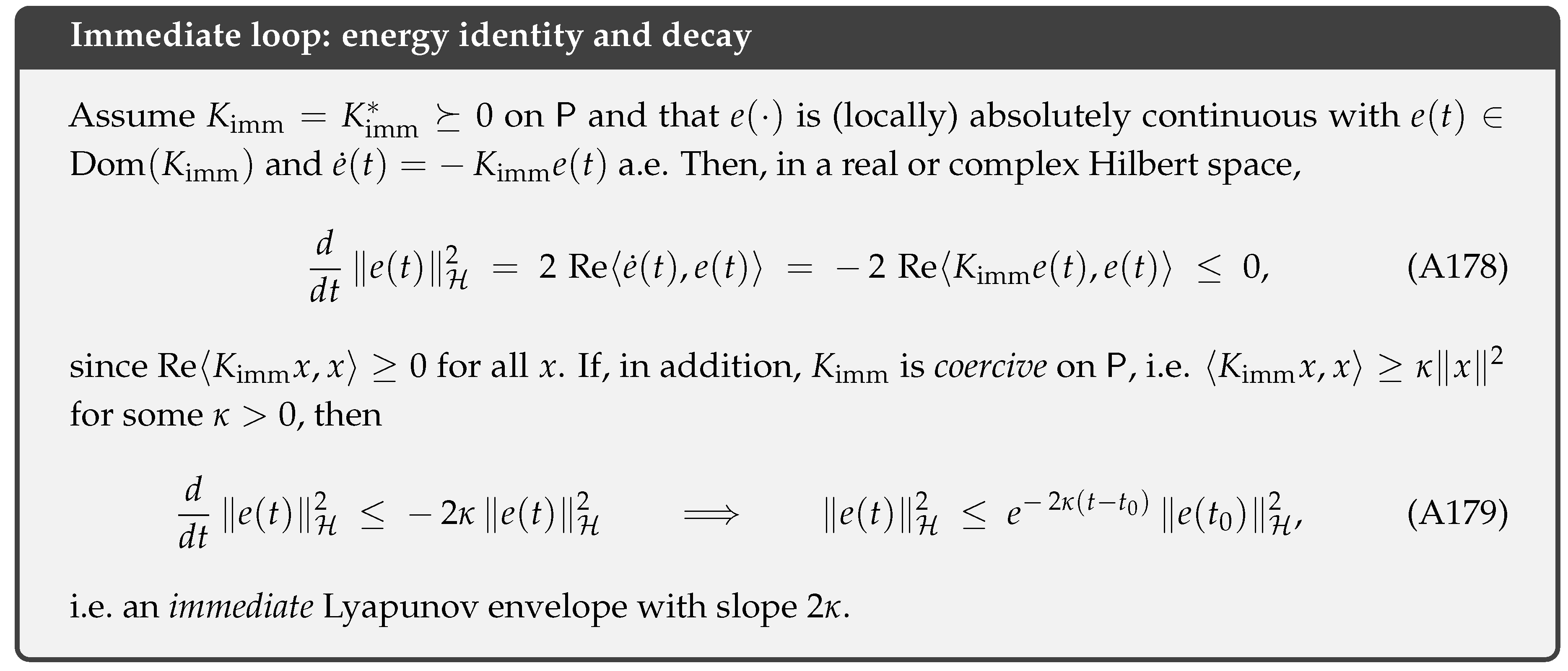
Appendix N.5. Why interchangeability matters

Interchangeability (A173) ensures that the target $\mathcal{I}s$ and the response p are two representations of the same calibrated object in the same geometry. Consequently:

• The residual $R={\parallel p-\mathcal{I}s\parallel }^2$ is exactly the squared energy of e (A175); there is no hidden coupling to other “gauges’’ or spaces.
• A local (or diagonal) $K_{\mathrm{imm}}$ reduces epointwise/modewise, because p and $\mathcal{I}s$ are co-located in $\mathcal{H}$; the loop never needs to “translate’’ between spaces to know which way to push.
• Orthogonal projection identities in $\mathcal{H}$ give the one-line DPI for any admissible processing between steps, complementing the continuous-time decay (A179) [4].

Appendix N.6. Two canonical realizations (educative sketches)

Operator–algebraic (GNS) setting. 

Work in $\mathcal{H}=L^2(\mathcal{M},\omega )$ for a faithful state $\omega$. Take $J^{(+)}$ as the $\omega$-preserving conditional expectation and $\mathcal{I}$ the inclusion; then $\mathcal{I}{J}^{(+)}={\mathrm{id}}_{\mathsf{P}}$, $J^{(+)}\mathcal{I}=P_{\mathsf{S}}$ [3,34,35,36]. Choose $K_{\mathrm{imm}}$ as the positive part of a symmetric Dirichlet form (e.g. the modular/carré-du-champ generator). The energy identity A178) is the standard Dirichlet dissipation; coercivity gives (A179).

PDE (gradient–channel) setting. 

Let $\mathcal{H}=L^2(\Omega ;{\mathbb{R}}^m)$, $e:=p-\mathcal{I}s$, and $\langle K_{\mathrm{imm}}e,e\rangle ={\int }_{\Omega }\langle B\left(x\right)\mathcal{L}e,\mathcal{L}e\rangle dx$, with $B\left(x\right)⪰\beta I$ and $\mathcal{L}$ local (e.g. ∇). Then $\dot{e}=-K_{\mathrm{imm}}e\Rightarrow {\displaystyle \frac{d}{dt}}{\parallel e\parallel }^2=-2\int \langle B\mathcal{L}e,\mathcal{L}e\rangle \le -2\beta {\parallel \mathcal{L}e\parallel }^2$, and a Poincaré/Helmholtz inequality yields (A179) with $\kappa =\beta {\lambda }_1$.

Appendix N.7. Summary

Interchangeability places blueprint and response in the same Hilbert geometry, so the residual is a plain squared norm. If, in that geometry, the generator $K_{\mathrm{imm}}$ is local (or diagonal) and positive (coercive), then each coordinate/mode of e obeys an immediate one–dimensional decay, and the total energy follows by Pythagoras/Parseval. The slow loop ${\int }_0^{t}M(·)e$ encodes delayed, nonlocal corrections; causality throttles that relay across horizons, leaving the immediate loop to enforce the exterior Lyapunov envelope.

Appendix N.8. Propagation identities and Lyapunov envelopes

In the DSFL picture, once statistics and physics are co-located in the same Hilbert geometry, the propagation of the calibrated mismatch $e:=p-\mathcal{I}s$ is most naturally controlled by energy identities and comparison estimates. At this level of generality we do not assume a specific micromodel; we only require a sector–provided evolution law whose instantaneous (local) part is accretive and whose retarded (nonlocal) part is causal and positive. The key outcome is a Lyapunov envelope for the single observable $\mathcal{R}\left(t\right)={\parallel e\left(t\right)\parallel }_{\mathcal{H}}^2$: a differential inequality of the form $\dot{\mathcal{R}}\le -2(\kappa -\epsilon )\mathcal{R}$ implies exponential decay with a rate set by a coercivity margin $\kappa$ (the immediate loop’s gap) up to lower–order leakage $\epsilon$. The next paragraphs record the sector–specific residual identity that yields this envelope and the resulting semilog “straight–line’’ decay for $\mathcal{R}$.

Appendix N.8.1. Residual identity & DSFL–time (sector–specific and time–focused)

Many sectors furnish a differential energy identity for the calibrated mismatch $e:=p-\mathcal{I}s$:

$${\displaystyle \frac{d}{dt}}{\parallel e\left(t\right)\parallel }_{\mathcal{H}}^2=-2{\langle K\left(t\right)e\left(t\right),e\left(t\right)\rangle }_{\mathcal{H}}+2{\langle e\left(t\right),g\left(t\right)\rangle }_{\mathcal{H}},$$

(A180)

with $K\left(t\right)=K{\left(t\right)}^{*}⪰0$ and a lower–order “leakage’’ term bounded by ${|\langle e,g\rangle }_{\mathcal{H}}{|\le \epsilon \left(t\right)\parallel e\parallel }_{\mathcal{H}}^2$. If the sector provides a coercivity/gap margin

$${\langle K\left(t\right)e,e\rangle }_{\mathcal{H}}\ge \kappa \left(t\right){\parallel e\parallel }_{\mathcal{H}}^2(\kappa \left(t\right)\ge 0),$$

(A181)

then the calibrated residual $R\left(t\right):={\parallel e\left(t\right)\parallel }_{\mathcal{H}}^2$ obeys the Lyapunov envelope

$$\dot{R}\left(t\right)\le -2\lambda \left(t\right)R\left(t\right),\lambda \left(t\right):=\kappa \left(t\right)-\epsilon \left(t\right)\ge 0,$$

(A182)

and hence, for all $t\ge t_0$,

$$R\left(t\right)\le exp\left(-2{\int }_{t_0}^t\lambda \left(\tau \right)d\tau \right)R\left(t_0\right).$$

(A183)

Time meaning:$\lambda \left(t\right)$ is the instantaneous rate of the DSFL arrow; the semi–log slope of R is $-2\lambda$.

Appendix N.8.2. Intrinsic DSFL time and unit–slope form

Define the clock–neutral time

$$d\widehat{\tau }:=2\lambda \left(t\right)dt⟹{\displaystyle \frac{dR}{d\widehat{\tau }}}\le -R\Rightarrow R\left(\widehat{\tau }\right)\le e^{-(\widehat{\tau }-{\widehat{\tau }}_0)}R\left({\widehat{\tau }}_0\right).$$

(A184)

Thus every lawful evolution is a unit–slope straight line on semi–log axes in $\widehat{\tau }$, independent of the physical clock.

Appendix N.8.3. Operational arrow (how much time has elapsed)

The accumulated, clock–neutral reduction

$$S_R\left(t\right):=-log{\displaystyle \frac{R\left(t\right)}{R\left(t_0\right)}}={\int }_{t_0}^{t}2\lambda \left(\tau \right)d\tau =\widehat{\tau }\left(t\right)-\widehat{\tau }\left(t_0\right)$$

(A185

quantifies “how much calibrated mismatch was removed’’ and serves as an intrinsic elapsed time in DSFL units.

Appendix N.8.4. Minimal usage (time–centric practitioner checklist)

• Pick the geometry: choose $\mathcal{H}$ that embeds both channels; define $R={\parallel p-\mathcal{I}s\parallel }_{\mathcal{H}}^2$.
• Calibrate: construct $(\mathcal{I},J^{(+)})$ with $\mathcal{I}{J}^{(+)}={\mathrm{id}}_{\mathsf{P}}$, $J^{(+)}\mathcal{I}=P_{\mathsf{S}}$.
• Gate admissibility: verify $\Phi \mathcal{I}=\mathcal{I}\tilde{\Phi }$ and ${\parallel \Phi \parallel }_{\mathcal{H}\to \mathcal{H}}\le 1$ for every update (and mass preservation if using one–budget).
• Read off a rate: identify $\left(\kappa \right(t),\epsilon (t\left)\right)$ in (A180)–(A181); set $\lambda =\kappa -\epsilon$.
• Report time: plot $logR$ vs. physical time t (slope $-2\lambda$) and report $S_R\left(t\right)=-log(R/R_0)$ (elapsed DSFL time).

Appendix N.8.5. Remarks (existence, uniqueness, robustness for time)

• Clock–neutrality: for any strictly increasing $\theta \left(t\right)$, ${\displaystyle \frac{dR}{d\theta }}=(dR/dt)(dt/d\theta )\le 0$; $\widehat{\tau }$ is unique up to affine change.
• Calibration nonuniqueness: results that use only DPI are invariant under any isometry U with $U\left(\mathrm{Im}\mathcal{I}\right)=\mathrm{Im}\mathcal{I}$.
• Local vs nonlocal dynamics: the envelope needs only the gap in (A181); causal/positive memory M is dissipative and cannot worsen decay.
• Discrete consistency: for admissible ticks, $\Delta {\widehat{\tau }}_k=-log(R_{k+1}/R_k)\ge 0$ and $R_n=e^{-({\widehat{\tau }}_n-{\widehat{\tau }}_0)}{R}_0$.

Appendix N.9. Generic two–channel template (plug–and–play for time)

Let $e\left(t\right)=p\left(t\right)-\mathcal{I}s\left(t\right)$, $R\left(t\right)={\parallel e\left(t\right)\parallel }_{\mathcal{H}}^2$. Suppose the sector provides

$$\dot{R}\left(t\right)=-2{\langle Ke,e\rangle }_{\mathcal{H}}+2{\langle e,g\rangle }_{\mathcal{H}},K=K^{*}{⪰0,|\langle e,g\rangle }_{\mathcal{H}}{|\le \epsilon \parallel e\parallel }_{\mathcal{H}}^2,$$

(A186)

and a gap ${\langle Ke,e\rangle }_{\mathcal{H}}\ge \kappa {\parallel e\parallel }_{\mathcal{H}}^2$. Then

$$\dot{R}\left(t\right)\le -2(\kappa -\epsilon )R\left(t\right)⟹R\left(t\right)\le e^{-2(\kappa -\epsilon )(t-t_0)}R\left(t_0\right),$$

(A187)

and in DSFL time $d\widehat{\tau }=2(\kappa -\epsilon )dt$ one has $R\left(\widehat{\tau }\right)\le e^{-(\widehat{\tau }-{\widehat{\tau }}_0)}R\left({\widehat{\tau }}_0\right)$. In parallel, for any admissible $(\tilde{\Phi },\Phi )$,

$$R(\tilde{\Phi }s,\Phi p)\le R(s,p),$$

(A188)

which certifies the direction per step and composes to the continuum envelope.

References

- Wald, R.M. General Relativity; University of Chicago Press: Chicago, 1984. [Google Scholar]
- Hawking, S.W.; Ellis, G.F.R. The Large Scale Structure of Space–Time; Cambridge University Press: Cambridge, 1973. [Google Scholar]
- Ohya, M.; Petz, D. Quantum Entropy and Its Use; Texts and Monographs in Physics, Springer: Berlin, 1993. [Google Scholar] [CrossRef]
- Bauschke, H.H.; Combettes, P.L. Convex Analysis and Monotone Operator Theory in Hilbert Spaces, 2 ed.; CMS Books in Mathematics, Springer: Cham, 2017. [Google Scholar] [CrossRef]
- Gripenberg, G.; Londen, S.O.; Staffans, O. Volterra Integral and Functional Equations; Cambridge University Press: Cambridge, 1990. [Google Scholar]
- Dafermos, M.; Rodnianski, I. The red-shift effect and radiation decay on black hole spacetimes. Communications on Pure and Applied Mathematics 2009, 62, 859–919. [Google Scholar] [CrossRef]
- Berti, E.; Cardoso, V.; Starinets, A.O. Quasinormal modes of black holes and black branes. Classical and Quantum Gravity 2009, 26, 163001. [Google Scholar] [CrossRef]
- Einstein, A. Die Grundlage der allgemeinen Relativitätstheorie. Annalen der Physik 1916, 354, 769–822. [Google Scholar] [CrossRef]
- Breuer, H.P.; Petruccione, F. The Theory of Open Quantum Systems; Oxford University Press, 2002.
- Giddings, S.B. Nonviolent information transfer from black holes: a field theory parametrization. Physical Review D 2013, 88, 064023–1302.2613. [Google Scholar] [CrossRef]
- Harlow, D. Jerusalem Lectures on Black Holes and Quantum Information. Reviews of Modern Physics 2016, 88, 015002–1409.1231. [Google Scholar] [CrossRef]
- Penington, G. Entanglement Wedge Reconstruction and the Information Paradox. Journal of High Energy Physics 2020, 2020, 002–1905.08255. [Google Scholar] [CrossRef]
- Almheiri, A.; Hartman, T.; Maldacena, J.; Shaghoulian, E.; Tajdini, A. The Island Formula for the Entanglement Entropy. Journal of High Energy Physics 2020, 2020, 013–1911.12333. [Google Scholar] [CrossRef]
- Boltzmann, L. Further Studies on the Thermal Equilibrium of Gas Molecules. Sitzungsberichte der Kaiserlichen Akademie der Wissenschaften, Mathematisch-Naturwissenschaftliche Classe 1872, 66, 275–370. [Google Scholar]
- Boltzmann, L. On the Mechanical Theorem of Heat. Annalen der Physik 1896, 60, 392–398. [Google Scholar]
- Loschmidt, J. Über den Zustand des Wärmegleichgewichtes eines Systems von Körpern mit Rücksicht auf die Schwerkraft. Sitzungsberichte der Kaiserlichen Akademie der Wissenschaften 1876, 73, 128–142. [Google Scholar]
- Zermelo, E. Ueber die mechanische Erklärung irreversibler Vorgänge. Annalen der Physik 1896, 293, 485–494. [Google Scholar] [CrossRef]
- Gibbs, J.W. Elementary Principles in Statistical Mechanics; Yale University Press, 1902.
- Lanford, O.E. Time evolution of large classical systems. In Proceedings of the Dynamical Systems, Theory and Applications; Moser, J., Ed., Berlin; 1975; pp. 1–111. [Google Scholar]
- Eddington, A.S. The Nature of the Physical World; Cambridge University Press, 1928.
- Eddington, A.S. The End of the World: From the Standpoint of Mathematical Physics. Nature 1931, 127, 447–453. [Google Scholar] [CrossRef]
- Ehrenfest, P.; Ehrenfest, T. Über zwei bekannte Einwände gegen das Boltzmannsche H–Theorem. Physikalische Zeitschrift 1907, 8, 311–314. [Google Scholar]
- Onsager, L. Reciprocal Relations in Irreversible Processes. I. Physical Review 1931, 37, 405–426. [Google Scholar] [CrossRef]
- Onsager, L. Reciprocal Relations in Irreversible Processes. II. Physical Review 1931, 38, 2265–2279. [Google Scholar] [CrossRef]
- Kubo, R. Statistical-Mechanical Theory of Irreversible Processes. I. Journal of the Physical Society of Japan 1957, 12, 570–586. [Google Scholar] [CrossRef]
- Lindblad, G. On the generators of quantum dynamical semigroups. Communications in Mathematical Physics 1976, 48, 119–130. [Google Scholar] [CrossRef]
- Gorini, V.; Kossakowski, A.; Sudarshan, E.C.G. Completely positive dynamical semigroups of N-level systems. Journal of Mathematical Physics 1976, 17, 821–825. [Google Scholar] [CrossRef]
- Spohn, H. Entropy production for quantum dynamical semigroups. Journal of Mathematical Physics 1978, 19, 1227–1230. [Google Scholar] [CrossRef]
- Davies, E.B. Quantum Theory of Open Systems; Academic Press: London; New York, 1976. First edition.
- Lindblad, G. Completely Positive Maps and Entropy Inequalities. Communications in Mathematical Physics 1975, 40, 147–151. [Google Scholar] [CrossRef]
- Uhlmann, A. Relative entropy and the Wigner–Yanase–Dyson–Lieb concavity in an interpolation theory. Communications in Mathematical Physics 1977, 54, 21–32. [Google Scholar] [CrossRef]
- Lieb, E.H.; Ruskai, M.B. Proof of the strong subadditivity of quantum-mechanical entropy. Journal of Mathematical Physics 1973, 14, 1938–1941. [Google Scholar] [CrossRef]
- Petz, D. Monotonicity of Quantum Relative Entropy. Reviews in Mathematical Physics 2003, 15, 79–91. [Google Scholar] [CrossRef]
- Takesaki, M. Conditional Expectations in von Neumann Algebras. Journal of Functional Analysis 1972, 9, 306–321. [Google Scholar] [CrossRef]
- Takesaki, M. Theory of Operator Algebras II; Vol. 125, Encyclopaedia of Mathematical Sciences, Springer: Berlin, 2003. [Google Scholar] [CrossRef]
- Tomiyama, J. On the Projection of Norm One in W*-Algebras. Proceedings of the Japan Academy 1957, 33, 608–612. [Google Scholar] [CrossRef]
- Stinespring, W.F. Positive Functions on C*-Algebras. Proceedings of the American Mathematical Society 1955, 6, 211–216. [Google Scholar]
- Kraus, K. General state changes in quantum theory. Annals of Physics 1971, 64, 311–335. [Google Scholar] [CrossRef]
- Bhatia, R. Matrix Analysis; Vol. 169, Graduate Texts in Mathematics, Springer: New York, 1997. [Google Scholar] [CrossRef]
- Cover, T.M.; Thomas, J.A. Elements of Information Theory, 2 ed.; Wiley Series in Telecommunications and Signal Processing; Wiley: Hoboken, NJ, 2006. [Google Scholar] [CrossRef]
- Jarzynski, C. Nonequilibrium Equality for Free Energy Differences. Physical Review Letters 1997, 78, 2690–2693. [Google Scholar] [CrossRef]
- Crooks, G.E. Entropy production fluctuation theorem and the nonequilibrium work relation for free energy differences. Physical Review E 1999, 60, 2721–2726. [Google Scholar] [CrossRef]
- Evans, D.J.; Searles, D.J. The Fluctuation Theorem. Advances in Physics 2002, 51, 1529–1585. [Google Scholar] [CrossRef]
- Gallavotti, G.; Cohen, E.G.D. Dynamical Ensembles in Nonequilibrium Statistical Mechanics. Physical Review Letters 1995, 74, 2694–2697. [Google Scholar] [CrossRef]
- Seifert, U. Stochastic thermodynamics, fluctuation theorems and molecular machines. Reports on Progress in Physics 2012, 75, 126001. [Google Scholar] [CrossRef]
- Esposito, M.; Harbola, U.; Mukamel, S. Nonequilibrium fluctuations, fluctuation theorems, and counting statistics in quantum systems. Reviews of Modern Physics 2009, 81, 1665–1702. [Google Scholar] [CrossRef]
- Lieb, E.H.; Robinson, D.W. The finite group velocity of quantum spin systems. Communications in Mathematical Physics 1972, 28, 251–257. [Google Scholar] [CrossRef]
- Nachtergaele, B.; Sims, R. Lieb–Robinson bounds and the exponential clustering theorem. Communications in Mathematical Physics 2006, 265, 119–130. [Google Scholar] [CrossRef]
- Hastings, M.B. Locality in quantum and Markov dynamics on lattices and networks. Physical Review Letters 2004, 93, 140402. [Google Scholar] [CrossRef]
- Bauerschmidt, R.; Brydges, D.C.; Slade, G. Introduction to a Renormalisation Group Method; Vol. 2242, Lecture Notes in Mathematics, Springer, 2021. [CrossRef]
- Einstein, A. Die Feldgleichungen der Gravitation. Sitzungsberichte der Preussischen Akademie der Wissenschaften, 1915; 844–847. [Google Scholar]
- Hawking, S.W. Gravitational radiation from colliding black holes. Physical Review Letters 1971, 26, 1344–1346. [Google Scholar] [CrossRef]
- Bekenstein, J.D. Black holes and entropy. Physical Review D 1973, 7, 2333–2346. [Google Scholar] [CrossRef]
- Hawking, S.W.; King, A.R.; McCarthy, P.J. A New Topology for Curved Space-time which Incorporates the Causal, Differential, and Conformal Structures. Journal of Mathematical Physics 1976, 17, 174–181. [Google Scholar] [CrossRef]
- Unruh, W.G. Notes on black-hole evaporation. Physical Review D 1976, 14, 870–892. [Google Scholar] [CrossRef]
- Dafermos, M.; Rodnianski, I. A new physical-space approach to decay for the wave equation, 2010. arXiv:0910.4957.
- Dafermos, M.; Rodnianski, I. The red-shift effect and radiation decay on black hole spacetimes. Communications on Pure and Applied Mathematics 2010, 62, 859–919. [Google Scholar] [CrossRef]
- Penrose, R. Singularities and time-asymmetry. In General Relativity: An Einstein Centenary Survey; Hawking, S.W.; Israel, W., Eds.; Cambridge University Press, 1979; pp. 581–638.
- Carroll, S. From Eternity to Here The Quest for the Ultimate Theory of Time; Dutton, 2010.
- Page, D.N. Average Entropy of a Subsystem. Physical Review Letters 1993, 71, 1291–1294. [Google Scholar] [CrossRef] [PubMed]
- Mathur, S.D. The Information Paradox: A Pedagogical Introduction. Classical and Quantum Gravity 2009, arXiv:hep-th/0909.1038]26, 224001. [Google Scholar] [CrossRef]
- Almheiri, A.; Marolf, D.; Polchinski, J.; Sully, J. Black Holes: Complementarity or Firewalls? Journal of High Energy Physics 2013, arXiv:hep-th/1207.3123]2013, 062. [Google Scholar] [CrossRef]
- Susskind, L.; Thorlacius, L.; Uglum, J. The Stretched Horizon and Black Hole Complementarity. Physical Review D 1993, 48, 3743–3761. [Google Scholar] [CrossRef] [PubMed]
- ’t Hooft, G. Dimensional reduction in quantum gravity. arXiv preprint, 1993. [Google Scholar]
- Wald, R.M. Quantum Field Theory in Curved Spacetime and Black Hole Thermodynamics; University of Chicago Press, 1994.
- Kadison, R.V. A generalized Schwarz inequality and algebraic invariants for operator algebras. Annals of Mathematics 1952, 56, 494–503. [Google Scholar] [CrossRef]