Modeling the Non Markovian Dynamics of Open Quantum System Strongly Coupled to Reservoirs Through Quantum Master Equation by Method of Reaction Coordinate Mapping and the Mesoscopic Lead Construction

1. Introduction

The standard formulation of thermodynamics is based around the assumption of vanishingly weak interactions between the system of interest and any thermal reservoirs to which it is attached. Under these conditions, a system that is put into contact with a single heat reservoir will customarily thermalise to a canonical Gibbs state, with the reservoir itself assumed to remain in thermal equilibrium at a given temperature. A weak coupling approximation is generally very well justified on macroscopic scales, whereby only a small fraction of the system and reservoir constituent degrees of freedom are usually in contact. On nanoscale, however, such a simplification becomes much more questionable, perhaps particularly so when the system and reservoir are quantum mechanical in nature and the generation of non-classical correlations between the two may then play a prominent role. Several attempts have therefore been made to move beyond weak coupling in this context. The idea of the reaction coordinate mapping is extremely useful when someone is interested to study the dynamics of the system which is strongly coupled to the bath or, surroundings. This introduces memory effect and non markovian evolution of the system though the dynamics of the extended system obtained after the markovian embedding is markovian in nature. The quantum master equation after the reaction coordinate mapping has also been derived for both the case of weak and strong coupling case between the system and the reaction coordinates. In this article the sections deals with the mathematical derivations of the results related to the Reaction coordinate mapping for different situations. The aspects of the mesoscopic lead construction has also been discussed in the later section.

2. Reaction Coordinate Mapping

Let us consider the hamiltonian of the supersystem describing the interaction of a quantum system coupled with a single bath described by,

$$\begin{array}{c}\widehat{H}={\widehat{H}}_S+{\widehat{H}}_B+{\widehat{H}}_{SB}\end{array}$$

(1)

$$\begin{array}{c}{\widehat{H}}_B=\sum _m{\nu }_m{\widehat{c}}_m^{†}{\widehat{c}}_m\end{array}$$

(2)

$$\begin{array}{c}{\widehat{H}}_{SB}=\widehat{S}\sum _m{g}_m({\widehat{c}}_m+{\widehat{c}}_m^{†})\end{array}$$

(3)

The bath spectral function can be defined as,

$$J_0\left(\omega \right)=2\pi \sum _m{\left|g_m\right|}^2\delta (\omega -{\nu }_m)$$

(4)

Let us consider an example of Reaction coordinate mapping before returning to the present context. Let us consider a quantum system coupled to a bath which itself has infinite number of degrees of freedom described by infinite number of bath modes (energy levels) with each of them is represented by a harmonic oscillator. With $\widehat{s}$ being any arbitrary system operator the Hamiltonian of the entire supersystem i.e. system coupled to the bath can be written as,

$$\widehat{H}={\widehat{H}}_S\left(t\right)+{\displaystyle \frac{1}{2}}\sum _m\left[{\widehat{p}}_m^2+{\nu }_m^2{\left({\widehat{x}}_m-{\displaystyle \frac{c_m}{{\nu }_m^2}}\widehat{S}\right)}^2\right]$$

(5)

In general the system Hamiltonian can be time independent. After decomposing the above Hamiltonian we get,

$$\begin{array}{c}\widehat{H}={\widehat{H}}_S\left(t\right)+{\widehat{S}}^2\sum _m{\displaystyle \frac{c_m^2}{{\omega }_m^2}}+{\widehat{H}}_B+{\widehat{H}}_{SB}\end{array}$$

(6)

$$\begin{array}{c}{\widehat{H}}_B={\displaystyle \frac{1}{2}}\sum _m\left[{\widehat{p}}_m^2+{\nu }_m^2{\widehat{x}}_m^2\right]\end{array}$$

(7)

$$\begin{array}{c}{\widehat{H}}_{SB}=-\widehat{S}\sum _m{c}_m{\widehat{x}}_m\end{array}$$

(8)

The usual commutation relations are,

$$\left[{\widehat{x}}_m,{\widehat{x}}_n\right]=0=\left[{\widehat{p}}_m,{\widehat{p}}_n\right]\mathrm{and}\left[{\widehat{x}}_m,{\widehat{p}}_n\right]=i\widehat{\hslash }{\delta }_{mn}\widehat{I}$$

(9)

Let us define the spectral function of the bath as,

$$J_0\left(\omega \right)={\displaystyle \frac{\pi }{2}}\sum _m{\displaystyle \frac{c_m^2}{{\nu }_m}}\delta (\omega -{\nu }_m)$$

(10)

Figure 1. Reaction Coordinate mapping

Figure 1. Reaction Coordinate mapping

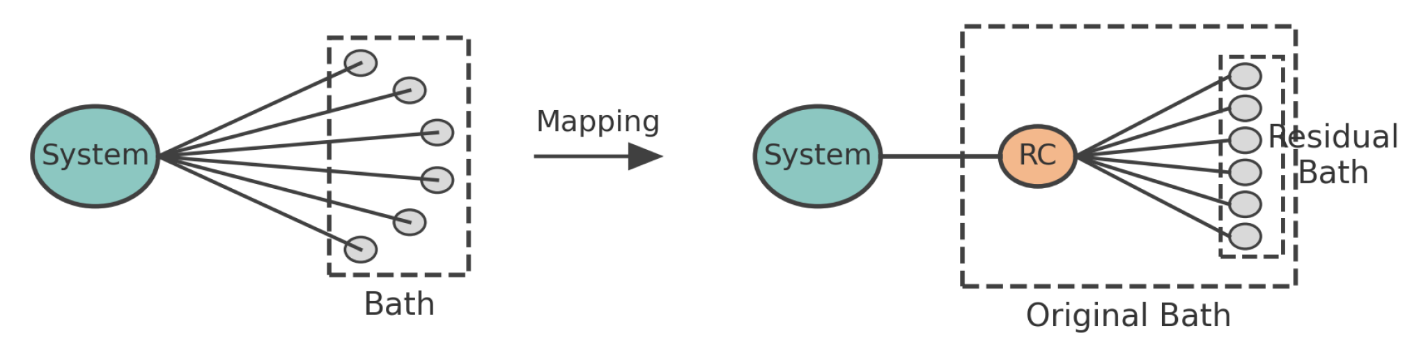
Now let us consider the Reaction Coordinate mapping as shown in the figure which enables us to separate one of the modes called the reaction mode or reaction coordinate from the infinite number of bath modes such that the system is now interacting with that particular segregated reaction coordinate which in turn coupled to the rest of the modes of the bath which we call residual bath modes. In this way we can visualise the system is interacting with one reaction coordinate which is connected or coupled to the residual bath. The situation after one such steps of Reaction coordinate mapping the hamiltonian will be as follows,

$$\begin{array}{c}{\widehat{H}}_{\mathcal{R}}={\widehat{U}}_{\mathcal{R}}\widehat{H}{\widehat{U}}_{\mathcal{R}}^{†}\end{array}$$

(11)

$$\begin{array}{c}{\widehat{H}}_{\mathcal{R}}={\widehat{H}}_S\left(t\right)+{\displaystyle \frac{\delta {\mathrm{\Omega }}_0^2}{2}}{\widehat{S}}^2+{\widehat{H}}_{RC}+{\widehat{H}}_{S-RC}+{\widehat{H}}_{RE}+{\widehat{H}}_{RC-RE}\end{array}$$

(12)

$$\begin{array}{c}{\widehat{H}}_{RC}={\displaystyle \frac{1}{2}}\left[{\widehat{P}}_1^2+{\omega }_1^2{\widehat{X}}_1^2\right]\end{array}$$

(13)

$$\begin{array}{c}{\widehat{H}}_{S-RC}=-{\lambda }_0\widehat{S}{\widehat{X}}_1\end{array}$$

(14)

$$\begin{array}{c}{\widehat{H}}_{RE}={\displaystyle \frac{1}{2}}\sum _{m\ne 1}\left[{\widehat{P}}_m^2+{\omega }_m^2{\widehat{X}}_m^2\right]\end{array}$$

(15)

$$\begin{array}{c}{\widehat{H}}_{RC-RE}=-{\widehat{X}}_1\sum _{m\ne 1}{C}_m{\widehat{X}}_m\end{array}$$

(16)

${\widehat{H}}_{\mathcal{R}}$ describes the Hamiltonian of the system after one step of reaction coordinate mapping which can be treated as an unitary transformation of the Hamiltonian before the RC mapping i.e. $\widehat{H}$. Now, the exactness of the mapping which depicts the equivalence between the situation before and after the reaction coordinate mapping is given by,

$${\lambda }_0\widehat{S}{\widehat{X}}_1=\widehat{S}\sum _m{c}_m{\widehat{x}}_m\Rightarrow {\lambda }_0{\widehat{X}}_1=\sum _m{c}_m{x}_m$$

(17)

The above reaction coordinate mapping can be visualized as a transformation from one set of normal modes (coordinates) say $({\widehat{x}}_1,{\widehat{x}}_2,...,{\widehat{x}}_n;{\widehat{p}}_1,{\widehat{p}}_2,...,{\widehat{p}}_n)$ to $({\widehat{X}}_1,{\widehat{X}}_2,...,{\widehat{X}}_n;{\widehat{P}}_1,{\widehat{P}}_2,...,{\widehat{P}}_n)$ defined by an orthogonal transformation the later being required to preserve the usual commutation relations of the newly defined normal mode coordinates. And as the bath has been represented by infinite number of modes in a discreet sense then later we will take the thermodynamic limit i.e. $n\to \infty$. Let us define the following transformation $\widehat{\mathbf{X}}=\mathrm{\Lambda }\widehat{\mathbf{x}}$ and $\widehat{\mathbf{P}}=\mathrm{\Lambda }\widehat{\mathbf{p}}$ with a claim that $\mathrm{\Lambda }$ has to be an orthogonal matrix which we are going to derive. From now on-wards we will use the natural unit system with $\hslash =k_B=c=1$.

$$\begin{array}{c}\mathrm{We}\mathrm{need}\left[{\widehat{X}}_m,{\widehat{X}}_n\right]=0=\left[{\widehat{P}}_m,{\widehat{P}}_n\right]\mathrm{with}\left[{\widehat{X}}_m,{\widehat{P}}_n\right]=i{\delta }_{mn}\widehat{I}\end{array}$$

(18)

$$\begin{array}{c}\left[{\widehat{X}}_m,{\widehat{X}}_n\right]=\sum _{\alpha }\sum _{\beta }{\mathrm{\Lambda }}_{m\alpha }{\mathrm{\Lambda }}_{n\beta }\left[{\widehat{x}}_{\alpha },{\widehat{x}}_{\beta }\right]=0\end{array}$$

(19)

$$\begin{array}{c}\mathrm{similarly}\left[{\widehat{P}}_m,{\widehat{P}}_n\right]=\sum _{\alpha }\sum _{\beta }{\mathrm{\Lambda }}_{m\alpha }{\mathrm{\Lambda }}_{n\beta }\left[{\widehat{p}}_{\alpha },{\widehat{p}}_{\beta }\right]=0\end{array}$$

(20)

$$\begin{array}{c}\left[{\widehat{X}}_m,{\widehat{P}}_n\right]=\sum _{\alpha }\sum _{\beta }{\mathrm{\Lambda }}_{m\alpha }{\mathrm{\Lambda }}_{n\beta }\left[{\widehat{x}}_{\alpha },{\widehat{p}}_{\beta }\right]=i\sum _{\alpha }\sum _{\beta }{\mathrm{\Lambda }}_{m\alpha }{\mathrm{\Lambda }}_{n\beta }{\delta }_{\alpha \beta }\end{array}$$

(21)

$$\begin{array}{c}\left[{\widehat{X}}_m,{\widehat{P}}_n\right]=i{\delta }_{mn}\Rightarrow \sum _{\alpha }{\mathrm{\Lambda }}_{m\alpha }{\mathrm{\Lambda }}_{n\alpha }={\delta }_{mn}\Rightarrow \sum _{\alpha }{\left(\mathrm{\Lambda }\right)}_{m\alpha }{\left({\mathrm{\Lambda }}^T\right)}_{\alpha n}={\mathbf{I}}_{mn}\end{array}$$

(22)

Hence we can see that to preserve the commutation relations of the newly defined set of normal mode coordinates i.e. $({\widehat{X}}_{\alpha },{\widehat{P}}_{\beta })$ the transformation has to be orthogonal with $\mathrm{\Lambda }{\mathrm{\Lambda }}^T={\mathrm{\Lambda }}^T\mathrm{\Lambda }=\mathbf{I}$. The condition of orthogonality along with ${\lambda }_0{\widehat{X}}_1={\sum }_m{c}_m{\widehat{x}}_m$ leads to,

$$\begin{array}{c}\mathrm{with}{\widehat{X}}_1=\sum _{\alpha }{\mathrm{\Lambda }}_{1\alpha }{\widehat{x}}_{\alpha }\end{array}$$

(23)

$$\begin{array}{c}{\lambda }_0\sum _{\alpha }{\mathrm{\Lambda }}_{1\alpha }{\widehat{x}}_{\alpha }=\sum _{\alpha }{c}_{\alpha }{\widehat{x}}_{\alpha }\Rightarrow {\lambda }_0{\mathrm{\Lambda }}_{1\alpha }=c_{\alpha }\end{array}$$

(24)

$$\begin{array}{c}{\lambda }_0^2\sum _{\alpha }{\mathrm{\Lambda }}_{1\alpha }^2=\sum _{\alpha }{c}_{\alpha }^2\mathrm{with}\sum _{\alpha }{\mathrm{\Lambda }}_{1\alpha }^2=1.\Rightarrow \begin{array}{|c|}\hline {\lambda }_0^2={\displaystyle \sum _{\alpha }}{c}_{\alpha }^2\\ \hline\end{array}\end{array}$$

(25)

Now applying the inverse orthogonal transformation by writing ${\widehat{x}}_m={\sum }_{\alpha }{\mathrm{\Lambda }}_{\alpha m}{\widehat{X}}_{\alpha }$ and ${\widehat{p}}_m={\sum }_{\alpha }{\mathrm{\Lambda }}_{\alpha m}{\widehat{P}}_{\alpha }$ the hamiltonian becomes,

$$\begin{array}{c}\widehat{H}={\widehat{H}}_S\left(t\right)+{\displaystyle \frac{\delta {\mathrm{\Omega }}_0^2}{2}}{\widehat{S}}^2-{\lambda }_0\widehat{S}{\widehat{X}}_1+{\displaystyle \frac{1}{2}}\left[{\widehat{P}}_1^2+{\omega }_1^2{\widehat{X}}_1^2\right]+{\displaystyle \frac{1}{2}}\sum _{m\ne 1}\left[{\widehat{P}}_m^2+{\omega }_m^2{\widehat{X}}_m^2\right]-{\widehat{X}}_1\sum _{m\ne 1}{C}_m{\widehat{X}}_m\end{array}$$

(26)

$$\begin{array}{c}\mathrm{where}\delta {\mathrm{\Omega }}_0^2=\sum _m{\displaystyle \frac{c_m^2}{{\nu }_m^2}}=\sum _m{\nu }_m^{-2}{c}_m^2\end{array}$$

(27)

The mathematical deduction of the above is as follows.

$$\begin{array}{c}\sec \mathrm{ond}\mathrm{term}\text{:}{\displaystyle \frac{1}{2}}\sum _m\left[{\widehat{p}}_m^2+{\nu }_m^2{\widehat{x}}_m^2\right]\to {\displaystyle \frac{1}{2}}\sum _m\sum _{\alpha }\sum _{\beta }{\mathrm{\Lambda }}_{\alpha m}{\mathrm{\Lambda }}_{\beta m}{\widehat{P}}_{\alpha }{\widehat{P}}_{\beta }+{\displaystyle \frac{1}{2}}\sum _m\sum _{\alpha }\sum _{\beta }{\nu }_m^2{\mathrm{\Lambda }}_{\alpha m}{\mathrm{\Lambda }}_{\beta m}{\widehat{X}}_{\alpha }{\widehat{X}}_{\beta }\\ ={\displaystyle \frac{1}{2}}\sum _{\alpha }\sum _{\beta }{\widehat{P}}_{\alpha }{\widehat{P}}_{\beta }{\delta }_{\alpha \beta }+{\displaystyle \frac{1}{2}}\sum _m{\nu }_m^2{\mathrm{\Lambda }}_{1m}^2{\widehat{X}}_1^2+{\displaystyle \frac{1}{2}}\sum _m\sum _{\alpha \ne 1}{\nu }_m^2{\mathrm{\Lambda }}_{\alpha m}^2{\widehat{X}}_{\alpha }^2\\ +\sum _m\sum _{\alpha \ne 1}{\nu }_m^2{\mathrm{\Lambda }}_{\alpha m}{\mathrm{\Lambda }}_{1m}{\widehat{X}}_{\alpha }{\widehat{X}}_1+\sum _m\sum _{\begin{array}{c}\alpha ,\beta \\ \alpha \ne \beta \end{array}}{\nu }_m^2{\mathrm{\Lambda }}_{\alpha m}{\mathrm{\Lambda }}_{\beta m}{\widehat{X}}_{\alpha }{\widehat{X}}_{\beta }\\ ={\displaystyle \frac{1}{2}}\left[{\widehat{P}}_1^2+{\omega }_1^2{\widehat{X}}_1^2\right]+{\displaystyle \frac{1}{2}}\sum _{m\ne 1}\left[{\widehat{P}}_m^2+{\omega }_m^2{\widehat{X}}_m^2\right]-{\widehat{X}}_1\sum _m{C}_m{\widehat{X}}_m\\ \mathrm{interaction}\mathrm{term}\text{:}\widehat{S}\sum _m{c}_m{\widehat{x}}_m=\widehat{S}\sum _m\sum _{\alpha }{c}_m{\mathrm{\Lambda }}_{\alpha m}{\widehat{X}}_{\alpha }=\widehat{S}\sum _m{c}_m{\mathrm{\Lambda }}_{1m}{\widehat{X}}_1+\widehat{S}\sum _m\sum _{\alpha \ne 1}{c}_m{\mathrm{\Lambda }}_{\alpha m}{\widehat{X}}_{\alpha }\to {\lambda }_0\widehat{S}{\widehat{X}}_1\\ \mathrm{with}\widehat{H}\to {\widehat{H}}_{\mathcal{R}}={\widehat{H}}_S\left(t\right)+{\displaystyle \frac{\delta {\mathrm{\Omega }}_0^2}{2}}{\widehat{S}}^2+{\displaystyle \frac{1}{2}}\left[{\widehat{P}}_1^2+{\omega }_1^2{\widehat{X}}_1^2\right]+{\displaystyle \frac{1}{2}}\sum _{m\ne 1}\left[{\widehat{P}}_m^2+{\omega }_m^2{\widehat{X}}_m^2\right]-{\lambda }_0\widehat{S}{\widehat{X}}_1-{\widehat{X}}_1\sum _m{C}_m{\widehat{X}}_m\end{array}$$

Using the fact that, ${\lambda }_0{\mathrm{\Lambda }}_{1m}=c_m$ we get,

$${\lambda }_0^2{\omega }_1^2=\sum _m{\nu }_m^2{c}_m^2$$

(28)

where we have identified the following,

$$\begin{array}{c}\delta {\mathrm{\Omega }}_0^2=\sum _m{c}_m^2{\nu }_m^{-2}\\ {\omega }_1^2=\sum _m{\nu }_m^2{\mathrm{\Lambda }}_{1m}^2\\ {\omega }_m^2=\sum _{\alpha }{\nu }_{\alpha }^2{\mathrm{\Lambda }}_{m\alpha }^2\mathrm{for}m\ne 1\\ \mathrm{for}m\ne n\mathrm{we}\mathrm{have}\sum _{\alpha }{\nu }_{\alpha }^2{\mathrm{\Lambda }}_{m\alpha }{\mathrm{\Lambda }}_{n\alpha }=0\\ \mathrm{together}\mathrm{we}\mathrm{get}\sum _{\alpha }{\nu }_{\alpha }^2{\mathrm{\Lambda }}_{m\alpha }{\mathrm{\Lambda }}_{n\alpha }={\omega }_m^2{\delta }_{mn}\end{array}$$

Now, by using the definition of the Bath spectral function i.e. $J_0\left(\omega \right)$ we can express the new parameters mainly, ${\lambda }_0,{\omega }_1,\delta {\mathrm{\Omega }}_0^2$ in terms of the old bath spectral function i.e. the one we have defined before the Reaction Coordinate mapping. Just to note that, ${\lambda }_0$ defines the new system-bath coupling strength alternatively we can call it the coupling strength quantifying the interaction between the system and the reaction coordinate. Similarly, ${\omega }_1$ defines the frequency of the Reaction coordinate. The idea is to express the newly defined quantities in terms of the older (known) quantities. We have defined,

$$J_0\left(\omega \right)={\displaystyle \frac{\pi }{2}}\sum _m{c}_m^2\delta (\omega -{\nu }_m)$$

(29)

We get,

$$\begin{array}{c}\delta {\mathrm{\Omega }}_0^2={\displaystyle \frac{2}{\pi }}{\int }_0^{\infty }{\displaystyle \frac{J_0\left(\omega \right)}{\omega }}d\omega \end{array}$$

(30)

$$\begin{array}{c}{\lambda }_0^2=\sum _m{c}_m^2={\displaystyle \frac{2}{\pi }}{\int }_0^{\infty }\omega J_0\left(\omega \right)d\omega \end{array}$$

(31)

$$\begin{array}{c}{\lambda }_0^2{\omega }_1^2={\displaystyle \frac{2}{\pi }}{\int }_0^{\infty }{\omega }^3{J}_0\left(\omega \right)d\omega \Rightarrow {\omega }_1^2={\displaystyle \frac{2}{\pi {\lambda }_0^2}}{\int }_0^{\infty }{\omega }^3{J}_0\left(\omega \right)d\omega \end{array}$$

(32)

$$\begin{array}{c}{\omega }_1^2={\displaystyle \frac{{\int }_0^{\infty }{\omega }^3{J}_0\left(\omega \right)d\omega }{{\int }_0^{\infty }\omega J_0\left(\omega \right)d\omega }}\end{array}$$

(33)

One important property of this RC mapping is the Scaling transformation property. If the interaction coefficient $c_m$ is transformed to $\alpha c_m,\alpha \in \mathbb{R}$ before the reaction coordinate mapping then only ${\lambda }_0$ and $\delta {\mathrm{\Omega }}_0^2$ will be affected by this scaling transformation. To show it mathematically we can write,

$$\begin{array}{c}{\lambda }_0{\mathrm{\Lambda }}_{1m}=c_m\mapsto {\lambda }_0{\mathrm{\Lambda }}_{1m}=\alpha c_m\mathrm{such}\mathrm{that}{\lambda }_0^2={\alpha }^2\sum _m{c}_m^2\end{array}$$

(34)

$$\begin{array}{c}{\lambda }_0^2={\displaystyle \frac{2{\alpha }^2}{\pi }}{\int }_0^{\infty }\omega J_0\left(\omega \right)d\omega \end{array}$$

(35)

$$\begin{array}{c}\delta {\mathrm{\Omega }}_0^2=\sum _m{\displaystyle \frac{c_m^2}{{\nu }_m^2}}⟼{\alpha }^2\sum _m{\nu }_m^{-2}{c}_m^2={\displaystyle \frac{2{\alpha }^2}{\pi }}{\int }_0^{\infty }{\displaystyle \frac{J_0\left(\omega \right)}{\omega }}d\omega \end{array}$$

(36)

$$\begin{array}{c}{\omega }_1^2=\sum _m{\nu }_m^2{\mathrm{\Lambda }}_{1m}^2\mapsto {\lambda }_0^2{\omega }_1^2={\alpha }^2\sum _m{\nu }_m^2{c}_m^2\Rightarrow {\displaystyle \frac{2{\alpha }^2{\omega }_1^2}{{\pi }^2}}{\int }_0^{\infty }\omega J_0\left(\omega \right)d\omega ={\displaystyle \frac{2{\alpha }^2}{\pi }}{\int }_0^{\infty }{\omega }^3{J}_0\left(\omega \right)d\omega \end{array}$$

(37)

$$\begin{array}{c}{\omega }_1^2={\displaystyle \frac{{\int }_0^{\infty }{\omega }^3{J}_0\left(\omega \right)d\omega }{{\int }_0^{\infty }\omega J_0\left(\omega \right)d\omega }}\end{array}$$

(38)

From the above calculation it is evident that the on site energy of the reaction coordinate i.e. ${\omega }_1$ remains unaffected by the scaling parameter $\alpha$. Similarly we can show that the new coupling coefficient describing the coupling between the reaction coordinate and residual reservoir will be unaffected by the parameter $\alpha$. Now let us define the spectral function of the residual bath or residual reservoir as,

$$J_1\left(\omega \right)={\displaystyle \frac{\pi }{2}}\sum _m{C}_m^2\delta (\omega -{\omega }_m)$$

(39)

Now the job is to express the spectral function of the residual bath i.e. $J_1\left(\omega \right)$ with the older bath spectral function (one before the RC mapping) i.e. $J_0\left(\omega \right)$.

Now we would like to extend the above idea of reaction coordinate mapping in the general situation described by,

$$\begin{array}{c}\widehat{H}={\widehat{H}}_S+{\widehat{H}}_B+{\widehat{H}}_{SB}\\ {\widehat{H}}_B=\sum _m{\nu }_m{\widehat{c}}_m^{†}{\widehat{c}}_m\\ {\widehat{H}}_{SB}=\widehat{S}\sum _m{g}_m({\widehat{c}}_m+{\widehat{c}}_m^{†})\end{array}$$

Where, $\widehat{S}$ being any arbitrary hermitian operator corresponding to the system. An alternative scenario of the system bath coupling can be described by,

$${\widehat{H}}_{SB}=\sum _m(g_m{\widehat{S}}^{†}{\widehat{c}}_m+g_m^{*}\widehat{S}{\widehat{c}}_m^{†})$$

(40)

. In this situation $\widehat{S}$ is non-hermitian. Lets illustrate it by an example with the spin boson model hamiltonian dsescribed by,

$$\begin{array}{c}{\widehat{H}}_1={\displaystyle \frac{{\omega }_0}{2}}{\widehat{\sigma }}_z+\sum _m{\nu }_m{\widehat{c}}_m^{†}{\widehat{c}}_m+{\widehat{\sigma }}_x\sum _m{g}_m({\widehat{c}}_m^{†}+{\widehat{c}}_m)\end{array}$$

(41)

$$\begin{array}{c}{\widehat{H}}_2={\displaystyle \frac{{\omega }_0}{2}}{\widehat{\sigma }}_z+\sum _m{\nu }_m{\widehat{c}}_m^{†}{\widehat{c}}_m+\sum _m(g_m{\widehat{\sigma }}^{+}{\widehat{c}}_m+g_m^{*}{\widehat{\sigma }}^{-}{\widehat{c}}_m^{†})\end{array}$$

(42)

The hamiltonians ${\widehat{H}}_1$ and ${\widehat{H}}_2$ describes the above two situations. The only difference between the two hamiltonians is that for the first case scenario with ${\widehat{H}}_1$ does not commute with the total excitation number operator i.e. ${\widehat{N}}_{exc}={\widehat{\sigma }}^{+}{\widehat{\sigma }}^{-}+{\sum }_m{\widehat{c}}_m^{†}{\widehat{c}}_m$ which means that ${\widehat{N}}_{exc}$ is not a conserved quantity in this case. But in the second case we can write, $\left[{\widehat{H}}_2,{\widehat{N}}_{exc}\right]=0$ which means that ${\widehat{N}}_{exc}$ is a conserved quantity which is the outcome of the Global U(1) symmetry. Now we can define the normal mode coordinate transformation as follows,

$$\begin{array}{c}{\widehat{c}}_m=u_{mq}{\widehat{b}}_q+v_{mq}{\widehat{b}}_q^{†}\end{array}$$

(43)

$$\begin{array}{c}{c}_m^{†}=u_{mq}*{\widehat{b}}_q^{†}+v_{mq}^{*}{\widehat{b}}_q\end{array}$$

(44)

This kind of transformation is called a symplectic transformation. There is another way to define the transformation defined as,

$$\begin{array}{c}{\widehat{c}}_m=u_{mq}{\widehat{b}}_q\mathrm{and}{c}_m^{†}=u_{mq}^{*}{\widehat{b}}_q^{†}\end{array}$$

(45)

The difference between the transformations of two kinds are noteworthy. In the first case the transformation mix up the creation and annihilation operators of the bath modes before and after the reaction coordinate mapping where as in the second case such mixing doesn’t happen. The later case is just an unitary transformation. The condition of unitarity and symplecticity are hereby imposed to preserve the commutation (anti-commutation) relations of the bosonic (fermionic) creation and annihilation operators.

Derivation of Symplecticity and Unitarity: For bosons and fermionic mapping case we must have,

$${\left[{\widehat{c}}_m,{\widehat{c_n}}^{†}\right]}_{\pm }={\delta }_{mn}\mathrm{with}{\left[{\widehat{b}}_{\alpha },{\widehat{b}}_{\beta }^{†}\right]}_{\pm }={\delta }_{\alpha \beta }$$

(46)

The condition essentially preserve the necessary commutation (anti-commutation) relations for the bosonic and fermionic mapping case for the creation and annihilation operators corresponding to the new and older normal modes. We have defined in general for any two operator $\widehat{A}$ and $\widehat{B}$,

$${\left[\widehat{A},\widehat{B}\right]}_{\pm }=\left[\widehat{A}\widehat{B}\pm \widehat{B}\widehat{A}\right]$$

(47)

Now for the fermionic case we have,

$$\begin{array}{c}\left\{{\widehat{c}}_m,{\widehat{c}}_n\right\}=\sum _{\alpha \beta }\left[u_{m\alpha }{u}_{n\beta }\left\{{\widehat{b}}_{\alpha },{\widehat{b}}_{\beta }\right\}+u_{m\alpha }{v}_{n\beta }\left\{{\widehat{b}}_{\alpha },{\widehat{b}}_{\beta }^{†}\right\}+u_{n\beta }{v}_{m\alpha }\left\{{\widehat{b}}_{\beta },{\widehat{b}}_{\alpha }^{†}\right\}+v_{m\alpha }{v}_{n\beta }\left\{{\widehat{b}}_{\alpha }^{†},{\widehat{b}}_{\beta }^{†}\right\}\right]\end{array}$$

(48)

$$\begin{array}{c}\Rightarrow \sum _{\alpha \beta }{u}_{m\alpha }{v}_{n\beta }\left\{{\widehat{b}}_{\alpha },{\widehat{b}}_{\beta }^{†}\right\}+u_{n\beta }{v}_{m\alpha }\left\{{\widehat{b}}_{\beta },{\widehat{b}}_{\alpha }^{†}\right\}=0\end{array}$$

(49)

$$\begin{array}{c}\sum _{\alpha }\left[{\left(u\right)}_{m\alpha }{\left(v^T\right)}_{\alpha n}+{\left(v\right)}_{m\alpha }{\left(u^T\right)}_{\alpha n}=0\right]\Rightarrow \begin{array}{|c|}\hline u{v}^T+v{u}^T=0\\ \hline\end{array}\end{array}$$

(50)

$$\begin{array}{c}\left\{{\widehat{c}}_m,{\widehat{c}}_n^{†}\right\}=\sum _{\alpha \beta }\left[u_{m\alpha }{u}_{n\beta }^{*}\left\{{\widehat{b}}_{\alpha },{\widehat{b}}_{\beta }^{†}\right\}+v_{m\alpha }{v}_{n\beta }^{*}\left\{{\widehat{b}}_{\alpha },{\widehat{b}}_{\beta }\right\}\right]\end{array}$$

(51)

$$\begin{array}{c}\Rightarrow \sum _{\alpha }\left[{\left(u\right)}_{m\alpha }{\left(u^{†}\right)}_{\alpha n}+{\left(v\right)}_{m\alpha }{\left(v^{†}\right)}_{\alpha n}\right]={\left(I\right)}_{mn}\Rightarrow \begin{array}{|c|}\hline u{u}^{†}+v{v}^{†}=I\\ \hline\end{array}\end{array}$$

(52)

$$\begin{array}{c}\mathrm{ }\end{array}$$

(53)

For the bosonic case the same calculation as above keeping in mind that the commutation relations holds we get,

$$\begin{array}{c}\left[{\widehat{c}}_m,{\widehat{c}}_n\right]=0\Rightarrow \sum _{\alpha }\left[{\left(u\right)}_{m\alpha }{\left(v^T\right)}_{\alpha n}-{\left(v\right)}_{m\alpha }{\left(u^T\right)}_{\alpha n}\right]=0\Rightarrow \begin{array}{|c|}\hline u{v}^T-v{u}^T=0\\ \hline\end{array}\end{array}$$

(54)

$$\begin{array}{c}\left[{\widehat{c}}_m,{\widehat{c}}_n^{†}\right]=\sum _{\alpha }\left[{\left(u\right)}_{m\alpha }{\left(u^{†}\right)}_{\alpha n}-{\left(v\right)}_{m\alpha }{\left(v^{†}\right)}_{\alpha n}\right]={\left(I\right)}_{mn}\Rightarrow \begin{array}{|c|}\hline u{u}^{†}-v{v}^{†}=I\\ \hline\end{array}\end{array}$$

(55)

Summing up those results we can write

$$\begin{array}{|c|}\hline u{v}^T\pm v{u}^T=0\mathrm{and}u{u}^{†}\pm v{v}^{†}=I\\ \hline\end{array}$$

(56)

plus (minus) signs appears in the case of fermionic (bosonic) mapping case respectively. The mapping enables us to achieve a reaction coordinate mapping of the following form given below with $u_{m\alpha },v_{m\alpha }$ being real such that with a Bogoliubov transformation,

$$\begin{array}{c}{u}_{m\alpha }={\displaystyle \frac{1}{2}}\left[{\displaystyle \frac{a_m}{b_{\alpha }}}+{\displaystyle \frac{b_{\alpha }}{a_m}}\right]{\mathrm{\Lambda }}_{m\alpha }\end{array}$$

(57)

$$\begin{array}{c}{v}_{m\alpha }={\displaystyle \frac{1}{2}}\left[{\displaystyle \frac{a_m}{b_{\alpha }}}-{\displaystyle \frac{b_{\alpha }}{a_m}}\right]{\mathrm{\Lambda }}_{m\alpha }\end{array}$$

(58)

we can establish a mapping of the following type,

$$\begin{array}{c}\widehat{H}={\widehat{H}}_S+\sum _m{\nu }_m{\widehat{c}}_m^{†}{\widehat{c}}_m+\widehat{S}\sum _m{g}_m({\widehat{c}}_m+{\widehat{c}}_m^{†})\\ \Downarrow \end{array}$$

(59)

$$\begin{array}{c}{\widehat{H}}_{\mathcal{R}}={\widehat{U}}_{\mathcal{R}}\widehat{H}\widehat{U_{\mathcal{R}}^{†}}={\widehat{H}}_S+{\omega }_1{\widehat{b}}_1^{†}{\widehat{b}}_1+\lambda \widehat{S}({\widehat{b}}_1+{\widehat{b}}_1^{†})+\sum _{m\ne 1}{\omega }_m{\widehat{b}}_m^{†}{\widehat{b}}_m+({\widehat{b}}_1+{\widehat{b}}_1^{†})\sum _{m\ne 1}{h}_m({\widehat{b}}_m+{\widehat{b}}_m^{†})\end{array}$$

(60)

$$\begin{array}{c}\mathrm{such}\mathrm{that}{\widehat{H}}_{\mathcal{R}}={\widehat{H}}_S+{\widehat{H}}_{RC}+{\widehat{H}}_{S-RC}+{\widehat{H}}_{RE}+{\widehat{H}}_{RC-RE}={\widehat{H}}_{ES}+{\widehat{H}}_{RE}+{\widehat{H}}_{RC-RE}\end{array}$$

(61)

$$\begin{array}{c}{\widehat{H}}_{RC}={\omega }_1{\widehat{b}}_1^{†}{\widehat{b}}_1,{\widehat{H}}_{RE}=\sum _{m\ne 1}{\omega }_m{\widehat{b}}_m^{†}{\widehat{b}}_m,{\widehat{H}}_{S-RC}=\lambda \widehat{S}({\widehat{b}}_1+{\widehat{b}}_1^{†})\end{array}$$

(62)

$$\begin{array}{c}{\widehat{H}}_{RC-RE}=({\widehat{b}}_1+{\widehat{b}}_1^{†})\sum _{m\ne 1}{h}_m({\widehat{b}}_m+{\widehat{b}}_m^{†})\end{array}$$

(63)

$$\begin{array}{c}{\widehat{H}}_{ext}={\widehat{H}}_S+{\widehat{H}}_{RC}+{\widehat{H}}_{S-RC}={\widehat{H}}_S+{\omega }_1{\widehat{b}}_1^{†}{\widehat{b}}_1+\lambda \widehat{S}({\widehat{b}}_1+{\widehat{b}}_1^{†})\end{array}$$

(64)

The exactness of the mapping is given by the condition that,

$$\begin{array}{c}\widehat{S}\sum _m{g}_m({\widehat{c}}_m+{\widehat{c}}_m^{†})=\lambda \widehat{S}({\widehat{b}}_1+{\widehat{b}}_1^{†})\Rightarrow \lambda ({\widehat{b}}_1+{\widehat{b}}_1^{†})=\sum _m{g}_m({\widehat{c}}_m+{\widehat{c}}_m^{†})\end{array}$$

(65)

The above is true for both the bosonic and fermionic case. In order to prove further results related to the symplectic case let us consider the relatively easy case of unitary mapping which is obtained by putting, $v_{m\alpha }=0$. Then the transformations will be,

$$\begin{array}{c}{\widehat{c}}_m=u_{m\alpha }{\widehat{b}}_{\alpha }\end{array}$$

(66)

$$\begin{array}{c}{\widehat{c}}_m^{†}=u_{m\alpha }^{*}{\widehat{b}}_{\alpha }^{†}\end{array}$$

(67)

$$\begin{array}{c}{\left[{\widehat{c}}_m,{\widehat{c}}_n^{†}\right]}_{\pm }=\sum _{\alpha \beta }{u}_{m\alpha }{u}_{n\beta }^{*}{\left[{\widehat{b}}_{\alpha },{\widehat{b}}_{\beta }^{†}\right]}_{\pm }\Rightarrow \sum _{\alpha }{u}_{m\alpha }{u}_{n\alpha }^{*}={\delta }_{mn}\end{array}$$

(68)

$$\begin{array}{c}\mathrm{which}\mathrm{gives}\sum _{\alpha }{\left(u\right)}_{m\alpha }{\left(u^{†}\right)}_{\alpha n}={\left(I\right)}_{mn}\Rightarrow u{u}^{†}=I\end{array}$$

(69)

Which gives the condition of unitarity which holds for both the fermionic and bosonic mapping. This kind of transformation maps the hamiltonian $\widehat{H}$ with ${\widehat{H}}_{\mathcal{R}}$ such that,

$$\begin{array}{c}\widehat{H}={\widehat{H}}_S+\sum _m{\nu }_m{\widehat{c}}_m^{†}{\widehat{c}}_m+\sum _m\left(g_m{\widehat{S}}^{†}{\widehat{c}}_m+g_m^{*}\widehat{S}{\widehat{c}}_m^{†}\right)\\ \Downarrow \end{array}$$

(70)

$$\begin{array}{c}{\widehat{H}}_{\mathcal{R}}={\widehat{U}}_{\mathcal{R}}\widehat{H}{\widehat{U}}_{\mathcal{R}}^{†}={\widehat{H}}_S+{\omega }_1{\widehat{b}}_1^{†}{\widehat{b}}_1+\left(\lambda {\widehat{S}}^{†}{\widehat{b}}_1+{\lambda }^{*}\widehat{S}{\widehat{b}}_1^{†}\right)+\sum _{m\ne 1}{\omega }_m{\widehat{b}}_m^{†}{\widehat{b}}_m+\sum _{m\ne 1}\left(h_m{\widehat{b}}_1^{†}{\widehat{b}}_m+h_m^{*}{\widehat{b}}_1{\widehat{b}}_m^{†}\right)\end{array}$$

(71)

$$\begin{array}{c}{\widehat{H}}_{\mathcal{R}}={\widehat{H}}_S+{\widehat{H}}_{RC}+{\widehat{H}}_{S-RC}+{\widehat{H}}_{RE}+{\widehat{H}}_{RC-RE}\end{array}$$

(72)

$$\begin{array}{c}{\widehat{H}}_{RC}={\omega }_1{\widehat{b}}_1^{†}{\widehat{b}}_1,{\widehat{H}}_{S-RC}=\lambda {\widehat{S}}^{†}{\widehat{b}}_1+{\lambda }^{*}\widehat{S}{\widehat{b}}_1^{†}\end{array}$$

(73)

$$\begin{array}{c}\mathrm{ }\end{array}$$

(74)

$$\begin{array}{c}{\widehat{H}}_{RE}=\sum _{m\ne 1}{\omega }_m{\widehat{b}}_m^{†}{\widehat{b}}_m,{\widehat{H}}_{RC-RE}=\sum _{m\ne 1}\left(h_m{\widehat{b}}_1^{†}{\widehat{b}}_m+h_m^{*}{\widehat{b}}_1{\widehat{b}}_m^{†}\right)\end{array}$$

(75)

Now for the bosonic case with the unitary mapping from the exactness condition of mapping we can write,

$$\begin{array}{c}\sum _m{g}_m{\widehat{S}}^{†}{\widehat{c}}_m+g_m^{*}\widehat{S}{\widehat{c}}_m^{†}=\lambda {\widehat{S}}^{†}{\widehat{b}}_1+{\lambda }^{*}\widehat{S}{\widehat{b}}_1^{†}\Rightarrow \lambda {\widehat{b}}_1=\sum _m{g}_m{\widehat{c}}_m,{\lambda }^{*}{\widehat{b}}_1^{†}=\sum _m{g}_m^{*}{\widehat{c}}_m^{†}\end{array}$$

(76)

$$\begin{array}{c}{\lambda }^2\left[{\widehat{b}}_1,{\widehat{b}}_1^{†}\right]=\sum _{mn}{g}_m{g}_n^{*}\left[{\widehat{c}}_m,{\widehat{c}}_n^{†}\right]=\sum _{mn}{g}_m{g}_n^{*}{\delta }_{mn}=\sum _m|g_m{|}^2\Rightarrow {\lambda }^2=\sum _m{\left|g_m\right|}^2\\ {\widehat{H}}_B=\sum _m{\nu }_m{\widehat{c}}_m^{†}{\widehat{c}}_m\to \sum _m\sum _{\alpha }\sum _{\beta }{\nu }_m{u}_{m\alpha }^{*}{u}_{m\beta }{\widehat{b}}_{\alpha }^{†}{\widehat{b}}_{\beta }=\sum _m{\nu }_m{\left|u_{m1}\right|}^2{\widehat{b}}_1^{†}{\widehat{b}}_1\end{array}$$

(77)

$$\begin{array}{c}+\sum _m\sum _{\alpha \ne 1}{\nu }_m{\left|u_{m\alpha }\right|}^2{\widehat{b}}_{\alpha }^{†}{\widehat{b}}_{\alpha }+\sum _m\sum _{\alpha \ne 1}{\nu }_m{u}_{m\alpha }^{*}{u}_{m1}{\widehat{b}}_{\alpha }^{†}{\widehat{b}}_1+\left(\mathrm{other}\mathrm{terms}\right)\end{array}$$

(78)

$$\begin{array}{c}\mathrm{which}\mathrm{gives}\begin{array}{|c|}\hline {\omega }_1={\displaystyle \sum _m}{\nu }_m|u_{m1}{|}^2\mathrm{and}{\displaystyle \sum _m}{\nu }_m{\left|u_{m\alpha }\right|}^2={\omega }_{\alpha }\mathrm{for}\alpha \ne 1\\ \hline\end{array}\end{array}$$

(79)

Now, we can write ,

$$\begin{array}{c}\lambda {\widehat{b}}_1=\sum _m{g}_m{\widehat{c}}_m\mathrm{with}{\widehat{b}}_1=u_{m1}^{*}{\widehat{c}}_m\mathrm{gives}\lambda u_{m1}^{*}=g_m\end{array}$$

(80)

$$\begin{array}{c}|u_{m1}{|}^2={\displaystyle \frac{|g_m{|}^2}{{\left|\lambda \right|}^2}}\Rightarrow \begin{array}{|c|}\hline {\left|\lambda \right|}^2{\omega }_1={\displaystyle \sum _m}{\left|g_m\right|}^2{\nu }_m\\ \hline\end{array}\end{array}$$

(81)

Let us define the bath spectral function of the original bath before the RC mapping as ,

$$J_0\left(\omega \right)=2\pi \sum _m{\left|g_m\right|}^2\delta (\omega -{\nu }_m)$$

(82)

We can express the new quantities i.e. $\lambda ,{\omega }_1$ in terms of $J_0\left(\omega \right)$.We can write assuming $\lambda$ being real that,

$$\begin{array}{c}{\lambda }^2=\sum _m{\left|g_m\right|}^2={\displaystyle \frac{1}{2\pi }}{\int }_0^{\infty }{J}_0\left(\omega \right)d\omega \end{array}$$

(83)

$$\begin{array}{c}{\lambda }^2{\omega }_1=\sum _m{\left|g_m\right|}^2{\nu }_m={\displaystyle \frac{1}{2\pi }}{\int }_0^{\infty }\omega J_0\left(\omega \right)d\omega \end{array}$$

(84)

$$\begin{array}{c}{\omega }_1={\displaystyle \frac{1}{2\pi {\lambda }^2}}{\int }_0^{\infty }\omega J_0\left(\omega \right)d\omega ={\displaystyle \frac{{\int }_0^{\infty }\omega J_0\left(\omega \right)d\omega }{{\int }_0^{\infty }{J}_0\left(\omega \right)d\omega }}\end{array}$$

(85)

with $\lambda$ being real we can also write that,

$$\begin{array}{c}\lambda {\widehat{b}}_1=\sum _m{g}_m{\widehat{c}}_m=\sum _m\sum _{\alpha }{g}_m{u}_{m\alpha }{\widehat{b}}_{\alpha }=\sum _m{g}_m{u}_{m1}{\widehat{b}}_1+\sum _m\sum _{\alpha \ne 1}{g}_m{u}_{m\alpha }{\widehat{b}}_{\alpha }\end{array}$$

(86)

$$\begin{array}{c}\mathrm{on}\mathrm{comparison}\lambda =\sum _m{g}_m{u}_{m1}\mathrm{with}\sum _m\sum _{\alpha \ne 1}{g}_m{u}_{m\alpha }{\widehat{b}}_{\alpha }=0\end{array}$$

(87)

$$\begin{array}{c}{\lambda }^{*}=\lambda =\sum _m{g}_m^{*}{u}_{m1}^{*}\Rightarrow \lambda =\sum _m{g}_m{u}_{m1}=\sum _m{g}_m^{*}{u}_{m1}^{*}\end{array}$$

(88)

$$\begin{array}{c}\mathrm{with}\sum _m|u_{m1}{|}^2=1\mathrm{and}{\lambda }^2=\sum _m{\left|g_m\right|}^2\mathrm{we}\mathrm{get}{u}_{m1}={\displaystyle \frac{g_m^{*}}{\lambda }}\end{array}$$

(89)

Now for the fermionic mapping case, the above results will also hold but the mapping has to be written in such a way that the fermionic anti-commutation relations are satisfied. We can write

$$\begin{array}{c}\widehat{H}={\widehat{H}}_S+\sum _m{\nu }_m{\widehat{c}}_m^{†}{\widehat{c}}_m+\sum _m\left(g_m{\widehat{d}}^{†}{\widehat{c}}_m+g_m^{*}{\widehat{c}}_m^{†}\widehat{d}\right)\end{array}$$

(90)

$$\begin{array}{c}{\widehat{H}}_{SB}=\sum _m(g_m{\widehat{a}}^{†}{\widehat{c}}_m+g_m^{*}{\widehat{c}}_m^{†}\widehat{a})=\sum _m(g_m{\widehat{d}}^{†}{\widehat{c}}_m-g_m^{*}\widehat{d}{\widehat{c}}_m^{†})\end{array}$$

(91)

$$\begin{array}{c}{\widehat{H}}_{\mathcal{R}}={\widehat{U}}_{\mathcal{R}}\widehat{H}{\widehat{U}}_{\mathcal{R}}^{†}={\widehat{H}}_S+{\omega }_1{\widehat{b}}_1^{†}{\widehat{b}}_1+\sum _{m\ne 1}{\omega }_m{\widehat{b}}_m^{†}{\widehat{b}}_m+\lambda {\widehat{d}}^{†}{\widehat{b}}_1-\lambda \widehat{d}{\widehat{b}}_1^{†}+\sum _{m\ne 1}{h}_m{\widehat{b}}_1^{†}{\widehat{b}}_m-\sum _m{h}_m^{*}{\widehat{b}}_1{\widehat{b}}_m^{†}\end{array}$$

(92)

For the fermionic situation the frequency corresponding to the bath modes can be negative as well .In this case the above results will still hold along with the exactness condition of the mapping such that with,

$$\sum _m{g}_m{\widehat{d}}^{†}{\widehat{c}}_m-\sum _m{g}_m^{*}\widehat{d}{\widehat{c}}_m=\lambda {\widehat{d}}^{†}{\widehat{b}}_1-\lambda \widehat{d}{\widehat{b}}_1^{†}$$

(93)

which leads to, ${\lambda }^2={\sum }_m{g}_m^2$ along with the condition of unitarity ${\sum }_m{\left|u_{m1}\right|}^2=1$. Similarly we can write, ${\lambda }^2{\omega }_1={\sum }_m{\nu }_m{\left|g_m\right|}^2$. In terms of the old spectral function $J_0\left(\omega \right)$ we can write,

$$\begin{array}{c}{\lambda }^2={\displaystyle \frac{1}{2\pi }}{\int }_{-\infty }^{\infty }{J}_0\left(\omega \right)d\omega \end{array}$$

(94)

$$\begin{array}{c}{\lambda }^2{\omega }_1=\sum _m{\left|g_m\right|}^2{\nu }_m={\displaystyle \frac{1}{2\pi }}{\int }_{-\infty }^{\infty }\omega J_0\left(\omega \right)d\omega \end{array}$$

(95)

$$\begin{array}{c}{\omega }_1={\displaystyle \frac{1}{2\pi {\lambda }^2}}{\int }_{-\infty }^{\infty }\omega J_0\left(\omega \right)d\omega ={\displaystyle \frac{{\int }_{-\infty }^{\infty }\omega J_0\left(\omega \right)d\omega }{{\int }_{-\infty }^{\infty }{J}_0\left(\omega \right)d\omega }}\end{array}$$

(96)

The above mapping is called fermionic particle mapping. Now lets come back to the discussion of the symplectic mapping to be more precise the symplecticity imposed along with the Bogoliubov transformation. The idea is to map the hamiltonian in the first quantized form i.e. in terms of position and momentum operators with the fact that the transformation when written in terms of position and momentum operators corresponding to individual bath modes it will become an orthogonal transformation to preserve the desired commutation relations for the bosonic case. We have previously defined that,

$$\begin{array}{c}{\widehat{c}}_m={\displaystyle \frac{1}{2}}\left[{\displaystyle \frac{a_m}{b_{\alpha }}}+{\displaystyle \frac{b_{\alpha }}{a_m}}\right]{\mathrm{\Lambda }}_{m\alpha }{\widehat{b}}_{\alpha }+{\displaystyle \frac{1}{2}}\left[{\displaystyle \frac{a_m}{b_{\alpha }}}-{\displaystyle \frac{b_{\alpha }}{a_m}}\right]{\mathrm{\Lambda }}_{m\alpha }{\widehat{b}}_{\alpha }^{†}\end{array}$$

(97)

$$\begin{array}{c}{\widehat{c}}_m^{†}=\left[{\displaystyle \frac{a_m}{b_{\alpha }}}+{\displaystyle \frac{b_{\alpha }}{a_m}}\right]{\mathrm{\Lambda }}_{m\alpha }{\widehat{b}}_{\alpha }^{†}+{\displaystyle \frac{1}{2}}\left[{\displaystyle \frac{a_m}{b_{\alpha }}}-{\displaystyle \frac{b_{\alpha }}{a_m}}\right]{\mathrm{\Lambda }}_{m\alpha }{\widehat{b}}_{\alpha }\end{array}$$

(98)

Now let us define the two sets of position-momentum operators corresponding to the old and new sets of normal mode (coordinates). such that,

$$\begin{array}{c}{\widehat{x}}_m=\sqrt{{\displaystyle \frac{1}{2{\nu }_m}}}\left({\widehat{c}}_m+{\widehat{c}}_m^{†}\right),{\widehat{p}}_m=i\sqrt{{\displaystyle \frac{{\omega }_m}{2}}}\left(c_m^{†}-{\widehat{c}}_m\right)\end{array}$$

(99)

$$\begin{array}{c}{\widehat{X}}_m=\sqrt{{\displaystyle \frac{1}{2{\omega }_m}}}\left({\widehat{b}}_m+{\widehat{b}}_m^{†}\right),{\widehat{P}}_m=i\sqrt{{\displaystyle \frac{{\omega }_m}{2}}}\left({\widehat{b}}_m^{†}-{\widehat{b}}_m\right)\end{array}$$

(100)

From the transformation laws we can clearly see that the preservation of commutation relations require that,

$$\begin{array}{c}\left[{\widehat{c}}_m,{\widehat{c}}_n\right]=0\Rightarrow \sum _{\alpha }\left[u_{m\alpha }{v}_{n\alpha }-v_{m\alpha }{u}_{n\alpha }\right]=0\Rightarrow \sum _{\alpha }\left({\displaystyle \frac{a_m}{a_n}}-{\displaystyle \frac{a_n}{a_m}}\right){\mathrm{\Lambda }}_{m\alpha }{\mathrm{\Lambda }}_{n\alpha }=0\end{array}$$

(101)

$$\begin{array}{c}\sum _{\alpha }{\mathrm{\Lambda }}_{m\alpha }{\mathrm{\Lambda }}_{n\alpha }=0\mathrm{for}m\ne n\end{array}$$

(102)

$$\begin{array}{c}\left[{\widehat{c}}_m,{\widehat{c}}_m^{†}\right]=\widehat{I}\Rightarrow \sum _{\alpha }\left[u_{m\alpha }^2-v_{m\alpha }^2\right]=1\Rightarrow \sum _{\alpha }{\mathrm{\Lambda }}_{m\alpha }^2=1\Rightarrow \sum _{\alpha }{\mathrm{\Lambda }}_{m\alpha }{\mathrm{\Lambda }}_{n\alpha }={\delta }_{mn}\end{array}$$

(103)

$$\begin{array}{c}\mathrm{such}\mathrm{that}\mathrm{\Lambda }{\mathrm{\Lambda }}^{\mathbf{T}}=I\mathrm{i}.\mathrm{e}.{\mathrm{\Lambda }}^{\mathbf{T}}={\mathrm{\Lambda }}^{-1}\end{array}$$

(104)

So, the transformation is strictly orthogonal. Using the transformation laws we can write,

$$\begin{array}{c}{\widehat{x}}_m=\sqrt{{\displaystyle \frac{1}{2{\nu }_m}}}\left({\widehat{c}}_m+{\widehat{c}}_m^{†}\right)=\sum _{\alpha }\sqrt{{\displaystyle \frac{1}{2{\nu }_m}}}\left(u_{m\alpha }+v_{m\alpha }\right)\left({\widehat{b}}_{\alpha }+{\widehat{b}}_{\alpha }^{†}\right)\end{array}$$

(105)

$$\begin{array}{c}{\widehat{x}}_m=\sum _{\alpha }{\left({\displaystyle \frac{{\omega }_{\alpha }}{{\nu }_m}}\right)}^{{\displaystyle \frac{1}{2}}}\left({\displaystyle \frac{a_m}{b_{\alpha }}}\right){\mathrm{\Lambda }}_{m\alpha }{\widehat{X}}_{\alpha }\Rightarrow {\widehat{x}}_m=\sum _{\alpha }{\mathrm{\Lambda }}_{m\alpha }{\widehat{X}}_{\alpha }\mathrm{with}{\displaystyle \frac{a_m}{b_{\alpha }}}={\left({\displaystyle \frac{{\nu }_m}{{\omega }_{\alpha }}}\right)}^{{\displaystyle \frac{1}{2}}}\end{array}$$

(106)

Now along with the transformation ${\widehat{x}}_m={\mathrm{\Lambda }}_{m\alpha }{\widehat{X}}_{\alpha }$ and ${\widehat{p}}_m={\mathrm{\Lambda }}_{m\alpha }{\widehat{P}}_{\alpha }$ we can write,

$$\begin{array}{c}{\widehat{H}}_{SB}=\widehat{S}\sum _m{g}_m\left({\widehat{c}}_m+{\widehat{c}}_m^{†}\right)=\widehat{S}\sum _m{g}_m{\left(2{\nu }_m\right)}^{{\displaystyle \frac{1}{2}}}{\widehat{x}}_m=\widehat{S}\sum _m{c}_m{\widehat{x}}_m\mathrm{with}{c}_m={\left(2{\nu }_m\right)}^{{\displaystyle \frac{1}{2}}}{g}_m\end{array}$$

(107)

$$\begin{array}{c}{\widehat{H}}_B=\sum _m{\nu }_m{\widehat{c}}_m^{†}{\widehat{c}}_m={\displaystyle \frac{1}{2}}\sum _m\left[{\widehat{p}}_m^2+{\nu }_m^2{\widehat{x}}_m^2\right]\end{array}$$

(108)

$$\begin{array}{c}{\displaystyle \frac{1}{2}}\sum _m{\widehat{p}}_m^2\mapsto {\displaystyle \frac{1}{2}}\sum _m\sum _{\alpha }\sum _{\beta }{\mathrm{\Lambda }}_{m\alpha }{\mathrm{\Lambda }}_{m\beta }{\widehat{P}}_{\alpha }{\widehat{P}}_{\beta }={\displaystyle \frac{1}{2}}\sum _{\alpha }{\widehat{P}}_{\alpha }^2={\displaystyle \frac{1}{2}}{\widehat{P}}_1^2+{\displaystyle \frac{1}{2}}\sum _{m\ne 1}{\widehat{P}}_m^2\end{array}$$

(109)

$$\begin{array}{c}{\displaystyle \frac{1}{2}}\sum _m{\nu }_m^2{\widehat{x}}_m^2\mapsto {\displaystyle \frac{1}{2}}\sum _m\sum _{\alpha }\sum _{\beta }{\nu }_m^2{\mathrm{\Lambda }}_{m\alpha }{\mathrm{\Lambda }}_{m\beta }{\widehat{X}}_{\alpha }{\widehat{X}}_{\beta }={\displaystyle \frac{1}{2}}\sum _m{\nu }_m^2{\mathrm{\Lambda }}_{m1}^2{\widehat{X}}_1^2+{\displaystyle \frac{1}{2}}\sum _m\sum _{\alpha \ne 1}{\nu }_m^2{\mathrm{\Lambda }}_{m\alpha }^2{\widehat{X}}_{\alpha }^2\end{array}$$

(110)

$$\begin{array}{c}+\sum _m\sum _{\alpha \ne 1}{\nu }_m^2{\mathrm{\Lambda }}_{m\alpha }{\mathrm{\Lambda }}_{m1}{\widehat{X}}_{\alpha }{\widehat{X}}_1+\sum _m\sum _{\alpha }\sum _{\beta ,\alpha \ne \beta }{\nu }_m^2{\mathrm{\Lambda }}_{m\alpha }{\mathrm{\Lambda }}_{m\beta }{\widehat{X}}_{\alpha }{\widehat{X}}_{\beta }\end{array}$$

(111)

$$\begin{array}{c}={\displaystyle \frac{1}{2}}{\omega }_1^2{\widehat{X}}_1^2+{\displaystyle \frac{1}{2}}\sum _{m\ne 1}{\omega }_m^2{\widehat{X}}_m^2+{\widehat{X}}_1\sum _{m\ne 1}{C}_m{\widehat{X}}_m\end{array}$$

(112)

$$\begin{array}{c}\mathrm{mapping}\mathrm{gives}\widehat{S}\sum _m{c}_m{\widehat{x}}_m={\lambda }_0\widehat{S}{\widehat{X}}_1\Rightarrow \widehat{S}\sum _m{g}_m\left({\widehat{c}}_m+{\widehat{c}}_m^{†}\right)=\lambda \widehat{S}\left({\widehat{b}}_1+{\widehat{b}}_1^{†}\right)\mathrm{with}\lambda ={\lambda }_0{\left(2{\omega }_1\right)}^{-{\displaystyle \frac{1}{2}}}\end{array}$$

(113)

With the Bogoliubov condition the transformation laws can be written as,

$$\begin{array}{c}{u}_{ma}={\displaystyle \frac{1}{2}}\left(\sqrt{{\displaystyle \frac{{\nu }_m}{{\omega }_{\alpha }}}}+\sqrt{{\displaystyle \frac{{\omega }_{\alpha }}{{\nu }_m}}}\right){\mathrm{\Lambda }}_{m\alpha }\end{array}$$

(114)

$$\begin{array}{c}{v}_{m\alpha }={\displaystyle \frac{1}{2}}\left(\sqrt{{\displaystyle \frac{{\nu }_m}{{\omega }_{\alpha }}}}-\sqrt{{\displaystyle \frac{{\omega }_{\alpha }}{{\nu }_m}}}\right){\mathrm{\Lambda }}_{m\alpha }\end{array}$$

(115)

On comparison we can also write,

$$\begin{array}{c}{\omega }_1^2=\sum _m{\nu }_m^2{\mathrm{\Lambda }}_{m1}^2\end{array}$$

(116)

$$\begin{array}{c}{\omega }_{\alpha }^2=\sum _m{\nu }_m^2{\mathrm{\Lambda }}_{m\alpha }^2\end{array}$$

(117)

$$\begin{array}{c}{C}_{\alpha }=\sum _m{\nu }_m^2{\mathrm{\Lambda }}_{m\alpha }{\mathrm{\Lambda }}_{m1}\end{array}$$

(118)

$$\begin{array}{c}\lambda \widehat{S}({\widehat{b}}_1+{\widehat{b}}_1^{†})=\widehat{S}\sum _m{g}_m({\widehat{c}}_m+{\widehat{c}}_m^{†})\Rightarrow \lambda {\left(2{\omega }_1\right)}^{1/2}{\widehat{X}}_1=\sum _m{g}_m{\left(2{\nu }_m\right)}^{1/2}{\widehat{x}}_m\end{array}$$

(119)

$$\begin{array}{c}\lambda {\left(2{\omega }_1\right)}^{1/2}\sum _m{\mathrm{\Lambda }}_{m1}{\widehat{x}}_m=\sum _m{g}_m{\left(2{\nu }_m\right)}^{1/2}{\widehat{x}}_m\Rightarrow \lambda {\left(2{\omega }_1\right)}^{1/2}{\mathrm{\Lambda }}_{m1}=g_m{\left(2{\nu }_m\right)}^{1/2}\end{array}$$

(120)

$$\begin{array}{c}{\mathrm{\Lambda }}_{m1}={\displaystyle \frac{g_m}{\lambda }}{\left({\displaystyle \frac{{\nu }_m}{{\omega }_1}}\right)}^{{\displaystyle \frac{1}{2}}}\end{array}$$

(121)

The above relation puts a constraint over the matrix element (elements of the first column) of orthogonal transformation. Now from the orthogonality condition we get, ${\mathrm{\Lambda }}_{m\alpha }{\mathrm{\Lambda }}_{n\alpha }={\delta }_{mn}$ we can write, with ${\sum }_m{\mathrm{\Lambda }}_{m1}^2=1$ that,

$$\begin{array}{c}{\lambda }^2{\omega }_1=\sum _m{g}_m^2{\nu }_m={\displaystyle \frac{1}{2\pi }}{\int }_0^{\infty }\omega J_0\left(\omega \right)d\omega \Rightarrow \begin{array}{|c|}\hline {\lambda }^2={\displaystyle \frac{1}{2\pi {\omega }_1}}{\int }_0^{\infty }\omega J_0\left(\omega \right)d\omega \\ \hline\end{array}\end{array}$$

(122)

$$\begin{array}{c}{\omega }_1^2=\sum _m{\nu }_m^2{\mathrm{\Lambda }}_{m1}^2\mathrm{and}{\mathrm{\Lambda }}_{m1}^2={\displaystyle \frac{g_m^2{\nu }_m}{{\lambda }^2{\omega }_1}}\mathrm{gives}{\lambda }^2{\omega }_1^3=\sum _m{g}_m^2{\nu }_m^3\end{array}$$

(123)

$$\begin{array}{c}{\lambda }^2{\omega }_1^3={\displaystyle \frac{1}{2\pi }}{\int }_0^{\infty }{\omega }^3{J}_0\left(\omega \right)d\omega \end{array}$$

(124)

$$\begin{array}{c}{\omega }_1^2={\displaystyle \frac{1}{2\pi {\lambda }^2{\omega }_1}}{\int }_0^{\infty }{\omega }^3{J}_0\left(\omega \right)d\omega \Rightarrow \begin{array}{|c|}\hline {\omega }_1^2={\displaystyle \frac{{\int }_0^{\infty }{\omega }^3{J}_0\left(\omega \right)d\omega }{{\int }_0^{\infty }\omega J_0\left(\omega \right)d\omega }}\\ \hline\end{array}\end{array}$$

(125)

Now after transforming the Hamiltonian in terms of position and momentum operators i.e. $({\widehat{x}}_m,{\widehat{p}}_m)$ and then making the transformation to the new set of coordinates i.e. $({\widehat{X}}_m,{\widehat{P}}_m)$ we can again convert it back in terms of new set of creation and annihilation operators i.e. $({\widehat{b}}_m,{\widehat{b}}_m^{†})$ we can write,

$$\begin{array}{c}\widehat{H}={\widehat{H}}_S+\sum _m{\nu }_m{\widehat{c}}_m^{†}{\widehat{c}}_m+\widehat{S}\sum _m{g}_m({\widehat{c}}_m+{\widehat{c}}_m^{†})={\widehat{H}}_S+{\displaystyle \frac{1}{2}}\sum _m\left[{\widehat{p}}_m^2+{\nu }_m^2{\widehat{x}}_m^2\right]+\widehat{S}\sum _m{c}_m{\widehat{x}}_m\end{array}$$

(126)

$$\begin{array}{c}\Downarrow \end{array}$$

(127)

$$\begin{array}{c}{\widehat{H}}_{\mathcal{R}}={\widehat{H}}_S+{\displaystyle \frac{1}{2}}\left[{\widehat{P}}_1^2+{\omega }_1^2{\widehat{X}}_1^2\right]+{\displaystyle \frac{1}{2}}\sum _{m\ne 1}\left[{\widehat{P}}_m^2+{\omega }_m^2{\widehat{X}}_m^2\right]+{\lambda }_0\widehat{S}{\widehat{X}}_1+{\widehat{X}}_1\sum _m{C}_m{\widehat{X}}_m\end{array}$$

(128)

$$\begin{array}{c}={\widehat{H}}_S+{\omega }_1{\widehat{b}}_1^{†}{\widehat{b}}_1+\sum _{m\ne 1}{\omega }_m{\widehat{b}}_m^{†}{\widehat{b}}_m+\lambda \widehat{S}\left({\widehat{b}}_1+{\widehat{b}}_1^{†}\right)+\left({\widehat{b}}_1+{\widehat{b}}_1^{†}\right)\sum _{m\ne 1}{h}_m\left({\widehat{b}}_m+{\widehat{b}}_m^{†}\right)\end{array}$$

(129)

$$\begin{array}{c}\mathrm{where}\lambda ={\lambda }_0{\left(2{\omega }_1\right)}^{-{\displaystyle \frac{1}{2}}},h_m=C_m{\left(2{\omega }_1\right)}^{-{\displaystyle \frac{1}{2}}}{\left(2{\omega }_m\right)}^{-{\displaystyle \frac{1}{2}}}={\displaystyle \frac{C_m}{\sqrt{\left(4{\omega }_m{\omega }_1\right)}}}\end{array}$$

(130)

In the above group of equations we have identified $c_m={\left(2{\omega }_m\right)}^{1/2}{g}_m$. Let the new spectral function of the residual bath be,

$$J_1\left(\omega \right)=2\pi \sum _m{h}_m^2\delta (\omega -{\omega }_m)$$

(131)

Now the next job is to express the Residual bath spectral function in terms of the old bath spectral function $J_0\left(\omega \right)$ which we will find for both type of mapping cases, the symplectic and unitary situations. For establishing the relation between the new spectral function of the residual bath and the old bath spectral function (the one before the reaction coordinate mapping) we can use two different techniques. Let us consider the mapping between the two Hamiltonians $\widehat{H}$ and ${\widehat{H}}_{\mathcal{R}}$ such that,

$$\begin{array}{c}\widehat{H}={\widehat{H}}_S+{\displaystyle \frac{1}{2}}\sum _m\left[{\widehat{p}}_m^2+{\nu }_m^2{\left({\widehat{x}}_m-{\displaystyle \frac{c_m}{{\nu }_m^2}}\widehat{S}\right)}^2\right]\end{array}$$

(132)

$$\begin{array}{c}{\widehat{H}}_{\mathcal{R}}={\widehat{H}}_S+{\displaystyle \frac{\delta {\mathrm{\Omega }}_0^2}{2}}{\widehat{S}}^2+{\displaystyle \frac{1}{2}}\left[{\widehat{P}}_1^2+{\omega }_1^2{\widehat{X}}_1^2\right]+{\displaystyle \frac{1}{2}}\sum _{m\ne 1}\left[{\widehat{P}}_m^2+{\omega }_m^2{\widehat{X}}_m^2\right]-{\lambda }_0\widehat{S}{\widehat{X}}_1-{\widehat{X}}_1\sum _m{C}_m{\widehat{X}}_m\end{array}$$

(133)

$$\begin{array}{c}\mathrm{with}{J}_0\left(\omega \right)={\displaystyle \frac{\pi }{2}}\sum _m{c}_m^2\delta (\omega -{\nu }_m)\mathrm{and}{J}_1\left(\omega \right)={\displaystyle \frac{\pi }{2}}\sum _m{C}_m^2\delta (\omega -{\omega }_m)\end{array}$$

(134)

2.1. Establishing the relation between the Spectral function of the residual bath and the old bath after one step of reaction coordinate mapping

Replacing the system Hamiltonian by the classical hamiltonian[1][2] of a generalised coordinate q moving in a potential $U\left(q\right)$ we can write a classical hamiltonian also by replacing the bath modes by the classical position and momentum observables i.e. the canonically conjugate classical entities we will get from the initial hamiltonian that,

$$H_q={\displaystyle \frac{P_q^2}{2}}+U\left(q\right)+{\displaystyle \frac{1}{2}}\sum _m\left[p_m^2+{\nu }_m^2{x}_m^2\right]-q\sum _m{c}_m{x}_m+q^2\sum _m{\displaystyle \frac{c_m^2}{2{\nu }_m^2}}$$

(135)

And the classical counterpart of the transformed hamiltonian (the one obtained after making the reaction coordinate transformation) will be,

$$H_q^{\mathcal{R}}={\displaystyle \frac{P_q^2}{2}}+U\left(q\right)+{\displaystyle \frac{\delta {\mathrm{\Omega }}_0^2}{2}}{q}^2+{\displaystyle \frac{1}{2}}\left[P_1^2+{\omega }_1^2{X}_1^2\right]+{\displaystyle \frac{1}{2}}\sum _{m\ne 1}\left[P_m^2+{\omega }_m^2{X}_m^2\right]-{\lambda }_{0}q{X}_1-X_1\sum _m{C}_m{X}_m$$

(136)

From 135 we can write the classical Hamilton’s equations of motion for q and $x_m$ such that,

$$\begin{array}{c}\dot{q}={\displaystyle \frac{\partial H}{\partial P_q}}=P_q,\dot{P_q}=-{\displaystyle \frac{\partial H}{\partial q}}=-{\displaystyle \frac{\partial U\left(q\right)}{\partial q}}+\sum _m{c}_m{x}_m-q\sum _m{c}_m^2{\nu }_m^{-2}\end{array}$$

(137)

$$\begin{array}{c}\ddot{q}=\dot{P_q}=-{\displaystyle \frac{\partial U\left(q\right)}{\partial q}}+\sum _m{c}_m{x}_m\end{array}$$

(138)

$$\begin{array}{c}{\dot{x}}_m={\displaystyle \frac{\partial H}{\partial p_m}}=p_m,{\dot{p}}_m=-{\displaystyle \frac{\partial H}{\partial x_m}}=-{\nu }_m^2{x}_m+q{c}_m\end{array}$$

(139)

$$\begin{array}{c}{\ddot{x}}_m={\dot{p}}_m=-{\nu }_m^2{x}_m+q{c}_m\end{array}$$

(140)

Let us define the fourier transform of any arbitrary function $f\left(t\right)$ as,

$$\widehat{f}\left(z\right)={\int }_{-\infty }^{\infty }f\left(t\right)e^{izt}dt\mathrm{with}\mathbb{I}⋗\left(z\right)>0$$

(141)

Taking the fourier transformation of 138 and 140 respectively we get,

$$\begin{array}{c}-z^2\widehat{q}\left(z\right)=-\widehat{{\displaystyle \frac{\partial U\left(q\right)}{\partial q}}}+\sum _m{c}_m{\widehat{x}}_m\left(z\right)\end{array}$$

(142)

$$\begin{array}{c}-z^2{\widehat{x}}_m\left(z\right)=-{\nu }_m^2{\widehat{x}}_m\left(z\right)+c_m\widehat{q}\left(z\right)\end{array}$$

(143)

after eliminating ${\widehat{x}}_m\left(z\right)$ from the above equations we can write,

$$\begin{array}{c}-z^2\widehat{q}\left(z\right)=-\widehat{{\displaystyle \frac{\partial U\left(q\right)}{\partial q}}}+\sum _m{\displaystyle \frac{c_m^2\widehat{q}\left(z\right)}{{\omega }_m^2-z^2}}-\sum _m{\displaystyle \frac{c_m^2}{{\omega }_m^2}}\widehat{q}\left(z\right)\end{array}$$

(144)

$$\begin{array}{c}\left[-z^2\widehat{q}\left(z\right)+\sum _m{\displaystyle \frac{c_m^2}{{\nu }_m^2}}\widehat{q}\left(z\right)-\sum _m{\displaystyle \frac{c_m^2\widehat{q}\left(z\right)}{{\nu }_m^2-z^2}}\right]=-\widehat{{\displaystyle \frac{\partial U\left(q\right)}{\partial q}}}\end{array}$$

(145)

$$\begin{array}{c}{\widehat{L}}_0\left(z\right)\widehat{q}\left(z\right)=-\widehat{{\displaystyle \frac{\partial U\left(q\right)}{\partial q}}}\end{array}$$

(146)

Where ${\widehat{L}}_0\left(z\right)$ has been defined as a Fourier space operator defined as,

$$\begin{array}{c}{\widehat{L}}_0\left(z\right)=\left[-z^2+\delta {\mathrm{\Omega }}_0^2-\sum _m{\displaystyle \frac{c_m^2}{{\nu }_m^2-z^2}}\right]\end{array}$$

(147)

Now using 134 we can write,

$$\sum _m{\displaystyle \frac{c_m^2}{{\nu }_m^2-z^2}}={\displaystyle \frac{2}{\pi }}{\int }_0^{\infty }{\displaystyle \frac{\omega J_0\left(\omega \right)}{{\omega }^2-z^2}}d\omega ={\displaystyle \frac{1}{\pi }}{\int }_{-\infty }^{\infty }{\displaystyle \frac{J_0\left(\omega \right)}{\omega -z}}d\omega$$

(148)

Where we have used the property that, $J_0(-\omega )=-J_0\left(\omega \right)$.It allows us to define the Cauchy transformation of the older bath spectral function $J_0\left(\omega \right)$ defined as,

$$W_0\left(z\right)={\displaystyle \frac{1}{\pi }}{\int }_{-\infty }^{\infty }{\displaystyle \frac{J_0\left(\omega \right)}{\omega -z}}d\omega ={\displaystyle \frac{2}{\pi }}{\int }_0^{\infty }{\displaystyle \frac{\omega J_0\left(\omega \right)}{{\omega }^2-z^2}}d\omega$$

(149)

Using the definition of the Cauchy transform of $J_0\left(\omega \right)$ we can directly express the Fourier space operator in terms of $W_0\left(z\right)$ such that,

$$\begin{array}{c}{\widehat{L}}_0\left(z\right)=-z^2+\delta {\mathrm{\Omega }}_0^2-W_0\left(z\right)\end{array}$$

(150)

$$\begin{array}{c}\left[-z^2+\delta {\mathrm{\Omega }}_0^2-W_0\left(z\right)\right]\widehat{q}\left(z\right)=-\widehat{{\displaystyle \frac{\partial U\left(q\right)}{\partial q}}}\end{array}$$

(151)

Using the Cauchy residue theorem we can calculate the integral [149] by calculating the residue of the integrand at the point $\omega =z$, a pole type singularity of order 1 such that,

$$\begin{array}{c}{\displaystyle \frac{2}{\pi }}{\int }_0^{\infty }{\displaystyle \frac{\omega J_0\left(\omega \right)}{{\omega }^2-z^2}}d\omega ={\displaystyle \frac{2}{\pi }}\times \left(\pi i\right)\times \mathrm{Res}\mathrm{at}(\omega =z)\end{array}$$

(152)

$$\begin{array}{c}\mathrm{Res}\mathrm{at}\mathrm{z}=\underset{\omega \to z}{lim}{\displaystyle \frac{(\omega -z)\omega J_0\left(\omega \right)}{(\omega +z)(\omega -z)}}={\displaystyle \frac{1}{2}}{J}_0\left(z\right)\end{array}$$

(153)

$$\begin{array}{c}{W}_0\left(z\right)=i{J}_0\left(z\right)\mathrm{with}z=\omega +iϵ\mathrm{we}\mathrm{get}\begin{array}{|c|}\hline \underset{ϵ\to 0}{lim}\mathbf{Im}\left[W_0(\omega +iϵ)\right]=J_o\left(\omega \right)\\ \hline\end{array}\end{array}$$

(154)

We can write with, $W_0^{+}\left(\omega \right)=\underset{ϵ\to 0}{lim}\left[W_0(\omega +iϵ)\right]$ Now the Fourier space operator can be further simplified by using the contour integral evaluation such that,

$$\begin{array}{c}\mathrm{with}\delta {\mathrm{\Omega }}_0^2={\displaystyle \frac{2}{\pi }}{\int }_0^{\infty }{\displaystyle \frac{J_0\left(\omega \right)}{\omega }}d\omega \mathrm{we}\mathrm{get}{\widehat{L}}_0\left(z\right)=-z^2+{\displaystyle \frac{2}{\pi }}{\int }_0^{\infty }{\displaystyle \frac{J_0\left(\omega \right)}{\omega }}d\omega -{\displaystyle \frac{2}{\pi }}{\int }_0^{\infty }{\displaystyle \frac{\omega J_0\left(\omega \right)}{{\omega }^2-z^2}}d\omega \end{array}$$

(155)

$$\begin{array}{c}{\widehat{L}}_0\left(z\right)=-z^2-{\displaystyle \frac{2z^2}{\pi }}{\int }_0^{\infty }{\displaystyle \frac{J_0\left(\omega \right)}{\omega ({\omega }^2-z^2)}}d\omega =-z^2\left[1+{\displaystyle \frac{2}{\pi }}{\int }_0^{\infty }{\displaystyle \frac{J_0\left(\omega \right)}{\omega ({\omega }^2-z^2)}}d\omega \right]=-z^2\widehat{\mathcal{L}}\left(z\right)\end{array}$$

(156)

$$\begin{array}{c}\widehat{\mathcal{L}}\left(z\right)=1+{\displaystyle \frac{2}{\pi }}{\int }_0^{\infty }{\displaystyle \frac{J_0\left(\omega \right)}{\omega ({\omega }^2-z^2)}}d\omega \end{array}$$

(157)

$$\begin{array}{c}{\displaystyle \frac{2}{\pi }}{\int }_0^{\infty }{\displaystyle \frac{J_0\left(\omega \right)}{\omega ({\omega }^2-z^2)}}d\omega ={\displaystyle \frac{2}{\pi }}\times \left(\pi i\right)\times \mathrm{Res}\mathrm{at}(\omega =z)\end{array}$$

(158)

$$\begin{array}{c}\mathrm{Res}\mathrm{at}\mathrm{z}=\underset{\omega \to z}{lim}{\displaystyle \frac{(\omega -z)J_0\left(\omega \right)}{\omega (\omega +z)(\omega -z)}}={\displaystyle \frac{J_0\left(z\right)}{2z^2}}\Rightarrow \widehat{\mathcal{L}}\left(z\right)=1+{\displaystyle \frac{i{J}_0\left(z\right)}{z^2}}\end{array}$$

(159)

$$\begin{array}{c}{\widehat{L}}_0\left(z\right)=-z^2\left[1+i{\displaystyle \frac{J_0\left(z\right)}{z^2}}\right]=-z^2-i{J}_0\left(z\right)\end{array}$$

(160)

$$\begin{array}{c}\mathrm{with}z=\omega +iϵ\mathrm{we}\mathrm{have}{\widehat{L}}_0(\omega +iϵ)=-{(\omega +iϵ)}^2-i{J}_0(\omega +iϵ)\end{array}$$

(161)

$$\begin{array}{c}\mathrm{then}\underset{ϵ\to 0}{lim}\mathbf{Im}\left[{\widehat{L}}_0(\omega +iϵ)\right]=\underset{ϵ\to 0}{lim}\left[-2\omega ϵ-J_0(\omega +iϵ)\right]=-J_0\left(\omega \right)\end{array}$$

(162)

$$\begin{array}{c}\mathrm{Hence}\begin{array}{|c|}\hline J_0\left(\omega \right)=-\underset{ϵ\to 0}{lim}\mathbf{Im}\left[{\widehat{L}}_0(\omega +iϵ)\right]\\ \hline\end{array}\end{array}$$

(163)

It is interesting to note that,

$$W_0\left(0\right)={\displaystyle \frac{2}{\pi }}{\int }_0^{\infty }{\displaystyle \frac{J_0\left(\omega \right)}{\omega }}d\omega =\delta {\mathrm{\Omega }}_0^2$$

(164)

Now lets use the same set of tricks to find out the hamilton’s equations of motion from the transformed hamiltonian ${\widehat{H}}_{\mathcal{R}}$ for $q,X_1$ and $X_m\mathrm{for}m\ne 1$ from equation [136] we can write,

$$\begin{array}{c}\dot{q}={\displaystyle \frac{\partial H_q^{\mathcal{R}}}{\partial P_q}}=P_q,\ddot{q}={\dot{P}}_q\end{array}$$

(165)

$$\begin{array}{c}{\dot{P}}_q=-{\displaystyle \frac{\partial H_q^{\mathcal{R}}}{\partial q}}=-{\displaystyle \frac{\partial U\left(q\right)}{\partial q}}-\delta {\mathrm{\Omega }}_0^{2}q+{\lambda }_0{X}_1\end{array}$$

(166)

$$\begin{array}{c}{\dot{X}}_1={\displaystyle \frac{\partial H_q^{\mathcal{R}}}{\partial P_1}}=P_1,{\ddot{X}}_1={\dot{P}}_1\end{array}$$

(167)

$$\begin{array}{c}{\dot{P}}_1=-{\displaystyle \frac{\partial H_q^{\mathcal{R}}}{\partial X_1}}=-{\omega }_1^2{X}_1+\sum _{m\ne 1}{C}_m{X}_m\end{array}$$

(168)

$$\begin{array}{c}{\dot{X}}_m={\displaystyle \frac{\partial H_q^{\mathcal{R}}}{\partial P_m}}=P_m,{\ddot{X}}_m={\dot{P}}_m\end{array}$$

(169)

$$\begin{array}{c}{\dot{P}}_m=-{\displaystyle \frac{\partial H_q^R}{\partial X_m}}=-{\omega }_m^2{X}_m+C_m{X}_1\end{array}$$

(170)

Altogther we write the equations for $q,X_1$ and $X_m\mathrm{for}m\ne 1$ as,

$$\begin{array}{c}\ddot{q}=-{\displaystyle \frac{\partial U\left(q\right)}{\partial q}}-\delta {\mathrm{\Omega }}_0^{2}q+{\lambda }_0{X}_1\end{array}$$

(171)

$$\begin{array}{c}{\ddot{X}}_1=-{\omega }_1^2{X}_1+\sum _{m\ne 1}{C}_m{X}_m\end{array}$$

(172)

$$\begin{array}{c}{\ddot{X}}_m=-{\omega }_m^2{X}_m+C_m{X}_1\end{array}$$

(173)

Now taking the fourier transformation at both sides of the above equations we can write,

$$\begin{array}{c}-z^2\widehat{q}\left(z\right)=-\widehat{{\displaystyle \frac{\partial U\left(q\right)}{\partial q}}}-\delta {\mathrm{\Omega }}_0^2\widehat{q}\left(z\right)+{\lambda }_0{\widehat{X}}_1\left(z\right)\end{array}$$

(174)

$$\begin{array}{c}-z^2{\widehat{X}}_1\left(z\right)=-{\omega }_1^2{\widehat{X}}_1\left(z\right)+\sum _{m\ne 1}{C}_m{\widehat{X}}_m\left(z\right)\end{array}$$

(175)

$$\begin{array}{c}-z^2{\widehat{X}}_m\left(z\right)=-{\omega }_m^2{\widehat{X}}_m\left(z\right)+C_m{\widehat{X}}_1\left(z\right)\end{array}$$

(176)

Now eliminating ${\widehat{X}}_m\left(z\right)$ and ${\widehat{X}}_1\left(z\right)$ from the above equations and expressing everything in terms of the action of the Fourier space operator on $\widehat{q}\left(z\right)$ we can write,

$$\begin{array}{c}{\widehat{X}}_m\left(z\right)={\displaystyle \frac{C_m{\widehat{X}}_1\left(z\right)}{{\omega }_m^2-z^2}}\end{array}$$

(177)

$$\begin{array}{c}{\widehat{X}}_1\left(z\right)\left[{\omega }_1^2-z^2-\sum _m{\displaystyle \frac{C_m^2}{{\omega }_m^2-z^2}}\right]={\lambda }_0\widehat{q}\left(z\right)\end{array}$$

(178)

$$\begin{array}{c}\left[-z^2+\delta {\mathrm{\Omega }}_0^2-{\displaystyle \frac{{\lambda }_0^2}{\left\{{\omega }_1^2-z^2-{\sum }_m\frac{C_m^2}{{\omega }_m^2-z^2}\right\}}}\right]\widehat{q}\left(z\right)=-\widehat{{\displaystyle \frac{\partial U\left(q\right)}{\partial q}}}\end{array}$$

(179)

Such that the above equation can be expressed as,

$${\widehat{L}}_0\left(z\right)\widehat{q}\left(z\right)=-\widehat{{\displaystyle \frac{\partial U\left(q\right)}{\partial q}}}$$

(180)

. Where we have defined the Fourier space operator ${\widehat{L}}_0\left(z\right)$ as,

$${\widehat{L}}_0\left(z\right)=-z^2+\delta {\mathrm{\Omega }}_0^2-{\displaystyle \frac{{\lambda }_0^2}{\left[{\omega }_1^2-z^2-{\sum }_m\frac{C_m^2}{{\omega }_m^2-z^2}\right]}}$$

(181)

By definition we have,

$$J_1\left(\omega \right)={\displaystyle \frac{\pi }{2}}\sum _m{C}_m^2\delta (\omega -{\omega }_m)$$

Defining the Cauchy transformation of the Residual bath spectral function $J_1\left(\omega \right)$ as before with,

$$W_1\left(z\right)={\displaystyle \frac{2}{\pi }}{\int }_0^{\infty }{\displaystyle \frac{\omega J_1\left(\omega \right)}{{\omega }^2-z^2}}d\omega$$

(182)

we can write

$$\sum _m{\displaystyle \frac{C_m^2}{{\omega }_m^2-z^2}}={\displaystyle \frac{2}{\pi }}{\int }_0^{\infty }{\displaystyle \frac{\omega J_1\left(\omega \right)}{{\omega }^2-z^2}}d\omega ={\displaystyle \frac{1}{\pi }}{\int }_{-\infty }^{\infty }{\displaystyle \frac{J_1\left(\omega \right)}{\omega -z}}d\omega =W_1\left(z\right)$$

(183)

Such that we can write,

$${\widehat{L}}_0\left(z\right)=-z^2+\delta {\mathrm{\Omega }}_0^2-{\displaystyle \frac{{\lambda }_0^2}{\left[{\omega }_1^2-z^2-W_1\left(z\right)\right]}}$$

(184)

Due to the equivalence of the reaction coordinate mapping we can compare [151] and [179] we get,

$$\begin{array}{c}-z^2+\delta {\mathrm{\Omega }}_0^2-{\displaystyle \frac{{\lambda }_0^2}{\left[{\omega }_1^2-z^2-W_1\left(z\right)\right]}}=-z^2+\delta {\mathrm{\Omega }}_0^2-W_0\left(z\right)\end{array}$$

(185)

$$\begin{array}{c}{W}_0\left(z\right)={\displaystyle \frac{{\lambda }_0^2}{\left[{\omega }_1^2-z^2-W_1\left(z\right)\right]}}\end{array}$$

(186)

Let us define the transformed system renormalization term as,

$$\delta {\mathrm{\Omega }}_1^2=\sum _m{\displaystyle \frac{C_m^2}{{\omega }_m^2}}=\sum _m{\omega }_m^{-2}{C}_m^2={\displaystyle \frac{2}{\pi }}{\int }_0^{\infty }{\displaystyle \frac{J_1\left(\omega \right)}{\omega }}d\omega$$

(187)

Again from the definition of the Cauchy transformation of $J_1\left(\omega \right)$ we can directly write that $W_1\left(0\right)={\displaystyle \frac{2}{\pi }}{\int }_0^{\infty }{\displaystyle \frac{J_1\left(\omega \right)}{\omega }}d\omega =\delta {\mathrm{\Omega }}_1^2$. Such that in general we can write for $i=0,1$,

$$\delta {\mathrm{\Omega }}_i^2=W_i\left(0\right)$$

From [186] we can write,

$$W_1\left(z\right)={\omega }_1^2-z^2-{\displaystyle \frac{{\lambda }_0^2}{W_0\left(z\right)}}$$

(188)

The above equation along with the fact that, $\delta {\mathrm{\Omega }}_i^2=W_i\left(0\right)$ we can find the relation between $\delta {\mathrm{\Omega }}_1^2$ and $\delta {\mathrm{\Omega }}_0^2$ given by,

$$\delta {\mathrm{\Omega }}_1^2={\omega }_1^2-{\displaystyle \frac{{\lambda }_0^2}{\delta {\mathrm{\Omega }}_0^2}}\Rightarrow \begin{array}{|c|}\hline {\omega }_1^2=\delta {\mathrm{\Omega }}_1^2+{\displaystyle \frac{{\lambda }_0^2}{\delta {\mathrm{\Omega }}_0^2}}\\ \hline\end{array}$$

(189)

Proceeding in the same manner as before we can write,$\underset{ϵ\to 0}{lim}\mathbf{Im}\left[W_1(\omega +iϵ)\right]=J_1\left(\omega \right)$ such that from equation [188] we can write by replacing $z\to (\omega +iϵ)$ we get,

$$\begin{array}{c}{W}_1(\omega +iϵ)={\omega }_1^2-{(\omega +iϵ)}^2-{\displaystyle \frac{{\lambda }_0^2}{W_0(\omega +iϵ)}}\end{array}$$

(190)

$$\begin{array}{c}{W}_1(\omega +iϵ)={\omega }_1^2-{\omega }^2-2i\omega ϵ+{ϵ}^2-{\displaystyle \frac{{\lambda }_0^2{W}_0^{*}(\omega +iϵ)}{|W_0{(\omega +iϵ)|}^2}}\end{array}$$

(191)

$$\begin{array}{c}\mathbf{Im}\left[W_1(\omega +iϵ)\right]=-2\omega ϵ+{\displaystyle \frac{{\lambda }_0^2\mathbf{Im}\left[W_0(\omega +iϵ)\right]}{|W_0{(\omega +iϵ)|}^2}}\end{array}$$

(192)

$$\begin{array}{c}\underset{ϵ\to 0}{lim}\mathbf{Im}\left[W_1(\omega +iϵ)\right]={\displaystyle \frac{{\lambda }_0^2\underset{ϵ\to 0}{lim}\left[\mathbf{Im}\left[W_0(\omega +iϵ)\right]\right]}{\left[\underset{ϵ\to 0}{lim}{\left|W_0(\omega +iϵ)\right|}^2\right]}}\end{array}$$

(193)

Such that we can directly write,

$$J_1\left(\omega \right)={\displaystyle \frac{{\lambda }_0^2{J}_0\left(\omega \right)}{|W_0^{+}{\left(\omega \right)|}^2}}$$

(194)

Now we can express the denominator of the above equation in terms of Cauchy principle value integral and the old bath spectral function i.e. $J_0\left(\omega \right)$. By definition,

$$W_0\left(\omega \right)={\displaystyle \frac{2}{\pi }}{\int }_0^{\infty }{\displaystyle \frac{{\omega }^{\prime }{J}_0\left({\omega }^{\prime }\right)}{{\omega }^{\prime 2}-{\omega }^2}}d{\omega }^{\prime }$$

Such that we can write,

$$\begin{array}{c}{W}_0(\omega +iϵ)={\displaystyle \frac{1}{\pi }}{\int }_{-\infty }^{\infty }{\displaystyle \frac{J_0\left({\omega }^{\prime }\right)}{({\omega }^{\prime }-\omega -iϵ)}}d{\omega }^{\prime }\\ ={\displaystyle \frac{1}{\pi }}{\int }_{-\infty }^{\infty }{\displaystyle \frac{J_0\left({\omega }^{\prime }\right)({\omega }^{\prime }-\omega )}{\left[{({\omega }^{\prime }-\omega )}^2+{ϵ}^2\right]}}d{\omega }^{\prime }+i{\displaystyle \frac{1}{\pi }}{\int }_{-\infty }^{\infty }{J}_0\left({\omega }^{\prime }\right){\displaystyle \frac{ϵ}{\left[{({\omega }^{\prime }-\omega )}^2+{ϵ}^2\right]}}d{\omega }^{\prime }\end{array}$$

(195)

Which leads to,

$$\underset{ϵ\to 0}{lim}|W_0{(\omega +iϵ)|}^2={\left|W_0^{+}\left(\omega \right)\right|}^2={\left[{\displaystyle \frac{1}{\pi }}\mathcal{P}{\int }_{-\infty }^{\infty }{\displaystyle \frac{d{\omega }^{\prime }{J}_0\left({\omega }^{\prime }\right)}{{\omega }^{\prime }-\omega }}d{\omega }^{\prime }\right]}^2+{\left[J_0\left(\omega \right)\right]}^2$$

(196)

Using the fact that the Dirac delta function can be expressed as a limiting form of the Lorentzian with vanishingly small width such that,

$${\displaystyle \frac{1}{\pi }}\underset{ϵ\to 0}{lim}{\displaystyle \frac{ϵ}{\left[{({\omega }^{\prime }-\omega )}^2+{ϵ}^2\right]}}=\delta (\omega -{\omega }^{\prime })$$

(197)

Then we can finally determine $J_1\left(\omega \right)$ from $J_0\left(\omega \right)$ using the equation,

$$J_1\left(\omega \right)={\displaystyle \frac{{\lambda }_0^2{J}_0\left(\omega \right)}{{\left[\frac{1}{\pi }\mathcal{P}\int \frac{d{\omega }^{\prime }{J}_0\left({\omega }^{\prime }\right)}{{\omega }^{\prime }-\omega }d{\omega }^{\prime }\right]}^2+{\left[J_0\left(\omega \right)\right]}^2}}$$

(198)

It is important to note that as pointed out before that the scaling transformation of $c_m\mapsto \alpha c_m$ with $\alpha \in \mathbf{R}$ only affects ${\lambda }_0$ and $\delta {\mathrm{\Omega }}_0^2$ with the other quantities like ${\omega }_1^2$ and the spectral function of the residual bath i.e. $J_1\left(\omega \right)$ remain unaffected by the scaling transformation. Now the transformed Hamiltonian i.e. ${\widehat{H}}_{\mathcal{R}}$ can be expressed in terms of $\delta {\mathrm{\Omega }}_0$ and the modified system renormalization term $\delta {\mathrm{\Omega }}_1^2$ by using [189] and [187] as follows,

$$\begin{array}{c}{\widehat{H}}_{\mathcal{R}}={\widehat{H}}_S+{\displaystyle \frac{\delta {\mathrm{\Omega }}_0^2}{2}}{\widehat{S}}^2+{\displaystyle \frac{1}{2}}\left[{\widehat{P}}_1^2+\left(\delta {\mathrm{\Omega }}_1^2+{\displaystyle \frac{{\lambda }_0^2}{\delta {\mathrm{\Omega }}_0^2}}\right){\widehat{X}}_1^2\right]+{\displaystyle \frac{1}{2}}\sum _{m\ne 1}\left[{\widehat{P}}_m^2+{\omega }_m^2{\widehat{X}}_m^2\right]-{\lambda }_0\widehat{S}{\widehat{X}}_1-{\widehat{X}}_1\sum _{m\ne 1}{C}_m{\widehat{X}}_m\end{array}$$

(199)

$$\begin{array}{c}={\widehat{H}}_S+{\displaystyle \frac{1}{2}}\left[{\widehat{P}}_1^2+{\displaystyle \frac{{\lambda }_0^2}{\delta {\mathrm{\Omega }}_0^2}}{\left({\widehat{X}}_1-{\displaystyle \frac{\delta {\mathrm{\Omega }}_0}{{\lambda }_0}}\widehat{S}\right)}^2\right]+{\displaystyle \frac{1}{2}}\sum _{m\ne 1}\left[{\widehat{P}}_m^2+{\omega }_m^2{\left({\widehat{X}}_m-{\displaystyle \frac{C_m}{{\omega }_m^2}}{\widehat{X}}_1\right)}^2\right]\end{array}$$

(200)

Now using the same steps we can find the relation between the spectral function of the residual bath and the spectral function of the old bath for the symplectic mapping discussed before along with the Bogoliubov transformations discussed before. For the mapping between the two hamiltonians achieved through the symplectic transformation with $u_{m\alpha }={\displaystyle \frac{1}{2}}\left[\sqrt{{\displaystyle \frac{{\nu }_m}{{\omega }_{\alpha }}}}+\sqrt{{\displaystyle \frac{{\omega }_{\alpha }}{{\nu }_m}}}\right]{\mathrm{\Lambda }}_{m\alpha }$ and $v_{m\alpha }={\displaystyle \frac{1}{2}}\left[\sqrt{{\displaystyle \frac{{\nu }_m}{{\omega }_{\alpha }}}}-\sqrt{{\displaystyle \frac{{\omega }_{\alpha }}{{\nu }_m}}}\right]{\mathrm{\Lambda }}_{m\alpha }$ we have,

$$\begin{array}{c}\widehat{H}={\widehat{H}}_S+\sum _m{\nu }_m{\widehat{c}}_m^{†}{\widehat{c}}_m+\widehat{S}\sum _m{g}_m\left({\widehat{c}}_m+{\widehat{c}}_m^{†}\right)\end{array}$$

(201)

$$\begin{array}{c}\mathrm{after}\mathrm{decomposition}{\widehat{H}}_S={\widehat{H}}_S^{\left(0\right)}+{\widehat{S}}^2\sum _m{\displaystyle \frac{g_m^2}{{\nu }_m}}\end{array}$$

(202)

$$\begin{array}{c}\widehat{H}={\widehat{H}}_S^{\left(0\right)}+{\widehat{S}}^2\sum _m{\displaystyle \frac{g_m^2}{{\nu }_m^2}}+\sum _m{\nu }_m{\widehat{c}}_m^{†}{\widehat{c}}_m+\widehat{S}\sum _m{g}_m\left({\widehat{c}}_m+{\widehat{c}}_m^{†}\right)\end{array}$$

(203)

$$\begin{array}{c}={\widehat{H}}_S^{\left(0\right)}+{\widehat{S}}^2\sum _m{\displaystyle \frac{c_m^2}{2{\nu }_m^2}}+{\displaystyle \frac{1}{2}}\sum _m\left[{\widehat{p}}_m^2+{\nu }_m^2{\widehat{x}}_m^2\right]+\widehat{S}\sum _m{c}_m{\widehat{x}}_m\mathrm{with}{c}_m=\sqrt{2{\nu }_m}{g}_m\\ \Downarrow \end{array}$$

(204)

$$\begin{array}{c}{\widehat{H}}_{\mathcal{R}}={\widehat{H}}_S^{\left(0\right)}+{\widehat{S}}^2\sum _m{\displaystyle \frac{c_m^2}{2{\nu }_m^2}}+{\displaystyle \frac{1}{2}}\left[{\widehat{P}}_1^2+{\omega }_1^2{\widehat{X}}_1^2\right]+{\displaystyle \frac{1}{2}}\sum _{m\ne 1}\left[{\widehat{P}}_m^2+{\omega }_m^2{\widehat{X}}_m^2\right]+{\lambda }_0\widehat{S}{\widehat{X}}_1+{\widehat{X}}_1\sum _{m\ne 1}{C}_m{\widehat{X}}_m\end{array}$$

(205)

Again by defining $\delta {\mathrm{\Omega }}_0^2={\sum }_m{c}_m^2{\nu }_m^{-2}$ and the bath spectral function

$$J_{SB}\left(\omega \right)=2\pi \sum _m{g}_m^2\delta (\omega -{\nu }_m)=\pi \sum _m{\displaystyle \frac{c_m^2}{{\nu }_m}}\delta (\omega -{\nu }_m)\mathrm{using}{g}_m={\displaystyle \frac{c_m}{\sqrt{2{\nu }_m}}}$$

(206)

Then, again proceeding in the same fashion i.e. by replacing the system hamiltonian by a classical coordinate q moving in a potential $U\left(q\right)$ along with the replacement of the system operator $\widehat{S}$ by q and the bath mode operators by usual position and momentum operators we can write the classical counterpart of the initial hamiltonian and the transformed hamiltonian respectively as,

$$\begin{array}{c}{H}_q={\displaystyle \frac{P_q^2}{2}}+U\left(q\right)+{\displaystyle \frac{\delta {\mathrm{\Omega }}_0^2}{2}}{q}^2+q\sum _m{c}_m{x}_m+{\displaystyle \frac{1}{2}}\sum _m\left[p_m^2+{\nu }_m^2{x}_m^2\right]\end{array}$$

(207)

$$\begin{array}{c}{H}_q^{\mathcal{R}}={\displaystyle \frac{P_q^2}{2}}+U\left(q\right)+{\displaystyle \frac{\delta {\mathrm{\Omega }}_0^2}{2}}{q}^2+{\lambda }_{0}q{X}_1+{\displaystyle \frac{1}{2}}\left[P_1^2+{\omega }_1^2{X}_1^2\right]+{\displaystyle \frac{1}{2}}\sum _{m=\ne 1}\left[P_m^2+{\omega }_m^2{X}_m^2\right]+X_1\sum _{m\ne 1}{C}_m{X}_m\end{array}$$

(208)

Now the hamilton’s equations of motion for q and $x_m$ from the hamiltonian $H_q$ will be,

$$\begin{array}{c}\ddot{q}+{\displaystyle \frac{\partial U\left(q\right)}{\partial q}}+q\delta {\mathrm{\Omega }}_0^2+\sum _m{c}_m{x}_m=0\end{array}$$

(209)

$$\begin{array}{c}{\ddot{x}}_m+{\nu }_m^2{x}_m+q{c}_m=0\end{array}$$

(210)

After taking the fourier transform of the both sides of the above equations just like before and then eliminating $x_m$ we found,

$$\begin{array}{c}\widehat{\mathcal{K}}\left(z\right)\widehat{q}\left(z\right)=\widehat{{\displaystyle \frac{\partial U\left(q\right)}{\partial q}}}\end{array}$$

(211)

$$\begin{array}{c}\mathrm{where}\widehat{\mathcal{K}}\left(z\right)=\left[-z^2+\delta {\mathrm{\Omega }}_0^2-\sum _m{\displaystyle \frac{c_m^2}{{\nu }_m^2-z^2}}\right]=\left[-z^2+\delta {\mathrm{\Omega }}_0^2-{\displaystyle \frac{1}{\pi }}{\int }_0^{\infty }{\displaystyle \frac{\omega J_0\left(\omega \right)}{({\omega }^2-z^2)}}d\omega \right]\end{array}$$

(212)

$$\begin{array}{c}\widehat{\mathcal{K}}\left(z\right)=\left[-z^2+\delta {\mathrm{\Omega }}_0^2-{\displaystyle \frac{1}{2}}{W}_0\left(z\right)\right]\end{array}$$

(213)

Like before again we can define the cauchy transformation of $J_{SB}\left(\omega \right)$ such that,

$$W_0\left(z\right)={\displaystyle \frac{2}{\pi }}{\int }_0^{\infty }{\displaystyle \frac{\omega J_{SB}\left(\omega \right)}{({\omega }^2-z^2)}}d\omega ={\displaystyle \frac{1}{\pi }}{\int }_{-\infty }^{\infty }{\displaystyle \frac{J_{SB}\left(\omega \right)}{\omega -z}}d\omega$$

(214)

Such that, the fourier space operator becomes, $\widehat{\mathcal{K}}\left(z\right)=\left[-z^2+\delta {\mathrm{\Omega }}_0^2-{\displaystyle \frac{1}{2}}{W}_0\left(z\right)\right]$. Further calculation using the fact that,

$$\delta {\mathrm{\Omega }}_0^2=\sum _m{c}_m^2{\nu }_m^{-2}={\displaystyle \frac{1}{\pi }}{\int }_0^{\infty }{\displaystyle \frac{J_{SB}\left(\omega \right)}{\omega }}d\omega ={\displaystyle \frac{1}{2}}{W}_0\left(0\right)$$

(215)

we get

$$\begin{array}{c}\widehat{\mathcal{K}}\left(z\right)=-z^2\left[1+\sum _m{\displaystyle \frac{c_m^2}{{\nu }_m^2({\nu }_m^2-z^2)}}\right]=-z^2\left[1+{\displaystyle \frac{1}{\pi }}{\int }_0^{\infty }{\displaystyle \frac{J_{SB}\left(\omega \right)}{\omega ({\omega }^2-z^2)}}d\omega \right]\end{array}$$

(216)

Further evaluating the integral using the cauchy residue theorem we get,

$$\widehat{\mathcal{K}}\left(z\right)=\left[-z^2-2i{J}_{SB}\left(z\right)\right]$$

(217)

and then replacing $z\mapsto (\omega +iϵ)$ we get,

$$\begin{array}{c}{J}_{SB}\left(\omega \right)=-{\displaystyle \frac{1}{2}}\underset{ϵ\to 0}{lim}\mathbf{Im}\left[\widehat{\mathcal{K}}(\omega +iϵ)\right]\end{array}$$

(218)

$$\begin{array}{c}{J}_{SB}\left(\omega \right)=\underset{ϵ\to 0}{lim}\mathbf{Im}\left[W_0(\omega +iϵ)\right]\end{array}$$

(219)

Now similarly from the Hamilton’s equations of motion of the transformed hamiltonian i.e. $H_q^{\mathcal{R}}$ we can write,

$$\begin{array}{c}\ddot{q}+{\displaystyle \frac{\partial U\left(q\right)}{\partial q}}+\delta {\mathrm{\Omega }}_0^{2}q+{\lambda }_0{X}_1=0\end{array}$$

(220)

$$\begin{array}{c}{\ddot{X}}_1+{\omega }_1^2{X}_1+{\lambda }_{0}q+\sum _m{C}_m{X}_m=0\end{array}$$

(221)

$$\begin{array}{c}{\ddot{X}}_m+{\omega }_m^2{X}_m+C_m{X}_1=0\end{array}$$

(222)

Taking the Fourier transform of both sides of above written equations we can write,

$$\begin{array}{c}{\widehat{X}}_m\left(z\right)={\displaystyle \frac{C_m{\widehat{X}}_1\left(z\right)}{z^2-{\omega }_m^2}}\end{array}$$

(223)

$$\begin{array}{c}{\widehat{X}}_1\left(z\right)=-{\displaystyle \frac{{\lambda }_0\widehat{q}\left(z\right)}{\left[-z^2+{\omega }_1^2-{\sum }_m\frac{C_m^2}{({\omega }_m^2-z^2)}\right]}}\end{array}$$

(224)

Eliminating ${\widehat{X}}_m\left(z\right)$ and ${\widehat{X}}_1\left(z\right)$ and expressing everything in terms of $\widehat{q}\left(z\right)$ we can write the operator equation such that,

$$\begin{array}{c}\left[-z^2+\delta {\mathrm{\Omega }}_0^2-{\displaystyle \frac{{\lambda }_0^2}{\left[-z^2+{\omega }_1^2-{\sum }_m\frac{C_m^2}{{\omega }_m^2-z^2}\right]}}\right]\widehat{q}\left(z\right)=-\widehat{{\displaystyle \frac{\partial U\left(q\right)}{\partial q}}}\Rightarrow \widehat{\mathcal{K}}\left(z\right)\widehat{q}\left(z\right)=-\widehat{{\displaystyle \frac{\partial U\left(q\right)}{\partial q}}}\end{array}$$

(225)

$$\begin{array}{c}\widehat{\mathcal{K}}\left(z\right)=\left[-z^2+\delta {\mathrm{\Omega }}_0^2-{\displaystyle \frac{{\lambda }_0^2}{\left[-z^2+{\omega }_1^2-{\sum }_m\frac{C_m^2}{{\omega }_m^2-z^2}\right]}}\right]\end{array}$$

(226)

We define the spectral function of the Residual bath as,

$$J_{RC}\left(\omega \right)=\pi \sum _m{\displaystyle \frac{C_m^2}{{\omega }_m}}\delta (\omega -{\omega }_m)$$

(227)

with, $W_1\left(z\right)={\displaystyle \frac{2}{\pi }}{\int }_0^{\infty }{\displaystyle \frac{\omega J_{RC}\left(\omega \right)}{({\omega }^2-z^2)}}d\omega ={\displaystyle \frac{1}{\pi }}{\int }_{-\infty }^{\infty }{\displaystyle \frac{J_{RC}\left(\omega \right)}{\omega -z}}d\omega$ we can write,

$$\widehat{\mathcal{K}}\left(z\right)=\left[-z^2+\delta {\mathrm{\Omega }}_0^2-{\displaystyle \frac{{\lambda }_0^2}{\left[-z^2+{\omega }_1^2-\frac{1}{2}{W}_1\left(z\right)\right]}}\right]$$

(228)

Where we have used the fact that,

$$\sum _m{\displaystyle \frac{C_m^2}{{\omega }_m^2-z^2}}={\displaystyle \frac{1}{\pi }}{\int }_0^{\infty }{\displaystyle \frac{\omega J_{RC}\left(\omega \right)}{{\omega }^2-z^2}}d\omega ={\displaystyle \frac{1}{2}}{W}_1\left(z\right)$$

(229)

Now we can compare [213] and [226] them such that with the exactness condition of the RC Mapping we can directly write,

$$\begin{array}{c}\left[-z^2+\delta {\mathrm{\Omega }}_0^2-{\displaystyle \frac{1}{2}}{W}_0\left(z\right)\right]=\left[-z^2+\delta {\mathrm{\Omega }}_0^2-{\displaystyle \frac{{\lambda }_0^2}{\left[-z^2+{\omega }_1^2-\frac{1}{2}{W}_1\left(z\right)\right]}}\right]\end{array}$$

(230)

$$\begin{array}{c}\Rightarrow {\displaystyle \frac{1}{2}}{W}_0\left(z\right)={\displaystyle \frac{{\lambda }_0^2}{\left[-z^2+{\omega }_1^2-\frac{1}{2}{W}_1\left(z\right)\right]}}\end{array}$$

(231)

From the above equation we can write,

$$W_1\left(z\right)=-2z^2+2{\omega }_1^2-{\displaystyle \frac{4{\lambda }_0^2}{W_0\left(z\right)}}$$

(232)

Such that with, $\delta {\mathrm{\Omega }}_i^2={\displaystyle \frac{1}{2}}{W}_i\left(0\right)$ for $i=0,1$ we can write a slightly modified equation connecting $\delta {\mathrm{\Omega }}_1^2={\sum }_m{C}_m^2{\omega }_m^{-2}$ and $\delta {\mathrm{\Omega }}_0^2$ such that,

$$\delta {\mathrm{\Omega }}_1^2={\omega }_1^2-{\displaystyle \frac{{\lambda }_0^2}{\delta {\mathrm{\Omega }}_0^2}}$$

(233)

Then following the same method and with $\underset{ϵ\to 0}{lim}{W}_0(\omega +iϵ)=W_0^{+}\left(\omega \right)$we can write,

$$J_{RC}\left(\omega \right)={\displaystyle \frac{4{\lambda }_0^2{J}_{SB}\left(\omega \right)}{|W_0^{+}{\left(\omega \right)|}^2}}$$

(234)

Now lets simplify the denominator part which can be written in terms of the older bath spectral function and the Cauchy principle value of $J_{SB}\left(\omega \right)$. We can write,

$$\begin{array}{c}{W}_0\left(\omega \right)={\displaystyle \frac{1}{\pi }}{\int }_{-\infty }^{\infty }{\displaystyle \frac{J_{SB}\left({\omega }^{\prime }\right)}{{\omega }^{\prime }-\omega }}d{\omega }^{\prime }\Rightarrow W_0(\omega +iϵ)={\displaystyle \frac{1}{\pi }}{\int }_{-\infty }^{\infty }{\displaystyle \frac{J_{SB}\left({\omega }^{\prime }\right)}{{\omega }^{\prime }-\omega -iϵ}}\end{array}$$

(235)

$$\begin{array}{c}{W}_0(\omega +iϵ)={\displaystyle \frac{1}{\pi }}{\int }_{-\infty }^{\infty }{\displaystyle \frac{J_{SB}\left({\omega }^{\prime }\right)({\omega }^{\prime }-\omega +iϵ)}{{(\omega -{\omega }^{\prime })}^2+{ϵ}^2}}d{\omega }^{\prime }\end{array}$$

(236)

$$\begin{array}{c}\underset{ϵ\to 0}{lim}{W}_0(\omega +iϵ)=\underset{ϵ\to 0}{lim}\mathbf{Re}\left[W_0(\omega +iϵ)\right]+i\underset{ϵ\to 0}{lim}\mathbf{Im}\left[W_0(\omega +iϵ)\right]\end{array}$$

(237)

$$\begin{array}{c}\mathbf{Re}\left[W_0(\omega +iϵ)\right]={\displaystyle \frac{1}{\pi }}{\int }_{-\infty }^{\infty }{\displaystyle \frac{J_{SB}\left({\omega }^{\prime }\right)({\omega }^{\prime }-\omega )}{{(\omega -{\omega }^{\prime })}^2+{ϵ}^2}}\end{array}$$

(238)

$$\begin{array}{c}\mathbf{Im}[W_0(\omega +iϵ)]={\displaystyle \frac{ϵ}{\pi }}{\int }_{-\infty }^{\infty }{\displaystyle \frac{J_{SB}\left({\omega }^{\prime }\right)}{{({\omega }^{\prime }-\omega )}^2+{ϵ}^2}}d{\omega }^{\prime }\end{array}$$

(239)

$$\begin{array}{c}\mathrm{we}\mathrm{know}\delta (\omega -{\omega }^{\prime })=\underset{ϵ\to 0}{lim}{\displaystyle \frac{ϵ}{{(\omega -{\omega }^{\prime })}^2+{ϵ}^2}}\Rightarrow \underset{ϵ\to 0}{lim}\mathbf{Im}\left[W_0(\omega +iϵ)\right]=J_{SB}\left(\omega \right)\end{array}$$

(240)

$$\begin{array}{c}\mathbf{Re}\left[W_0(\omega +iϵ)\right]={\displaystyle \frac{1}{\pi }}\mathcal{P}\int {\displaystyle \frac{J_{SB}\left({\omega }^{\prime }\right)}{({\omega }^{\prime }-\omega )}}d{\omega }^{\prime }\end{array}$$

(241)

$$\begin{array}{c}\mathrm{then}|W_0^{+}{\left(\omega \right)|}^2=\underset{ϵ\to 0}{lim}{\left|W_0(\omega +iϵ)\right|}^2=\underset{ϵ\to 0}{lim}\left\{{\left(\mathbf{Re}\left[W_0(\omega +iϵ)\right]\right)}^2+{\left(\mathbf{Im}\left[W_0(\omega +iϵ)\right]\right)}^2\right\}\end{array}$$

(242)

$$\begin{array}{c}={\left[{\displaystyle \frac{1}{\pi }}\mathcal{P}{\int }_{-\infty }^{\infty }{\displaystyle \frac{J_{SB}\left({\omega }^{\prime }\right)}{{\omega }^{\prime }-\omega }}d{\omega }^{\prime }\right]}^2+{\left[J_{SB}\left(\omega \right)\right]}^2\end{array}$$

(243)

Then we can finally write,

$$J_{RC}\left(\omega \right)={\displaystyle \frac{4{\lambda }_0^2{J}_{SB}\left(\omega \right)}{{\left[\frac{1}{\pi }\mathcal{P}\int \frac{J_{SB}\left({\omega }^{\prime }\right)}{{\omega }^{\prime }-\omega }d{\omega }^{\prime }\right]}^2+{\left[J_{SB}\left(\omega \right)\right]}^2}}$$

(244)

2.2. Equation of motion technique to find the relation between the Residual bath spectral function and the Initial spectral function for the case of particle and phonon mapping

The mapping visualized by the symplectic mapping is called the phonon mapping and the one achieved through the unitary transformation is called the particle mapping. In this section we will discuss the most general way to map between the spectral functions using the Heisenberg equation of motion technique[3]for both the cases of phonon and particle mapping for both the bosonic and fermionic case. First lets consider the situation for the phonon mapping.

2.2.1. Heisenberg Equation of motion technique for the phonon mapping

Phon mapping maps the two hamiltonians $\widehat{H}$ and ${\widehat{H}}_{\mathcal{R}}$ such that,

$$\begin{array}{c}\widehat{H}={\widehat{H}}_S+\sum _m{\nu }_m{\widehat{a}}_m^{†}{\widehat{a}}_m+\widehat{S}\sum _m(h_m{\widehat{a}}_m+h_m^{*}{\widehat{a}}_m^{†})\end{array}$$

(245)

$$\begin{array}{c}{\widehat{H}}_{\mathcal{R}}={\widehat{U}}_{\mathcal{R}}\widehat{H}{\widehat{U}}_{\mathcal{R}}^{†}={\widehat{H}}_S+{\omega }_1{\widehat{b}}_1^{†}{\widehat{b}}_1+\lambda \widehat{S}({\widehat{b}}_1+{\widehat{b}}_1^{†})+\sum _{m\ne 1}{\omega }_m{\widehat{b}}_m^{†}{\widehat{b}}_m+({\widehat{b}}_1+{\widehat{b}}_1^{†})\sum _{m\ne 1}(H_m{\widehat{b}}_m+H_m^{*}{\widehat{b}}_m^{†})\end{array}$$

(246)

Now for any arbitrary hermitian operator of the system say, $\widehat{A}$ we can write the Heisenberg equation of motion for it. We have,$\widehat{A}\left(t\right)=e^{i\widehat{H}t}\widehat{A}{e}^{-i\widehat{H}t}$ such that,

$$\begin{array}{c}{\displaystyle \frac{d\widehat{A}\left(t\right)}{dt}}=i\left[\widehat{H},\widehat{A}\left(t\right)\right]\Rightarrow {\displaystyle \frac{d\widehat{A}\left(t\right)}{dt}}=i{\widehat{S}}_1\left(t\right)+i\lambda {\widehat{S}}_2\left(t\right)\left[{\widehat{b}}_1\left(t\right)+{\widehat{b}}_1^{†}\left(t\right)\right]\end{array}$$

(247)

$$\begin{array}{c}{\displaystyle \frac{d{\widehat{a}}_m\left(t\right)}{dt}}=-i{\nu }_m{\widehat{a}}_m\left(t\right)-i{h}_m^{*}\widehat{S}\left(t\right)\end{array}$$

(248)

$$\begin{array}{c}{\displaystyle \frac{d{\widehat{a}}_m^{†}\left(t\right)}{dt}}=i{\nu }_m{\widehat{a}}_m^{†}\left(t\right)+i{h}_m\widehat{S}\left(t\right)\end{array}$$

(249)

Where we have defined, ${\widehat{S}}_1=\left[{\widehat{H}}_S,\widehat{A}\right]$ and ${\widehat{S}}_2=\left[\widehat{S},\widehat{A}\right]$ and also keeping in mind that any arbitrary operator $\widehat{O}$ can be expressed in the Heisenberg picture such that, $\widehat{O}\left(t\right)=e^{i\widehat{H}t}\widehat{O}{e}^{-i\widehat{H}t}$ Then let us define the Fourier transformation of any arbitrary operator $\widehat{P}\left(t\right)$ such that,

$$\widehat{P}\left(z\right)={\int }_{-\infty }^{\infty }\widehat{P}\left(t\right)e^{izt}dt\mathrm{with}\mathbf{Im}z>0$$

(250)

Taking the Fourier transformation of the both sides of the above equations we get,

$$\begin{array}{c}iz{\widehat{a}}_m\left(z\right)=-i{\nu }_m{\widehat{a}}_m\left(z\right)-i{h}_m^{*}\widehat{S}\left(z\right)\Rightarrow {\widehat{a}}_m\left(z\right)=-{\displaystyle \frac{h_m^{*}\widehat{S}\left(z\right)}{({\nu }_m+z)}}\end{array}$$

(251)

$$\begin{array}{c}iz{\widehat{a}}_m^{†}\left(z\right)=i{\nu }_m{\widehat{a}}_m^{†}\left(z\right)+i{h}_m\widehat{S}\left(z\right)\Rightarrow {\widehat{a}}_m^{†}\left(z\right)={\displaystyle \frac{h_m\widehat{S}\left(z\right)}{(z+{\nu }_m)}}\end{array}$$

(252)

$$\begin{array}{c}iz\widehat{A}\left(z\right)=i{\widehat{S}}_1\left(z\right)+{\displaystyle \frac{i}{2\pi }}\sum _m\int {\widehat{S}}_2\left(z^{\prime }\right)h_m{\widehat{a}}_m(z-z^{\prime })d{z}^{\prime }+{\displaystyle \frac{i}{2\pi }}\sum _m\int {\widehat{S}}_2\left(z^{\prime }\right)h_m^{*}{\widehat{a}}_m^{†}(z-z^{\prime })d{z}^{\prime }\end{array}$$

(253)

It is important to note that, the operators ${\widehat{a}}_m\left(z\right)$ and ${\widehat{a}}_m^{†}\left(z\right)$ will not be hermitian conjugate anymore in the fourier space and this is also true for ${\widehat{b}}_m\left(z\right)$ and ${\widehat{b}}_m^{†}\left(z\right)$ as well. We can see that,

$$\begin{array}{c}{\widehat{a}}_m\left(z\right)={\int }_{-\infty }^{\infty }{\widehat{a}}_m\left(t\right)e^{izt}dt\end{array}$$

(254)

$$\begin{array}{c}{\widehat{a}}_m^{†}\left(z\right)={\int }_{-\infty }^{\infty }{\widehat{a}}_m^{†}\left(t\right)e^{izt}dt\end{array}$$

(255)

$$\begin{array}{c}\mathrm{then}{\left[{\widehat{a}}_m\left(z\right)\right]}^{†}={\int }_{-\infty }^{\infty }{\widehat{a}}_m^{†}\left(t\right)e^{-zt}dt\Rightarrow \begin{array}{|c|}\hline {\widehat{a}}_m^{†}(-z)={\left[{\widehat{a}}_m\left(z\right)\right]}^{†}\\ \hline\end{array}\end{array}$$

(256)

To derive the last equation we have used the convolution property of the Fourier transform. Lets illustrate it mathematically starting from the definition of convolution. In general the convolution of two functions $f\left(t\right)$ and $g\left(t\right)$ is defined as follows,

$$(f*g)={\displaystyle \frac{1}{2\pi }}{\int }_{-\infty }^{\infty }f\left(u\right)g(t-u)du$$

(257)

such that the Fourier transform of the convolution of two functions is the product of their individual Fourier transformations. Such that,

$$\begin{array}{c}F.T\left[f*g\right]={\displaystyle \frac{1}{2\pi }}{\int }_{-\infty }^{\infty }(f*g)e^{i\omega t}dt={\displaystyle \frac{1}{{\left(2\pi \right)}^2}}{\int }_{-\infty }^{\infty }{\int }_{-\infty }^{\infty }f\left(u\right)g(t-u)e^{i\omega t}dudt\end{array}$$

(258)

$$\begin{array}{c}={\displaystyle \frac{1}{2\pi }}{\int }_{-\infty }^{\infty }f\left(u\right)\left[{\displaystyle \frac{1}{2\pi }}{\int }_{-\infty }^{\infty }g(t-u)e^{i\omega t}dt\right]du={\displaystyle \frac{1}{2\pi }}{\int }_{-\infty }^{\infty }f\left(u\right)G\left(\omega \right)e^{i\omega u}du\end{array}$$

(259)

$$\begin{array}{c}\mathrm{where}G\left(\omega \right)={\displaystyle \frac{1}{2\pi }}{\int }_{-\infty }^{\infty }g\left(t\right)e^{i\omega t}dt\mathrm{along}\mathrm{with}F.T\left[g(t-u)\right]=e^{i\omega u}G\left(\omega \right)\end{array}$$

(260)

$$\begin{array}{c}\Rightarrow F.T\left[f*g\right]=G\left(\omega \right)F\left(\omega \right)\mathrm{with}F\left(\omega \right)={\displaystyle \frac{1}{2\pi }}{\int }_{-\infty }^{\infty }f\left(u\right)e^{i\omega u}du\end{array}$$

(261)

Where in the last step we have invoked the shifting property of the Fourier transformation. So, thye inverse fourier transformation of the product of the fourier transformations of the functions $f\left(t\right)$ and $g\left(t\right)$ will be the convolution of the two functions i.e. $(f*g)$. Such that, in the above mentioned heisenberg equation of motion for $\widehat{A}\left(t\right)$ we can write,

$$\begin{array}{c}iz\widehat{A}\left(z\right)=i{\widehat{S}}_1\left(z\right)+{\displaystyle \frac{i\lambda }{2\pi }}{\int }_{-\infty }^{\infty }{\widehat{S}}_2\left(t\right)\left[{\widehat{b}}_1\left(t\right)+{\widehat{b}}_1^{†}\left(t\right)\right]e^{izt}dt\end{array}$$

(262)

$$\begin{array}{c}\mathrm{with}{\int }_{-\infty }^{\infty }{\widehat{S}}_2\left(t\right){\widehat{b}}_1\left(t\right)e^{izt}dt={\displaystyle \frac{1}{2\pi }}\int {\widehat{S}}_2\left(z^{\prime }\right){\widehat{b}}_1(z-z^{\prime })d{z}^{\prime }\end{array}$$

(263)

$$\begin{array}{c}\mathrm{and}{\int }_{-\infty }^{\infty }{\widehat{S}}_2\left(t\right){\widehat{b}}_1^{†}\left(t\right)e^{izt}dt={\displaystyle \frac{1}{2\pi }}\int {\widehat{S}}_2\left(z^{\prime }\right){\widehat{b}}_1^{†}(z-z^{\prime })d{z}^{\prime }\end{array}$$

(264)

Using the inverse fourier transfomation result with,

$${\int }_{-\infty }^{\infty }F\left(\omega \right)G\left(\omega \right)e^{i\omega t}d\omega ={\displaystyle \frac{1}{2\pi }}{\int }_{-\infty }^{\infty }f\left(u\right)g(t-u)du$$

(265)

Then substituting ${\widehat{a}}_m\left(z\right)$ and ${\widehat{a}}_m^{†}\left(z\right)$ from [251,252] and then substituting it back in [253] we can write,

$$\begin{array}{c}iz\widehat{A}\left(z\right)=i{\widehat{S}}_1\left(z\right)+{\displaystyle \frac{i}{\pi }}\int {\widehat{S}}_2\left(z^{\prime }\right)\sum _m{\displaystyle \frac{|h_m{|}^2{\nu }_m}{{(z-z^{\prime })}^2-{\nu }_m^2}}\widehat{S}(z-z^{\prime })d{z}^{\prime }\end{array}$$

(266)

$$\begin{array}{c}\mathrm{with}\sum _m{\displaystyle \frac{|h_m{|}^2{\nu }_m}{{(z-z^{\prime })}^2-{\nu }_m^2}}={\displaystyle \frac{1}{2\pi }}{\int }_0^{\infty }{\displaystyle \frac{\omega J_0\left(\omega \right)}{{(z-z^{\prime })}^2-{\omega }^2}}d\omega \end{array}$$

(267)

$$\begin{array}{c}\mathrm{and}{W}_0\left(\omega \right)={\displaystyle \frac{2}{\pi }}{\int }_0^{\infty }{\displaystyle \frac{\omega J_0\left(\omega \right)}{{\omega }^2-z^2}}d\omega ={\displaystyle \frac{1}{\pi }}{\int }_{-\infty }^{\infty }{\displaystyle \frac{J_0\left(\omega \right)}{\omega -z}}d\omega \end{array}$$

(268)

$$\begin{array}{c}iz\widehat{A}\left(z\right)=i{\widehat{S}}_1\left(z\right)+{\displaystyle \frac{i}{\pi }}\int {\widehat{S}}_2\left(z^{\prime }\right){\displaystyle \frac{1}{2\pi }}\left[{\int }_0^{\infty }{\displaystyle \frac{\omega J_0\left(\omega \right)}{{(z-z^{\prime })}^2-{\omega }^2}}d\omega \right]\widehat{S}(z-z^{\prime })d{z}^{\prime }\end{array}$$

(269)

$$\begin{array}{c}=i{\widehat{S}}_1\left(z\right)-{\displaystyle \frac{i}{2\pi }}\int {\widehat{S}}_2\left(z^{\prime }\right){\displaystyle \frac{1}{2}}{W}_0(z-z^{\prime })\widehat{S}(z-z^{\prime })d{z}^{\prime }\end{array}$$

(270)

$$\begin{array}{c}z\widehat{A}\left(z\right)={\widehat{S}}_1\left(z\right)-{\displaystyle \frac{1}{2\pi }}\int {\widehat{S}}_2\left(z^{\prime }\right){\displaystyle \frac{1}{2}}{W}_0(z-z^{\prime })\widehat{S}(z-z^{\prime })d{z}^{\prime }\end{array}$$

(271)

It is important to note that, $J_0\left(\omega \right)=2\pi {\sum }_m{\left|h_m\right|}^2\delta (\omega -{\nu }_m)$ and the fact that, $\underset{ϵ\to 0}{lim}\mathbf{Im}\left[W_0(\omega +iϵ)\right]=J_0\left(\omega \right)$. Now applying the same set of Heisenberg equations of motion for any arbitrary hermitian operator of the system as mentioned in this context $\widehat{A}$ starting from the hamiltonian obtained after the reaction coordinate mapping i.e. ${\widehat{H}}_{\mathcal{R}}$ such that we can write,

$$\begin{array}{c}{\displaystyle \frac{d\widehat{A}\left(t\right)}{dt}}=i{\widehat{S}}_1\left(t\right)+i\lambda {\widehat{S}}_2\left(t\right)\left[{\widehat{b}}_1\left(t\right)+{\widehat{b}}_1^{†}\left(t\right)\right]\end{array}$$

(272)

$$\begin{array}{c}{\displaystyle \frac{d{\widehat{b}}_1\left(t\right)}{dt}}=-i{\omega }_1{\widehat{b}}_1\left(t\right)-i\lambda \widehat{S}\left(t\right)-i\sum _m\left[H_m{\widehat{b}}_m\left(t\right)+H_m^{*}{\widehat{b}}_m^{†}\left(t\right)\right]\end{array}$$

(273)

$$\begin{array}{c}{\displaystyle \frac{d{\widehat{b}}_1^{†}\left(t\right)}{dt}}=i{\omega }_1{\widehat{b}}_1^{†}\left(t\right)+i\lambda \widehat{S}\left(t\right)+i\sum _m\left[H_m^{*}{\widehat{b}}_m^{†}\left(t\right)+H_m{\widehat{b}}_m\left(t\right)\right]\end{array}$$

(274)

$$\begin{array}{c}{\displaystyle \frac{d{\widehat{b}}_m\left(t\right)}{dt}}=-i{\omega }_m{\widehat{b}}_m\left(t\right)-i{H}_m^{*}\left[{\widehat{b}}_1\left(t\right)+{\widehat{b}}_1^{†}\left(t\right)\right]\end{array}$$

(275)

$$\begin{array}{c}{\displaystyle \frac{d{\widehat{b}}_m^{†}\left(t\right)}{dt}}=i{\omega }_m{\widehat{b}}_m^{†}\left(t\right)+i{H}_m\left[{\widehat{b}}_1\left(t\right)+{\widehat{b}}_1^{†}\left(t\right)\right]\end{array}$$

(276)

Again by taking the fourier transformation of both sides of the equations and then eliminating the operators ${\widehat{b}}_1\left(z\right),{\widehat{b}}_1^{†}\left(z\right)$ and then ${\widehat{b}}_m\left(z\right),{\widehat{b}}_m^{†}\left(z\right)$ sequentially we can write the following equations.

$$\begin{array}{c}iz\widehat{A}\left(z\right)=i{\widehat{S}}_1\left(z\right)+i\lambda \int {\widehat{S}}_2\left(z^{\prime }\right)\left[{\widehat{b}}_1(z-z^{\prime })+{\widehat{b}}_1^{†}(z-z^{\prime })\right]d{z}^{\prime }\end{array}$$

(277)

$$\begin{array}{c}iz{\widehat{b}}_1\left(z\right)=-i{\omega }_1{\widehat{b}}_1\left(z\right)-i\lambda \widehat{S}\left(z\right)-i\sum _m\left[H_m{\widehat{b}}_m\left(z\right)+H_m^{*}{\widehat{b}}_m^{†}\left(z\right)\right]\end{array}$$

(278)

$$\begin{array}{c}{\widehat{b}}_m\left(z\right)=-{\displaystyle \frac{H_m^{*}\left[{\widehat{b}}_1\left(z\right)+{\widehat{b}}_1^{†}\left(z\right)\right]}{z+{\omega }_m}}\mathrm{and}{\widehat{b}}_m^{†}\left(z\right)={\displaystyle \frac{H_m\left[{\widehat{b}}_1\left(z\right)+{\widehat{b}}_1^{†}\left(z\right)\right]}{z-{\omega }_m}}\end{array}$$

(279)

$$\begin{array}{c}z{\widehat{b}}_1\left(z\right)=-{\omega }_1{\widehat{b}}_1\left(z\right)-\lambda \widehat{S}\left(z\right)+\sum _m{\displaystyle \frac{|H_m{|}^{2}2{\omega }_m}{{\omega }_m^2-z^2}}\left[{\widehat{b}}_1\left(z\right)+{\widehat{b}}_1^{†}\left(z\right)\right]\end{array}$$

(280)

$$\begin{array}{c}{\widehat{b}}_1\left(z\right)=-{\displaystyle \frac{\lambda }{(z+{\omega }_1)}}\widehat{S}\left(z\right)+\sum _m{\displaystyle \frac{|H_m{|}^{2}2{\omega }_m}{({\omega }_1+z)({\omega }_m^2-z^2)}}\left[{\widehat{b}}_1\left(z\right)+{\widehat{b}}_1^{†}\left(z\right)\right]\end{array}$$

(281)

$$\begin{array}{c}{\widehat{b}}_1^{†}\left(z\right)={\displaystyle \frac{\lambda }{(z-{\omega }_1)}}\widehat{S}\left(z\right)-\sum _m{\displaystyle \frac{|H_m{|}^{2}2{\omega }_m}{(z-{\omega }_1)({\omega }_m^2-z^2)}}\left[{\widehat{b}}_1\left(z\right)+{\widehat{b}}_1^{†}\left(z\right)\right]\end{array}$$

(282)

$$\begin{array}{c}{\widehat{b}}_1(z-z^{\prime })+{\widehat{b}}_1^{†}(z-z^{\prime })={\displaystyle \frac{2\lambda {\omega }_1\widehat{S}(z-z^{\prime })}{\left[{(z-z^{\prime })}^2-{\omega }_1^2+4{\sum }_m\frac{|H_m{|}^2{\omega }_m{\omega }_1}{{\omega }_m^2-{(z-z^{\prime })}^2}\right]}}\end{array}$$

(283)

Then we can write,

$$\begin{array}{c}z\widehat{A}\left(z\right)={\widehat{S}}_1\left(z\right)+{\displaystyle \frac{1}{2\pi }}\int {\widehat{S}}_2\left(z^{\prime }\right){\displaystyle \frac{2{\omega }_1{\lambda }^2}{\left[{(z-z^{\prime })}^2-{\omega }_1^2+4{\sum }_m\frac{|H_m{|}^2{\omega }_m{\omega }_1}{{\omega }_m^2-{(z-z^{\prime })}^2}\right]}}\widehat{S}(z-z^{\prime })d{z}^{\prime }\end{array}$$

(284)

Now by defining $J_1\left(\omega \right)=2\pi {\sum }_m{\left|H_m\right|}^2\delta (\omega -{\omega }_m)$ and the Cauchy transformation of $J_1\left(\omega \right)$ as $W_1\left(z\right)$ by,

$$W_1\left(z\right)={\displaystyle \frac{2}{\pi }}{\int }_0^{\infty }{\displaystyle \frac{\omega J_1\left(\omega \right)}{{\omega }^2-z^2}}d\omega ={\displaystyle \frac{1}{\pi }}{\int }_{-\infty }^{\infty }{\displaystyle \frac{J_1\left(\omega \right)}{\omega -z}}d\omega$$

(285)

Such that by invoking,

$$4{\omega }_1\sum _m{\displaystyle \frac{|H_m{|}^2{\omega }_m}{{\omega }_m^2-{(z-z^{\prime })}^2}}={\displaystyle \frac{2{\omega }_1}{\pi }}{\int }_0^{\infty }{\displaystyle \frac{\omega J_1\left(\omega \right)}{{\omega }^2-{(z-z^{\prime })}^2}}d\omega ={\omega }_1{W}_1(z-z^{\prime })$$

(286)

we can finally write,

$$z\widehat{A}\left(z\right)={\widehat{S}}_1\left(z\right)+{\displaystyle \frac{1}{2\pi }}\int {\widehat{S}}_2\left(z^{\prime }\right){\displaystyle \frac{2{\omega }_1{\lambda }^2}{\left[{(z-z^{\prime })}^2-{\omega }_1^2+{\omega }_1{W}_1(z-z^{\prime })\right]}}\widehat{S}(z-z^{\prime })d{z}^{\prime }$$

(287)

Now by comparing [287] and [271] we can write that,

$$\begin{array}{c}{\displaystyle \frac{1}{2}}{W}_0(z-z^{\prime })=-{\displaystyle \frac{2{\omega }_1{\lambda }^2}{\left[{(z-z^{\prime })}^2-{\omega }_1^2+{\omega }_1{W}_1(z-z^{\prime })\right]}}\end{array}$$

(288)

$$\begin{array}{c}\mathrm{putting}{z}^{\prime }=0\mathrm{we}\mathrm{get}{W}_1\left(z\right)=-{\displaystyle \frac{4{\lambda }^2}{W_0\left(z\right)}}+{\omega }_1-{\displaystyle \frac{z^2}{{\omega }_1}}\end{array}$$

(289)

Now by substituting $z\mapsto (\omega +iϵ)$ we can write,

$$J_1\left(\omega \right)={\displaystyle \frac{4{\lambda }^2{J}_0\left(\omega \right)}{|W_0^{+}{\left(\omega \right)|}^2}}$$

(290)

by using the fact that,$\underset{ϵ\to 0}{lim}\mathbf{Im}\left[J_i(\omega +iϵ)\right]=J_i\left(\omega \right)$ for $i=0,1$ and $W_0^{+}\left(\omega \right)=\underset{ϵ\to 0}{lim}{W}_0(\omega +iϵ)$. We have already shown the identity for $|W_0^{+}{\left(\omega \right)|}^2$ i.e.

$$|W_0^{+}{\left(\omega \right)|}^2={\left[{\displaystyle \frac{1}{\pi }}\mathcal{P}\int {\displaystyle \frac{J_0\left({\omega }^{\prime }\right)}{{\omega }^{\prime }-\omega }}d{\omega }^{\prime }\right]}^2+{\left[J_0\left(\omega \right)\right]}^2$$

(291)

Such that, we can write,

$$J_1\left(\omega \right)={\displaystyle \frac{4{\lambda }^2{J}_0\left(\omega \right)}{{\left[\frac{1}{\pi }\mathcal{P}{\int }_{-\infty }^{\infty }\frac{J_0\left({\omega }^{\prime }\right)}{{\omega }^{\prime }-\omega }d{\omega }^{\prime }\right]}^2+{\left[J_0\left(\omega \right)\right]}^2}}$$

(292)

The result can be generalized by writing in terms of a recursive relation which relates the bath spectral function at the present step with that in the preceding step such that,

$$\begin{array}{c}\underset{ϵ\to 0}{lim}\mathbf{Im}\left[W_n(\omega +iϵ)\right]=J_n\left(\omega \right)\end{array}$$

(293)

$$\begin{array}{c}{J}_{n+1}\left(\omega \right)={\displaystyle \frac{4{\lambda }^2{J}_n\left(\omega \right)}{{\left[\frac{1}{\pi }\mathcal{P}{\int }_{-\infty }^{\infty }\frac{J_n\left({\omega }^{\prime }\right)}{{\omega }^{\prime }-\omega }d{\omega }^{\prime }\right]}^2+{\left[J_n\left(\omega \right)\right]}^2}}\end{array}$$

(294)

$$\begin{array}{c}{J}_{n+1}\left(\omega \right)={\displaystyle \frac{4{\lambda }_n^2{J}_n\left(\omega \right)}{|W_n^{+}{\left(\omega \right)|}^2}}\end{array}$$

(295)

2.2.2. Heisenberg equation of motion technique for the particle mapping in the Bosonic context

Now we will derive the relation between the Spectral density function of the Residual bath and that of the initial bath using the Heisenberg equation of motion technique in the case of the particle mapping which maps the two hamiltonians $\widehat{H}$ and ${\widehat{H}}_{\mathcal{R}}$ such that,

$$\begin{array}{c}\widehat{H}={\widehat{H}}_S+\sum _m{\nu }_m{\widehat{a}}_m^{†}{\widehat{a}}_m+\sum _m\left[h_m{\widehat{S}}^{†}{\widehat{a}}_m+h_m^{*}\widehat{S}{\widehat{a}}_m^{†}\right]\end{array}$$

(296)

$$\begin{array}{c}{\widehat{H}}_{\mathcal{R}}={\widehat{U}}_{\mathcal{R}}\widehat{H}{U}_{\mathcal{R}}^{†}={\widehat{H}}_S+{\omega }_1{\widehat{b}}_1^{†}{\widehat{b}}_1+\sum _{m\ne 1}{\omega }_m{\widehat{b}}_m^{†}{\widehat{b}}_m+\lambda \left[{\widehat{S}}^{†}{\widehat{b}}_1+\widehat{S}{\widehat{b}}_1^{†}\right]+\sum _{m\ne 1}\left[H_m{\widehat{b}}_1^{†}{\widehat{b}}_m+H_m^{*}{\widehat{b}}_1{\widehat{b}}_m^{†}\right]\end{array}$$

(297)

With,

$$\begin{array}{c}{J}_0\left(\omega \right)=2\pi \sum _m{\left|h_m\right|}^2\delta (\omega -{\nu }_m)\end{array}$$

(298)

$$\begin{array}{c}{J}_1\left(\omega \right)=2\pi \sum _m{\left|H_m\right|}^2\delta (\omega -{\omega }_m)\end{array}$$

(299)

Now for any Hermitian operator $\widehat{A}$ for the system we can write the heisenberg equation of motion with the hamiltonians $\widehat{H}$ and ${\widehat{H}}_{\mathcal{R}}$ respectively. Starting with the Heisenberg equation of motion with $\widehat{H}$ at the first place we can write,

$$\begin{array}{c}{\displaystyle \frac{d\widehat{A}\left(t\right)}{dt}}=i\left[\widehat{H},\widehat{A}\left(t\right)\right]\mathrm{and}{\displaystyle \frac{d{\widehat{a}}_m\left(t\right)}{dt}}=i\left[\widehat{H},{\widehat{a}}_m\left(t\right)\right]\end{array}$$

(300)

After substituting $\widehat{H}$ we get,

$$\begin{array}{c}{\displaystyle \frac{d\widehat{A}\left(t\right)}{dt}}=i{\widehat{S}}_1\left(t\right)-i\sum _m{h}_m{\widehat{S}}_2^{†}{\widehat{a}}_m\left(t\right)+i\sum _m{h}_m^{*}{\widehat{S}}_2\left(t\right){\widehat{a}}_m^{†}\left(t\right)\end{array}$$

(301)

$$\begin{array}{c}{\displaystyle \frac{d{\widehat{a}}_m\left(t\right)}{dt}}=-i{\nu }_m{\widehat{a}}_m\left(t\right)-i{h}_m^{*}\widehat{S}\left(t\right)\end{array}$$

(302)

$$\begin{array}{c}{\displaystyle \frac{d{\widehat{a}}_m^{†}\left(t\right)}{dt}}=i{\nu }_m{\widehat{a}}_m^{†}\left(t\right)+i{h}_m{\widehat{S}}^{†}\left(t\right)\end{array}$$

(303)

Where in the above equations we have defined,$\left[{\widehat{H}}_S,\widehat{A}\right]={\widehat{S}}_1$ and $\left[\widehat{S},\widehat{A}\right]={\widehat{S}}_2$ such that we can write, $\left[{\widehat{S}}^{†},\widehat{A}\right]=-{\widehat{S}}_2^{†}$. And just to mention that any operator $\widehat{O}$ in the Heisenberg picture is defined as,

$$\widehat{O}\left(t\right)=e^{i\widehat{H}t}\widehat{O}{e}^{-i\widehat{H}t}$$

(304)

Now taking the fourier transfomation of the both sides of the equations we can write with $\widehat{P}\left(z\right)={\int }_{-\infty }^{\infty }\widehat{P}\left(t\right)e^{izt}dt\mathrm{for}\mathbf{Im}z>0$,

$$\begin{array}{c}z\widehat{A}\left(z\right)={\widehat{S}}_1\left(z\right)-{\displaystyle \frac{1}{2\pi }}\sum _m{h}_m\int {\widehat{S}}_2^{†}\left(z^{\prime }\right){\widehat{a}}_m(z-z^{\prime })d{z}^{\prime }+{\displaystyle \frac{1}{2\pi }}\sum _m{h}_m^{*}\int {\widehat{S}}_2\left(z^{\prime }\right){\widehat{a}}_m^{†}(z-z^{\prime })d{z}^{\prime }\end{array}$$

(305)

$$\begin{array}{c}iz{\widehat{a}}_m\left(z\right)=-i{\nu }_m{\widehat{a}}_m\left(z\right)-i{h}_m^{*}\widehat{S}\left(z\right)\Rightarrow {\widehat{a}}_m\left(z\right)=-{\displaystyle \frac{h_m^{*}\widehat{S}\left(z\right)}{z+{\nu }_m}}\end{array}$$

(306)

$$\begin{array}{c}iz{\widehat{a}}_m^{†}\left(z\right)=i{\nu }_m{\widehat{a}}_m^{†}\left(z\right)+i{h}_m^{*}{\widehat{S}}^{†}\left(z\right)\Rightarrow {\widehat{a}}_m^{†}\left(z\right)={\displaystyle \frac{h_m{\widehat{S}}^{†}\left(z\right)}{z-{\nu }_m}}\end{array}$$

(307)

$$\begin{array}{c}{\widehat{a}}_m(z-z^{\prime })=-{\displaystyle \frac{h_m^{*}\widehat{S}(z-z^{\prime })}{z-z^{\prime }+{\nu }_m}}\mathrm{and}{\widehat{a}}_m^{†}(z-z^{\prime })={\displaystyle \frac{h_m{\widehat{S}}^{†}(z-z^{\prime })}{z-z^{\prime }-{\nu }_m}}\end{array}$$

(308)

$$\begin{array}{c}z\widehat{A}\left(z\right)={\widehat{S}}_1\left(z\right)+{\displaystyle \frac{1}{2\pi }}\int {\widehat{S}}_2\left(z^{\prime }\right)\sum _m{\displaystyle \frac{|h_m{|}^2}{z-z^{\prime }-{\nu }_m}}{\widehat{S}}^{†}(z-z^{\prime })d{z}^{\prime }+{\displaystyle \frac{1}{2\pi }}\int {\widehat{S}}_2^{†}\left(z^{\prime }\right)\sum _m{\displaystyle \frac{|h_m{|}^2}{z-z^{\prime }+{\nu }_m}}\widehat{S}(z-z^{\prime })d{z}^{\prime }\end{array}$$

(309)

We can write

$$\sum _m{\displaystyle \frac{|h_m{|}^2}{z-{\nu }_m}}={\int }_0^{\infty }{\displaystyle \frac{d\omega }{2\pi }}{\displaystyle \frac{J_0\left(\omega \right)}{z-\omega }}$$

(310)

. Now we can write the Heisenberg equation of motion starting from the transformed hamiltonian ${\widehat{H}}_{\mathcal{R}}$ such that for any arbitrary operator $\widehat{O}$ in the heisenberg picture we can write,

$$\widehat{O}\left(t\right)=e^{i{\widehat{H}}_{\mathcal{R}}t}\widehat{O}{e}^{-i{\widehat{H}}_{\mathcal{R}}t}$$

(311)

such that fore the system operator $\widehat{A}$ and for ${\widehat{b}}_1$ and ${\widehat{b}}_m\mathrm{for}m\ne 1$ we can write the equations of motion in the Heisenberg picture such that,

$$\begin{array}{c}{\displaystyle \frac{d\widehat{A}\left(t\right)}{dt}}=i{\widehat{S}}_1\left(t\right)+i\lambda {\widehat{S}}_2\left(t\right){\widehat{b}}_1^{†}\left(t\right)-i\lambda {\widehat{S}}_2^{†}\left(t\right){\widehat{b}}_1\left(t\right)\end{array}$$

(312)

$$\begin{array}{c}{\displaystyle \frac{d{\widehat{b}}_1\left(t\right)}{dt}}=-i{\omega }_1{\widehat{b}}_1\left(t\right)-i\lambda \widehat{S}\left(t\right)-i\sum _m{H}_m{\widehat{b}}_m\left(t\right)\end{array}$$

(313)

$$\begin{array}{c}{\displaystyle \frac{d{\widehat{b}}_1^{†}\left(t\right)}{dt}}=i{\omega }_1{\widehat{b}}_1^{†}\left(t\right)+i\lambda {\widehat{S}}^{†}\left(t\right)+i\sum _m{H}_m^{*}{\widehat{b}}_m^{†}\left(t\right)\end{array}$$

(314)

$$\begin{array}{c}{\displaystyle \frac{d{\widehat{b}}_m\left(t\right)}{dt}}=-i{\omega }_m{\widehat{b}}_m\left(t\right)-i{H}_m^{*}{\widehat{b}}_1\left(t\right)\end{array}$$

(315)

$$\begin{array}{c}{\displaystyle \frac{d{\widehat{b}}_m^{†}\left(t\right)}{dt}}=i{\omega }_m{\widehat{b}}_m^{†}\left(t\right)+i{H}_m{\widehat{b}}_1^{†}\left(t\right)\end{array}$$

(316)

Taking the fourier transformation we get,

$$\begin{array}{c}z\widehat{A}\left(z\right)={\widehat{S}}_1\left(z\right)+{\displaystyle \frac{\lambda }{2\pi }}\int {\widehat{S}}_2\left(z^{\prime }\right){\widehat{b}}_1^{†}(z-z^{\prime })d{z}^{\prime }-{\displaystyle \frac{\lambda }{2\pi }}\int {\widehat{S}}_2^{†}\left(z^{\prime }\right){\widehat{b}}_1(z-z^{\prime })d{z}^{\prime }\end{array}$$

(317)

$$\begin{array}{c}z{\widehat{b}}_m\left(z\right)=-{\omega }_m{\widehat{b}}_m\left(z\right)-H_m^{*}{\widehat{b}}_1\left(z\right)\Rightarrow {\widehat{b}}_m\left(z\right)=-{\displaystyle \frac{H_m^{*}{\widehat{b}}_1\left(z\right)}{z+{\omega }_m}}\end{array}$$

(318)

$$\begin{array}{c}z{\widehat{b}}_m^{†}\left(z\right)={\omega }_m{\widehat{b}}_m^{†}\left(z\right)+H_m{\widehat{b}}_1^{†}\left(z\right)\Rightarrow {\widehat{b}}_m^{†}={\displaystyle \frac{H_m{\widehat{b}}_1^{†}\left(z\right)}{z-{\omega }_m}}\end{array}$$

(319)

$$\begin{array}{c}z{\widehat{b}}_1\left(z\right)=-{\omega }_1{\widehat{b}}_1\left(z\right)-\lambda \widehat{S}\left(z\right)-\sum _m{H}_m{\widehat{b}}_m\left(z\right)\end{array}$$

(320)

$$\begin{array}{c}z{\widehat{b}}_1^{†}\left(z\right)={\omega }_1{\widehat{b}}_1^{†}\left(z\right)+\lambda {\widehat{S}}^{†}\left(z\right)+\sum _m{H}_m^{*}{\widehat{b}}_m^{†}\left(z\right)\end{array}$$

(321)

After a little bit algebraic simplification we can write,

$$\begin{array}{c}{\widehat{b}}_1(z-z^{\prime })=-{\displaystyle \frac{\lambda \widehat{S}(z-z^{\prime })}{\left[z-z^{\prime }+{\omega }_1-{\sum }_m\frac{|H_m{|}^2}{z-z^{\prime }+{\omega }_m}\right]}}\end{array}$$

(322)

$$\begin{array}{c}{\widehat{b}}_1^{†}(z-z^{\prime })={\displaystyle \frac{\lambda {\widehat{S}}^{†}(z-z^{\prime })}{\left[z-z^{\prime }-{\omega }_1-{\sum }_m\frac{|H_m{|}^2}{z-z^{\prime }-{\omega }_m}\right]}}\end{array}$$

(323)

Then after substituting ${\widehat{b}}_1(z-z^{\prime })$ and ${\widehat{b}}_1^{†}(z-z^{\prime })$ in [317] along with a little simplification we get,

$$\begin{array}{c}z\widehat{A}\left(z\right)={\widehat{S}}_1\left(z\right)+{\displaystyle \frac{{\lambda }^2}{2\pi }}\int {\widehat{S}}_2\left(z^{\prime }\right){\displaystyle \frac{1}{\left[z-z^{\prime }-{\omega }_1-{\sum }_m\frac{|H_m{|}^2}{z-z^{\prime }-{\omega }_m}\right]}}{\widehat{S}}^{†}(z-z^{\prime })d{z}^{\prime }\\ +{\displaystyle \frac{{\lambda }^2}{2\pi }}\int {\widehat{S}}_2^{†}\left(z^{\prime }\right){\displaystyle \frac{1}{\left[z-z^{\prime }+{\omega }_1-{\sum }_m\frac{|H_m{|}^2}{z-z^{\prime }+{\omega }_m}\right]}}\widehat{S}(z-z^{\prime })d{z}^{\prime }\end{array}$$

(324)

Now by comparing equation[324] and [309] we can write,

$$\begin{array}{c}\sum _m{\displaystyle \frac{|h_m{|}^2}{z-z^{\prime }-{\nu }_m}}={\displaystyle \frac{{\lambda }^2}{\left[z-z^{\prime }-{\omega }_1-{\sum }_m\frac{|H_m{|}^2}{z-z^{\prime }-{\omega }_m}\right]}}\end{array}$$

(325)

$$\begin{array}{c}\mathrm{and}\sum _m{\displaystyle \frac{|h_m{|}^2}{z-z^{\prime }+{\nu }_m}}={\displaystyle \frac{{\lambda }^2}{\left[z-z^{\prime }+{\omega }_1-{\sum }_m\frac{|H_m{|}^2}{z-z^{\prime }+{\omega }_m}\right]}}\end{array}$$

(326)

putting $z^{\prime }=0$ in the above equation we get,

$$\begin{array}{c}\sum _m{\displaystyle \frac{|h_m{|}^2}{z-{\nu }_m}}={\displaystyle \frac{{\lambda }^2}{\left[z-{\omega }_1-{\sum }_m\frac{|H_m{|}^2}{z-{\omega }_m}\right]}}\end{array}$$

(327)

$$\begin{array}{c}\mathrm{and}\sum _m{\displaystyle \frac{|h_m{|}^2}{z+{\nu }_m}}={\displaystyle \frac{{\lambda }^2}{\left[z+{\omega }_1-{\sum }_m\frac{|H_m{|}^2}{z+{\omega }_m}\right]}}\end{array}$$

(328)

It is important to note that the two equations written above are not independent of each other. If we replace $z\mapsto (-z)$ in the first equation then we obtain the second one. Then we can write,

$$\begin{array}{c}z-{\omega }_1-\sum _m{\displaystyle \frac{|H_m{|}^2}{z-{\omega }_m}}={\displaystyle \frac{{\lambda }^2}{{\sum }_m\frac{|h_m{|}^2}{z-{\nu }_m}}}\end{array}$$

(329)

Substituting $z\mapsto (\omega +iϵ)$ writing,

$$\omega +iϵ-{\omega }_1-\sum _m{\displaystyle \frac{|H_m{|}^2}{\omega +iϵ-{\omega }_m}}={\displaystyle \frac{{\lambda }^2}{{\sum }_m\frac{|h_m{|}^2}{\omega +iϵ-{\nu }_m}}}$$

(330)

We can write that,

$$\begin{array}{c}\omega +iϵ-{\omega }_1-{\int }_0^{\infty }{\displaystyle \frac{d{\omega }^{\prime }}{2\pi }}{\displaystyle \frac{J_1\left({\omega }^{\prime }\right)}{(\omega +iϵ-{\omega }^{\prime })}}={\displaystyle \frac{{\lambda }^2}{{\int }_0^{\infty }\frac{d{\omega }^{\prime }}{2\pi }\frac{J_0\left({\omega }^{\prime }\right)}{(\omega +iϵ-{\omega }^{\prime })}}}\end{array}$$

(331)

Using the fact that,

$$\begin{array}{c}\sum _m{\displaystyle \frac{|H_m{|}^2}{\omega +iϵ-{\omega }_m}}={\displaystyle \frac{1}{2\pi }}{\int }_0^{\infty }{\displaystyle \frac{J_1\left({\omega }^{\prime }\right)}{(\omega -{\omega }^{\prime }+iϵ)}}d{\omega }^{\prime }\end{array}$$

(332)

$$\begin{array}{c}\mathrm{similarly}\sum _m{\displaystyle \frac{|h_m{|}^2}{\omega +iϵ-{\nu }_m}}={\displaystyle \frac{1}{2\pi }}{\int }_0^{\infty }{\displaystyle \frac{J_0\left({\omega }^{\prime }\right)}{(\omega -{\omega }^{\prime }+iϵ)}}d{\omega }^{\prime }\end{array}$$

(333)

$$\begin{array}{c}\mathrm{with}\gamma +i\delta ={\int }_0^{\infty }{\displaystyle \frac{d{\omega }^{\prime }}{2\pi }}{\displaystyle \frac{J_0\left({\omega }^{\prime }\right)}{(\omega +iϵ-{\omega }^{\prime })}}d{\omega }^{\prime }\end{array}$$

(334)

we can write,

$$\omega +iϵ-{\omega }_1-{\int }_0^{\infty }{\displaystyle \frac{d{\omega }^{\prime }}{2\pi }}{\displaystyle \frac{J_1\left({\omega }^{\prime }\right)}{(\omega +iϵ-{\omega }^{\prime })}}={\displaystyle \frac{{\lambda }^2(\gamma -i\delta )}{{\gamma }^2+{\delta }^2}}$$

(335)

Now comparing the imaginary part and taking the limit $ϵ\to 0$ we can write,

$$-{\displaystyle \frac{1}{2}}{J}_1\left(\omega \right)={\displaystyle \frac{-{\lambda }^2{J}_0\left(\omega \right)/2}{{\left[\frac{1}{2\pi }\mathcal{P}\int \frac{J_0\left({\omega }^{\prime }\right)}{\omega -{\omega }^{\prime }}d{\omega }^{\prime }\right]}^2+{\left[\frac{1}{2}{J}_0\left(\omega \right)\right]}^2}}$$

(336)

Using the fact that,

$$\underset{ϵ\to 0}{lim}{\displaystyle \frac{ϵ}{{(\omega -{\omega }^{\prime })}^2+{ϵ}^2}}=\pi \delta (\omega -{\omega }^{\prime })$$

(337)

Such that,

$$\begin{array}{c}\gamma +i\delta =\underset{ϵ\to 0}{lim}\sum _m{\displaystyle \frac{|h_m{|}^2}{\omega +iϵ-{\nu }_m}}=\underset{ϵ\to 0}{lim}{\int }_0^{\infty }{\displaystyle \frac{d{\omega }^{\prime }}{2\pi }}{\displaystyle \frac{J_0\left({\omega }^{\prime }\right)}{(\omega -{\omega }^{\prime }+iϵ)}}={\displaystyle \frac{1}{2\pi }}\mathcal{P}\int {\displaystyle \frac{J_0\left({\omega }^{\prime }\right)}{\omega -{\omega }^{\prime }}}d{\omega }^{\prime }-{\displaystyle \frac{i}{2}}{J}_0\left(\omega \right)\end{array}$$

(338)

$$\begin{array}{c}\mathrm{similarly}\underset{ϵ\to 0}{lim}\mathbf{Im}\left[\sum _m{\displaystyle \frac{|H_m{|}^2}{\omega +iϵ-{\omega }_m}}\right]=\underset{ϵ\to 0}{lim}\mathbf{Im}\left[{\int }_0^{\infty }{\displaystyle \frac{d{\omega }^{\prime }}{2\pi }}{\displaystyle \frac{J_1\left({\omega }^{\prime }\right)}{(\omega -{\omega }^{\prime }+iϵ)}}\right]=-{\displaystyle \frac{1}{2}}{J}_1\left(\omega \right)\end{array}$$

(339)

Now from [336] we can finally write,

$$J_1\left(\omega \right)={\displaystyle \frac{4{\lambda }^2{J}_0\left(\omega \right)}{{\left[\frac{1}{\pi }\mathcal{P}\int \frac{J_0\left({\omega }^{\prime }\right)}{\omega -{\omega }^{\prime }}d{\omega }^{\prime }\right]}^2+{\left[J_0\left(\omega \right)\right]}^2}}$$

(340)

which essentially gives the relation between the Spectral function of the residual reservoir to that of the bath spectral function before the RC mapping.

2.3. Heisenberg Equation of motion technique for Fermionic particle mapping case

In this section we will derive the relation between the bath spectral functions before and after the RC mapping for the fermionic case using the Heisenberg equation of motion technique. In the fermionic particle mapping we discuss the mapping between the hamiltonians $\widehat{H}$ and $\widehat{H_{\mathcal{R}}}$ such that,

$$\begin{array}{c}\widehat{H}={\widehat{H}}_S+\sum _m{\nu }_m{\widehat{c}}_m^{†}{\widehat{c}}_m+\sum _m\left[h_m{\widehat{c}}^{†}{\widehat{c}}_m+h_m^{*}{\widehat{c}}_m^{†}\widehat{c}\right]\end{array}$$

(341)

$$\begin{array}{c}{\widehat{H}}_{SB}={\widehat{c}}^{†}\sum _m{h}_m{\widehat{c}}_m-\widehat{c}\sum _m{h}_m^{*}{\widehat{c}}_m^{†}\end{array}$$

(342)

$$\begin{array}{c}\widehat{H}={\widehat{H}}_S+\sum _m{\nu }_m{\widehat{c}}_m^{†}{\widehat{c}}_m+{\widehat{c}}^{†}\sum _m{h}_m{\widehat{c}}_m-\widehat{c}\sum _m{h}_m^{*}{\widehat{c}}_m^{†}\end{array}$$

(343)

$$\begin{array}{c}{\widehat{H}}_{\mathcal{R}}={\widehat{U}}_{\mathcal{R}}\widehat{H}{\widehat{U}}_{\mathcal{R}}^{†}={\widehat{H}}_S+{\omega }_1{d}_1^{†}{\widehat{d}}_1+\sum _{m\ne 1}{\omega }_m{\widehat{d}}_m^{†}{\widehat{d}}_m+\lambda {\widehat{c}}^{†}{\widehat{d}}_1-\lambda \widehat{c}{\widehat{d}}_1^{†}+d_1^{†}\sum _m{H}_m{\widehat{d}}_m-{\widehat{d}}_1\sum _m{H}_m^{*}{\widehat{d}}_m^{†}\end{array}$$

(344)

While writing the interaction Hamiltonian to maintain the hermiticity we have properly used the fermionic anti-commutation relation. The for the system operator $\widehat{c}\left(t\right)$ and ${\widehat{c}}_m\left(t\right)$ with the Hamiltonian $\widehat{H}$ in the first instance, we can write the Heisenberg equation of motion such that with,

$$\widehat{O}\left(t\right)=e^{i\widehat{H}t}\widehat{O}{e}^{-\widehat{H}t}$$

(345)

Where $\widehat{O}\left(t\right)$ being any arbitrary operator in the Heisenberg representation.

$$\begin{array}{c}{\displaystyle \frac{d\widehat{c}\left(t\right)}{dt}}=i\left[\widehat{H},\widehat{c}\left(t\right)\right]=i\widehat{S}\left(t\right)-i\sum _m{h}_m{\widehat{c}}_m\left(t\right)\end{array}$$

(346)

$$\begin{array}{c}{\displaystyle \frac{d{\widehat{c}}_m\left(t\right)}{dt}}=-i{\nu }_m{\widehat{c}}_m\left(t\right)-i{h}_m^{*}\widehat{c}\left(t\right)\end{array}$$

(347)

$$\begin{array}{c}{\displaystyle \frac{d{\widehat{c}}_m^{†}\left(t\right)}{dt}}=i{\nu }_m{\widehat{c}}_m^{†}\left(t\right)+i{h}_m{\widehat{c}}^{†}\left(t\right)\end{array}$$

(348)

Where we have defined $\widehat{S}=\left[{\widehat{H}}_S,\widehat{c}\right]$ such that, $\widehat{S}\left(t\right)=\left[{\widehat{H}}_S\left(t\right),\widehat{c}\left(t\right)\right]$ Taking the Fourier transformation of the both sides of above equations we get,

$$\begin{array}{c}z\widehat{c}\left(z\right)=\widehat{S}\left(z\right)-\sum _m{h}_m{\widehat{c}}_m\left(z\right)\end{array}$$

(349)

$$\begin{array}{c}{\widehat{c}}_m\left(z\right)=-{\displaystyle \frac{h_m^{*}\widehat{c}\left(z\right)}{z+{\nu }_m}}\end{array}$$

(350)

$$\begin{array}{c}z{\widehat{c}}_z=\widehat{S}\left(z\right)-\sum _m{\displaystyle \frac{|h_m{|}^2}{z+{\nu }_m}}\widehat{c}\left(z\right)\end{array}$$

(351)

Now writing the Heisenberg equation of motion for $\widehat{c}\left(t\right)$ with the transformed Hamiltonian i.e. ${\widehat{H}}_{\mathcal{R}}$ we get,

$$\begin{array}{c}{\displaystyle \frac{d\widehat{c}\left(t\right)}{dt}}=i\widehat{S}\left(t\right)-i\lambda {\widehat{d}}_1\left(t\right)\end{array}$$

(352)

$$\begin{array}{c}{\displaystyle \frac{d{\widehat{d}}_1\left(t\right)}{dt}}=-i{\omega }_1{\widehat{d}}_1\left(t\right)-i\sum _{m\ne 1}{H}_m{\widehat{d}}_m\left(t\right)\end{array}$$

(353)

$$\begin{array}{c}{\displaystyle \frac{d{\widehat{d}}_m\left(t\right)}{dt}}=-i{\omega }_m{\widehat{d}}_m\left(t\right)-i{H}_m^{*}{\widehat{d}}_1\left(t\right)\end{array}$$

(354)

Taking the fourier transformation of both sides of the above equations we get,

$$\begin{array}{c}{\widehat{d}}_m\left(z\right)=-{\displaystyle \frac{H_m^{*}{\widehat{d}}_1\left(z\right)}{z+{\omega }_m}}\end{array}$$

(355)

$$\begin{array}{c}{\widehat{d}}_1\left(z\right)=-{\displaystyle \frac{\lambda \widehat{c}\left(z\right)}{\left[z+{\omega }_1-{\sum }_m\frac{|H_m{|}^2}{z+{\omega }_m}\right]}}\end{array}$$

(356)

$$\begin{array}{c}iz\widehat{c}\left(z\right)=i\widehat{S}\left(z\right)-i\lambda {\widehat{d}}_1\left(z\right)\end{array}$$

(357)

$$\begin{array}{c}z\widehat{c}\left(z\right)=\widehat{S}\left(z\right)+{\displaystyle \frac{{\lambda }^2}{\left[z+{\omega }_1-{\sum }_m\frac{|H_m{|}^2}{z+{\omega }_m}\right]}}\widehat{c}\left(z\right)\end{array}$$

(358)

Now comparing equation [351] and [358] we can write,

$$\begin{array}{c}\sum _m{\displaystyle \frac{|h_m{|}^2}{z+{\nu }_m}}=-{\displaystyle \frac{{\lambda }^2}{\left[z+{\omega }_1-{\sum }_m\frac{|H_m{|}^2}{z+{\omega }_m}\right]}}\end{array}$$

(359)

Now we can write theb terms inside summation in terms of integrals such that,

$$\begin{array}{c}\sum _m{\displaystyle \frac{|h_m{|}^2}{z+{\nu }_m}}={\int }_{-\infty }^{\infty }{\displaystyle \frac{d{\omega }^{\prime }}{2\pi }}{\displaystyle \frac{J_0\left({\omega }^{\prime }\right)}{{\omega }^{\prime }+z}}\end{array}$$

(360)

$$\begin{array}{c}\sum _m{\displaystyle \frac{|H_m{|}^2}{z+{\omega }_m}}={\int }_{-\infty }^{\infty }{\displaystyle \frac{d{\omega }^{\prime }}{2\pi }}{\displaystyle \frac{J_1\left({\omega }^{\prime }\right)}{z+{\omega }^{\prime }}}\end{array}$$

(361)

Now replacing $z\mapsto (-\omega +iϵ)$ with $ϵ\to 0^{+}$ at both sides of [359] we get,

$$\begin{array}{c}\left[-\omega +iϵ-{\int }_{-\infty }^{\infty }{\displaystyle \frac{d{\omega }^{\prime }}{2\pi }}{\displaystyle \frac{J_1\left({\omega }^{\prime }\right)}{({\omega }^{\prime }-\omega +iϵ)}}\right]=-{\displaystyle \frac{{\lambda }^2}{{\int }_{-\infty }^{\infty }\frac{d{\omega }^{\prime }}{2\pi }\frac{J_0\left({\omega }^{\prime }\right)}{({\omega }^{\prime }-\omega +iϵ)}}}\end{array}$$

(362)

We can write that,

$$\begin{array}{c}\underset{ϵ\to 0}{lim}{\int }_{-\infty }^{\infty }{\displaystyle \frac{d{\omega }^{\prime }}{2\pi }}{\displaystyle \frac{J_0\left({\omega }^{\prime }\right)}{({\omega }^{\prime }-\omega +iϵ)}}=\mathcal{P}{\int }_{-\infty }^{\infty }{\displaystyle \frac{d{\omega }^{\prime }}{2\pi }}{\displaystyle \frac{J_0\left({\omega }^{\prime }\right)}{{\omega }^{\prime }-\omega }}-{\displaystyle \frac{i}{2}}{J}_0\left(\omega \right)\end{array}$$

(363)

$$\begin{array}{c}\mathrm{similarly}\underset{ϵ\to 0}{lim}{\int }_{-\infty }^{\infty }{\displaystyle \frac{d{\omega }^{\prime }}{2\pi }}{\displaystyle \frac{J_1\left({\omega }^{\prime }\right)}{({\omega }^{\prime }-\omega +iϵ)}}=\mathcal{P}{\int }_{-\infty }^{\infty }{\displaystyle \frac{d{\omega }^{\prime }}{2\pi }}{\displaystyle \frac{J_1\left({\omega }^{\prime }\right)}{{\omega }^{\prime }-\omega }}-{\displaystyle \frac{i}{2}}{J}_1\left(\omega \right)\end{array}$$

(364)

From [362] we can write by comparing the imaginary part of the above equation,

$$\begin{array}{c}ϵ-\mathbf{Im}\left[{\int }_{-\infty }^{\infty }{\displaystyle \frac{d{\omega }^{\prime }}{2\pi }}{\displaystyle \frac{J_1\left({\omega }^{\prime }\right)}{({\omega }^{\prime }-\omega +iϵ)}}\right]={\displaystyle \frac{{\lambda }^2\beta }{({\alpha }^2+{\beta }^2)}}\end{array}$$

(365)

$$\begin{array}{c}\mathrm{with}\alpha +i\beta ={\int }_{-\infty }^{\infty }{\displaystyle \frac{d{\omega }^{\prime }}{2\pi }}{\displaystyle \frac{J_0\left({\omega }^{\prime }\right)}{({\omega }^{\prime }-\omega +iϵ)}}\end{array}$$

(366)

Now taking $\underset{ϵ\to 0}{lim}$ of the both sides of the equation and using [363], [364] we can write,

$$J_1\left(\omega \right)={\displaystyle \frac{4{\lambda }^2{J}_0\left(\omega \right)}{{\left[\frac{1}{\pi }\mathcal{P}{\int }_{-\infty }^{\infty }\frac{J_0\left({\omega }^{\prime }\right)}{\omega -{\omega }^{\prime }}d{\omega }^{\prime }\right]}^2+{\left[J_0\left(\omega \right)\right]}^2}}$$

(367)

Where we have used the fact that,

$$\begin{array}{c}-\underset{ϵ\to 0}{lim}\mathbf{Im}{\int }_{-\infty }^{\infty }{\displaystyle \frac{d{\omega }^{\prime }}{2\pi }}{\displaystyle \frac{J_1\left({\omega }^{\prime }\right)}{({\omega }^{\prime }-\omega +iϵ)}}=\underset{ϵ\to 0}{lim}\mathbf{Im}{\int }_{-\infty }^{\infty }{\displaystyle \frac{d{\omega }^{\prime }}{2\pi }}{\displaystyle \frac{J_1\left({\omega }^{\prime }\right)}{(\omega -{\omega }^{\prime }-iϵ)}}\end{array}$$

(368)

$$\begin{array}{c}\underset{ϵ\to 0}{lim}\mathbf{Im}{\int }_{-\infty }^{\infty }{\displaystyle \frac{d{\omega }^{\prime }}{2\pi }}{\displaystyle \frac{ϵJ_1\left({\omega }^{\prime }\right)}{{(\omega -{\omega }^{\prime })}^2+{ϵ}^2}}={\displaystyle \frac{1}{2}}{J}_1\left(\omega \right)\end{array}$$

(369)

$$\begin{array}{c}\underset{ϵ\to 0}{lim}{\displaystyle \frac{ϵ}{{(\omega -{\omega }^{\prime })}^2+{ϵ}^2}}=\pi \delta (\omega -{\omega }^{\prime })\end{array}$$

(370)

3. Quantum Master equation using the Reaction Coordinate mapping

Figure 2. Extended system coupled with the residual reservoir

Figure 2. Extended system coupled with the residual reservoir

As mentioned in the earlier context that, the method of reaction coordinate transformation is used to analytically bypass the situation where the system under consideration is strongly coupled to the bath. After one step of the reaction coordinate mapping if we want to describe the dynamics of the extended system (System+R.C) along with the usual weak coupling approximation between the extended system and the residual environment then it can be described by the usual Born Markov approximated Master equation popularly known as the Redfield Q.M.E. This will eventually lead to the markovian dynamics of the extended system which captures the collective information of the system and some part of the original reservoir which is the reaction coordinate itself but as there is no restriction over the coupling strength between the system and the reaction coordinate the dynamics of the system of interest will be strictly non markovian in nature. The reduced density operator of the system of interest strongly coupled to the bath can be finally obtained by taking the partial trace over the reaction coordinate states after the reaction coordinate mapping. The mentioned prescription can be utilized to investigate the dynamics of the systems strongly coupled to the bath as we cannot write a general master equation to describe the dynamics of such strongly interacting quantum systems.

Here we will consider some examples which describes the modeling of such dynamics of strongly interacting systems using the reaction coordinate mapping and Quantum master equations describing the dynamics of the extended system weakly coupled to the residual reservoir. In the first example we consider a three level atom to be more precise a three level maser connected to two different and independent bosonic or fermionic reservoirs which are non-interacting and the system is strongly coupled to both of them such that we will apply the reaction coordinate mapping over bothy the reservoirs to analyze the dynamics of the extended system and later to extract the dynamics of the three level atom.

In the second example we will consider the model of the single electron transistor where a spinless quantum dot is coupled to two fermionic reservoirs independent of each other and at the same time the quantum dot is also connected to a phonon bath essentially bosonic in nature such that, we will apply the reaction coordinate mapping over the phonon bath to describe the dynamics of the extended system in the weak coupling limit. Later we will explore the Reaction Coordinate Polaron Transformation method [4]a little bit of extension of the reaction coordinate mapping, with the polaron transformation followed by the reaction coordinate mapping over the initial hamiltonian.

3.1. Three Level Atom connected to two independent Bosonic Reservoirs

For the present discussion we will assume the baths to be bosonic in nature and derive the master equation for the extended system in the weak coupling limit and later generalize the results for the fermionic reservoir case. There are three different configuration to describe the three level atom with the $\mathrm{\Lambda }$ type, $\mathbf{V}$ type and the Ladder configuration $\Xi$ type. In general we can start with any one of the configuration and eventually can write the equations for the other types just by inspection but here we will consider the commonly used $\mathrm{\Lambda }$ type configuration of the three level atom connected to two independent non-interacting Bosonic reservoirs characterized by different inverse temperatures say, ${\beta }_1,{\beta }_2$ respectively. As the baths are bosonic in nature we can take the chemical potentials of the baths to be zero.

In the $\mathrm{\Lambda }$ configuration of the three level atom setup we consider only two allowed transitions and one transition which is strictly forbidden due to the selection rule. Here we consider that, the three level atom has three possible states which are generally taken to be the eigen-state of the Hamiltonian. Let us denote the states by, $|m\rangle$ for $m=1,2,3$. We consider that only transition between $|1\rangle \leftrightarrow |3\rangle$ and $|2\rangle \leftrightarrow |3\rangle$ are allowed by the selection rules but the transition between $|1\rangle \leftrightarrow |2\rangle$ is forbidden. Such that we can think that it has three possible energy eigen-states i.e. three energy levels with the energies corresponding to them being $E_m$ for $m=1,2,3$. Let us alos consider that, $E_3>E_2>E_1$. With $|1\rangle$ being the ground state and $|3\rangle$ being the excited state and just to mention that in the $\mathrm{\Lambda }$ type atomic configuration the intermediate state with energy eigenvalue $E_2$ and the excited state with Energy eigenvalue $E_3$ are narrowly degenerate states. As they are the eigen-states of the system hamiltonian we can write with, ${\widehat{H}}_S|m\rangle =E_m|m\rangle$ such that due to completeness relation and the orthonormality i.e. $\langle m|n\rangle ={\delta }_{mn}$ we can write,

$$\sum _m|m\rangle \langle m|={\widehat{I}}_{3\times 3}$$

(371)

Then we can write using the spectral decomposition theorem,

$${\widehat{H}}_S=\sum _m{E}_m|m\rangle \langle m|$$

(372)

The full setup of the three level atom coupled with two independent and non-interacting Bosonic reservoirs can be modeled by the Hamiltonian,

$$\begin{array}{c}\widehat{H}={\widehat{H}}_S+{\widehat{H}}_B+{\widehat{H}}_{SB}\end{array}$$

(373)

$$\begin{array}{c}{\widehat{H}}_S=\sum _m{E}_m|m\rangle \langle m|\end{array}$$

(374)

$$\begin{array}{c}{\widehat{H}}_B=\sum _m{\widehat{H}}_{B_m}=\sum _{r=1}^{\infty }\sum _{m=L,R}{\nu }_{rm}{\widehat{b}}_{rm}^{†}{\widehat{b}}_{rm}\end{array}$$

(375)

$$\begin{array}{c}{\widehat{H}}_{SB}=\sum _m{\widehat{H}}_{S{B}_m}={\widehat{H}}_{S{B}_L}+{\widehat{H}}_{S{B}_R}\end{array}$$

(376)

$$\begin{array}{c}{\widehat{H}}_{S{B}_L}=\sum _r\left[{\kappa }_{r1}{\widehat{S}}_{13}^{+}{\widehat{b}}_{r1}+{\kappa }_{r1}^{*}{\widehat{S}}_{13}^{-}{\widehat{b}}_{r1}^{†}\right]\end{array}$$

(377)

$$\begin{array}{c}{\widehat{H}}_{S{B}_R}=\sum _r\left[{\kappa }_{r2}{\widehat{S}}_{23}^{+}{\widehat{b}}_{r2}+{\kappa }_{r2}^{*}{\widehat{S}}_{23}^{-}{\widehat{b}}_{r2}^{†}\right]\end{array}$$

(378)

Here we define the raising and lowering operators connecting the upward and downward transitions occurring between $|1\rangle \leftrightarrow |3\rangle$ described by the set of hermitian conjugate operators ${\widehat{S}}_{13}^{-}=|1\rangle \langle 3|$ and ${\widehat{S}}_{13}^{+}=|3\rangle \langle 1|$ and similarly the interplay between the transitions occurring between $|2\rangle \leftrightarrow |3\rangle$ is governed by another set of hermitian conjugate operators ${\widehat{S}}_{23}^{-}=|2\rangle \langle 3|$ and ${\widehat{S}}_{23}^{+}=|3\rangle \langle 2|$. They are equivalent of the raising and lowering pair ${\widehat{\sigma }}^{+},{\widehat{\sigma }}^{-}$ for the two level atoms.

It is important to note that, ${\widehat{S}}_{13}^{-},{\widehat{S}}_{23}^{-}$ are the lowering operators with the hermitian conjugates being the raising ones. In general for the case of thtree level atom it is usually customary to define then operators, ${\widehat{S}}_{mm}=|m\rangle \langle m|$ and ${\widehat{S}}_{mn}=|m\rangle \langle n|$ such that we can write, can write,

$$\begin{array}{c}{\widehat{H}}_S=\sum _m{E}_m{\widehat{S}}_{mm}\end{array}$$

(379)

$$\begin{array}{c}{\widehat{S}}_{13}^{-}|3\rangle =|1\rangle ,{\widehat{S}}_{13}^{-}={\widehat{S}}_{13}\mathrm{and}{\widehat{S}}_{13}^{+}=|3\rangle \langle 1|={\widehat{S}}_{31}\mathrm{with}{\widehat{S}}_{13}^{+}|1\rangle =|3\rangle \end{array}$$

(380)

$$\begin{array}{c}\mathrm{similarly}{\widehat{S}}_{23}^{-}|3\rangle =|2\rangle ,{\widehat{S}}_{23}^{-}={\widehat{S}}_{23}\mathrm{and}{\widehat{S}}_{23}^{+}={\widehat{S}}_{32}=|3\rangle \langle 2|\mathrm{with}{\widehat{S}}_{23}|2\rangle =|3\rangle \end{array}$$

(381)

Modelling of this type of Interaction hamiltonians can be done assuming the interaction of the three level atom with two different incoherent bosonic baths visualized via two different Radiation fields such that, when the three level atom is interacting with one of the radiation field it allows the transition between $|1\rangle \leftrightarrow |3\rangle$ only and when the atom interacts with the other radiation field then it will only allow the transition between $|2\rangle \leftrightarrow |3\rangle$ only and in the presence of both of them the other transition is forbidden. Such interaction Hamiltonian written above can be systematically derived using the dipolar and rotating wave approximation.

3.1.1. Modeling of the Interaction Hamiltonian for three level atom set-up

The quantized radiation field can be described in general for multi mode case with its electric field and the free radiation field hamiltonians are given by,

$$\begin{array}{c}\widehat{E}(\overrightarrow{r},t)=i\sum _m\sum _{s=\pm }{\left({\displaystyle \frac{{\omega }_m}{2{ϵ}_{0}V}}\right)}^{{\displaystyle \frac{1}{2}}}\left[{\widehat{a}}_{ms}\left(t\right)e^{i{\overrightarrow{k}}_m·\overrightarrow{r}}-{\widehat{a}}_{ms}^{†}{e}^{-i{\overrightarrow{k}}_m·\overrightarrow{r}}\right]{\widehat{e}}_{ms}\end{array}$$

(382)

$$\begin{array}{c}{\widehat{H}}_{field}=\sum _m\sum _{s=\pm }{\omega }_m{\widehat{a}}_{ms}^{†}{\widehat{a}}_{ms}\end{array}$$

(383)

$$\begin{array}{c}{\widehat{a}}_{ms}\left(t\right)={\widehat{a}}_{ms}{e}^{-i{\omega }_{m}t}\mathrm{and}{\widehat{a}}_{ms}^{†}\left(t\right)={\widehat{a}}_{ms}^{†}{e}^{i{\omega }_{m}t}\end{array}$$

(384)

$$\begin{array}{c}\widehat{E}\left(\overrightarrow{r}\right)=i\sum _m\sum _{s=\pm }{\left({\displaystyle \frac{{\omega }_m}{2{ϵ}_{0}V}}\right)}^{{\displaystyle \frac{1}{2}}}\left[{\widehat{a}}_{ms}{e}^{i{\overrightarrow{k}}_m·\overrightarrow{r}}-{\widehat{a}}_{ms}^{†}{e}^{-i{\overrightarrow{k}}_m·\overrightarrow{r}}\right]{\widehat{e}}_{ms}\end{array}$$

(385)

Finally we have written the Electric field operator in the Schrodinger picture with ${\widehat{e}}_{ms}$ being the polarization vector. Due to the conservation of the parity we can say that the parity operator and the Hamiltonian ${\widehat{H}}_S$ have the simultaneous eigenstates which means each eigenstate of the Hamiltonian has a definite parity. Here we can construct the parity operator as $\widehat{\mathrm{\Pi }}=exp\left(i\pi |3\rangle \langle 3|\right)=exp\left(i\pi {\widehat{S}}_{13}^{+}{\widehat{S}}_{13}^{-}\right)$. Such that, we can write, $\left[{\widehat{H}}_S,\widehat{\mathrm{\Pi }}\right]=0$. So, the eigenstate of the Hamiltonian will carry either even or odd parity which enables us to write the interaction hamiltonian of the three level atom coupled to the radiation field in the dipolar approximation such that,

$$\begin{array}{c}{\widehat{H}}_{atom-field}\approx -\widehat{\overrightarrow{d}}·\widehat{\overrightarrow{E}}\left(\overrightarrow{r}\right)\\ \widehat{\overrightarrow{d}}=\sum _{m=1}^3\langle m|\widehat{\overrightarrow{d}}|m\rangle |m\rangle \langle m|+{\overrightarrow{d}}_{13}|1\rangle \langle 3|+{\overrightarrow{d}}_{13}^{*}|3\rangle \langle 1|+{\overrightarrow{d}}_{12}|1\rangle \langle 2|+{\overrightarrow{d}}_{12}^{*}|2\rangle \langle 1|+{\overrightarrow{d}}_{23}|2\rangle \langle 3|+{\overrightarrow{d}}_{23}^{*}|3\rangle \langle 2|\end{array}$$

(386)

By definition the parity operator defined as, $\widehat{\mathrm{\Pi }}=e^{i\pi |3\rangle \langle 3|}={(-1)}^{{\widehat{S}}_{13}^{+}{\widehat{S}}_{13}^{-}}$ it has eigenvalues $\pm 1$ such that, we can say ${\widehat{\mathrm{\Pi }}}^2=\widehat{I}$. Parity operator is an involutory operator. We know that parity operation is an unitary operation such that, ${\widehat{\mathrm{\Pi }}}^{†}\widehat{\mathrm{\Pi }}=\widehat{I}$ such that with ${\widehat{\mathrm{\Pi }}}^2=\widehat{\mathrm{\Pi }}$ we can write, ${\widehat{\mathrm{\Pi }}}^{†}={\widehat{\mathrm{\Pi }}}^{-1}$. Due to the definite parity of the energy states and the fact that the dipole moment operator being a vector operator under the parity operation i.e. $\widehat{\mathrm{\Pi }}\widehat{\overrightarrow{d}}{\widehat{\mathrm{\Pi }}}^{†}=-\widehat{\overrightarrow{d}}$ we can say that,

$$\begin{array}{c}{\overrightarrow{d}}_{mm}=\langle m|\widehat{\overrightarrow{d}}|m\rangle =-\langle m|\widehat{\mathrm{\Pi }}\widehat{\overrightarrow{d}}\widehat{\mathrm{\Pi }}|m\rangle \mathrm{for}m=1,2,3\end{array}$$

(387)

$$\begin{array}{c}\mathrm{with}\widehat{\mathrm{\Pi }}|m\rangle ={(-1)}^p|m\rangle \mathrm{for}m=1,2,3\mathrm{and}p=0,1\end{array}$$

(388)

$$\begin{array}{c}{\overrightarrow{d}}_{mm}=0\end{array}$$

(389)

Due to the definite parity of the energy states the diagonal matrix elements of the dipole moment operator in the eigenbasis of the system hamiltonian vanishes and due to hermiticity we can say that, ${\overrightarrow{d}}_{nm}={\overrightarrow{d}}_{mn}^{*}$ with, ${\overrightarrow{d}}_{mn}=\langle m|\widehat{\overrightarrow{d}}|n\rangle$. Now if we neglect the spatial variation of the electric field associated with the incident radiation in the region where the atom is sitting i.e. throughout the length scale of the atomic spatial extent which will be off the order of few angstroms or alternatively we can invoke the long wavelength approximation such that the wavelength of the incident radiation field is very large compare to the atomic bohr radius of the three level atom under consideration we can further approximate the interaction hamiltonian in the dipolar approximation as,

$${\widehat{H}}_{atom-field}\approx -\widehat{\overrightarrow{d}}·\widehat{\overrightarrow{E}}\left({\overrightarrow{r}}_A\right)$$

(390)

Where we stick to the fact that along the length scale of the atomic spatial extent the spatial variation of the electric field is negligible. Now using the definitions of the raising and lowering operators the expression of the dipole moment operator can be further simplified to,

$$\widehat{\overrightarrow{d}}={\overrightarrow{d}}_{13}{\widehat{S}}_{13}^{-}+{\overrightarrow{d}}_{13}^{*}{\widehat{S}}_{13}^{+}+{\overrightarrow{d}}_{13}{\widehat{S}}_{23}^{-}+{\overrightarrow{d}}_{23}^{*}{\widehat{S}}_{23}^{+}+{\overrightarrow{d}}_{12}{\widehat{S}}_{12}^{-}+{\overrightarrow{d}}_{12}^{*}{\widehat{S}}_{12}^{+}$$

(391)

Then putting the expression of the electric field in [390] we can write,

$$\begin{array}{c}{\widehat{H}}_{af}=-i\sum _m\sum _{s=\pm }{\left({\displaystyle \frac{{\omega }_m}{2{ϵ}_{0}V}}\right)}^{1/2}\left[\left({\overrightarrow{d}}_{12}.{\widehat{e}}_{ms}\right)e^{i{\overrightarrow{k}}_m·{\overrightarrow{r}}_A}{\widehat{a}}_{ms}{\widehat{S}}_{12}^{-}-\left({\overrightarrow{d}}_{12}.{\widehat{e}}_{ms}\right)e^{-i{\overrightarrow{k}}_m·{\overrightarrow{r}}_A}{\widehat{a}}_{ms}^{†}{\widehat{S}}_{12}^{-}\right]\\ -i\sum _m\sum _{s=\pm }{\left({\displaystyle \frac{{\omega }_m}{2{ϵ}_{0}V}}\right)}^{1/2}\left[\left({\overrightarrow{d}}_{13}.{\widehat{e}}_{ms}\right)e^{i{\overrightarrow{k}}_m·{\overrightarrow{r}}_A}{\widehat{a}}_{ms}{\widehat{S}}_{13}^{-}-\left({\overrightarrow{d}}_{13}.{\widehat{e}}_{ms}\right)e^{-i{\overrightarrow{k}}_m·{\overrightarrow{r}}_A}{\widehat{a}}_{ms}^{†}{\widehat{S}}_{13}^{-}\right]\\ -i\sum _m\sum _{s=\pm }{\left({\displaystyle \frac{{\omega }_m}{2{ϵ}_{0}V}}\right)}^{1/2}\left[\left({\overrightarrow{d}}_{23}.{\widehat{e}}_{ms}\right)e^{i{\overrightarrow{k}}_m·{\overrightarrow{r}}_A}{\widehat{a}}_{ms}{\widehat{S}}_{23}^{-}-\left({\overrightarrow{d}}_{12}.{\widehat{e}}_{ms}\right)e^{-i{\overrightarrow{k}}_m·{\overrightarrow{r}}_A}{\widehat{a}}_{ms}^{†}{\widehat{S}}_{23}^{-}\right]\\ -i\sum _m\sum _{s=\pm }{\left({\displaystyle \frac{{\omega }_m}{2{ϵ}_{0}V}}\right)}^{1/2}\left[\left({\overrightarrow{d}}_{12}^{*}.{\widehat{e}}_{ms}\right)e^{i{\overrightarrow{k}}_m·{\overrightarrow{r}}_A}{\widehat{a}}_{ms}{\widehat{S}}_{12}^{+}-\left({\overrightarrow{d}}_{12}^{*}.{\widehat{e}}_{ms}\right)e^{-i{\overrightarrow{k}}_m·{\overrightarrow{r}}_A}{\widehat{a}}_{ms}^{†}{\widehat{S}}_{12}^{+}\right]\\ -i\sum _m\sum _{s=\pm }{\left({\displaystyle \frac{{\omega }_m}{2{ϵ}_{0}V}}\right)}^{1/2}\left[\left({\overrightarrow{d}}_{13}^{*}.{\widehat{e}}_{ms}\right)e^{i{\overrightarrow{k}}_m·{\overrightarrow{r}}_A}{\widehat{a}}_{ms}{\widehat{S}}_{13}^{+}-\left({\overrightarrow{d}}_{13}^{*}.{\widehat{e}}_{ms}\right)e^{-i{\overrightarrow{k}}_m·{\overrightarrow{r}}_A}{\widehat{a}}_{ms}^{†}{\widehat{S}}_{13}^{+}\right]\\ -i\sum _m\sum _{s=\pm }{\left({\displaystyle \frac{{\omega }_m}{2{ϵ}_{0}V}}\right)}^{1/2}\left[\left({\overrightarrow{d}}_{23}^{*}.{\widehat{e}}_{ms}\right)e^{i{\overrightarrow{k}}_m·{\overrightarrow{r}}_A}{\widehat{a}}_{ms}{\widehat{S}}_{23}^{+}-\left({\overrightarrow{d}}_{23}^{*}.{\widehat{e}}_{ms}\right)e^{-i{\overrightarrow{k}}_m·{\overrightarrow{r}}_A}{\widehat{a}}_{ms}^{†}{\widehat{S}}_{23}^{+}\right]\end{array}$$

(392)

Now if we consider the entire hamiltonian of the atom coupled with the radiation field then it will be,

$$\widehat{H}={\widehat{H}}_S+{\widehat{H}}_{field}+{\widehat{H}}_{af}=\sum _m{E}_m{\widehat{S}}_{mm}+\sum _m\sum _{s=\pm }{\omega }_m{\widehat{a}}_{ms}^{†}{\widehat{a}}_{ms}+{\widehat{H}}_{af}$$

(393)

Now if we write the interaction hamiltonian i.e. ${\widehat{H}}_{af}$ in the interaction picture then there will be some counter rotating terms. Using the fact that,

$$\begin{array}{c}{e}^{i{\widehat{H}}_{S}t}{\widehat{S}}_{13}^{-}{e}^{-i{\widehat{H}}_{S}t}={\widehat{S}}_{13}^{-}{e}^{-{\omega }_{31}t}\mathrm{with}{\omega }_{31}=E_3-E_1\end{array}$$

(394)

$$\begin{array}{c}{e}^{i{\widehat{H}}_{S}t}{\widehat{S}}_{13}^{+}{e}^{-i{\widehat{H}}_{S}t}={\widehat{S}}_{13}^{+}{e}^{i{\omega }_{31}t}\end{array}$$

(395)

$$\begin{array}{c}{e}^{i{\widehat{H}}_{S}t}{\widehat{S}}_{23}^{-}{e}^{-i{\widehat{H}}_{S}t}={\widehat{S}}_{23}^{-}{e}^{-{\omega }_{32}t}\mathrm{with}{\omega }_{32}=E_3-E_2\end{array}$$

(396)

$$\begin{array}{c}{e}^{i{\widehat{H}}_{S}t}{\widehat{S}}_{13}^{+}{e}^{-i{\widehat{H}}_{S}t}={\widehat{S}}_{23}^{+}{e}^{i{\omega }_{32}t}\end{array}$$

(397)

$$\begin{array}{c}{e}^{i{\widehat{H}}_{S}t}{\widehat{S}}_{12}^{-}{e}^{-i{\widehat{H}}_{S}t}={\widehat{S}}_{12}^{-}{e}^{-{\omega }_{21}t}\mathrm{with}{\omega }_{21}=E_2-E_1\end{array}$$

(398)

$$\begin{array}{c}{e}^{i{\widehat{H}}_{S}t}{\widehat{S}}_{12}^{+}{e}^{-i{\widehat{H}}_{S}t}={\widehat{S}}_{13}^{+}{e}^{i{\omega }_{21}t}\end{array}$$

(399)

$$\begin{array}{c}{e}^{i{\widehat{H}}_{field}t}{\widehat{a}}_{ms}{e}^{-i{\widehat{H}}_{field}t}={\widehat{a}}_{ms}{e}^{-i{\omega }_{m}t}\end{array}$$

(400)

$$\begin{array}{c}{e}^{i{\widehat{H}}_{field}t}{\widehat{a}}_{ms}^{†}{e}^{-i{\widehat{H}}_{field}t}={\widehat{a}}_{ms}^{†}{e}^{i{\omega }_{m}t}\end{array}$$

(401)

we can see that the following combinations produces counter rotating terms which can be dropped by using the rotating wave approximation for the small detuning cases. We have,

$$\begin{array}{c}{\widehat{a}}_{ms}\left(t\right){\widehat{S}}_{12}^{-}\left(t\right)\approx {\widehat{a}}_{ms}{\widehat{S}}_{12}^{-}{e}^{-i({\omega }_{21}+{\omega }_m)t},{\widehat{a}}_{ms}\left(t\right){\widehat{S}}_{13}^{-}\left(t\right)\approx {\widehat{a}}_{ms}{\widehat{S}}_{13}^{-}{e}^{-i({\omega }_{31}+{\omega }_m)t}\end{array}$$

(402)

$$\begin{array}{c}{\widehat{a}}_{ms}^{†}\left(t\right){\widehat{S}}_{12}^{+}\left(t\right)\approx {\widehat{a}}_{ms}^{†}{\widehat{S}}_{12}^{+}{e}^{i({\omega }_{21}+{\omega }_m)t},{\widehat{a}}_{ms}^{†}\left(t\right){\widehat{S}}_{13}^{+}\left(t\right)\approx {\widehat{a}}_{ms}^{†}{\widehat{S}}_{13}^{+}{e}^{i({\omega }_{31}+{\omega }_m)t}\end{array}$$

(403)

$$\begin{array}{c}{\widehat{a}}_{ms}\left(t\right){\widehat{S}}_{23}^{-}\left(t\right)\approx {\widehat{a}}_{ms}{\widehat{S}}_{23}^{-}{e}^{-i({\omega }_{32}+{\omega }_m)t},{\widehat{a}}_{ms}^{†}\left(t\right){\widehat{S}}_{23}^{+}\left(t\right)\approx {\widehat{a}}_{ms}^{†}{\widehat{S}}_{23}^{+}{e}^{i({\omega }_{32}+{\omega }_m)t}\end{array}$$

(404)

The only surviving combinations that does not produce counter rotating terms will be,

$$\begin{array}{c}{\widehat{a}}_{ms}\left(t\right){\widehat{S}}_{12}^{+}\left(t\right)\approx {\widehat{a}}_{ms}{\widehat{S}}_{12}^{+}{e}^{-i({\omega }_m-{\omega }_{21})t},{\widehat{a}}_{ms}^{†}\left(t\right){\widehat{S}}_{12}^{-}\left(t\right)\approx {\widehat{a}}_{ms}^{†}{\widehat{S}}_{12}^{-}{e}^{i({\omega }_m-{\omega }_{21})t}\end{array}$$

(405)

$$\begin{array}{c}{\widehat{a}}_{ms}\left(t\right){\widehat{S}}_{13}^{+}\left(t\right)\approx {\widehat{a}}_{ms}{\widehat{S}}_{13}^{+}{e}^{-i({\omega }_m-{\omega }_{31})t},{\widehat{a}}_{ms}^{†}\left(t\right){\widehat{S}}_{13}^{-}\left(t\right)\approx {\widehat{a}}_{ms}^{†}{\widehat{S}}_{13}^{-}{e}^{i({\omega }_m-{\omega }_{31})t}\end{array}$$

(406)

$$\begin{array}{c}{\widehat{a}}_{ms}\left(t\right){\widehat{S}}_{23}^{+}\left(t\right)\approx {\widehat{a}}_{ms}{\widehat{S}}_{23}^{+}{e}^{-i({\omega }_m-{\omega }_{32})t},{\widehat{a}}_{ms}^{†}\left(t\right){\widehat{S}}_{23}^{-}\left(t\right)\approx {\widehat{a}}_{ms}^{†}{\widehat{S}}_{23}^{-}{e}^{i({\omega }_m-{\omega }_{32})t}\end{array}$$

(407)

Then after dropping the counter rotating terms in the interaction hamiltonian in the interaction picture we will convert it back to the Schrodinger picture. Now if we consider that the interaction of the radiation field with the three level atom only causes the transitions between the states $|1\rangle \leftrightarrow |3\rangle$ which can be mathematically justified by the fact that with, ${\overrightarrow{d}}_{12}·{\widehat{e}}_{ms}=0={\overrightarrow{d}}_{23}·{\widehat{e}}_{ms}$ then with,

$$g_{13}^{ms}=-i{\left({\displaystyle \frac{{\omega }_m}{2{ϵ}_{0}V}}\right)}^{1/2}\left({\overrightarrow{d}}_{13}^{*}·{\widehat{e}}_{ms}\right)e^{i{\overrightarrow{k}}_m·{\overrightarrow{r}}_A}$$

(408)

we can write the interaction Hamiltonian in the Schrodinger picture in the following form in the dipolar and rotating wave approximation given by,

$$\begin{array}{c}{\widehat{H}}_{af}=\sum _m\sum _{s=\pm }\left(g_{13}^{ms}{\widehat{a}}_{ms}{\widehat{S}}_{13}^{+}+g_{13}^{ms*}{\widehat{a}}_{ms}^{†}{\widehat{S}}_{13}^{-}\right)\end{array}$$

(409)

where, $g_{13}^{ms}$ defines the coupling coefficient of the system operator with mth mode of vibration and sth polarization state of the radiation field. In general if the coupling of the three level atom with the radiation field does allow all the three types of transition irrespective of the configuration we have discussed before then then the most general form of the atom field interaction hamiltonian can be written in the dipolar and rotating wave approximation as,

$$\begin{array}{c}{\widehat{H}}_{af}=\sum _m\sum _{s=\pm }\left(g_{13}^{ms}{\widehat{S}}_{13}^{+}{\widehat{a}}_{ms}+g_{13}^{ms*}{\widehat{S}}_{13}^{-}{\widehat{a}}_{ms}^{†}+g_{23}^{ms}{\widehat{S}}_{23}^{+}{\widehat{a}}_{ms}+g_{23}^{ms*}{\widehat{S}}_{23}^{-}{\widehat{a}}_{ms}^{†}+g_{12}^{ms}{\widehat{S}}_{12}^{+}{\widehat{a}}_{ms}+g_{12}^{ms*}{\widehat{S}}_{12}^{-}{\widehat{a}}_{ms}^{†}\right)\end{array}$$

with the other interaction coefficients defined as,

$$\begin{array}{c}{g}_{13}^{ms}=-i{\left({\displaystyle \frac{{\omega }_m}{2{ϵ}_{0}V}}\right)}^{1/2}\left({\overrightarrow{d}}_{13}^{*}·{\widehat{e}}_{ms}\right)e^{i{\overrightarrow{k}}_m·{\overrightarrow{r}}_A}\end{array}$$

(410)

$$\begin{array}{c}{g}_{23}^{ms}=-i{\left({\displaystyle \frac{{\omega }_m}{2{ϵ}_{0}V}}\right)}^{1/2}\left({\overrightarrow{d}}_{23}^{*}·{\widehat{e}}_{ms}\right)e^{i{\overrightarrow{k}}_m·{\overrightarrow{r}}_A}\end{array}$$

(411)

$$\begin{array}{c}{g}_{12}^{ms}=-i{\left({\displaystyle \frac{{\omega }_m}{2{ϵ}_{0}V}}\right)}^{1/2}\left({\overrightarrow{d}}_{12}^{*}·{\widehat{e}}_{ms}\right)e^{i{\overrightarrow{k}}_m·{\overrightarrow{r}}_A}\end{array}$$

(412)

Now there can be two different situations firstly if the matrix element of the dipole moment operator say ${\overrightarrow{d}}_{12},{\overrightarrow{d}}_{23}$ vanishes then automatically the number of terms in the interaction hamiltonian will decrease and we get back [409] and alternatively if the polarisation vector of the incident radiation field is such that, ${\overrightarrow{e}}_{ms}·{\overrightarrow{d}}_{12}={\overrightarrow{e}}_{ms}·{\overrightarrow{d}}_{23}=0$ i.e. the polarization vector being orthogonal to the vectorized matrix element then also we get the same thing. Now if for the time being we don’t consider the polarisation degree of freedom of the radiation field then the interaction hamiltonian will be reduced to,

$${\widehat{H}}_{af}=\sum _m\left({\kappa }_r{\widehat{S}}_{13}^{+}{\widehat{a}}_r+{\kappa }_r^{*}{\widehat{S}}_{13}^{-}{\widehat{a}}_r^{†}\right)$$

(413)

There is an alternate way to cast the hamiltonian in the similar form. Let us define the new set of operators ${\widehat{b}}_m,{\widehat{b}}_m^{†}$ such that,

$$\begin{array}{c}\sum _{s=\pm }{g}_{13}^{ms}{\widehat{a}}_{ms}={\kappa }_m{\widehat{b}}_m\mathrm{and}\sum _{s=\pm }{g}_{13}^{ms*}{\widehat{a}}_{ms}^{†}={\kappa }_m^{*}{\widehat{b}}_m^{†}\end{array}$$

(414)

$$\begin{array}{c}{\widehat{H}}_{af}=\sum _r\left({\kappa }_r{\widehat{S}}_{13}^{+}{\widehat{b}}_r+{\kappa }_r^{*}{\widehat{S}}_{13}^{-}{\widehat{b}}_r^{†}\right)\end{array}$$

(415)

Now we know $\left[{\widehat{a}}_{ms},{\widehat{a}}_{m^{\prime }{s}^{\prime }}^{†}\right]={\delta }_{m{m}^{\prime }}{\delta }_{s{s}^{\prime }}$ and $\left[{\widehat{a}}_{ms},{\widehat{a}}_{m^{\prime }{s}^{\prime }}\right]=0=\left[{\widehat{a}}_{ms}^{†},{\widehat{a}}_{m^{\prime }{s}^{\prime }}^{†}\right]$. Based on that if we insist to satisfy the usual bosonic commutation relations between ${\widehat{b}}_m,{\widehat{b}}_m^{†}$ then with, $\left[{\widehat{b}}_m,{\widehat{b}}_n^{†}\right]={\delta }_{mn}$ we must have,

$$\sum _{s=\pm }|g_{13}^{ms}{|}^2=\sum _m{\left|{\kappa }_m\right|}^2$$

(416)

3.1.2. Quantum Master Equation for the Three Level Atom without Reaction coordinate mapping

At first we will consider the three level atom is weakly coupled to two different radiation fields (with the polarization degrees of freedom has not been considered) or say two independent bosonic reservoirs described by the hamiltonian,

$$\begin{array}{c}\widehat{H}={\widehat{H}}_S+{\widehat{H}}_B+{\widehat{H}}_{S{B}_1}+{\widehat{H}}_{S{B}_2}\end{array}$$

(417)

$$\begin{array}{c}{\widehat{H}}_S=\sum _m{E}_m|m\rangle \langle m|\end{array}$$

(418)

$$\begin{array}{c}{\widehat{H}}_B=\sum _r\sum _m{\nu }_{rm}{\widehat{a}}_{rm}^{†}{\widehat{a}}_{rm}\end{array}$$

(419)

$$\begin{array}{c}{\widehat{H}}_{S{B}_1}=\sum _r\left({\kappa }_{r1}{\widehat{S}}_{13}^{+}{\widehat{a}}_{r1}+{\kappa }_{r1}^{*}{\widehat{S}}_{13}^{-}{\widehat{a}}_{r1}^{†}\right)\end{array}$$

(420)

$$\begin{array}{c}{\widehat{H}}_{S{B}_2}=\sum _r\left({\kappa }_{r2}{\widehat{S}}_{23}^{+}{\widehat{a}}_{r2}+{\kappa }_{r2}^{*}{\widehat{S}}_{23}^{-}{\widehat{a}}_{r2}^{†}\right)\end{array}$$

(421)

Now with the usual assumption that initially the state of the supersystem i.e. the three level atom coupled with the bosonic reservoirs being uncoupled we can write ${\widehat{\rho }}_{tot}\left(0\right)={\widehat{\rho }}_S\left(0\right)\otimes {\widehat{\rho }}_{B_1}\left(0\right)\otimes {\widehat{\rho }}_{B_2}\left(0\right)$. Now if we assume that,

$${\widehat{\rho }}_{B_l}\left(0\right)={\displaystyle \frac{e^{-{\beta }_l{\widehat{H}}_{B_l}}}{T{r}_{B_l}\left[e^{-{\beta }_l{\widehat{H}}_{B_l}}\right]}}={\displaystyle \frac{e^{-{\beta }_l{\widehat{H}}_{B_l}}}{Z_l}}\mathrm{with}{Z}_l=T{r}_{B_l}\left[e^{-{\beta }_l{\widehat{H}}_{B_l}}\right]\mathrm{for}l=1,2$$

(422)

Then after the partial tracing with respect to the bosonic reservoirs at the limit of weak coupling the dynamics of the three level atom can be described by the Born Markov master equation in the Schrodinger picture given by,

$${\displaystyle \frac{d{\widehat{\rho }}_S\left(t\right)}{dt}}=i\left[{\widehat{\rho }}_S\left(t\right),{\widehat{H}}_S\right]-\sum _m{\int }_0^{\infty }T{r}_{B_m}\left[\left[{\widehat{\rho }}_S\left(t\right)\otimes {\widehat{\rho }}_{B_m}\left(0\right),{\widehat{H}}_{S{B}_m}(-s)\right],{\widehat{H}}_{S{B}_m}\right]ds$$

(423)

After simplification the above master equation reduces to the usual Lindblad form without invoking any further approximation apart from the fact that we have neglected the Lamb and Stark shift Hamiltonian. The final form of the master equation will be,

$${\displaystyle \frac{d{\widehat{\rho }}_S\left(t\right)}{dt}}=i\left[{\widehat{\rho }}_S\left(t\right),{\widehat{H}}_S\right]+{\gamma }_1{\overline{n}}_1\widehat{\mathcal{L}}\left[{\widehat{S}}_{13}^{+}\right]{\widehat{\rho }}_S\left(t\right)+{\gamma }_1\left({\overline{n}}_1+1\right)\widehat{\mathcal{L}}\left[{\widehat{S}}_{13}^{-}\right]{\widehat{\rho }}_S\left(t\right)+{\gamma }_2{\overline{n}}_2\widehat{\mathcal{L}}\left[{\widehat{S}}_{23}^{+}\right]{\widehat{\rho }}_S\left(t\right)+{\gamma }_2\left({\overline{n}}_2+1\right)\widehat{\mathcal{L}}\left[{\widehat{S}}_{23}^{-}\right]{\widehat{\rho }}_S\left(t\right)$$

(424)

where we have defined, ${\gamma }_1=J_1\left({\omega }_{31}\right),{\gamma }_2=J_2\left({\omega }_{32}\right)$ along with, ${\overline{n}}_1=\overline{n}({\omega }_{31},T_1)$ and ${\overline{n}}_2=\overline{n}({\omega }_{32},T_2)$. The average excitation number of the bosonic bath is defined by the usual Bose distribution defined as,

$$\overline{n}(\omega ,T)={\displaystyle \frac{1}{e^{\beta \omega }-1}}$$

(425)

And the lindbladian is generally defined as,

$$\widehat{\mathcal{L}}\left[\widehat{G}\right]{\widehat{\rho }}_S\left(t\right)=\widehat{G}{\widehat{\rho }}_S\left(t\right){\widehat{G}}^{†}-{\displaystyle \frac{1}{2}}\left\{{\widehat{G}}^{†}\widehat{G},{\widehat{\rho }}_S\left(t\right)\right\}$$

(426)

And we have defined the spectral function of the mth bath as,

$$J_m\left(\omega \right)=2\pi \sum _r{\left|{\kappa }_{rm}\right|}^2\delta (\omega -{\nu }_{rm})$$

(427)

Let us consider the situation when the three level atom is coupled to two independent radiation fields characterized by their hamiltonians such that the coupling of the atom with the first radiation field then it will lead to the transition between $|1\rangle \leftrightarrow |3\rangle$ such that the polarization vectors associated with the radiation field say, ${\widehat{e}}_{ms}^1$ satisfies the orthogonality condition, ${\overrightarrow{d}}_{12}·{\widehat{e}}_{ms}^1=0={\overrightarrow{d}}_{23}·{\widehat{e}}_{ms}^1$. And the interaction of the atom with the other radiation field only allows the transition between $|2\rangle \leftrightarrow |3\rangle$ such that the polarization vector associated with the radiation field will satisfy the other orthogonality condition ${\overrightarrow{d}}_{13}·{\widehat{e}}_{ms}^2=0={\overrightarrow{d}}_{12}·{\widehat{e}}_{ms}^2$. Assuming that the radiation fields has been quantized within the cavity of same volume , we can write the hamiltonian of the full set-up; the three level atom coupled to two distinct radiation fields can be written as,

$$\begin{array}{c}\widehat{H}={\widehat{H}}_S+{\widehat{H}}_B+{\widehat{H}}_{SB}\end{array}$$

(428)

$$\begin{array}{c}{\widehat{H}}_S=\sum _m{E}_m|m\rangle \langle m|=\sum _m{E}_m{\widehat{S}}_{mm}\end{array}$$

(429)

$$\begin{array}{c}{\widehat{H}}_B=\sum _m\sum _{\alpha }\sum _{s=\pm }{\nu }_{m\alpha }{\widehat{b}}_{ms\alpha }^{†}{\widehat{b}}_{ms\alpha }\end{array}$$

(430)

$$\begin{array}{c}{\widehat{H}}_{S{B}_1}=\sum _m\left(\sum _{s=\pm }{\xi }_{ms1}{\widehat{S}}_{13}^{+}{\widehat{b}}_{ms1}+{\xi }_{ms1}^{*}{\widehat{S}}_{13}^{-}{\widehat{b}}_{ms1}^{†}\right)\end{array}$$

(431)

$$\begin{array}{c}{\widehat{H}}_{S{B}_2}=\sum _m\sum _{s=\pm }\left({\xi }_{ms2}{\widehat{S}}_{23}^{+}{\widehat{b}}_{ms2}+{\xi }_{ms2}^{*}{\widehat{S}}_{23}^{-}{\widehat{b}}_{ms2}^{†}\right)\end{array}$$

(432)

Where we have defined,

$$\begin{array}{c}{\xi }_{ms1}=-i{\left({\displaystyle \frac{{\nu }_{m1}}{2{ϵ}_{0}V}}\right)}^{1/2}\left({\overrightarrow{d}}_{13}^{*}·{\widehat{e}}_{ms}^1\right)e^{i{\overrightarrow{k}}_m^1·{\overrightarrow{r}}_A}\end{array}$$

(433)

$$\begin{array}{c}{\xi }_{ms2}=-i{\left({\displaystyle \frac{{\nu }_{m2}}{2{ϵ}_{0}V}}\right)}^{1/2}\left({\overrightarrow{d}}_{23}^{*}·{\widehat{e}}_{ms}^2\right)e^{i{\overrightarrow{k}}_m^2·{\overrightarrow{r}}_A}\end{array}$$

(434)

Again with the same initial assumptions we will get back [424] with the coefficients ${\gamma }_1,{\gamma }_2$ has to be written properly such that we can write,

$$\begin{array}{c}{\gamma }_1=\pi \sum _{s=\pm }\int {\left|{\xi }_1(\overrightarrow{k},s)\right|}^2{g}_1\left(\overrightarrow{k}\right)\delta (ck-{\omega }_{31})d^3\overrightarrow{k}\end{array}$$

(435)

$$\begin{array}{c}{\gamma }_2=\pi \sum _{s=\pm }\int {\left|{\xi }_2(\overrightarrow{k},s)\right|}^2{g}_2\left(\overrightarrow{k}\right)\delta (ck-{\omega }_{32})d^3\overrightarrow{k}\end{array}$$

(436)

3.1.3. Quantum Master equation for three level atom with Reaction Coordinate mapping

Now, we will discuss the derivation of the quantum master equation for the three level atom connected with two independent reservoirs which are assumed to be independent and non-interacting. As we are interested to study the dynamics of the system which is the three level atom in the present case in the strong system bath coupling regime we will use the reaction coordinate mapping to bypass the strong coupling case by deriving the quantum master equation for the extended system. In this scenario the extended system consists of the three level atom and the two reaction coordinates which has been segregated from the two baths. Due to strong coupling we will not put any restriction over the interaction coefficient or, coupling coefficient which describes the interaction between the three level atom and the reaction coordinates while considering the effective system bath coupling. But the interaction between the reaction coordinate and the residual reservoirs will be assumed to be week such that the dynamics of the extended system will be markovian which can be described by the Redfield quantum master equation. Let us consider the fact that, the three level atom is connected to two bosonic reservoirs characterized by their spectral functions and temperatures $T_{\alpha }$ for $\alpha =1,2$ which are assumed to be non interacting such that, before the reaction coordinate mapping the Hamiltonian of the global system can be described by the Hamiltonian,

$$\begin{array}{c}\widehat{H}={\widehat{H}}_S+\sum _{\alpha }{\widehat{H}}_{B_{\alpha }}+\sum _{\alpha }{\widehat{H}}_{S{B}_{\alpha }}\end{array}$$

(437)

$$\begin{array}{c}{\widehat{H}}_S=\sum _m{E}_m|m\rangle \langle m|=\sum _m{E}_m{\widehat{S}}_{mm}\mathrm{with}{\widehat{S}}_{mm}=|m\rangle \langle m|\end{array}$$

(438)

$$\begin{array}{c}{\widehat{H}}_B=\sum _{\alpha }\sum _m{\nu }_{m\alpha }{\widehat{b}}_{m\alpha }^{†}{\widehat{b}}_{m\alpha }\end{array}$$

(439)

$$\begin{array}{c}{\widehat{H}}_{B_{\alpha }}=\sum _m{\nu }_{m\alpha }{\widehat{b}}_{m\alpha }^{†}{\widehat{b}}_{m\alpha }\end{array}$$

(440)

$$\begin{array}{c}{\widehat{H}}_{S{B}_1}=\sum _m\left(h_{m1}{\widehat{S}}_{13}^{+}{\widehat{b}}_{m1}+h_{m1}^{*}{\widehat{S}}_{13}^{-}{\widehat{b}}_{m1}^{†}\right)\end{array}$$

(441)

$$\begin{array}{c}{\widehat{H}}_{S{B}_2}=\sum _m\left(h_{m2}{\widehat{S}}_{23}^{+}{\widehat{b}}_{m2}+h_{m2}^{*}{\widehat{S}}_{23}^{-}{\widehat{b}}_{m2}^{†}\right)\end{array}$$

(442)

In this context we can use either the particle or phonon mapping which are obtained after the unitary or symplectic transformation but they can be obtained from each other. So, in this present context as the baths are bosonic in nature we will consider the bosonic particle mapping as the interaction Hamiltonian of the atom with the baths before the reaction coordinate mapping has been written in the rotating wave approximation. Such that after the reaction coordinate mapping from both baths we can write,

$$\begin{array}{c}{\widehat{H}}_{\mathcal{R}}={\widehat{H}}_{ES}+\sum _{\alpha }{\widehat{H}}_{R_{\alpha }}+{\widehat{H}}_{ES-R_{\alpha }}\end{array}$$

(443)

$$\begin{array}{c}{\widehat{H}}_{ES}={\widehat{H}}_S+{\widehat{H}}_{R{C}_1}+{\widehat{H}}_{R{C}_2}+{\widehat{H}}_{S-R{C}_1}+{\widehat{H}}_{S-R{C}_2}\end{array}$$

(444)

$$\begin{array}{c}{\widehat{H}}_{ES}=\sum _m{E}_m|m\rangle \langle m|+{\nu }_1{\widehat{a}}_1^{†}{\widehat{a}}_1+{\nu }_2{\widehat{a}}_2^{†}{\widehat{a}}_2+{\lambda }_1\left({\widehat{S}}_{13}^{+}{\widehat{a}}_1+{\widehat{S}}_{13}^{-}{\widehat{a}}_1^{†}\right)+{\lambda }_2\left({\widehat{S}}_{23}^{+}{\widehat{a}}_2+{\widehat{S}}_{23}^{-}{\widehat{a}}_2^{†}\right)\end{array}$$

(445)

$$\begin{array}{c}{\widehat{H}}_{R_{\alpha }}=\sum _m{\omega }_{m\alpha }{\widehat{d}}_{m\alpha }^{†}{\widehat{d}}_{m\alpha }\end{array}$$

(446)

$$\begin{array}{c}{\widehat{H}}_{ES-R_1}=\sum _m\left(H_{m1}{\widehat{a}}_1^{†}{\widehat{d}}_{m1}+H_{m1}^{*}{\widehat{a}}_1{\widehat{d}}_{m1}^{†}\right)\end{array}$$

(447)

$$\begin{array}{c}{\widehat{H}}_{ES-R_2}=\sum _m\left(H_{m2}{\widehat{a}}_2^{†}{\widehat{d}}_{m2}+H_{m2}^{*}{\widehat{a}}_2{\widehat{d}}_{m2}^{†}\right)\end{array}$$

(448)

Now according to the previous discussion related to the reaction coordinate mapping, the equivalence condition or, the exactness of the mapping gives the following conditions,

$$\begin{array}{c}{\lambda }_{\alpha }^2=\sum _m{\left|h_{m\alpha }\right|}^2={\displaystyle \frac{1}{2\pi }}{\int }_0^{\infty }{J}_{\alpha }^{\left(0\right)}\left(\omega \right)d\omega \mathrm{for}\alpha =1,2\end{array}$$

(449)

$$\begin{array}{c}{J}_{\alpha }^{\left(0\right)}\left(\omega \right)=\sum _m|h_{m\alpha }{|}^2\delta (\omega -{\nu }_{m\alpha }),J_{\alpha }^{\left(1\right)}\left(\omega \right)=\sum _m{\left|H_{m\alpha }\right|}^2\delta (\omega -{\omega }_{m\alpha })\mathrm{for}\alpha =1,2\end{array}$$

(450)

$$\begin{array}{c}{J}_{\alpha }^{\left(1\right)}\left(\omega \right)={\displaystyle \frac{4{\lambda }_{\alpha }^2{J}_{\alpha }^{\left(0\right)}\left(\omega \right)}{{\left[\frac{1}{\pi }\mathcal{P}\int \frac{J_{\alpha }^{\left(0\right)}\left({\omega }^{\prime }\right)}{\omega -{\omega }^{\prime }}d{\omega }^{\prime }\right]}^2+{\left[J_{\alpha }^{\left(0\right)}\left(\omega \right)\right]}^2}}\mathrm{for}\alpha =1,2\end{array}$$

(451)

$$\begin{array}{c}{\nu }_{\alpha }={\displaystyle \frac{1}{2\pi {\lambda }_{\alpha }^2}}{\int }_0^{\infty }\omega J_{\alpha }^{\left(0\right)}\left(\omega \right)d\omega ={\displaystyle \frac{{\int }_0^{\infty }\omega J_{\alpha }^{\left(0\right)}\left(\omega \right)d\omega }{{\int }_0^{\infty }{J}_{\alpha }^{\left(0\right)}\left(\omega \right)d\omega }}\mathrm{for}\alpha =1,2\end{array}$$

(452)

Now, as the baths before the reaction coordinate mapping were assumed to be at temperatures $T_1,T_2$ then even after the reaction coordinate mapping the residual reservoirs will also be at temperatures $T_1,T_2$ such that we assume the residual baths being at the thermal state at the initial time with ,

$$\begin{array}{c}{\widehat{\rho }}_{R_m}\left(0\right)={\displaystyle \frac{e^{-{\beta }_m{\widehat{H}}_{R_m}}}{Z_{R_m}}},Z_{R_m}=T{r}_{R_m}\left[e^{-{\beta }_m{\widehat{H}}_{R_m}}\right]\end{array}$$

(453)

Now, if the extended system characterized by the Hamiltonian ${\widehat{H}}_{ES}$ is weakly coupled with the residual reservoirs characterized by the hamiltonians ${\widehat{H}}_{R_{\alpha }}$ for $\alpha =1,2$ then the dynamics of the extended system can be described by the Redfield quantum master equation obtained under the born-Markov approximation. Such that we can write in Schrodinger picture,

$${\displaystyle \frac{d{\widehat{\rho }}_{ext}\left(t\right)}{dt}}=i\left[{\widehat{\rho }}_{ext}\left(t\right),{\widehat{H}}_{ES}\right]-\sum _m{\int }_0^{\infty }T{r}_{R_m}\left[\left[{\widehat{\rho }}_{ext}\left(t\right)\otimes {\widehat{\rho }}_{R_m}\left(0\right),{\widehat{H}}_{ES-R_m}(-s)\right],{\widehat{H}}_{ES-R_m}\right]ds$$

(454)

Now, if for the time being we assume that the interaction between the original system which is the three level atom interacts with the two reaction coordinates weekly then even after the reaction coordinate mapping the dynamics of the extended system can be described by the Lindblad master equation which can be derived from 454 with the fact that we define any operator say, $\widehat{A}$ in the interaction picture as,

$$\widehat{A}\left(t\right)=e^{i\left({\widehat{H}}_{ES}+{\sum }_{\alpha }{\widehat{H}}_{R{C}_{\alpha }}+{\sum }_{\alpha }{\widehat{H}}_{R_{\alpha }}\right)t}\widehat{A}{e}^{-i\left({\widehat{H}}_{ES}+{\sum }_{\alpha }{\widehat{H}}_{R{C}_{\alpha }}+{\sum }_{\alpha }{\widehat{H}}_{R_{\alpha }}\right)t_{^}}$$

(455)

The master equation in the Schrodinger picture obtained after the reaction coordinate mapping when both the couplings between the system and the reaction coordinates and that between the extended system and the residual reservoirs are weak will be,

$$\begin{array}{c}{\displaystyle \frac{d{\widehat{\rho }}_{ext}\left(t\right)}{dt}}=i\left[{\widehat{\rho }}_{ext}\left(t\right),{\widehat{H}}_{ES}\right]+\sum _m{\gamma }_m{\overline{n}}_m\widehat{\mathcal{L}}\left[{\widehat{a}}_m^{†}\right]{\widehat{\rho }}_{ext}\left(t\right)+\sum _m{\gamma }_m\left({\overline{n}}_m+1\right)\widehat{\mathcal{L}}\left[{\widehat{a}}_m\right]{\widehat{\rho }}_{ext}\left(t\right)\end{array}$$

(456)

$$\begin{array}{c}\mathrm{where}\widehat{\mathcal{L}}\left[\widehat{c}\right]{\widehat{\rho }}_{ext}\left(t\right)=\widehat{c}{\widehat{\rho }}_{ext}\left(t\right){\widehat{c}}^{†}-{\displaystyle \frac{1}{2}}\left\{{\widehat{\rho }}_{ext}\left(t\right),{\widehat{c}}^{†}\widehat{c}\right\}\end{array}$$

(457)

In the above equation the sum variable m runs over all the reaction coordinates the number of which is 2 in the present case. We have defined,

$$\begin{array}{c}{\gamma }_m=J_m^{\left(1\right)}\left({\nu }_m\right),{\overline{n}}_m=\overline{n}({\nu }_m,T_m)\end{array}$$

(458)

$$\begin{array}{c}{J}_m^{\left(1\right)}\left({\nu }_m\right)=2\pi \sum _r{\left|H_{rm}\right|}^2\delta ({\nu }_m-{\omega }_{rm})\end{array}$$

(459)

$$\begin{array}{c}\overline{n}(\omega ,T)={\displaystyle \frac{1}{e^{\beta \omega }-1}}\end{array}$$

(460)

Where, the spectral functions of the residual reservoirs i.e. $J_{\alpha }^{\left(1\right)}\left(\omega \right)$ has been calculated at the frequency of the reaction coordinates with $\overline{n}(\omega ,T)$ being the usual Bose distribution function which is the average excitation number of the residual baths also evaluated at the frequencies of the reaction coordinates and at their inverse temperatures, $({\nu }_m,T_m)$ respectively.

Now, if both the baths are fermionic in nature characterized by the chemical potential and the temperatures $({\mu }_{\alpha },T_{\alpha })$ for $\alpha =1,2t$ then also we will obtain the similar type of quantum master equation for the extended system after the reaction coordinate transformation with both the couplings between the system and the reaction coordinates and the same between the extended system and the residual reservoirs being weak in nature. The master equation will be,

$$\begin{array}{c}{\displaystyle \frac{d{\widehat{\rho }}_{ext}\left(t\right)}{dt}}=i\left[{\widehat{\rho }}_{ext}\left(t\right),{\widehat{H}}_{ES}\right]+\sum _m{\gamma }_m{\overline{n}}_m\widehat{\mathcal{L}}\left[{\widehat{a}}_m^{†}\right]{\widehat{\rho }}_{ext}\left(t\right)+\sum _m{\gamma }_m\left(1-{\overline{n}}_m\right)\widehat{\mathcal{L}}\left[{\widehat{a}}_m\right]{\widehat{\rho }}_{ext}\left(t\right)\end{array}$$

(461)

$$\begin{array}{c}\mathrm{with}\widehat{\mathcal{L}}\left[\widehat{c}\right]{\widehat{\rho }}_{ext}\left(t\right)=\widehat{c}{\widehat{\rho }}_{ext}\left(t\right){\widehat{c}}^{†}-{\displaystyle \frac{1}{2}}\left\{{\widehat{\rho }}_{ext}\left(t\right),{\widehat{c}}^{†}\widehat{c}\right\}\end{array}$$

(462)

The only difference is that the reaction coordinates are single fermionic modes with, $\left\{{\widehat{a}}_m,{\widehat{a}}_n\right\}=0=\left\{{\widehat{a}}_m^{†},{\widehat{a}}_n^{†}\right\}$ and $\left\{{\widehat{a}}_m,{\widehat{a}}_n^{†}\right\}=\widehat{I}{\delta }_{mn}$ and the average excitation number $\overline{n}(\omega ,T)$ will be the Fermi-Dirac distribution function such that,

$$\overline{n}(\omega ,\mu ,T)={\displaystyle \frac{1}{e^{\beta (\omega -\mu )}-1}}$$

(463)

Now we can generalize the cases of bosons and fermions by writing down the quantum master equation for ${\widehat{\rho }}_{ext}\left(t\right)$ in an unified way such that,

$$\begin{array}{c}{\displaystyle \frac{d{\widehat{\rho }}_{ext}\left(t\right)}{dt}}=i\left[{\widehat{\rho }}_{ext}\left(t\right),{\widehat{H}}_{ES}\right]+\sum _m{\gamma }_m{\overline{n}}_m\widehat{\mathcal{L}}\left[{\widehat{a}}_m^{†}\right]{\widehat{\rho }}_{ext}\left(t\right)+\sum _m{\gamma }_m\left(1+p{\overline{n}}_m\right)\widehat{\mathcal{L}}\left[{\widehat{a}}_m\right]{\widehat{\rho }}_{ext}\left(t\right)\end{array}$$

(464)

$$\begin{array}{c}\mathrm{with}\widehat{\mathcal{L}}\left[\widehat{c}\right]{\widehat{\rho }}_{ext}\left(t\right)=\widehat{c}{\widehat{\rho }}_{ext}\left(t\right){\widehat{c}}^{†}-{\displaystyle \frac{1}{2}}\left\{{\widehat{\rho }}_{ext}\left(t\right),{\widehat{c}}^{†}\widehat{c}\right\}\end{array}$$

(465)

Such that we can write,

$$\begin{array}{c}\left[{\widehat{a}}_m{\widehat{a}}_n-p{\widehat{a}}_n{\widehat{a}}_m\right]=0=\left[{\widehat{a}}_m^{†}{\widehat{a}}_n^{†}-p{\widehat{a}}_n^{†}{\widehat{a}}_m^{†}\right]\end{array}$$

(466)

$$\begin{array}{c}\left[{\widehat{a}}_m{\widehat{a}}_n^{†}-p{\widehat{a}}_n^{†}{\widehat{a}}_m\right]=\widehat{I}{\delta }_{mn}\end{array}$$

(467)

$$\begin{array}{c}{\overline{n}}_m=\overline{n}({\nu }_m,T_m)\mathrm{with}\overline{n}(\omega ,T)={\displaystyle \frac{1}{e^{\beta (\omega -\mu )}-p}}\end{array}$$

(468)

With, $p=\pm 1$ for the bosonic and fermionic cases respectively. It is also important to note that, for the bosonic case we have $\mu =0$ but for the fermionic case the chemical potential is in general non zero.

There is an alternative way to write the master equation which holds for both bosonic and fermionic reservoir situation. We can see that for both the bosonic and fermionic case with $p=\pm 1$ we can write,

$$1+p{\overline{n}}_m={\overline{n}}_m{e}^{{\beta }_m({\nu }_m-{\mu }_m)}$$

(469)

with, ${\mu }_m=0$ for the bosonic baths and non zero for the fermionic bath and also different in general for $m=1,2$. Such that we can write,

$${\displaystyle \frac{d{\widehat{\rho }}_{ext}\left(t\right)}{dt}}=i\left[{\widehat{\rho }}_{ext}\left(t\right),{\widehat{H}}_{ES}\right]+\sum _m{\gamma }_m{\overline{n}}_m\widehat{\mathcal{L}}\left[{\widehat{a}}_m^{†}\right]{\widehat{\rho }}_{ext}\left(t\right)+\sum _m{\gamma }_m{\overline{n}}_m{e}^{{\beta }_m({\omega }_m-{\mu }_m)}\widehat{\mathcal{L}}\left[{\widehat{a}}_m\right]{\widehat{\rho }}_{ext}\left(t\right)$$

(470)

keeping in mind that the operators ${\widehat{a}}_m$ obeys the usual commutation (anti-commutation) relations for bosonic (fermionic) cases.

3.1.4. Quantum master equation with strong coupling

Now if the coupling between the system and the reaction coordinates is strong as opposed to the previous case where we have assumed both ${\lambda }_1$ and ${\lambda }_2$ to be small then only we can deal with the dynamics of the system in the strong coupling regime where there is no restriction over ${\lambda }_{\alpha }$. Then again the dynamics of the extended system described by the hamiltonian ${\widehat{H}}_{ES}$ can be described by 454. But now any operator say, $\widehat{A}$ in the interaction picture has to be defined by,

$$\widehat{A}\left(t\right)=e^{i\left({\widehat{H}}_{ES}+{\sum }_{\alpha }{\widehat{H}}_{R_{\alpha }}\right)t}\widehat{A}{e}^{-i\left({\widehat{H}}_{ES}+{\sum }_{\alpha }{\widehat{H}}_{R_{\alpha }}\right)t}$$

(471)

Then using 454 and a series of simplifications we finally obtain the quantum master equation which describes the markovian dynamics of the extended system in the weak coupling limit but captures the strong system bath coupling through the coupling of the system and the reaction coordinates giving rise to the non-markovian dynamics of the original system. For the bosonic case the master equation will be of the following form,

$$\begin{array}{c}{\displaystyle \frac{d{\widehat{\rho }}_{ext}\left(t\right)}{dt}}=i\left[{\widehat{\rho }}_{ext}\left(t\right),{\widehat{H}}_{ext}\right]+\sum _m{\gamma }_m{\overline{n}}_m\widehat{\mathcal{L}}\left[{\widehat{a}}_m^{†}\right]{\widehat{\rho }}_{ext}\left(t\right)+\sum _m{\gamma }_m(1+{\overline{n}}_m)\widehat{\mathcal{L}}\left[{\widehat{a}}_m\right]{\widehat{\rho }}_{ext}\left(t\right)\\ +i{\lambda }_1\left[{\widehat{\rho }}_{ext}\left(t\right),{\widehat{a}}_1^{†}\right]\left[{\widehat{B}}_1-{\widehat{C}}_1\right]+i{\lambda }_2\left[{\widehat{\rho }}_{ext}\left(t\right),{\widehat{a}}_2^{†}\right]\left[{\widehat{B}}_2-{\widehat{C}}_2\right]+i{\lambda }_1\left[{\widehat{B}}_1^{†}-{\widehat{C}}_1^{†}\right]\left[{\widehat{\rho }}_{ext}\left(t\right),{\widehat{a}}_1\right]\\ +i{\lambda }_2\left[{\widehat{B}}_2^{†}-{\widehat{C}}_2^{†}\right]\left[{\widehat{\rho }}_{ext}\left(t\right),{\widehat{a}}_2\right]+i{\lambda }_1\left[{\widehat{a}}_1,{\widehat{\rho }}_{ext}\left(t\right)\right]{\widehat{B}}_1^{†}+i{\lambda }_2\left[{\widehat{a}}_2,{\widehat{\rho }}_{ext}\left(t\right)\right]{\widehat{B}}_2^{†}\\ +i{\lambda }_1{\widehat{B}}_1\left[{\widehat{a}}_1^{†},{\widehat{\rho }}_{ext}\left(t\right)\right]+i{\lambda }_2{\widehat{B}}_2\left[{\widehat{a}}_2^{†},{\widehat{\rho }}_{ext}\left(t\right)\right]\end{array}$$

(472)

$$\begin{array}{c}=\left[{\widehat{\rho }}_{ext}\left(t\right),{\widehat{H}}_{ext}\right]+\sum _{m=1,2}{\gamma }_m{\overline{n}}_m\widehat{\mathcal{L}}\left[{\widehat{a}}_m^{†}\right]{\widehat{\rho }}_{ext}\left(t\right)+\sum _{m=1,2}{\gamma }_m(1+{\overline{n}}_m)\widehat{\mathcal{L}}\left[{\widehat{a}}_m\right]{\widehat{\rho }}_{ext}\left(t\right)+{\widehat{\mathcal{L}}}_{non-add}\left[{\widehat{\rho }}_{ext}\left(t\right)\right]\end{array}$$

$$\begin{array}{c}={\widehat{\mathcal{L}}}_{Liou}\left[{\widehat{\rho }}_{ext}\left(t\right)\right]+{\widehat{\mathcal{L}}}_{Diss-add}\left[{\widehat{\rho }}_{ext}\left(t\right)\right]+{\widehat{\mathcal{L}}}_{non-add}\left[{\widehat{\rho }}_{ext}\left(t\right)\right]\end{array}$$

(473)

where we have defined,

$$\begin{array}{c}{\widehat{\mathcal{L}}}_{non-add}\left[{\widehat{\rho }}_{ext}\left(t\right)\right]=i{\lambda }_1\left[{\widehat{\rho }}_{ext}\left(t\right),{\widehat{a}}_1^{†}\right]\left[{\widehat{B}}_1-{\widehat{C}}_1\right]+i{\lambda }_2\left[{\widehat{\rho }}_{ext}\left(t\right),{\widehat{a}}_2^{†}\right]\left[{\widehat{B}}_2-{\widehat{C}}_2\right]+i{\lambda }_1\left[{\widehat{B}}_1^{†}-{\widehat{C}}_1^{†}\right]\left[{\widehat{\rho }}_{ext}\left(t\right),{\widehat{a}}_1\right]\\ +i{\lambda }_2\left[{\widehat{B}}_2^{†}-{\widehat{C}}_2^{†}\right]\left[{\widehat{\rho }}_{ext}\left(t\right),{\widehat{a}}_2\right]+i{\lambda }_1\left[{\widehat{a}}_1,{\widehat{\rho }}_{ext}\left(t\right)\right]{\widehat{B}}_1^{†}+i{\lambda }_2\left[{\widehat{a}}_2,{\widehat{\rho }}_{ext}\left(t\right)\right]{\widehat{B}}_2^{†}\\ +i{\lambda }_1{\widehat{B}}_1\left[{\widehat{a}}_1^{†},{\widehat{\rho }}_{ext}\left(t\right)\right]+i{\lambda }_2{\widehat{B}}_2\left[{\widehat{a}}_2^{†},{\widehat{\rho }}_{ext}\left(t\right)\right]\end{array}$$

(474)

$$\begin{array}{c}\mathrm{with}{\widehat{\mathcal{L}}}_{Liou}\left[{\widehat{\rho }}_{ext}\left(t\right)\right]=i\left[{\widehat{\rho }}_{ext}\left(t\right),{\widehat{H}}_{ext}\right]\mathrm{the}\mathrm{usual}\mathrm{Liouvillian}\mathrm{part}\end{array}$$

$$\begin{array}{c}{\widehat{\mathcal{L}}}_{Diss-add}\left[{\widehat{\rho }}_{ext}\left(t\right)\right]=\sum _m{\gamma }_m{\overline{n}}_m\widehat{\mathcal{L}}\left[{\widehat{a}}_m^{†}\right]{\widehat{\rho }}_{ext}\left(t\right)+\sum _m(1+{\overline{n}}_m)\widehat{\mathcal{L}}\left[{\widehat{a}}_m\right]{\widehat{\rho }}_{ext}\left(t\right)\end{array}$$

(475)

In general we can write,

$$\begin{array}{c}{\displaystyle \frac{d{\widehat{\rho }}_{ext}\left(t\right)}{dt}}={\widehat{\mathcal{D}}}_{tot}\left[{\widehat{\rho }}_{ext}\left(t\right)\right]\end{array}$$

(476)

$$\begin{array}{c}\widehat{\mathcal{D}}={\widehat{\mathcal{L}}}_{Liou}+{\widehat{\mathcal{L}}}_{Diss-add}+{\widehat{\mathcal{L}}}_{non-add}\end{array}$$

(477)

Where, in the above master equation 476 we can see that apart from the additive lindbladian term or, the dissipator terms we have the non-additive dissipator terms which are essentially non-lindbladian type. This master equation captures the essence of non-additivity and memory effect which arises due to the strong coupling between the system and the reaction coordinates which is equivalent to the strong system-bath coupling. The contribution coming from the non-additive term is encapsulated within ${\widehat{\mathcal{L}}}_{non-add}\left[{\widehat{\rho }}_{ext}\left(t\right)\right]$. Now, with the identification, ${\widehat{S}}_1={\widehat{S}}_{13}^{-}$ and ${\widehat{S}}_2={\widehat{S}}_{23}^{-}$ and $\overline{n}(\omega ,T)={\displaystyle \frac{1}{e^{\beta \omega }-1}}$, we have defined the operators ${\widehat{B}}_1,{\widehat{B}}_2,{\widehat{C}}_1,{\widehat{C}}_2$ in the above master equation as follows,

$$\begin{array}{c}{\widehat{B}}_1={\int }_{-\infty }^{\infty }{\displaystyle \frac{d\omega }{2\pi }}{\int }_0^{\infty }ds{J}_1\left(\omega \right)[1+\overline{n}(\omega ,T_1)]{\widehat{A}}_1(-s)e^{-i\omega s}\end{array}$$

(478)

$$\begin{array}{c}{\widehat{A}}_1(-s)={\int }_0^{-s}d{t}^{\prime }{e}^{i{\nu }_1(s+t^{\prime })}{\widehat{S}}_1\left(t^{\prime }\right)\end{array}$$

(479)

$$\begin{array}{c}{\widehat{S}}_1\left(t^{\prime }\right)=e^{i{\widehat{H}}_{ES}{t}^{\prime }}{\widehat{S}}_1{e}^{-i{\widehat{H}}_{ES}{t}^{\prime }}\end{array}$$

(480)

$$\begin{array}{c}{\widehat{C}}_1={\int }_{-\infty }^{\infty }{\displaystyle \frac{d\omega }{2\pi }}{\int }_0^{\infty }ds{J}_1\left(\omega \right)e^{-i\omega s}{\widehat{A}}_1(-s)\end{array}$$

(481)

$$\begin{array}{c}{\widehat{B}}_2={\int }_{-\infty }^{\infty }{\displaystyle \frac{d\omega }{2\pi }}{\int }_0^{\infty }ds{J}_2\left(\omega \right)[1+\overline{n}(\omega ,T_2)]{\widehat{A}}_2(-s)e^{-i\omega s}\end{array}$$

(482)

$$\begin{array}{c}{\widehat{A}}_2(-s)={\int }_0^{-s}d{t}^{\prime }{e}^{i{\nu }_2(s+t^{\prime })}{S}_2\left(t^{\prime }\right)\end{array}$$

(483)

$$\begin{array}{c}{S}_2\left(t^{\prime }\right)=e^{i{\widehat{H}}_{ES}{t}^{\prime }}{\widehat{S}}_2{e}^{-i{\widehat{H}}_{ES}{t}^{\prime }}\end{array}$$

(484)

$$\begin{array}{c}{\widehat{C}}_2={\int }_{-\infty }^{\infty }{\displaystyle \frac{d\omega }{2\pi }}{\int }_0^{\infty }ds{J}_1\left(\omega \right)e^{-i\omega s}{\widehat{A}}_2(-s)\end{array}$$

(485)

Where we have simplified the notations with,$J_{\alpha }^{\left(1\right)}\left(\omega \right)\equiv J_{\alpha }\left(\omega \right)$ which denotes the spectral functions of the residual reservoirs. Further simplification of the integrals appearing in the equations starting from 478 to 485 by the denationalization of ${\widehat{H}}_{ES}$ we obtain the following forms of ${\widehat{B}}_1,{\widehat{B}}_2,{\widehat{C}}_1,{\widehat{C}}_2$ after dropping contribution from the principal value part of the integrals as follows,

$$\begin{array}{c}{\widehat{B}}_1\approx {\displaystyle \frac{1}{2}}{J}_1\left({\nu }_1\right)[1+\overline{n}({\nu }_1,T_1)]\sum _{\alpha }\sum _{\beta }{\displaystyle \frac{S_{\alpha \beta }^{\left(1\right)}|E_{\alpha }\rangle \langle E_{\beta }|}{i({\nu }_1+E_{\alpha }-E_{\beta })}}-{\displaystyle \frac{1}{2}}\sum _{\alpha }\sum _{\beta }{\displaystyle \frac{S_{\alpha \beta }^{\left(1\right)}|E_{\alpha }\rangle \langle E_{\beta }|}{i({\nu }_1+E_{\alpha }-E_{\beta })}}{J}_1\left({\omega }_{\beta \alpha }\right)[1+\overline{n}({\omega }_{\beta \alpha },T_1)]\end{array}$$

(486)

$$\begin{array}{c}={\displaystyle \frac{1}{2}}\sum _{\alpha }\sum _{\beta }{\displaystyle \frac{S_{\alpha \beta }^{\left(1\right)}|E_{\alpha }\rangle \langle E_{\beta }|}{i({\nu }_1+E_{\alpha }-E_{\beta })}}\left\{J_1\left({\nu }_1\right)[1+\overline{n}({\nu }_1,T_1)]-J_1\left({\omega }_{\beta \alpha }\right)[1+\overline{n}({\omega }_{\beta \alpha },T_1)]\right\}\end{array}$$

(487)

$$\begin{array}{c}{\widehat{C}}_1\approx {\displaystyle \frac{1}{2}}\sum _{\alpha }\sum _{\beta }{\displaystyle \frac{S_{\alpha \beta }^{\left(1\right)}{|E\rangle }_{\alpha }\langle E_{\beta }|}{i({\nu }_1+E_{\alpha }-E_{\beta })}}\left[J_1\left({\omega }_{\beta \alpha }\right)-J_1\left({\nu }_1\right)\right]\end{array}$$

(488)

$$\begin{array}{c}{\widehat{B}}_2\approx {\displaystyle \frac{1}{2}}{J}_2\left({\nu }_2\right)[1+\overline{n}({\nu }_2,T_2)]\sum _{\alpha }\sum _{\beta }{\displaystyle \frac{S_{\alpha \beta }^{\left(1\right)}|E_{\alpha }\rangle \langle E_{\beta }|}{i({\nu }_2+E_{\alpha }-E_{\beta })}}-{\displaystyle \frac{1}{2}}\sum _{\alpha }\sum _{\beta }{\displaystyle \frac{S_{\alpha \beta }^{\left(1\right)}|E_{\alpha }\rangle \langle E_{\beta }|}{i({\nu }_2+E_{\alpha }-E_{\beta })}}{J}_2\left({\omega }_{\beta \alpha }\right)[1+\overline{n}({\omega }_{\beta \alpha },T_2)]\end{array}$$

(489)

$$\begin{array}{c}={\displaystyle \frac{1}{2}}\sum _{\alpha }\sum _{\beta }{\displaystyle \frac{S_{\alpha \beta }^{\left(1\right)}|E_{\alpha }\rangle \langle E_{\beta }|}{i({\nu }_2+E_{\alpha }-E_{\beta })}}\left\{J_2\left({\nu }_2\right)[1+\overline{n}({\nu }_2,T_2)]-J_2\left({\omega }_{\beta \alpha }\right)[1+\overline{n}({\omega }_{\beta \alpha },T_2)]\right\}\end{array}$$

(490)

$$\begin{array}{c}{\widehat{C}}_2\approx {\displaystyle \frac{1}{2}}\sum _{\alpha }\sum _{\beta }{\displaystyle \frac{S_{\alpha \beta }^{\left(2\right)}{|E\rangle }_{\alpha }\langle E_{\beta }|}{i({\nu }_2+E_{\alpha }-E_{\beta })}}\left[J_2\left({\omega }_{\beta \alpha }\right)-J_2\left({\nu }_2\right)\right]\end{array}$$

(491)

Now if the spectral functions of the residual reservoirs are constant then with $J_1\left(\omega \right)={\mathrm{\Gamma }}_1$ and $J_2\left(\omega \right)={\mathrm{\Gamma }}_2$ we found,

$$\begin{array}{c}{\widehat{B}}_1={\displaystyle \frac{1}{2}}{\mathrm{\Gamma }}_1\sum _{\alpha }\sum _{\beta }{\displaystyle \frac{S_{\alpha \beta }^{\left(1\right)}|E_{\alpha }\rangle \langle E_{\beta }|}{i({\nu }_1+E_{\alpha }-E_{\beta })}}\left\{\overline{n}({\nu }_1,T_1)-{\overline{n}}_1({\omega }_{\beta \alpha },T_1)\right\}\end{array}$$

(492)

$$\begin{array}{c}{\widehat{B}}_1={\displaystyle \frac{1}{2}}{\mathrm{\Gamma }}_2\sum _{\alpha }\sum _{\beta }{\displaystyle \frac{S_{\alpha \beta }^{\left(2\right)}|E_{\alpha }\rangle \langle E_{\beta }|}{i({\nu }_2+E_{\alpha }-E_{\beta })}}\left\{\overline{n}({\nu }_2,T_2)-{\overline{n}}_2({\omega }_{\beta \alpha },T_2)\right\}\end{array}$$

(493)

$$\begin{array}{c}{\widehat{C}}_1=0\mathrm{and}{\widehat{S}}_1=S_{13}^{(-)}=|1\rangle \langle 3|\end{array}$$

(494)

$$\begin{array}{c}{\widehat{C}}_2=0\mathrm{and}{\widehat{S}}_2=S_{23}^{(-)}=|2\rangle \langle 3|\end{array}$$

(495)

$$\begin{array}{c}\mathrm{where}{S}_{\alpha \beta }^{\left(1\right)}=\langle E_{\alpha }\left|{\widehat{S}}_1\right|E_{\beta }\rangle \mathrm{and}{S}_{\alpha \beta }^{\left(2\right)}=\langle E_{\alpha }\left|{\widehat{S}}_2\right|E_{\beta }\rangle \mathrm{with}{\omega }_{\beta \alpha }=E_{\beta }-E_{\alpha }\end{array}$$

(496)

$$\begin{array}{c}\overline{n}(\omega ,T)={\displaystyle \frac{1}{e^{\beta \omega }-1}}\end{array}$$

(497)

It is important to note that for the case of the constant spectral function case the operators ${\widehat{C}}_1$ and ${\widehat{C}}_2$ vanishes.$|E_m\rangle$ denotes the eigen-states of ${\widehat{H}}_{ES}$ corresponding to the eigenvalues $E_m$. The exact expression for ${\widehat{B}}_1,{\widehat{B}}_2,{\widehat{C}}_1,{\widehat{C}}_2$ considering the principle value contribution and the case where the spectral function is not constant in general will be,

$$\begin{array}{c}{\widehat{B}}_1={\displaystyle \frac{1}{2}}\sum _{\alpha }\sum _{\beta }{\displaystyle \frac{S_{\alpha \beta }^{\left(1\right)}|E_{\alpha }\rangle \langle E_{\beta }|}{i({\nu }_1+E_{\alpha }-E_{\beta })}}\left\{J_1\left({\omega }_{\beta \alpha }\right)[1+\overline{n}({\omega }_{\beta \alpha },T_1)]-J_1\left({\nu }_1\right)[1+\overline{n}({\nu }_1,T_1)]\right\}\\ +i\sum _{\alpha }\sum _{\beta }{\displaystyle \frac{S_{\alpha \beta }^{\left(1\right)}|E_{\alpha }\rangle \langle E_{\beta }|}{i({\nu }_1+E_{\alpha }-E_{\beta })}}\mathcal{P}{\int }_{-\infty }^{\infty }{\displaystyle \frac{d\omega }{2\pi }}{\displaystyle \frac{J_1\left(\omega \right)[1+\overline{n}(\omega ,T_1)]}{\omega -{\nu }_1}}\end{array}$$

$$\begin{array}{c}-i\sum _{\alpha }\sum _{\beta }{\displaystyle \frac{S_{\alpha \beta }^{\left(1\right)}|E_{\alpha }\rangle \langle E_{\beta }|}{i({\nu }_1+E_{\alpha }-E_{\beta })}}\mathcal{P}{\int }_{-\infty }^{\infty }{\displaystyle \frac{d\omega }{2\pi }}{\displaystyle \frac{J_1\left(\omega \right)[1+\overline{n}(\omega ,T_1)]}{\omega -{\omega }_{\beta \alpha }}}\\ ={\displaystyle \frac{1}{2}}\sum _{\alpha }\sum _{\beta }{\displaystyle \frac{S_{\alpha \beta }^{\left(1\right)}|E_{\alpha }\rangle \langle E_{\beta }|}{i({\nu }_1+E_{\alpha }-E_{\beta })}}\left\{J_1\left({\omega }_{\beta \alpha }\right)[1+\overline{n}({\omega }_{\beta \alpha },T_1)-J_1\left({\nu }_1\right)[1+\overline{n}({\nu }_1,T_1)]\right\}\end{array}$$

(498)

$$\begin{array}{c}+\sum _{\alpha }\sum _{\beta }{S}_{\alpha \beta }^{\left(1\right)}|E_{\alpha }\rangle \langle E_{\beta }|\mathcal{P}{\int }_{-\infty }^{\infty }{\displaystyle \frac{d\omega }{2\pi }}{\displaystyle \frac{J_1\left(\omega \right)[1+\overline{n}(\omega ,T_1)]}{(\omega -{\omega }_{\beta \alpha })(\omega -{\nu }_1)}}\\ {\widehat{B}}_2={\displaystyle \frac{1}{2}}\sum _{\alpha }\sum _{\beta }{\displaystyle \frac{S_{\alpha \beta }^{\left(2\right)}|E_{\alpha }\rangle \langle E_{\beta }|}{i({\nu }_1+E_{\alpha }-E_{\beta })}}\left\{J_2\left({\omega }_{\beta \alpha }\right)[1+\overline{n}({\omega }_{\beta \alpha },T_2)]-J_2\left({\nu }_2\right)[1+\overline{n}({\nu }_2,T_2)]\right\}\\ +i\sum _{\alpha }\sum _{\beta }{\displaystyle \frac{S_{\alpha \beta }^{\left(1\right)}|E_{\alpha }\rangle \langle E_{\beta }|}{i({\nu }_1+E_{\alpha }-E_{\beta })}}\mathcal{P}{\int }_{-\infty }^{\infty }{\displaystyle \frac{d\omega }{2\pi }}{\displaystyle \frac{J_2\left(\omega \right)[1+\overline{n}(\omega ,T_2)]}{\omega -{\nu }_2}}\end{array}$$

(499)

$$\begin{array}{c}-i\sum _{\alpha }\sum _{\beta }{\displaystyle \frac{S_{\alpha \beta }^{\left(2\right)}|E_{\alpha }\rangle \langle E_{\beta }|}{i({\nu }_2+E_{\alpha }-E_{\beta })}}\mathcal{P}{\int }_{-\infty }^{\infty }{\displaystyle \frac{d\omega }{2\pi }}{\displaystyle \frac{J_2\left(\omega \right)[1+\overline{n}(\omega ,T_2)]}{\omega -{\omega }_{\beta \alpha }}}\\ {\widehat{B}}_2={\displaystyle \frac{1}{2}}\sum _{\alpha }\sum _{\beta }{\displaystyle \frac{S_{\alpha \beta }^{\left(2\right)}|E_{\alpha }\rangle \langle E_{\beta }|}{i({\nu }_2+E_{\alpha }-E_{\beta })}}\{J_2\left({\omega }_{\beta \alpha }\right)[1+\overline{n}({\omega }_{\beta \alpha },T_2)]-J_2\left({\nu }_2\right)[1+\overline{n}({\nu }_2,T_2)]bigg\}\end{array}$$

(500)

$$\begin{array}{c}+\sum _{\alpha }\sum _{\beta }{S}_{\alpha \beta }^{\left(2\right)}|E_{\alpha }\rangle \langle E_{\beta }|\mathcal{P}{\int }_{-\infty }^{\infty }{\displaystyle \frac{d\omega }{2\pi }}{\displaystyle \frac{J_2\left(\omega \right)[1+\overline{n}(\omega ,T_2)]}{(\omega -{\omega }_{\beta \alpha })(\omega -{\nu }_2)}}\end{array}$$

(501)

$$\begin{array}{c}{\widehat{C}}_1={\displaystyle \frac{1}{2}}\sum _{\alpha }\sum _{\beta }{\displaystyle \frac{S_{\alpha \beta }^{\left(1\right)}{|E\rangle }_{\alpha }\langle E_{\beta }|}{i({\nu }_1+E_{\alpha }-E_{\beta })}}\left[J_1\left({\omega }_{\beta \alpha }\right)-J_1\left({\nu }_1\right)\right]\end{array}$$

(502)

$$\begin{array}{c}+\sum _{\alpha }\sum _{\beta }{\displaystyle \frac{S_{\alpha \beta }^{\left(1\right)}{|E\rangle }_{\alpha }\langle E_{\beta }|}{({\nu }_1+E_{\alpha }-E_{\beta })}}\left[\mathcal{P}{\int }_{-\infty }^{\infty }{\displaystyle \frac{d\omega }{2\pi }}{\displaystyle \frac{J_1\left(\omega \right)}{\omega -{\nu }_1}}-\mathcal{P}{\int }_{-\infty }^{\infty }{\displaystyle \frac{d\omega }{2\pi }}{\displaystyle \frac{J_1\left(\omega \right)d\omega }{\omega -{\omega }_{\beta \alpha }}}\right]\end{array}$$

(503)

$$\begin{array}{c}{\widehat{C}}_1={\displaystyle \frac{1}{2}}\sum _{\alpha }\sum _{\beta }{\displaystyle \frac{S_{\alpha \beta }^{\left(1\right)}{|E\rangle }_{\alpha }\langle E_{\beta }|}{i({\nu }_1+E_{\alpha }-E_{\beta })}}\left[J_1\left({\omega }_{\beta \alpha }\right)-J_1\left({\nu }_1\right)\right]\end{array}$$

(504)

$$\begin{array}{c}+\sum _{\alpha }\sum _{\beta }{S}_{\alpha \beta }^{\left(1\right)}|E_{\alpha }\rangle \langle E_{\beta }|\mathcal{P}{\int }_{-\infty }^{\infty }{\displaystyle \frac{d\omega }{2\pi }}{\displaystyle \frac{J_1\left(\omega \right)}{(\omega -{\nu }_1)(\omega -{\omega }_{\beta \alpha })}}\end{array}$$

(505)

$$\begin{array}{c}{\widehat{C}}_2={\displaystyle \frac{1}{2}}\sum _{\alpha }\sum _{\beta }{\displaystyle \frac{S_{\alpha \beta }^{\left(2\right)}{|E\rangle }_{\alpha }\langle E_{\beta }|}{i({\nu }_2+E_{\alpha }-E_{\beta })}}\left[J_2\left({\omega }_{\beta \alpha }\right)-J_2\left({\nu }_2\right)\right]\end{array}$$

(506)

$$\begin{array}{c}+\sum _{\alpha }\sum _{\beta }{\displaystyle \frac{S_{\alpha \beta }^{\left(2\right)}{|E\rangle }_{\alpha }\langle E_{\beta }|}{({\nu }_2+E_{\alpha }-E_{\beta })}}\left[\mathcal{P}{\int }_{-\infty }^{\infty }{\displaystyle \frac{d\omega }{2\pi }}{\displaystyle \frac{J_2\left(\omega \right)}{\omega -{\nu }_2}}-\mathcal{P}{\int }_{-\infty }^{\infty }{\displaystyle \frac{d\omega }{2\pi }}{\displaystyle \frac{J_2\left(\omega \right)d\omega }{\omega -{\omega }_{\beta \alpha }}}\right]\end{array}$$

(507)

$$\begin{array}{c}{\widehat{C}}_2={\displaystyle \frac{1}{2}}\sum _{\alpha }\sum _{\beta }{\displaystyle \frac{S_{\alpha \beta }^{\left(2\right)}{|E\rangle }_{\alpha }\langle E_{\beta }|}{i({\nu }_2+E_{\alpha }-E_{\beta })}}\left[J_2\left({\omega }_{\beta \alpha }\right)-J_2\left({\nu }_1\right)\right]\end{array}$$

(508)

$$\begin{array}{c}+\sum _{\alpha }\sum _{\beta }{S}_{\alpha \beta }^{\left(2\right)}|E_{\alpha }\rangle \langle E_{\beta }|\mathcal{P}{\int }_{-\infty }^{\infty }{\displaystyle \frac{d\omega }{2\pi }}{\displaystyle \frac{J_2\left(\omega \right)}{(\omega -{\nu }_2)(\omega -{\omega }_{\beta \alpha })}}\end{array}$$

(509)

Now, this modified quantum master equation 476 describes the highly non-markovian dynamics of the system which is the three level atom in our case. We can define the norm of the operators ${\widehat{B}}_1,{\widehat{B}}_2,{\widehat{C}}_1,{\widehat{C}}_2$ as the measure of non-markovianity. In general the norm of any operator is denoted by $\left|\left|\widehat{A}\right|\right|$. In the master equation the additive terms describe the connection of the system operators and that of the reaction coordinate as, the operators ${\widehat{B}}_i$’s and ${\widehat{C}}_i$’s are system operators. The non-additive dissipators in the master equation captures the effect of the system’s coupling with the reaction coordinates which has been assumed to be strong in this case. But,in the additive dissipator like terms which are strictly lindbladian in nature only describes the rates of upward and downward transitions due to its coupling with the residual reservoirs which has been assumed to be weak.

Now it is also important to note that, although the above situation has been discussed in the context of the bosonic reservoirs but still the frequency integral ranges from $-\infty$ to ∞ which is not desirable for the bosons as $\omega$ cannot be negative in the Bose distribution, so preferably the integral should be from 0 to ∞ and also in the case of Bosons the spectral function cant be taken to be a constant with the frequency integral ranging from 0 to ∞ due to the divergence of the integral. But for the case when $\beta \omega \gg 1$ then the above expressions will be valid even with a constant spectral function and the lower limit of the integral being fixed at some cut of instead of 0 or even we can keep the lower limit of the integral to be $-\infty$ even when we are dealing with bosons.

As usual we can generalize the above master equation for the case where the reservoirs are fermionic with some minor changes but there will be no problems while calculating the frequency integrals as frequency can be negative as well for the fermionic case and the spectral function can be constant.

3.2. Theory of Mesoscopic lead construction

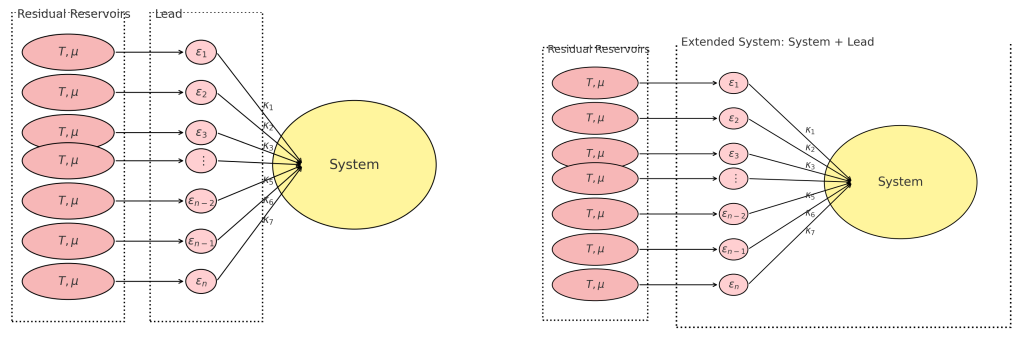
In this section we will discuss the aspects of the Mesoscopic lead construction shown in the above figure which is an example of the generalized reaction coordinate mapping where instead of dealing with infinite number of bath degrees of freedom we approximate the situation where we need to deal with only a finite number of bath modes which are called lead modes achieved by the Mesoscopic lead construction. Now, the number of lead modes required to bypass the problem with reasonably good approximation is a computational task. The idea is to get rid of the infinite number of bath modes and to work with finite degrees of freedom of the bath which will be computationally preferable. Here in the present context the bath is gain modified as we have done earlier in the case of the reaction coordinate mapping such that, the original bath after the mesoscopic lead construction consists of the lead which is a collection of finite number of bosonic or fermionic modes depending on the nature of the bath before the mapping and the finite number of residual reservoirs having infinite number of degree of freedom which are mutually non interacting and independent but they are individually connected to the lead modes which can be either bosonic or fermionic such that the mapping has to be exact. The above diagram shows the mesoscopic lead construction with only one bath but can be generalized for finite number of baths as well.

Let us consider the hamiltonian of the system coupled to a single bath before the mapping given by,

$$\begin{array}{c}\widehat{H}={\widehat{H}}_S+{\widehat{H}}_B+{\widehat{H}}_{SB}\end{array}$$

(510)

$$\begin{array}{c}{\widehat{H}}_B=\sum _{m=1}^{\infty }{\nu }_m{\widehat{d}}_m^{†}{\widehat{d}}_m\end{array}$$

(511)

$$\begin{array}{c}{\widehat{H}}_{SB}=\sum _{m=1}^{\infty }\left[{\kappa }_m{\widehat{S}}^{†}{\widehat{d}}_m+{\kappa }_m^{*}{\widehat{d}}_m^{†}\widehat{S}\right]\end{array}$$

(512)

Where, $\widehat{S}$ being any arbitrary non hermitian system operator and the interaction hamiltonian is written in the rotating wave approximation in general. The mesoscopic lead construction establishes the mapping between the two hamiltonians $\widehat{H}$ and ${\widehat{H}}_{\mathcal{M}}$ such that we can write the hamiltonian of the system after the mesoscopic lead construction as follows,

$$\begin{array}{c}{\widehat{H}}_{\mathcal{M}}={\widehat{H}}_{ext}+{\widehat{H}}_R+{\widehat{H}}_{LR}\end{array}$$

(513)

$$\begin{array}{c}{\widehat{H}}_{ext}={\widehat{H}}_S+{\widehat{H}}_L+{\widehat{H}}_{SL}\end{array}$$

(514)

$$\begin{array}{c}{\widehat{H}}_L=\sum _{m=1}^{L_B}{\omega }_m{\widehat{a}}_m^{†}{\widehat{a}}_m\end{array}$$

(515)

$$\begin{array}{c}{\widehat{H}}_{SL}=\sum _{m=1}^{L_B}\left[{\tilde{\kappa }}_m{\widehat{S}}^{†}{\widehat{a}}_m+{\tilde{\kappa }}_m^{*}{\widehat{a}}_m^{†}\widehat{S}\right]\end{array}$$

(516)

$$\begin{array}{c}{\widehat{H}}_R=\sum _{m=1}^{L_B}{\widehat{H}}_{R_m}=\sum _{r=1}^{\infty }\sum _{m=1}^{L_B}{\omega }_{rm}{\widehat{b}}_{rm}^{†}{\widehat{b}}_{rm}\end{array}$$

(517)

$$\begin{array}{c}{\widehat{H}}_{LR}=\sum _{r=1}^{\infty }\sum _{m=1}^{L_B}\left[{\xi }_{rm}{\widehat{a}}_m^{†}{\widehat{b}}_{rm}+{\xi }_{rm}^{*}{\widehat{b}}_{rm}^{†}{\widehat{a}}_m\right]\end{array}$$

(518)

$L_B$ denotes the number of the lead modes which is finite in this case. Now, the exactness condition of the mapping leads to the following,

$$\begin{array}{c}\sum _{m=1}^{\infty }\left[{\kappa }_m{\widehat{S}}^{†}{\widehat{d}}_m+{\kappa }_m^{*}{\widehat{d}}_m\widehat{S}\right]=\sum _{m=1}^{L_B}\left[{\tilde{\kappa }}_m{\widehat{S}}^{†}{\widehat{a}}_m+{\tilde{\kappa }}_m^{*}{\widehat{a}}_m^{†}\widehat{S}\right]\end{array}$$

(519)

$$\begin{array}{c}\sum _{m=1}^{\infty }{\kappa }_m{\widehat{d}}_m=\sum _{m=1}^{L_B}{\tilde{\kappa }}_m{\widehat{a}}_m,\sum _{m=1}^{\infty }{\kappa }_m^{*}{\widehat{d}}_m^{†}=\sum _{m=1}^{L_B}{\tilde{\kappa }}_m^{*}{\widehat{a}}_m^{†}\end{array}$$

(520)

Now, the requirement that the commutation (anti-commutation) relations for the bosonic (fermionic) case will remain intact before and after the mesoscopic lead construction such that with, ${\left[{\widehat{d}}_m,{\widehat{d}}_n\right]}_{\pm }=0={\left[{\widehat{d}}_m^{†},{\widehat{d}}_n^{†}\right]}_{\pm }\mathrm{and}{\left[{\widehat{d}}_m,{\widehat{d}}_n^{†}\right]}_{\pm }=\widehat{I}{\delta }_{mn}$ and ${\left[{\widehat{a}}_m,{\widehat{a}}_n\right]}_{\pm }=0={\left[{\widehat{a}}_m^{†},{\widehat{a}}_n^{†}\right]}_{\pm }$ and ${\left[{\widehat{a}}_m,{\widehat{a}}_n^{†}\right]}_{\pm }=\widehat{I}{\delta }_{mn}$ can directly write,

$$\sum _{m=1}^{\infty }|{\kappa }_m{|}^2=\sum _{m=1}^{L_B}{\left|{\tilde{\kappa }}_m\right|}^2$$

(521)

Where we have defined the general commutator (anti-commutator) bracket for any two arbitrary operators $\widehat{A}$ and $\widehat{B}$ as,

$${\left[\widehat{A},\widehat{B}\right]}_{\pm }=\widehat{A}\widehat{B}\pm \widehat{B}\widehat{A}$$

(522)

We note that, the mesoscopic lead construction is just an extended and general version of the reaction coordinate mapping belonging to the category of bosonic or fermionic particle mapping. Now similarly in the weak coupling limit the dynamics of the extended system can be described by the Redfield quantum master equation which is coupled to the residual reservoir. Along with that, if we assume that the coupling between the system and that of the mesoscopic lead is also weak then we can write the master equation for ${\widehat{\rho }}_{ext}\left(t\right)$ in Schrodinger picture as,

$$\begin{array}{c}{\displaystyle \frac{d{\widehat{\rho }}_{ext}\left(t\right)}{dt}}=i\left[{\widehat{\rho }}_{ext}\left(t\right),{\widehat{H}}_{ext}\right]+\sum _{m=1}^{L_B}{\gamma }_m{\overline{n}}_m\widehat{\mathcal{L}}\left[{\widehat{a}}_m^{†}\right]{\widehat{\rho }}_{ext}\left(t\right)+\sum _{m=1}^{L_B}{\gamma }_m\left(1+p{\overline{n}}_m\right)\widehat{\mathcal{L}}\left[{\widehat{a}}_m\right]{\widehat{\rho }}_{ext}\left(t\right)\end{array}$$

(523)

$$\begin{array}{c}\mathrm{with}\widehat{\mathcal{L}}\left[\widehat{c}\right]{\widehat{\rho }}_{ext}\left(t\right)=\widehat{c}{\widehat{\rho }}_{ext}\left(t\right){\widehat{c}}^{†}-{\displaystyle \frac{1}{2}}\left\{{\widehat{\rho }}_{ext}\left(t\right),{\widehat{c}}^{†}\widehat{c}\right\}\end{array}$$

(524)

Along with,

$$\begin{array}{c}\left[{\widehat{a}}_m{\widehat{a}}_n-p{\widehat{a}}_n{\widehat{a}}_m\right]=0=\left[{\widehat{a}}_m^{†}{\widehat{a}}_n^{†}-p{\widehat{a}}_n^{†}{\widehat{a}}_m^{†}\right]\end{array}$$

(525)

$$\begin{array}{c}\left[{\widehat{a}}_m{\widehat{a}}_n^{†}-p{\widehat{a}}_n^{†}{\widehat{a}}_m\right]=\widehat{I}{\delta }_{mn}\end{array}$$

(526)

$$\begin{array}{c}{\overline{n}}_m=\overline{n}({\omega }_m,T,\mu )\mathrm{with}\overline{n}(\omega ,T,\mu )={\displaystyle \frac{1}{e^{\beta (\omega -\mu )}-p}}\end{array}$$

(527)

We have defined ,

$$\begin{array}{c}{\gamma }_m=J_m\left({\omega }_m\right),J_m\left(\omega \right)=\sum _{r=1}^{\infty }\end{array}$$

(528)

The above equation is general for the bosons and fermions with, $p=\pm 1$ respectively.

3.3. Single Electron Transistor

The single electron transistor can be mathematically modeled by a single spinless quantum dot [5] connected to two different independent and non-interacting fermionic reservoirs and at the same time connected to a phonon bath which is bosonic in nature. All the three baths are independent and non-interacting such that the entire system can be described by the Hamiltonian of the following form,

$$\begin{array}{c}\widehat{H}={\widehat{H}}_S+{\widehat{H}}_{el}+{\widehat{H}}_{ph}+{\widehat{H}}_{S-el}+{\widehat{H}}_{S-ph}\end{array}$$

(529)

$$\begin{array}{c}{\widehat{H}}_S={\omega }_0{\widehat{d}}^{†}\widehat{d}\end{array}$$

(530)

$$\begin{array}{c}{\widehat{H}}_{el}=\sum _r\sum _m{\nu }_{rm}{\widehat{c}}_{rm}^{†}{\widehat{c}}_{rm}\end{array}$$

(531)

$$\begin{array}{c}{\widehat{H}}_{S-el}=\sum _r\sum _m\left[{\kappa }_{rm}{\widehat{d}}^{†}{\widehat{c}}_{rm}+{\kappa }_{rm}^{*}{\widehat{c}}_{rm}^{†}\widehat{d}\right]\end{array}$$

(532)

$$\begin{array}{c}{\widehat{H}}_{ph}={\displaystyle \frac{1}{2}}\sum _m\left[{\widehat{p}}_m^2+{\omega }_m^2{\widehat{x}}_m^2\right]\end{array}$$

(533)

$$\begin{array}{c}{\widehat{H}}_{S-ph}=-{\widehat{d}}^{†}\widehat{d}\sum _m{h}_m{\widehat{x}}_m+{\left({\widehat{d}}^{†}\widehat{d}\right)}^2\sum _m{\displaystyle \frac{h_m^2}{{\omega }_m^2}}\end{array}$$

(534)

The last term in ${\widehat{H}}_{S-ph}$ is essentially treated as the system renormalization term which is generally dropped while deriving the quantum master equation for the system but it can be absorbed in the hamiltonian of the system itself with,

$$\delta {\mathrm{\Omega }}_0^2=\sum _m{h}_m^2{\omega }_m^{-2}$$

(535)

Such that we can write,

$$\begin{array}{c}\widehat{H}={\widehat{H}}_S+{\widehat{H}}_{el}+{\widehat{H}}_{ph}+{\widehat{H}}_{S-el}\end{array}$$

(536)

$$\begin{array}{c}{\widehat{H}}_{ph}={\displaystyle \frac{1}{2}}\sum _m\left[{\widehat{p}}_m^2+{\omega }_m^2{\left({\widehat{x}}_m-{\displaystyle \frac{h_m}{{\omega }_m^2}}{\widehat{d}}^{†}\widehat{d}\right)}^2\right]\end{array}$$

(537)

$$\begin{array}{c}{\widehat{H}}_{el}=\sum _r\sum _m{\nu }_{rm}{\widehat{c}}_{rm}^{†}{\widehat{c}}_{rm}\end{array}$$

(538)

$$\begin{array}{c}{\widehat{H}}_{S-el}=\sum _r\sum _m\left[{\kappa }_{rm}{\widehat{d}}^{†}{\widehat{c}}_{rm}+{\kappa }_{rm}^{*}{\widehat{c}}_{rm}^{†}\widehat{d}\right]\end{array}$$

(539)

Now if we apply the reaction coordinate mapping for the phonon bath then after the reaction coordinate mapping the hamiltonian will become,

$$\begin{array}{c}\widehat{H}={\omega }_0{\widehat{d}}^{†}\widehat{d}+\sum _r\sum _m{\nu }_{rm}{\widehat{c}}_{rm}^{†}{\widehat{c}}_{rm}+\sum _r\sum _m\left[{\kappa }_{rm}{\widehat{d}}^{†}{\widehat{c}}_{rm}+{\kappa }_{rm}^{*}{\widehat{c}}_{rm}^{†}\widehat{d}\right]+{\displaystyle \frac{1}{2}}\left[{\widehat{P}}_1^2+{\mathrm{\Omega }}_1^2{\widehat{X}}_1^2\right]\end{array}$$

$$\begin{array}{c}+{\displaystyle \frac{1}{2}}\sum _{m\ne 1}\left[{\widehat{P}}_m^2+{\mathrm{\Omega }}_m^2{\widehat{X}}_m^2\right]-{\lambda }_0{\widehat{d}}^{†}\widehat{d}{\widehat{X}}_1-{\widehat{X}}_1\sum _m{C}_m{\widehat{X}}_m+{\displaystyle \frac{1}{2}}\sum _m{\displaystyle \frac{h_m^2}{{\omega }_m^2}}{\left({\widehat{d}}^{†}\widehat{d}\right)}^2\\ =\left({\omega }_0+{\displaystyle \frac{\delta {\mathrm{\Omega }}_0^2}{2}}\right){\widehat{d}}^{†}\widehat{d}+\sum _r\sum _m{\nu }_{rm}{\widehat{c}}_{rm}^{†}{\widehat{c}}_{rm}+\sum _r\sum _m\left[{\kappa }_{rm}{\widehat{d}}^{†}{\widehat{c}}_{rm}+{\kappa }_{rm}^{*}{\widehat{c}}_{rm}^{†}\widehat{d}\right]+{\displaystyle \frac{1}{2}}\left[{\widehat{P}}_1^2+{\mathrm{\Omega }}_1^2{\widehat{X}}_1^2\right]\end{array}$$

(540)

$$\begin{array}{c}+{\displaystyle \frac{1}{2}}\sum _{m\ne 1}\left[{\widehat{P}}_m^2+{\mathrm{\Omega }}_m^2{\widehat{X}}_m^2\right]-{\lambda }_0{\widehat{d}}^{†}\widehat{d}{\widehat{X}}_1-{\widehat{X}}_1\sum _m{C}_m{\widehat{X}}_m\end{array}$$

(541)

$$\begin{array}{c}={\widehat{H}}_{ext}^{\prime }+\sum _r\sum _m{\nu }_{rm}{\widehat{c}}_{rm}^{†}{\widehat{c}}_{rm}+\sum _r\sum _m\left[{\kappa }_{rm}{\widehat{d}}^{†}{\widehat{c}}_{rm}+{\kappa }_{rm}^{*}{\widehat{c}}_{rm}^{†}\widehat{d}\right]+{\displaystyle \frac{1}{2}}\sum _m\left[{\widehat{P}}_m^2+{\mathrm{\Omega }}_m^2{\widehat{X}}_m^2\right]-{\widehat{X}}_1\sum _m{C}_m{\widehat{X}}_m\end{array}$$

(542)

Where we have defined the extended system which comprises of the single spinless quantum dot coupled with the reaction coordinate such that,

$$\begin{array}{c}{\widehat{H}}_{ext}^{\prime }={\omega }_0^{\prime }{\widehat{d}}^{†}\widehat{d}+{\displaystyle \frac{1}{2}}\left[{\widehat{P}}_1^2+{\mathrm{\Omega }}_1^2{\widehat{X}}_1^2\right]-{\lambda }_0{\widehat{d}}^{†}\widehat{d}{\widehat{X}}_1\end{array}$$

(543)

$$\begin{array}{c}\mathrm{where}{\omega }_0^{\prime }={\omega }_0+{\displaystyle \frac{\delta {\mathrm{\Omega }}_0^2}{2}}\end{array}$$

(544)

Finally writing the operators ${\widehat{X}}_m$ and ${\widehat{P}}_m$ in terms of new pairs of bosonic creation and annihilation operators $\left({\widehat{a}}_m,{\widehat{a}}_m^{†}\right)$ such that with,

$$\begin{array}{c}{\widehat{X}}_m={\left({\displaystyle \frac{1}{2{\mathrm{\Omega }}_m}}\right)}^{{\displaystyle \frac{1}{2}}}\left[{\widehat{a}}_m+{\widehat{a}}_m^{†}\right],{\widehat{P}}_m=i{\left({\displaystyle \frac{{\mathrm{\Omega }}_m}{2}}\right)}^{{\displaystyle \frac{1}{2}}}\left[{\widehat{a}}_m^{†}-{\widehat{a}}_m\right]\end{array}$$

(545)

we can write,

$$\begin{array}{c}\widehat{H}={\widehat{H}}_{ext}^{\prime }+\sum _r\sum _m{\nu }_{rm}{\widehat{c}}_{rm}^{†}{\widehat{c}}_{rm}+\sum _r\sum _m\left[{\kappa }_{rm}{\widehat{d}}^{†}{\widehat{c}}_{rm}+{\kappa }_{rm}^{*}{\widehat{c}}_{rm}^{†}\widehat{d}\right]\end{array}$$

$$\begin{array}{c}+\sum _{m\ne 1}{\mathrm{\Omega }}_m{\widehat{a}}_m^{†}{\widehat{a}}_m-\left(\widehat{a}+{\widehat{a}}^{†}\right)\sum _m{H}_m\left({\widehat{a}}_m+{\widehat{a}}_m^{†}\right)\end{array}$$

(546)

$$\begin{array}{c}{\widehat{H}}_{ext}^{\prime }={\omega }_0^{\prime }{\widehat{d}}^{†}\widehat{d}+\mathrm{\Omega }{\widehat{a}}^{†}\widehat{a}-\lambda {\widehat{d}}^{†}\widehat{d}\left(\widehat{a}+{\widehat{a}}^{†}\right)\end{array}$$

(547)

$$\begin{array}{c}\widehat{H}={\widehat{H}}_{ext}^{\prime }+{\widehat{H}}_{el}+{\widehat{H}}_{S-el}+{\widehat{H}}_{ph}^{RE}+{\widehat{H}}_{RC-RE}\end{array}$$

(548)

$$\begin{array}{c}{\widehat{H}}_{ph}^{RE}=\sum _{m\ne 1}{\mathrm{\Omega }}_m{\widehat{a}}_m^{†}{\widehat{a}}_m,{\widehat{H}}_{RC-RE}=-\left(\widehat{a}+{\widehat{a}}^{†}\right)\sum _m{H}_m\left({\widehat{a}}_m+{\widehat{a}}_m^{†}\right)\end{array}$$

(549)

$$\begin{array}{c}{\widehat{H}}_{ext}^{\prime }={\omega }_0^{\prime }{\widehat{a}}^{†}\widehat{d}+{\widehat{H}}_{RC}+{\widehat{H}}_{S-RC}\end{array}$$

(550)

$$\begin{array}{c}{\widehat{H}}_{RC}=\mathrm{\Omega }{\widehat{a}}^{†}\widehat{a},{\widehat{H}}_{S-RC}=-\lambda {\widehat{d}}^{†}\widehat{d}\left(\widehat{a}+{\widehat{a}}^{†}\right)\end{array}$$

(551)

Where we have denoted the residual phonon bath hamiltonian by ${\widehat{H}}_{ph-RE}$ and ${\widehat{H}}_{RC-RE}$ describes the interaction of the reaction coordinate and the residual phonon bath hamiltonian. Where we have redefined the interaction coefficients respectively as, $\lambda ={\displaystyle \frac{{\lambda }_0}{\sqrt{\left(2\mathrm{\Omega }\right)}}}$ and $H_m={\displaystyle \frac{C_m}{\sqrt{4{\mathrm{\Omega }}_m\mathrm{\Omega }}}}$. We have also renamed ${\widehat{a}}_1\equiv \widehat{a}$ and ${\mathrm{\Omega }}_1\equiv \mathrm{\Omega }$ such that the frequency for the reaction coordinate is $\mathrm{\Omega }$. Just to mention that the exactness condition of the reaction coordinate mapping gives,

$${\widehat{d}}^{†}\widehat{d}\sum _m{h}_m{\widehat{x}}_m={\lambda }_0{\widehat{d}}^{†}\widehat{d}{\widehat{X}}_1\Rightarrow {\lambda }_0^2=\sum _m{h}_m^2$$

(552)

Along with the other conditions establishes before in the section of reaction coordinate mapping given by,

$$\begin{array}{c}{\mathrm{\Omega }}_{\alpha }^2{\delta }_{\alpha \beta }=\sum _m{\omega }_m^2{\mathrm{\Lambda }}_{\alpha m}{\mathrm{\Lambda }}_{\beta m}\end{array}$$

(553)

Now as we can see that due to the interaction between the quantum dot and the reaction coordinate the Hamiltonian of the extended system i.e ${\widehat{H}}_{ext}^{\prime }$ is not diagonal. So in order to diagonalize the Hamiltonian ${\widehat{H}}_{ext}^{\prime }$ we can use a specific unitary transformation called the Polaron transformation which diagonalizes the Hamiltonian ${\widehat{H}}_{ext}^{\prime }$. Let us define,

$$\widehat{U}=exp\left[{\displaystyle \frac{\lambda }{\mathrm{\Omega }}}{\widehat{d}}^{†}\widehat{d}\left(\widehat{a}-{\widehat{a}}^{†}\right)\right]$$

(554)

such that it satisfies the unitarity condition i.e. ${\widehat{U}}^{†}\widehat{U}=\widehat{I}$ which can be readily understood from the fact that the fermionic creation and annihilation operators commutes with the corresponding bosonic counterparts. Then with the unitary transformation of ${\widehat{H}}_{ext}^{\prime }$ with $\widehat{U}$ it can be made diagonal such that,

$$\begin{array}{c}{\widehat{H}}_{ext}^D=\widehat{U}{\widehat{H}}_{ext}^{\prime }{\widehat{U}}^{†}\end{array}$$

(555)

$$\begin{array}{c}\widehat{U}{\widehat{H}}_{ext}^{\prime }{\widehat{U}}^{†}=\widehat{U}{\widehat{H}}_S{\widehat{U}}^{†}+\widehat{U}{\widehat{H}}_{RC}{\widehat{U}}^{†}+\widehat{U}{\widehat{H}}_{S-RC}{\widehat{U}}^{†}\end{array}$$

(556)

$$\begin{array}{c}\widehat{U}{\widehat{H}}_S{\widehat{U}}^{†}={\omega }_0^{\prime }{\widehat{d}}^{†}\widehat{d}\end{array}$$

(557)

$$\begin{array}{c}\widehat{U}{\widehat{H}}_{RC}{\widehat{U}}^{†}=\mathrm{\Omega }\widehat{U}{\widehat{a}}^{†}{\widehat{U}}^{†}\widehat{U}{\widehat{a}}^{†}{\widehat{U}}^{†}=\mathrm{\Omega }\left[\widehat{a}+{\displaystyle \frac{\lambda }{\mathrm{\Omega }}}{\widehat{d}}^{†}\widehat{d}\right]\left[{\widehat{a}}^{†}+{\displaystyle \frac{\lambda }{\mathrm{\Omega }}}{\widehat{d}}^{†}\widehat{d}\right]\end{array}$$

(558)

$$\begin{array}{c}\widehat{U}{\widehat{H}}_{S-RC}{\widehat{U}}^{†}=-\lambda {\widehat{d}}^{†}\widehat{d}\left[\widehat{a}+{\widehat{a}}^{†}+{\displaystyle \frac{2\lambda }{\mathrm{\Omega }}}{\widehat{d}}^{†}\widehat{d}\right]\end{array}$$

(559)

$$\begin{array}{c}\widehat{U}{\widehat{H}}_{ext}^{\prime }{\widehat{U}}^{†}={\omega }_0^{\prime }{\widehat{d}}^{†}\widehat{d}+\mathrm{\Omega }{\widehat{a}}^{†}\widehat{a}-{\displaystyle \frac{{\lambda }^2}{\mathrm{\Omega }}}{\widehat{d}}^{†}\widehat{d}={\overline{\omega }}_0{\widehat{d}}^{†}\widehat{d}+\mathrm{\Omega }{\widehat{a}}^{†}\widehat{a}\end{array}$$

(560)

Where we have introduced the redefined quantum dot frequency denoted by, ${\overline{\omega }}_0$ defined as,

$${\overline{\omega }}_0={\omega }_0^{\prime }-{\displaystyle \frac{{\lambda }^2}{\mathrm{\Omega }}}={\omega }_0-{\displaystyle \frac{1}{2}}\sum _m{\displaystyle \frac{h_m^2}{{\omega }_m^2}}-{\displaystyle \frac{{\lambda }^2}{\mathrm{\Omega }}}$$

(561)

And we have used the B.H.C equality such that with,

$$e^{\widehat{A}}\widehat{B}{e}^{-\widehat{A}}=\widehat{B}+\left[\widehat{A},\widehat{B}\right]+{\displaystyle \frac{1}{2!}}\left[\widehat{A},\left[\widehat{A},\widehat{B}\right]\right]+...$$

(562)

Now with, $\widehat{A}={\displaystyle \frac{\lambda }{\mathrm{\Omega }}}{\widehat{d}}^{†}\widehat{d}\left(\widehat{a}-{\widehat{a}}^{†}\right)$ and $\widehat{B}={\widehat{a}}^{†}$ we get, $\left[\widehat{A},\widehat{B}\right]={\displaystyle \frac{\lambda }{\mathrm{\Omega }}}{\widehat{d}}^{†}\widehat{d}$ such that due to the commutation of the fermionic operators with the bosonic operators we can write $\left[\widehat{A},\left[\widehat{A},\widehat{B}\right]\right]=0$ such that, we can directly write,

$$\begin{array}{c}\widehat{U}{\widehat{a}}^{†}{\widehat{U}}^{†}={\widehat{a}}^{†}+{\displaystyle \frac{\lambda }{\mathrm{\Omega }}}{\widehat{d}}^{†}\widehat{d}\end{array}$$

(563)

$$\begin{array}{c}\widehat{U}\widehat{a}{\widehat{U}}^{†}=\widehat{a}+{\displaystyle \frac{\lambda }{\mathrm{\Omega }}}{\widehat{d}}^{†}\widehat{d}\end{array}$$

(564)

Such that the diagonalized Hamiltonian of the Extended system obtained after the Reaction Coordinate polaron Transformation is given as,

$${\widehat{H}}_{ext}^D={\overline{\omega }}_0{\widehat{d}}^{†}\widehat{d}+\mathrm{\Omega }{\widehat{a}}^{†}\widehat{a}$$

(565)

As we can see that ${\widehat{H}}_{ext}^D$ is just the sum of the hamiltonians of the quantum dot with a modified frequency ${\overline{\omega }}_0$ and the Hamiltonian of the reaction coordinate such that the energy spectrum of the diagonalised hamiltonian is readily obtained. As ${\widehat{H}}_{ext}^D$ is separable and can be written as the sum of the micro-hamiltonians of the quantum dot and the reaction coordinate then the energy eigenvalues will be the sum of the energy eigenvalues of the quantum dot and that of the reaction coordinate which is equivalent to a 1D harmonic oscillator, such that due to the fact that, ${\left({\widehat{d}}^{†}\widehat{d}\right)}^2={\widehat{d}}^{†}\widehat{d}$ i.e. the fermionic number operator is idempotent then it can have only eigenvalues 0 and 1 respectively and the eigenvalues of the reaction coordinate Hamiltonian will be $n\mathrm{\Omega }$ apart from the zero point energy term. Such that the energy eigenvalues of ${\widehat{H}}_{ext}^D$ will be,

$$E_n^{ext}={\overline{\omega }}_{0}p+n\mathrm{\Omega }$$

(566)

where, p can be either 0 or, 1 and n goes from $0,1,..,\infty$.