
Submitted:
14 November 2025
Posted:
18 November 2025
You are already at the latest version
Abstract
A computational fluid dynamics analysis of the anode side of a proton exchange membrane (PEM) electrolyzer cell has been conducted. The geometry is symmetrical and allows for the investigation of a single feed channel and a single exhaust channel in an interdigitated flow field. The model utilizes the Eulerian approach and thus solves a full set of conservation equations for both gas and liquid phase. Moreover, it is non-isothermal and it includes phase change of water. The operating stoichiometric flow ratio results in segregated flow in the horizontal flow channels. At a current density of 1.0 A/cm2, a local hot spot with a temperature increase of 7 °C is predicted. A reduction in the operating pressure below atmospheric pressure results in a more favorable concentration ratio of water vapor to oxygen at the PTL/CL interface, and the temperature distribution is more even. However, when the outlet pressure is too low, the outlet temperature is below the inlet temperature which makes this operation mode unfeasible. Adjustment of the back pressure can generally be used to control the temperature of the electrolyzer.
Keywords:
PEM electrolyzer
; Euler-Euler model
; segregated channel flow
; computational fluid dynamics
; electrolyzer operating conditions
; interdigitated flow field
1. Introduction
In recent years, there has been a growing interest in generating hydrogen via water electrolysis in order to store intermittent energy sources like solar and wind in chemical form. Among the different types of water electrolyzers, proton exchange membrane (PEM) water electrolyzers have the advantage of quick start-up times, very pure hydrogen generation, and an operating temperature of around 80 °C which makes them suitable to couple to a district heating grid. Importantly, it is possible to generate hydrogen at a pressure of several hundred bars which eliminates the need of a costly and service-intensive compressor. The main disadvantage of this technology is the need of precious metal catalysts such as iridium and platinum which leads to high capital expenditures [1]. Therefore, reducing the catalyst loading and replacing the precious metals is nowadays one of the prime research objectives. The efficiency of PEM electrolyzers is in the range of above 70%, ideally above 80%, so that the operating expenses are moderate [2]. A comparison of the different electrolyzer types was given by Schmidt et al. [1]. On balance, if PEM electrolyzers can operate at the storage pressure, and the amount of catalyst can be reduced, then this technology can be the choice for small and intermediate scale operations.
The half-cell and full cell reactions in a PEM electrolyzer are:
A schematic of a PEM electrolyzer is shown in Figure 1. Water is fed to the anode side where it is split up into electrons, protons and oxygen. The protons migrate through the membrane, most likely in the form of hydronium ions, and recombine at the cathode side to form hydrogen.
The heat and mass transfer processes inside the electrolyzer, especially inside the anode compartment where the expensive iridium-based catalyst is used, are complex. Clearly, a fundamental understanding of the multiphase flow phenomena can lead to improved performance and reduced catalyst loading.
In the past, computational fluid dynamics (CFD) analysis of a PEM electrolyzers were conducted in order to shed light into the distribution of water, oxygen and the temperature in an operating electrolyzer. Grigoriev et al. [3] were among the first to show the water distribution in their GenHy® 1000 PEM electrolyzer stack, calculated with COMSOL Multiphysics. However, details of their model were not disclosed.
In 2011, Nie and Chen [4] applied Fluent v6.3 to study multiphase flow in the anode side of a PEM electrolyzer. These authors employed a mixture model, meaning that one set of Navier-Stokes equations was solved for both phases, and applied an algebraic slip velocity depending on the local Reynolds number. The water flow rate was fixed, and the oxygen flow rate was varied. The flow field geometry investigated was a square with straight channels.
Olesen et al. [5] modelled the water and oxygen distribution in the anode flow field plate of the Primolyzer® design by the Danish manufacturer IRD A/S. They used the Eulerian approach where a set of transport equation is solved for each phase. Their nonisothermal results indicated that flow maldistribution can lead to temperature discrepancies of up to 8 °C which will limit the nominal operating temperate to around 80 °C due to material restrictions of the Nafion membrane. The modelling tool was the commercial software Ansys CFX Version 12.0 (ANSYS Inc.). Later on, Lafmejani et al. [6] employed the Volume of Fluid approach implemented in Ansys Fluent Version 16.0 (ANSYS Inc.) to study the multiphase flow in an expanded cathode flow field.
Zinser et al. [7] studied mass transport in a anodic porous transport layer (A-PTL) in PEM water electrolysis, identifying regions of dry-out where the electrolyzer can not function. Their model was self-developed and coded in MATLAB. In addition, they experimentally determined material properties of a Ti sintered fibre porous transport layer (PTL).
In 2020, Upadhyay et al. [8] employed Ansys Fluent to simulate the flow through a round anode flow field plate. The model was transient and single phase, and the flow was entering from one side of the bipolar plate and leaving on the other side, as e.g. in the electrolyzer design by Millet et al. [9] or the Primolyzer® design modeled by Olesen et al. [5]. Later on, Upadhyay et al. [10] employed the Ansys Fluent 2020R2 module to study different channel configurations in a straight channel flow field. The model was single phase and ignored the effect of gravity, but the comparison with experimental performance data was very good.
Recently, a review of the different modelling approaches has been given by Falcão and Pinto [11]. Lastly, Su et al. [12] published a CFD study of different rectangular flow field geometries.
Overall, the number of studies that entailed CFD are few compared to PEM fuel cells, and the fewest employ a multiphase solver, counting the commercial ANSYS Fluent module as single phase. Moreover, buoyancy effects in modelling have often been ignored, although they are of particular importance in electrolyzer design which is why alkaline electrolyzers are usually horizontally oriented cylinders.
In this work, a multi-fluid approach is applied in order to model the liquid water, water vapor and oxygen distribution under different operating conditions. The investigated flow field has been designed at Aalborg University, and it is shown in Figure 2. In this electrolyzer design, the plates are oriented horizontally which is different from most other designs. The preferred orientation of the plates is currently subject of investigation.
The anode side flow channels for the water and oxygen are radial, where the water enters from the center hole and the multiphase flow leaves at the outside. This figure suggests that the anode channels face upward and are placed below the porous medium, forcing the water through it. The cathode channels are spiral, and the hydrogen escape hole is shown on the right in Figure 2. The electrolyzer stack is placed in a vessel so that the oxygen and water mixture is diverted to the bottom where a heat exchanger/recuperator is located. The phases are separated, and the water is recirculated while saturated oxygen leaves from a separate hole. Full details of the electrolyzer design can be found in reference [13].
The goal of the current work is to gain basic understanding of the multiphase flow at the anode side of this electrolyzer, especially in terms of the effect of gravity and the length of the anode inlet and outlet channels. In addition, an improved fundamental understanding of the thermal management of PEM electrolyzers is needed to attain higher current densities. It was shown by Olesen et al. [5] that the amount of waste heat increases nonlinearly with current density, and therefore, proper thermal management is imperative to attain high current densities. In order to obtain an improved understanding, a multi-fluid model was developed in the software CFX-4.4, a formerly commercial CFD package that employs an IJK-structured grid and has strong multiphase flow modelling capacities.
2. Model Description
2.1. Assumptions
The following assumptions and simplifications are made in this model:
- The problem is steady state.
- The flow is laminar.
- The gas phase is an ideal gas.
- The liquid phase contains only water.
- The porous medium is isotropic.
- In the channel, the flow is segregated and in the Stokes regime.
- The catalyst layer is a thin interface and its thickness ignored.
The fact that the model is steady state essentially rules out inherently transient flow phenomena such as slug flow, where larger gas bubbles are periodically driven out of the channel when the pressure gradient is sufficiently high. It will be shown that the operating conditions investigated lead to wavy-stratified flow and even slug flow, where the first may still be captured with a steady state model, but the latter may not. The implications of this will be discussed below.
The last assumption was also made by Olesen et al. [5]. The channel length investigated here is in the order of 50 mm while the CL thickness is in the order of 10 microns. It was found in prior work by Marshall et al. [14], and Millet et al. [15] that the electrolyzer performance depends strongly on the type of catalyst used, but in the current study the operating current and voltage are taken as input parameters, and the output is the multiphase behavior and the thermal management under the conditions investigated. From this, learnings can be gathered as to how to improve the bipolar plate design and the cell performance.
2.2. Modelling Domain and Computational Grid
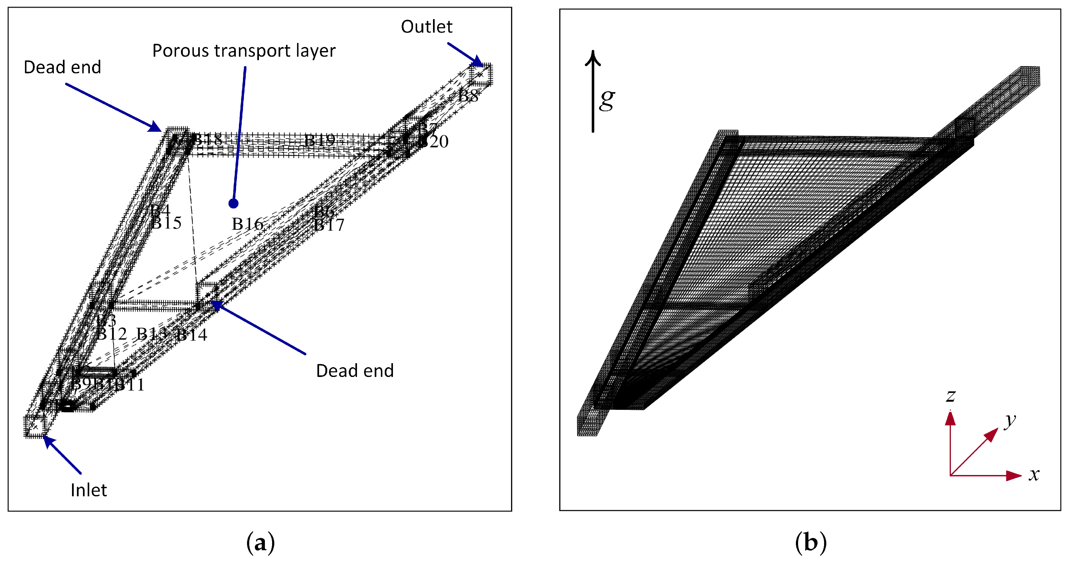
The model geometry and the computational grid are shown in Figure 3. The anode side flow field consists of straight channels where the water is fed from a central hole and is flowing radially outward. The flow field is interdigitated which means that the water is forced through the porous transport layer. In the case presented here, the plates are actually turned around compared to Figure 2, meaning that the anode flow channels are placed below the porous medium and the water is forced to flow upward. Both plate orientations were studied, and the upward facing channels seem to provide a better solution that will be discussed in detail below.
The mesh consists of a total of 20 Blocks, where Blocks 1-4 constitute the feed channel with the inlet where a velocity condition for the liquid water is applied and blocks 5-8 constitute the escape channel with the outlet. In the first hardware design, shown in Figure 2, the escape channels started close to the center of the plate [13]. The effect of the channel length is subject of future investigation. Blocks 9-20 constitute the porous transport layer which is around 200 microns thick. The total number of cells is 63,000, and they are all hexahedral. Because the cell section investigated is small, just 7.5 degrees, a cartesian grid was used rather than a cylindrical grid. The cell layer in the bottom represents the catalyst layer where the water vapor is consumed and oxygen is being produced. This means the CL is assumed to be a thin interface.
As mentioned, the active area of the investigated domain is a section of 7.5 °, where the active area stretches in a channel length from 10 mm to 50 mm. With this, the active area investigated is:
2.3. Model Equations
The model employs the Euler-Euler approach where two full sets of conservation equations are solved to model the transport in the gas phase and liquid phase.
The continuity equation is:
where is the porosity of a porous medium, the subscript represents different phases, and r stands for the volume fraction. In the region of the channels, the porosity is set to one. Furthermore, is the density, is the velocity vector , S denotes source terms, for example due to the electrochemical reaction at the catalyst layer. The last bracket denotes mass exchange between phases due to phase change.
Likewise, the momentum equations are:
where P is the pressure which is assumed to be the same for both phases, and Bα is the so-called body-force term. The third term on the right hand side accounts for interfacial drag, and the last term for momentum exchange due to phase change of species. These terms will be explained in detail below. The first term on the right hand side accounts for gravity, and in these simulations it was found to be of great importance.
The stress tensor for a Newtonian fluid is:
where is the dynamic viscosity of phase .
In addition to the Navier-Stokes equations that calculate the pressure distribution and the two-phase velocity fields, one species transport equation is solved for. It is most convenient to track the species that is undergoing phase change, in this case the water. Thus, a transport equation for water vapor is accounted for, while the background fluid in the gas phase is the oxygen.
where indicates the mass fraction of water vapour and is the binary diffusion coefficient of water vapour in air, specified below.
The system of equations is closed by the ideal gas law:
where W is the molecular weight of air (28.84 g/mol) and R is the universal gas constant. For the liquid phase, the density is taken to be constant.
Finally, the energy equation is solved for to calculate the temperature distribution.
where H is the total enthalpy, given in terms of static (thermodynamic) enthalpy h by:
2.4. Source Term Implementation
The above conservation equations include various source terms that are important to define in user subroutines provided by CFX-4. The detailed implementation will be defined next.
2.4.1. Calculation of the Local Current Density
At the lowest cell in the z-direction, where the interface between the porous GDL and the catalyst layer is located, there is production of oxygen in the gas phase. This must be accounted for by a source term that is applied to the gas phase continuity equation, equation 5, simply by:
In this model, oxygen is considered the background species in the gas phase, and the transport equation of water vapour is solved. Likewise, there is a sink term for water vapor which is accounted for in the species transport equation, the continuity equation and the volume fraction equation:
For the determination of the local current density, the average concentration of water vapor in the lowest computational cell of the domain (low-z), where the GDL/CL interface is located, is used to determine the local current density:
2.4.2. Implementation of Porous Media Resistance
The body force is written as:
where and are the to be specified parameters, and they can be used to approximate the phenomenological Darcy equation [16,17]. Written in terms of the advection velocity U, Darcy’s law for flow in the x-direction reads:
where K is the hydraulic permeability in (). Thus, reformulation yields:
so that
which are the specified body-force terms in the porous media. For the specification of the relative permeabilities, a cubical form is chosen:
where s is the liquid saturation, equal to the liquid phase volume fraction .
2.4.3. Implementation of Drag Terms
The second term on the right-and side in equation 7 is used to specify the drag term in the flow channels. In order to determine the correct drag coefficients, the flow regime has to be identified first. To this end, the well-known modified Baker diagram has been consulted [18,19], shown in Figure 4. Here, the G values represent mass fluxes with for air and for water.
In the current cases, the liquid flow rate is constant to represent a stoichiometry of =350 at a current density of i=1.0 A/cm2. Thus, the liquid flux is:
The liquid flow rate has been kept constant in these simulations and the amount of water that evaporates is small. For a current density of i=1.0 A/cm3, the oxygen flux is at the outlet is:
This places all likely operating points into the stratified flow regime, but close to the plug/slug flow regime in the Baker diagram. A more detailed calculation using the complex chart by Taitel and Dukler [20] places the flow regimes investigated in between the wavy stratified and the slug flow regime. By comparison, the flow field plates investigated by Olesen et al. [5] were of very similar size as the ones investigated here, but because they are oriented vertically, the flow regime was slug/plug flow. The quick analysis above only included the oxygen flow in the gas phase, while the addition of water vapor moves the flow regime even closer to the unsteady slug flow.
In fact, it was observed in the calculations that the water mass flow and the pressure in the outlet channel was slightly pulsating, i.e. in the steady-state solution, the outlet flow showed a slight oscillating behavior with iterations when it was fully converged. But it was also observed that the key results investigated here such as the oxygen and water vapor concentration near the catalyst and the temperature distribution did not vary for the converged solution, i.e. the flow in the outlet channel was decoupled from what occurred in the PTL. This can be expected when the pressure drop over the PTL is much higher than the pressure drop along the outlet channel. This observation gives confidence in the CFD results as it predicts slug/plug flow when it should, and the key results can still be interpreted as they are independent of the flow pattern in the outlet channel.
Having thus established that the flow is expected in the stratified flow or slug flow regime, the drag coefficients can be determined. These are the coefficients in the momentum equation as well as the interphase transfer coefficient in the energy and species equation for water vapor. According to the CFX-4.4 subroutine USRIPT, for laminar, stratified flow the drag coefficient can be specified as:
where
in the Stokes flow regime. Re is the Reynolds number, defined as:
where is the slip velocity between both phases. The mixture density is calculated out of the phasic volumes:
where is again the volume fraction of phase i in each computational volume. Combining the above yields for the drag coefficient:
where, according to the Isbin equation, the mixture viscosity is calculated in a similar way as the mixture density, and
where and is the length scale, here taken to be 1 mm. Finally, the interfacial area is calculated from:
Here, is the physical volume of each control volume and is the interface length scale, here also taken to be 1 mm. With this, the drag coefficient in the momentum equation is defined, and it will be seen in the results that the channel flow is segregated, as intended.
2.4.4. Implementation of Phase Change
The amount of mass undergoing phase change, is either water vapor condensing from the gas phase into the liquid phase or evaporation from the liquid phase into the gas phase. In the current implementation, the source term for oxygen production in the catalyst layer is in the gas phase conservation equation, while pure liquid water enters the electrolyzer. The created gas phase volume leads to evaporation of water, written as [16,21]:
where is the convective mass transfer coefficient and is the interfacial area, both described below. is the molecular weight of water and is the partial pressure of water vapor inside an given control volume. The saturation pressure corresponds to the temperature calculated in the respective control volume, and the relationship is described via Antoine’s equation:
where A = 23.196, B = 3816.44, C = -46.13, and T is the temperature in [K]. The resulting pressure is then in [Pa].
Similar to Olesen et al. [22,23], in case of condensation, the convective mass transfer coefficient in the porous region is calculated out of the mean molecular speed :
where is a dimensionless uptake coefficient which was estimated to be 0.006 [22], is the mean molecular gas speed, and is the mixture molecular weight. With this, the unit for is [m/s].
In case of evaporation, the convective mass transfer coefficient is calculated via:
Here, is the mixture concentration in [mol/m3]:
where is the universal gas constant (8.314J/mol-K). For the binary diffusion coefficient , the relation for water vapor in air was used [24]:
where is the total pressure in [atm] and T is the temperature in [K]. Finally, the Sherwood number Shm is given by:
where the Reynolds number is again based on the slip velocity between the phases:
The slip velocity is calculated out of the relative velocity components:
Where i denotes the three different directions x, y, and z. The slip velocity is then:
The characteristic pore diameter is described below, and the Schmidt number Sc is defined as:
The specific interfacial area is calculated out of the liquid volume fraction, assuming the liquid body is split up into droplets that fill the pores with an average radius corresponding to the characteristic radius :
For a dry permeability of k = and a porosity of , this results in a characteristic pore diameter of around 10 microns. Grigoriev et al. [25] determined such properties for various different PTL types, and the characteristic pore size was in this order of magnitude.
The pore size was then used to calculate the interfacial area . In the porous media, the volume fraction of the liquid phase in each control volume was divided into assumed droplets that occupied pores with the characteristic pore size [16]. The number of droplets in a given control volume is thus:
and the interfacial area is then calculated according to:
where care must be taken that is by naming convention the dimensionless volume fraction of the liquid phase whereas is the characteristic radius [m].
It can, however, happen that the liquid volume fraction becomes so large that the interfacial area decreases again. Therefore, the same procedure was carried out for the gas phase occupying the pores, and the interfacial area was set to be the minimum of the two. Combining all of the above yields the mass transfer rate per computational cell in [kg/s]. The results show that the gas phase was at an average relative humidity between 99% and 100% wherever liquid phase is present.
Finally, in order to determine the mass transfer in the flow channels, the Reynolds analogy is employed so that it holds:
where L is a characteristic length scale. The thus calculated convective mass transfer coefficient:
has the units [m/s] and is therefore equivalent to .
2.4.5. Energy Equation
The source term in the energy equation, , accounts for the waste heat generation due to the electrochemical reaction as well as the cooling or heating due to the phase change of water. As the water enters the electrolyzer in the liquid phase and the oxygen is produced in the gas phase, there is water evaporating into the gas. This happens predominantly inside the porous media, and it leads to a cooling effect.
Inside the CL, the waste heat is generated, depending on the local current density that was calculated out of the local water vapor concentration. To this end, an electrolyzer voltage of 1.85 V at the specified current density was assumed, taken from Olesen et al. [5]. It is well known that the performance depends strongly on the type and the loading of the catalyst, and therefore it was not attempted to model the performance at this stage.
The heating term at the lower PTL interface where the CL is located is [5]:
Assuming a cell voltage as V and using = 241,820 J/mole when the water is consumed in the form of vapor [26], this yields a total heat source of 0.94 W for the active area of 1.57 cm2 investigated here. The corresponding electrical efficiency is 1.482 V/1.85 V= 80%, and the total power in this section is 2.9 W.
2.5. Boundary Conditions
At the inlet, the velocity and temperature of the incoming water are specified. The velocity is calculated out of the stoichiometric flow ratio of and the current density of 1.0 A/cm2. The temperature was equal to the operating temperature of 80 °C. For the pressure, zero gradient was assumed.
At the outlet, the absolute pressure of 1 atm was applied for the base case, and zero gradient conditions were used for all other transport equations.
The inlet and outlet are located at the low-x and the high-x interfaces. At low-y and the high-y interfaces (left and right in Figure 3 a), symmetry conditions are applied so that only half a channel width needed to be modeled. At all other outer boundaries, wall boundary conditions are applied which prevent any species or heat fluxes.
2.6. Material Properties
Main input parameters for the model were the material properties of the PTL. These are standard values, although the tortuosity was chosen somewhat higher than the usual value around . For the PTL, various materials can be used from carbon fiber paper which is said to lead to carbon corrosion to sintered titanium powder which will have a higher thermal conductivity. The results discussed are only mildly affected by these values. With the permeability and the porosity given, the characteristic power size can be calculated according to Equation 42.

Table 1.
Key material properties.
| Property | Symbol | Unit | Value |
|---|---|---|---|
| Porosity | [-] | 0.75 | |
| Tortuosity | [-] | 5 | |
| Hydraulic Permeability | K | [m2] | 2 |
| Thermal Conductivity | [W/m-K] | 5.0 |
2.7. Solution Procedure
The calculations presented here were challenging, and a solution procedure had to be developed to by and by switch on the different terms.
- Run the case with liquid water only, where water is running through the geometry at a prescribed combination of current density and stoichiometry. This is similar to experiments where first water is run through the stack without drawing current, and then the current density is step-wise increased, keeping the flow rate constant.
- Switch on the oxygen source term where the current density is uniform. The thus obtained results already yield useful insights in the gas-liquid distribution.
- Switch on phase change of water. This is of interest in order to better understand, to which degree the gas phase is saturated with vapor, and eventually to determine the concentration ratio between oxygen and water vapor. However, only mass transfer is considered, not yet the energy terms.
- Adjust the local current density to account for the water vapor distribution and switch on the sink ter for water vapor.
- Switch on the sink and source terms in the energy equation to obtain the temperature distribution.
2.8. Numerical Procedure
It was found that the algebraic multigrid (AMG) solver, while taking more time per iteration, resulted in the most robust convergence. Moreover, the AMG solver is known for producing a nearly grid independent solution, especially seeing that there are no items in the geometry that can only be accounted for by a finer mesh.
The PISO algorithm was employed for the pressure velocity coupling. For all transport equations, a combination of under-relaxation factors and false time steps were used. Note that for all these values, default values are automatically specified in CFX-4.4.
3. Results
The Results section is divided into two parts: a detailed presentation of the base case results and a parametric study section where the operating pressure of the electrolyzer was stepwise reduced from 1 bar to 0.5 bar. The plate orientation was such that the channels are facing upward and the water is pressed through the porous medium from below.
3.1. Base Case Results
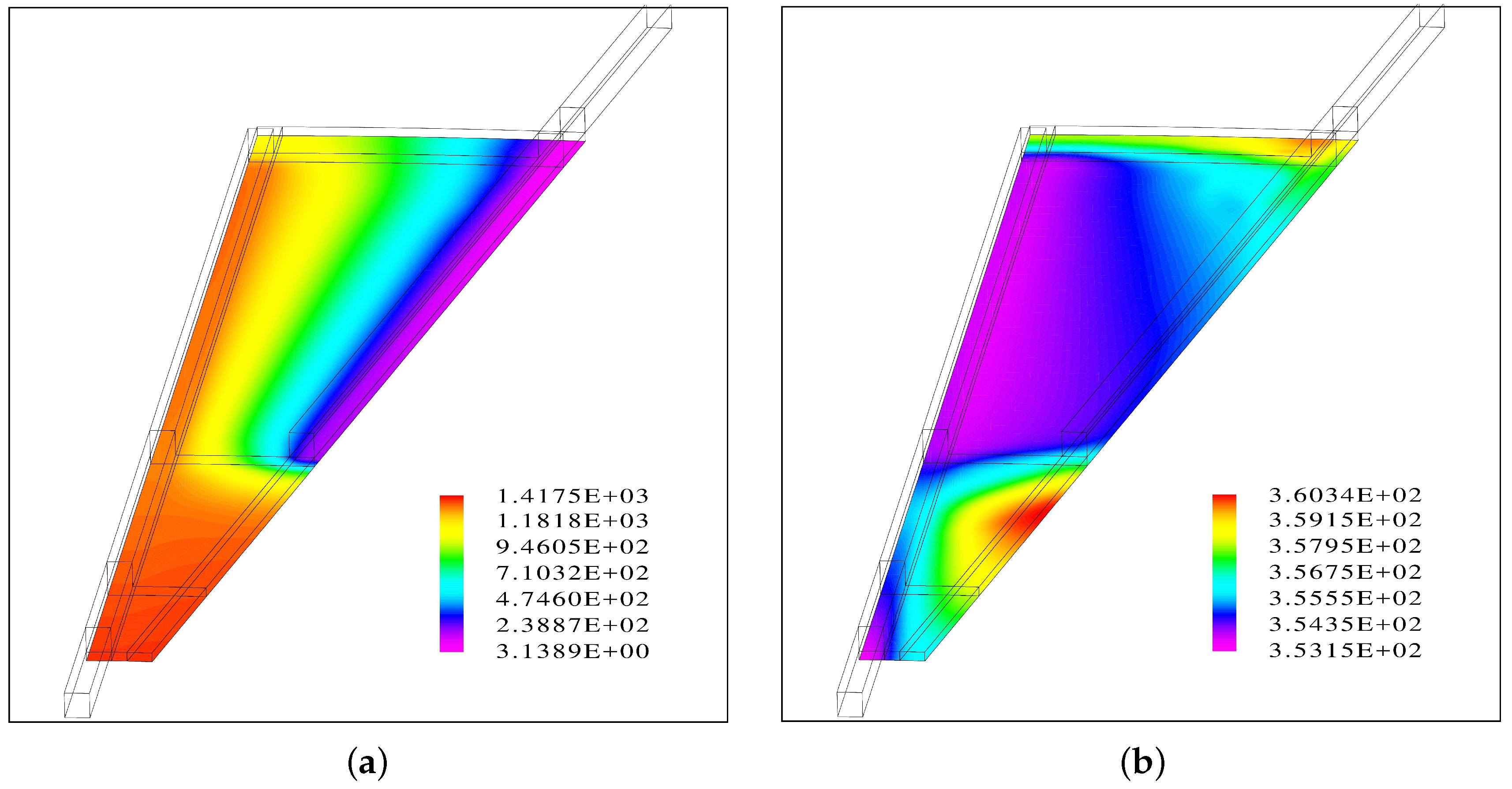
The base case was calculated for ambient pressure at the anode outlet. The resulting relative pressure distribution at the low-z interface where the electrochemical reaction occurs is shown in Figure 5 a). The relative pressure is equal to zero at the outlet, and the calculated relative pressure at the inlet is around 1418 Pa. Across the porous medium, there is a smooth drop-off in pressure, and the value is nearly constant underneath the channels. Such a smooth and intuitive distribution gives confidence in the overall results.
The calculated temperature distribution in the same layer is shown in Figure 5 b). The nominal cell temperature is 80 °C, hence 353.15 K, and there is a predicted peak temperature increase of 7 °C which can be found before the outlet channel section begins and at the outer edge near the outlet channel. This means that both hot spots are predicted in regions where either the outlet channel has not yet started or the inlet section has ended, and the region between the two channels experiences only a mild temperature increase of 3 °C. This could be important for the placing of catalyst and it deserves further investigation. The outlet channel begins some distance from the inner radius, and this as done to avoid short-circuiting the water, but if this leads to a hot spot, the outlet channel should begin closer to the center. The reason for the existence of the hot spot is that there is a predicted gas bubble here with no liquid phase present, as will be shown below. By contrast, the region between two channels is predicted in the multiphase regime, and the evaporative cooling prevents hot spots, as will also be seen below.
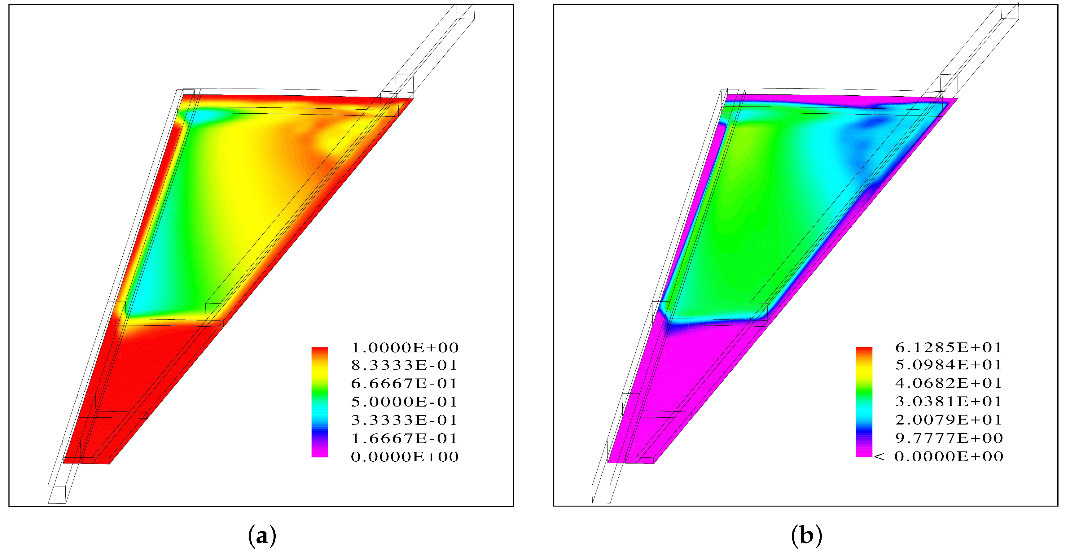
The distribution of the gas phase volume fraction and the local evaporation rate is shown in Figure 6. By definition, positive values indicate evaporation and negative values condensation. As was mentioned above, there is a region with gas phase only at the inner part of the cell before the outlet channel starts. This coincides with the region of the inner hot spot. Moreover, all-dry regions are predicted underneath the channels and near the outer edge where the other hot region is located. These are also the regions in the cell where the evaporation rate is zero while evaporation is highest between the two channels and nearer to the inlet channel, where the temperature was predicted to stay constant. It appears desirable to operate an electrolyzer isothermally, and it is obvious that this local evaporation supports that. From these figures, it is concluded that the region between the channel is favored and should be as large as possible, i.e. the radius of the plates can be larger and both inlet and outlet channel should be as long as possible. However, further investigation is needed.
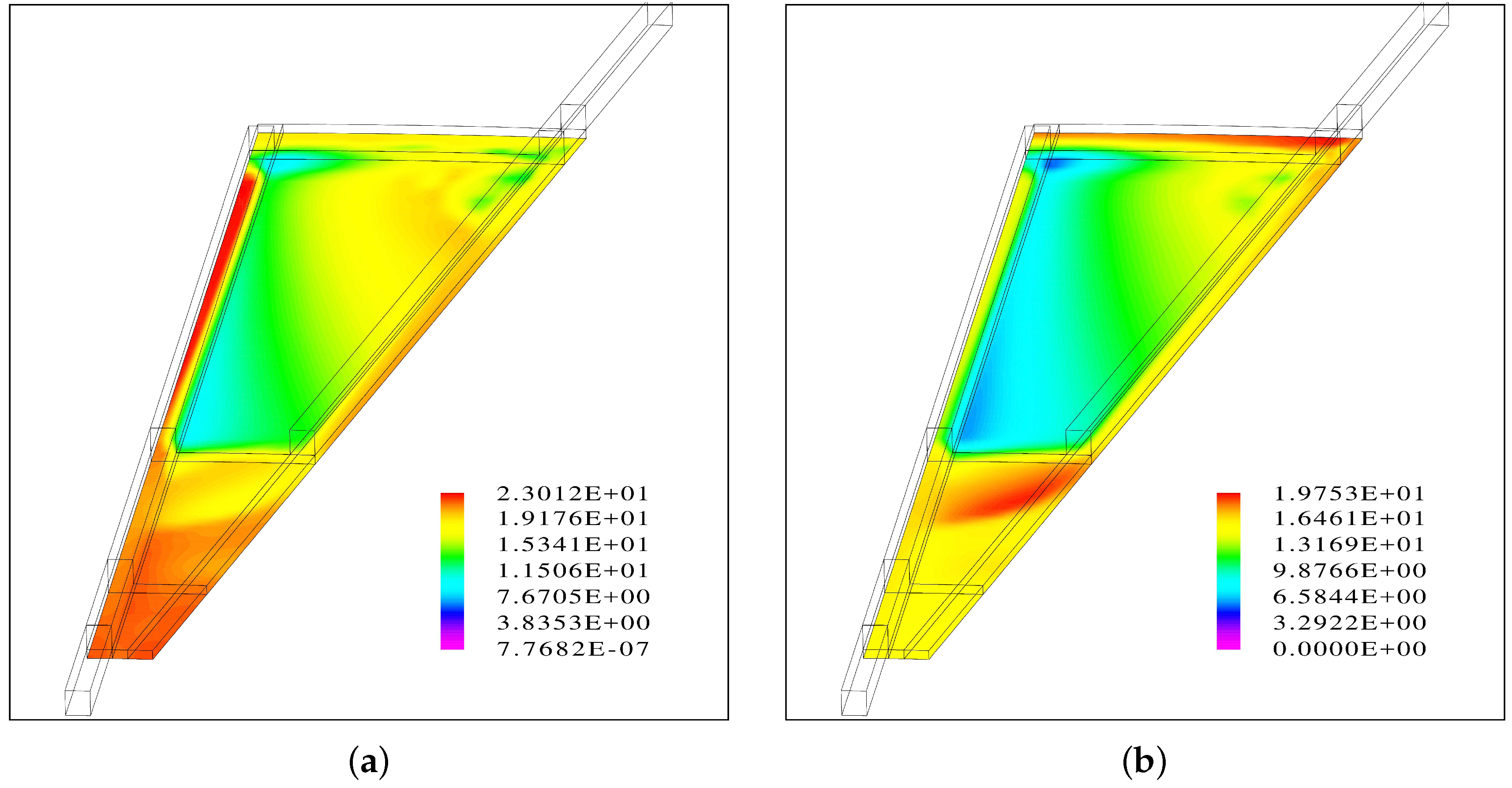
The distribution of the molar oxygen and water vapor concentration is shown in Figure 7. Not surprisingly, there are local maxima in the dry regions of the cell, while minima occur in the wet region between the two channels.
It is expected that the oxygen concentration is reduced when the operating pressure at the anode side is decreased [13], and that the ratio between the water vapor concentration and the oxygen molar concentration is accordingly increased. Detailed results of the water vapor to oxygen ratio will be presented in the parametric study section. However, it is not yet know, whether or how this concentration ratio affects the electrochemistry, and therefore these results are only of qualitative nature.
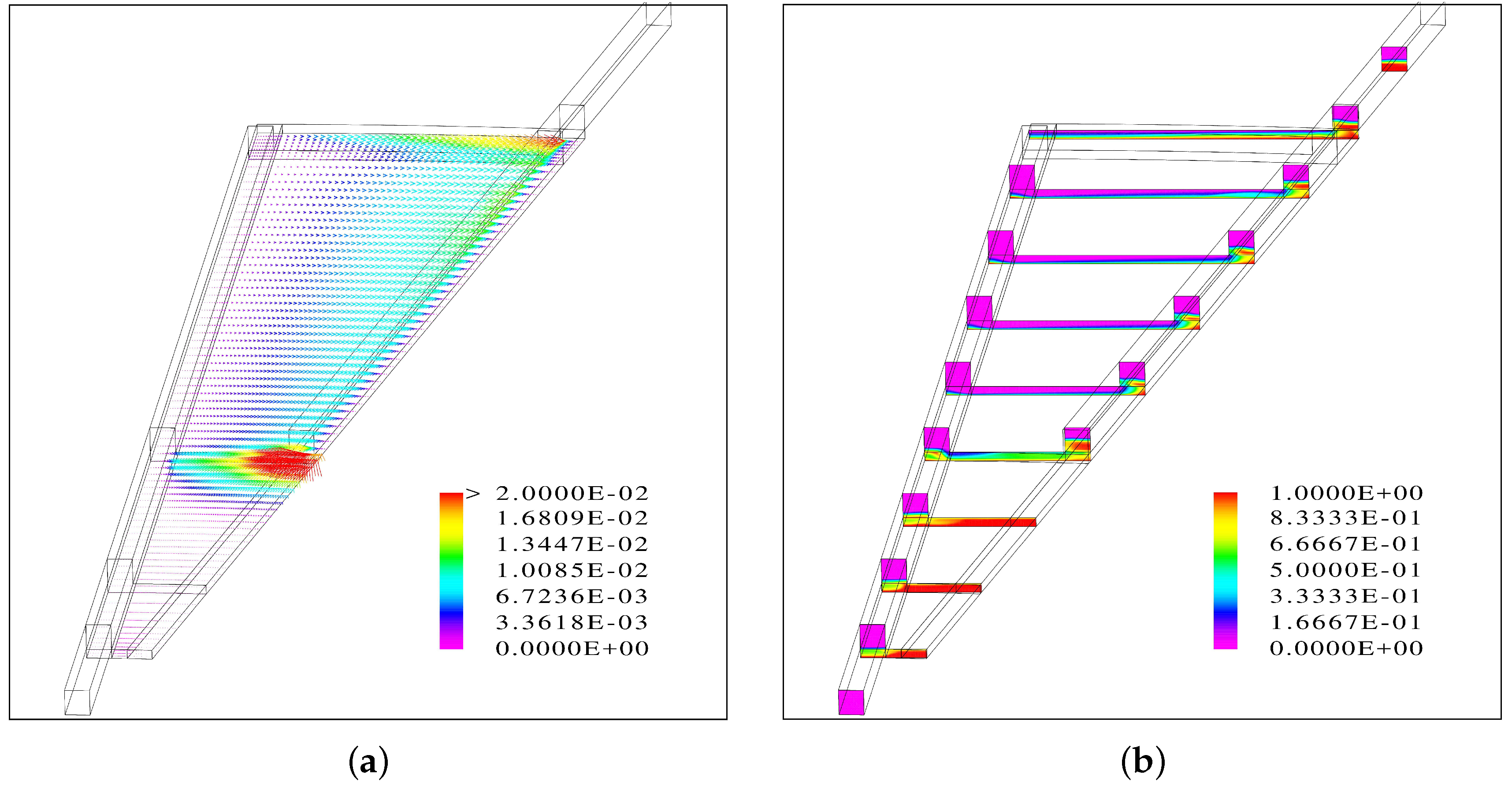
Figure 8 a) shows the gas phase velocity vectors and the speed used for coloring and the gas phase volume fraction. While the vectors are difficult to read, the local speed shows the maximum just before the outlet channel starts.
The distribution of the gas volume fraction, shown in Figure 8 b), is very interesting. The inlet channel is predicted to be almost exclusively in the liquid phase. This was intended in our design, but it as found that when the plate is turned around such that the flow channels are facing down (which is in fact the current orientation in our hardware), both the inlet channel and the outlet channel are in the multiphase region with segregated flow (not shown). With the current orientation where the channels are facing up and the water is pushed into the porous medium from below, the inlet channel is almost entirely filled with water, while there is segregated flow in the outlet channel, as expected. This is caused by the implementation of the drag forces here, equations 24 - 30, and it is encouraging to see that it leads to the desired results. The water stays in the bottom of the channel, but, as described, the flow is wavy and slightly pulsating. There is some gas phase predicted in the inlet channel before the outlet channel starts, in the region where the gas bubble was predicted. The coexistence of segregated channel flow and multiphase flow in porous together with heat transfer and phase change exemplified the numerical challenge of these cases, and they were difficult to converge.
However, seeing the complexity of the model, it is quite robust, and once a first converged solution was obtained, it was easy to conduct a parametric study. A result such as the pressure distribution agrees with expectation and gives confidence, and interesting findings such as the appearance of the gas bubble before the outlet channel begins have to be verified, but they suggest that there is room for improvement of the bipolar plate design.
3.2. Parametric Study Results
In the base case, the anode side was operated at ambient pressure, prescribed at the outlet. It was previously suggested that a reduction in anode side pressure with help of a vacuum pump is expected to favorably adjust the ratio between the water vapor concentration and the oxygen concentration [13]. Therefore, calculations were run with a different outlet pressure of 0.8 bar, 0.6 bar and 0.5 bar, respectively. At the operating temperature of 80 °C, the saturation pressure of water vapor is roughly 48 kPa (0.48 bar) and, if thermodynamic equilibrium prevails, the water vapor will be at this saturation pressure, corresponding to a relative humidity of 100%.
Generally, the distributions as shown and discussed for the base case remained very similar. An observation was that for a decreased operating pressure there is generally a larger gas fraction in the entire compartment. This is not unexpected because a lower pressure gas can accommodate a higher amount of water vapor, and therefore the evaporation terms have increased. This higher gas fraction leads to an increase in the gas phase mass flow rate, and thus to an increased pressure drop. While in the base case, the observed pressure drop was around 1418 Pa, this value increased to over 3303 Pa for a back pressure of 0.5 bar, i.e. it more than doubled, which is caused by the higher gas phase velocity.
The key outcome of the parametric study is the calculated ratio between the oxygen and the water vapor concentration in the gas phase because this is likely to have an effect on the electrolyzer performance. According to the Butler-Volmer equation and general reaction kinetics, a concentration ratio between reactant and product leads to more favorable reaction kinetics. Table 2 lists the average water vapor and oxygen concentrations at the PTL/CL interface as well as their ratio which increased by a factor of 5.6 between the lowest and the highest outlet pressure.
Finally, it is important to analyze the energy balance. In the electrolyzer, the only heat source is the waste heat produced. As mentioned above, it was assumed that the operating voltage is 1.85 V which leads to a heat source of 0.94 W for the investigated cell area of 1.57 cm2. In contrast to this heating term, there is the evaporative cooling. The amount of evaporation was calculated as part of the simulations, and a good first approximation is to assume that the oxygen gas leaving the cells is fully saturated, i.e. the relative humidity is equal to one:
According to Dalton’s law, we have:
out of which follows:
This can be reformulated into the desired expression for the molar flow rate of water vapor at the outlet:
where I is again the total current (here 1.57 A) and F is Faraday’s constant, yielding a molar oxygen flow of mole/s at the outlet. To approximate the evaporative cooling, this molar flow rate has to be multiplied with the molar heat of phase change at 80 °C, r=41.58 kJ/mole. Using a saturation pressure of water of 47.415 kPa at that temperature, the amount of evaporative cooling can be calculated as shown in Table 3, where the grey shaded cells correspond to these thermodynamic equilibrium calculations. Note that these values correspond to an outlet temperature of 80 °C, and are therefore only a rough approximation. The calculated cooling rates in Table 3 have to be compared with the heating term of 0.94 W due to the waste heat production. However, it has to be borne in mind that these values were calculated assuming thermodynamic equilibrium at the outlet at a temperature of 80 °C. If the temperature increases, the amount of evaporation will be higher, as is seen from the CFD results. Overall, the amount of phase change cooling at a high electrolyzer operation temperature is in the same order as the waste heat produced, and it can even exceed it so that the cell is cooled down. The last two columns in Table 3 summarize the CFD results. Because of temperature variations along with mass transport limitation, these values deviate from the values calculated from thermodynamic equilibrium.
It is also noted from Equation 51 that the amount of evaporation water shows a very high sensitivity to the operating temperature: the saturation pressure depends exponentially on the temperature according to Antoine’s equation, and an increase in temperature leads to both an increase in the numerator of Equation 51 and a decrease in the denominator, and as the outlet pressure approaches the saturation pressure, this fraction becomes very large so that the amount of water vapor leaving the cell becomes much larger than the amount of oxygen which only depends on the current density.
It can be concluded that reducing the outlet pressure drastically enhances the evaporative cooling, and in the current case, at a back pressure of 60 kPa the calculated heat of evaporation almost exactly balances the waste heat while at the lowest pressure investigated, the cell is in fact cooled down which makes this mode of operation unsustainable because the waste heat from the anode outlet is meant to preheat the incoming water in the integrated heat exchanger, such a low temperature increase is insufficient to allow sustainable operation. This means that the operating conditions have to be very carefully chosen in order to obtain sustainable electrolyzer operation, and future work is directed into identifying suitable operating conditions that end up in a temperature increase of a few °C while avoiding hot spots. Finally, it can be seen from Equation 51 that the amount of water that can evaporate is highly temperature dependent, and a small decrease in operating temperature will significantly bring down the amount of water that evaporates.
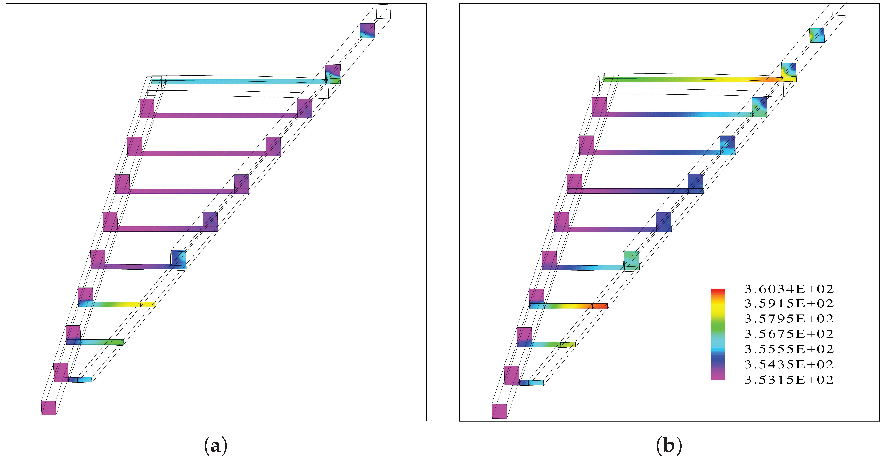
Figure 9 shows the calculated temperature distribution where the temperature distribution for 600 mbar and the base case with 1 atm back pressure are directly compared. Reducing the pressure leads to an overall cooler cell, but the minimum temperature remains at the nominal operating temperature, exemplifying the efficiency of evaporative cooling. Compared to the base case, the isothermal region has greatly expanded. The hot spot at the inlet section is predicted for both cases, but it is less severe for the lower back pressure. This also holds true for the hot region at the outer edge of the plate where the peak temperature is around 5 °C lower for the reduced back pressure. For the hot region near the inlet, it can be expected that when the beginning of the outlet channel is located closer to the center, i.e. the outlet channel is longer, the hot spot will be still less severe, and the section of the cell that experiences an almost uniform temperature will be expanded. The hot spot near the outlet appears to be caused by the higher outlet temperature, and it can be reduced by adjusting the back pressure.
4. Conclusions
In this work, a multiphase model for the anode side of a proton exchange membrane electrolyzer has been developed. The model is based on the Eulerian approach and thus solves a complete set of transport equations for each phase, in this case gas and liquid. The liquid phase consists of pure water while the gas phase contains oxygen and water vapor. Importantly, the model is non-isothermal and thus allows for the prediction of hot spots.
A base case was defined at a cell voltage of 1.85 V, a current density of 1 A/cm2 and a stoichiometry of . A quick analysis has shown that the expected flow in the horizontal channels should be segregated with a sharp interface between the liquid and gas phase. The following findings were made in detail:
- The results suggest that when the flow channels are facing up, the inlet channel is almost entirely filled with water while there is segregated flow in the outlet channel.
- Inside the porous medium, the gas phase accumulates at the top and a fraction of the liquid phase at the bottom, leading to a uniform distribution of the water vapor at the PTL/CL interface.
- A gas bubble is predicted near the center of the round plate before the outlet channel of the interdigitated flow field begins. This area coincides with a region of a hot spot with a temperature increase of 7 °C.
- A second hot spot with a similar temperature increase is predicted close to the outer edge near the outlet.
- From a modelling perspective, both buoyancy effects and phase change with the associated heating or cooling have to be accounted for.
- In agreement with both the Baker diagram as well as the Taitel and Dukler charts, the flow in the outlet channel was pulsating even when a "converged solution" was obtained. While slug flow can not be captured with a steady state model, it was also observed that the key results presented here were widely unaffected by the flow pattern in the outlet channel.
From the parametric study where the operating pressure was stepwise reduced, the following conclusions can be made:
- As intended, the concentration ratio between the water vapor and the oxygen can be adjusted in favor of the water vapor which is expected to yield a better performance. However, owing to thermal effects, the improvement is weaker than initially calculated. The concentration ratio between operating at ambient pressure and the lowest pressure investigated here of 50 kPa increased by a factor of 5.6.
- While the case with ambient back pressure predicted a temperature increase of around 4 °C from inlet to outlet, a decrease in back pressure resulted in a cooling effect due to increased evaporation. It can be concluded that reducing the outlet pressure is a viable method to keep the stack temperated when operating at even higher current densities.
- Thermal effects are important to account for. If the back pressure is adjusted to a too low value, the amount of evaporation can exceed the waste heat produced, and the electrolyzer outlet temperature is below the inlet temperature, which makes this particular operation mode unsustainable.
In the future, attention will be paid to identify suitable and sustainable operating conditions, and to better understand the impact of the plate orientation and channel geometry.
Author Contributions
Conceptualization, T.B.; methodology, T.B. and T.C.; software, T.B.; formal analysis, T.B. and T.C.; investigation, T.B. and T.C.; resources, T.B. and T.C.; data curation, T.B.; writing—original draft preparation, T.B.; writing—review and editing, T.B., and T.C.; visualization, T.B. and T.C. All authors have read and agreed to the published version of the manuscript.
Funding
The work received no funding.
Data Availability Statement
The original contributions presented in the study are included in the article, further inquiries can be directed to the corresponding author.
Conflicts of Interest
The authors declare no conflicts of interest.
References
- Schmidt, O.; Gambhir, A.; Staffell, I.; Hawkes, A.; Nelson, J.; Few, S. Future cost and performance of water electrolysis: An expert elicitation study. International Journal of Hydrogen Energy 2017, 42, 30470–30492. [Google Scholar] [CrossRef]
- Feng, Q.; Yuan, X.; Liu, G.; Wei, B.; Zhang, Z.; Li, H.; Wang, H. A review of proton exchange membrane water electrolysis on degradation mechanisms and mitigation strategies. Journal of Power Sources 2017, 366, 33–55. [Google Scholar] [CrossRef]
- Grigoriev, S.; Porembskiy, V.; Korobtsev, S.; Fateev, V.; Auprêtre, F.; Millet, P. High-pressure PEM water electrolysis and corresponding safety issues. International Journal of Hydrogen Energy 2011, 36, 2721–2728. [Google Scholar] [CrossRef]
- Nie, J.; Chen, Y. Numerical modeling of three-dimensional two-phase gas–liquid flow in the flow field plate of a PEM electrolysis cell. International Journal of Hydrogen Energy 2010, 35, 3183–3197. [Google Scholar] [CrossRef]
- Olesen, A.C.; Rømer, C.; Kær, S.K. A numerical study of the gas-liquid, two-phase flow maldistribution in the anode of a high pressure PEM water electrolysis cell. International Journal of Hydrogen Energy 2016, 41, 52–68. [Google Scholar] [CrossRef]
- Lafmejani, S.S.; Olesen, A.C.; Kær, S.K. VOF modelling of gas–liquid flow in PEM water electrolysis cell micro-channels. International Journal of Hydrogen Energy 2017, 42, 16333–16344. [Google Scholar] [CrossRef]
- Zinser, A.; Papakonstantinou, G.; Sundmacher, K. Analysis of mass transport processes in the anodic porous transport layer in PEM water electrolysers. International Journal of Hydrogen Energy 2019, 44, 28077–28087. [Google Scholar] [CrossRef]
- Upadhyay, M.; Lee, S.; Jung, S.; Choi, Y.; Moon, S.; Lim, H. Systematic assessment of the anode flow field hydrodynamics in a new circular PEM water electrolyser. International Journal of Hydrogen Energy 2020, 45, 20765–20775. [Google Scholar] [CrossRef]
- Millet, P.; Ngameni, R.; Grigoriev, S.; Fateev, V. Scientific and engineering issues related to PEM technology: Water electrolysers, fuel cells and unitized regenerative systems. International Journal of Hydrogen Energy 2011, 36, 4156–4163. [Google Scholar] [CrossRef]
- Upadhyay, M.; Kim, A.; Paramanantham, S.S.; Kim, H.; Lim, D.; Lee, S.; Moon, S.; Lim, H. Three-dimensional CFD simulation of proton exchange membrane water electrolyser: Performance assessment under different condition. Applied Energy 2022, 306, 118016. [Google Scholar] [CrossRef]
- Falcão, D.; Pinto, A. A review on PEM electrolyzer modelling: Guidelines for beginners. Journal of Cleaner Production 2020, 261, 121184. [Google Scholar] [CrossRef]
- Su, X.; Zhang, Q.; Xu, L.; Hu, B.; Wu, X.; Qin, T. A novel combined flow field design and performance analysis of proton exchange membrane electrolysis cell. International Journal of Hydrogen Energy 2024, 61, 444–459. [Google Scholar] [CrossRef]
- Berning, T. Design of a Proton Exchange Membrane Electrolyzer. Hydrogen 2025, 6. [Google Scholar] [CrossRef]
- Marshall, A.; Børresen, B.; Hagen, G.; Tsypkin, M.; Tunold, R. Hydrogen production by advanced proton exchange membrane (PEM) water electrolysers—Reduced energy consumption by improved electrocatalysis. Energy 2007, 32, 431–436. [Google Scholar] [CrossRef]
- Millet, P.; Ngameni, R.; Grigoriev, S.; Mbemba, N.; Brisset, F.; Ranjbari, A.; Etiévant, C. PEM water electrolyzers: From electrocatalysis to stack development. International Journal of Hydrogen Energy 2010, 35, 5043–5052. [Google Scholar] [CrossRef]
- Berning, T.; Djilali, N. A 3D, Multiphase, Multicomponent Model of the Cathode and Anode of a PEM Fuel Cell. Journal of The Electrochemical Society 2003, 150, A1589. [Google Scholar] [CrossRef]
- Gurau, V.; Zawodzinski, Thomas A. , J.; Mann, J. Adin, J. Two-Phase Transport in PEM Fuel Cell Cathodes. Journal of Fuel Cell Science and Technology 2008, 5, 021009. [Google Scholar] [CrossRef]
- Baker, O. Design of Pipelines for the Simultaneous Flow of Oil and Gas. 1953.
- Scott, D.S. Properties of Cocurrent Gas-Liquid Flow; Academic Press, 1964; Vol. 4, Advances in Chemical Engineering, pp. 199–277. [CrossRef]
- Taitel, Y.; Dukler, A.E. A model for predicting flow regime transitions in horizontal and near horizontal gas-liquid flow. AIChE Journal 1976, 22, 47–55. [Google Scholar] [CrossRef]
- Bird, R.; Stewart, W.; Lightfoot, E. Transport Phenomena; Number v. 1 in Transport Phenomena, Wiley, 2006.
- Nam, J.H.; Kaviany, M. Effective diffusivity and water-saturation distribution in single-and two-layer PEMFC diffusion medium. International Journal of Heat and Mass Transfer 2003, 46, 4595–4611. [Google Scholar] [CrossRef]
- Olesen, A.C.; Kær, S.K.; Berning, T. A Multi-Fluid Model for Water and Methanol Transport in a Direct Methanol Fuel Cell. Energies 2022, 15. [Google Scholar] [CrossRef]
- Marrero, T.R.; Mason, E.A. Gaseous Diffusion Coefficients. Journal of Physical and Chemical Reference Data 1972, 1, 3–118. [Google Scholar] [CrossRef]
- Grigoriev, S.; Millet, P.; Volobuev, S.; Fateev, V. Optimization of porous current collectors for PEM water electrolysers. International Journal of Hydrogen Energy 2009, 34, 4968–4973. [Google Scholar] [CrossRef]
- Barbir, F. PEM fuel cells: theory and practice; Academic press, 2012.
Figure 1.
PEM electrolyzer schematic.
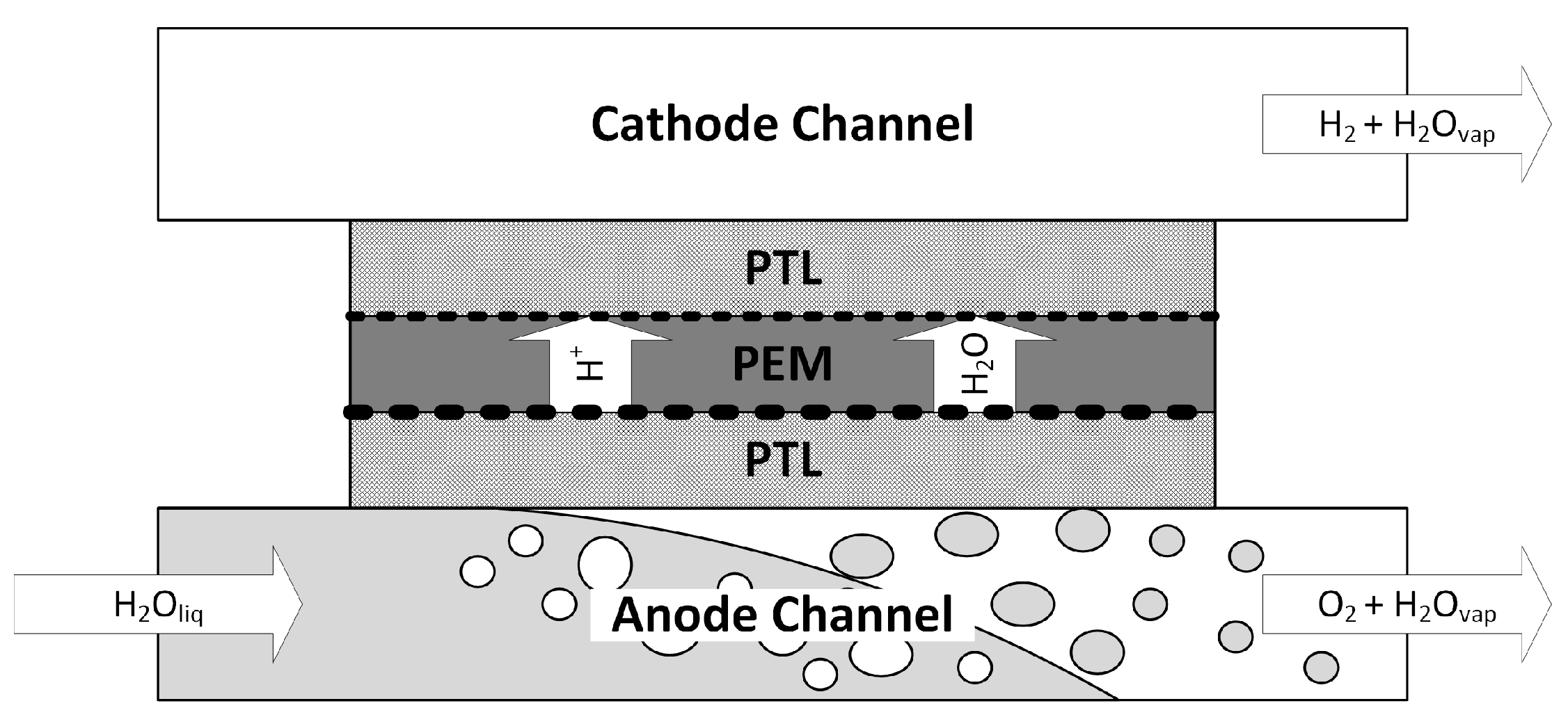
Figure 2.
Anode flow field of the investigated electrolyzer design. The water enters from the center.
Figure 2.
Anode flow field of the investigated electrolyzer design. The water enters from the center.
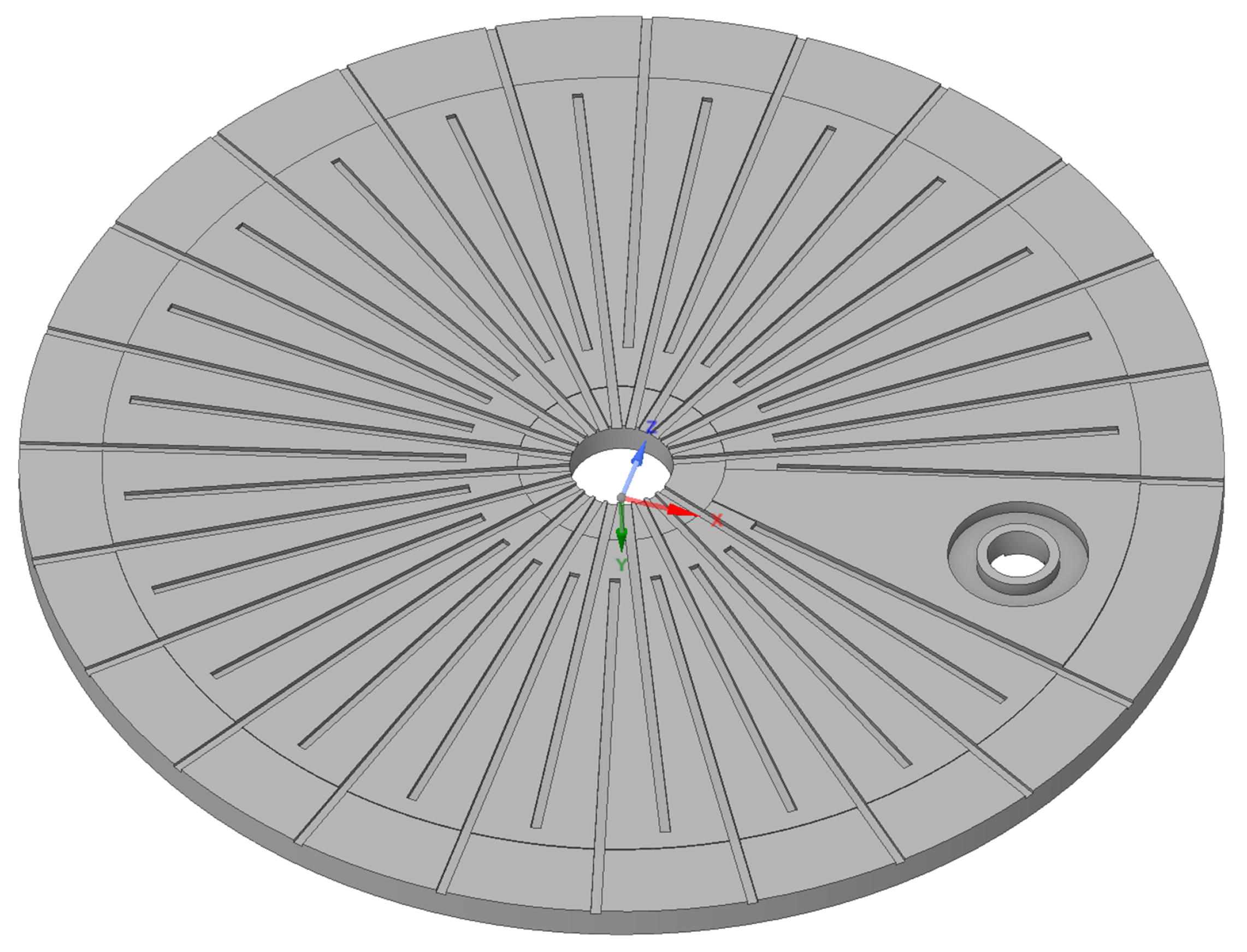
Figure 3.
(a) Computational domain and lock structure and (b) computational grid employed in this study.
Figure 3.
(a) Computational domain and lock structure and (b) computational grid employed in this study.
| (a) | (b) |
Figure 4.
Schematic of a modified Baker diagram for flow in horizontal pipes with flow patterns.
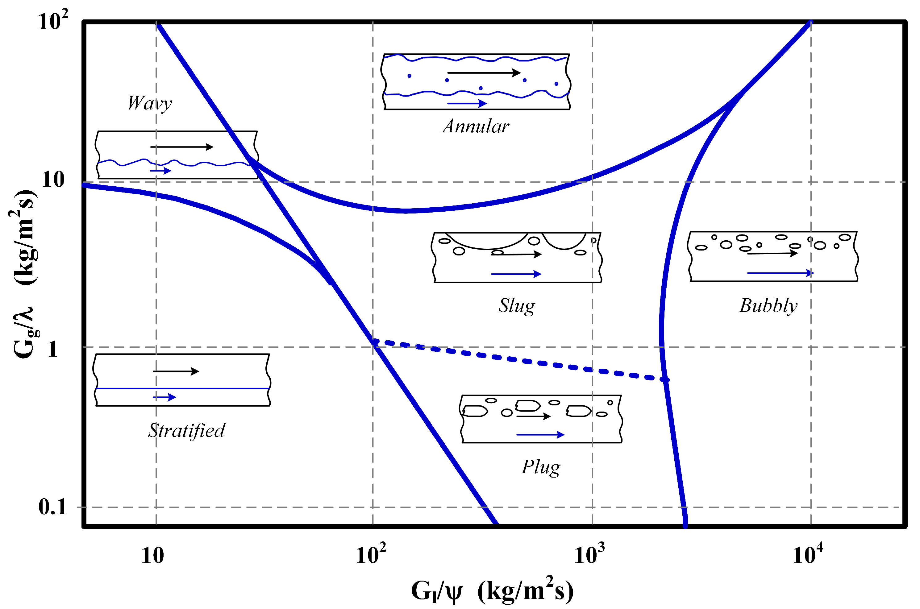
Figure 5.
(a) Relative pressure [Pa] and (b) absolute temperature [K] distribution at the GDL/CL interface.
Figure 5.
(a) Relative pressure [Pa] and (b) absolute temperature [K] distribution at the GDL/CL interface.
| (a) | (b) |
Figure 6.
(a) Gas volume fraction [-] and (b) evaporation rate [kg/m3s] at the GDL/CL interface.
| (a) | (b) |
Figure 7.
(a) Molar oxygen concentration [mol/m3] and (b) molar water vapor concentration [mol/m3] at the GDL/CL interface.
Figure 7.
(a) Molar oxygen concentration [mol/m3] and (b) molar water vapor concentration [mol/m3] at the GDL/CL interface.
| (a) | (b) |
Figure 8.
(a) Velocity vectors colored by the speed and (b) gas phase volume fraction in different planes down the y-axis.
Figure 8.
(a) Velocity vectors colored by the speed and (b) gas phase volume fraction in different planes down the y-axis.
| (a) | (b) |
Figure 9.
(a) Temperature distribution in [K] for (a) 600 mbar total pressure and (b) 1,013 mbar back pressure. The inlet temperature is 353.15 K and the legend applies to both plots.
Figure 9.
(a) Temperature distribution in [K] for (a) 600 mbar total pressure and (b) 1,013 mbar back pressure. The inlet temperature is 353.15 K and the legend applies to both plots.
| (a) | (b) |
Table 2.
Water vapor and oxygen concentrations at the GDL/CL interface.
| Back Pressure | : | ||
|---|---|---|---|
| [kPa] | [mol/m3] | [mol/m3] | [-] |
| 101.3 | 13.07 | 17.29 | 0.76 |
| 80.0 | 14.36 | 11.45 | 1.25 |
| 60.0 | 15.22 | 5.07 | 3.00 |
| 50.0 | 14.71 | 3.44 | 4.27 |
Table 3.
Molar flow rates and cooling power for thermodynamic equilibrium (gray cells) and CFD results (last two columns).
Table 3.
Molar flow rates and cooling power for thermodynamic equilibrium (gray cells) and CFD results (last two columns).
| Back Pressure | |||||
|---|---|---|---|---|---|
| [kPa] | [mole/s] | [mole/s] | [W] | [mole/s] | [W] |
| 101.3 | -0.15 | -0.49 | |||
| 80 | -0.25 | -0.63 | |||
| 60 | -0.64 | -0.99 | |||
| 50 | -3.10 | -1.18 |
Disclaimer/Publisher’s Note: The statements, opinions and data contained in all publications are solely those of the individual author(s) and contributor(s) and not of MDPI and/or the editor(s). MDPI and/or the editor(s) disclaim responsibility for any injury to people or property resulting from any ideas, methods, instructions or products referred to in the content. |
© 2025 by the authors. Licensee MDPI, Basel, Switzerland. This article is an open access article distributed under the terms and conditions of the Creative Commons Attribution (CC BY) license (http://creativecommons.org/licenses/by/4.0/).
Copyright: This open access article is published under a Creative Commons CC BY 4.0 license, which permit the free download, distribution, and reuse, provided that the author and preprint are cited in any reuse.


