1. Introduction
The topic of stability has generated worldwide attention, particularly with the emergence of formal regulatory standards such as those introduced by the International Conference on Harmonization (ICH). The ICH quality (Q) guideline has evolved significant development across various documents (Q1A-A1F) to provide more comprehensive descriptions of stability testing principles [
1].
Q1A(R) was published in 1994 and outlines the requirements for stability data packages concerning new drug substances or drug products. It specifies recommended storage conditions, test parameters, and acceptance criteria essential for assessing the stability of pharmaceutical products. Additionally, the Q1(E) guideline, introduced in 2003, further contributes to this framework. It guides utilizing stability data generated following the principles outlined in the ICH guideline “Q1A(R) Stability Testing of New Drug Substances and Products”. Moreover, it describes the methodology for extrapolating data when proposing a retest period for a drug substance or a shelf life for a drug product that exceeds the timeframe covered by “available data from the stability study conducted under the long-term storage condition” [
2]. Hence, stability studies are imperative after the examination of both Q1A(R) and Q1(E) guidelines to determine suitable storage conditions and expiry dates [
2,
3]. These standard stability assessments are essential not only for furnishing data to validate drug registration with regulatory bodies, but also for establishing and sustaining the quality of products [
4]. Specifically, stability studies are employed to forecast long-term stability and to ascertain degradation rates and kinetics by analyzing data obtained under various storage conditions [
5].
The generation of stability data constitutes a crucial component of a drug product’s life cycle [
6]. Assessing stability has emerged as an imperative to forecast the prolongation of shelf-life for medicines [
7]. Various statistical methodologies can be employed to recognize patterns and predict the behavior of drug products [
8]. However, the practical implementation of these statistical approaches is not addressed in detail within the ICH guideline Q1E [
2]. Moreover, recent guidelines concerning stability data provide only general theoretical prerequisites and lack practical insights for evaluating this aspect.
Recently, Capen et al. assessed a simple linear regression model (SLR), suggesting its adequacy in describing the observed data derived from a stability study [
9].
Additionally, the use of SLR techniques and the empirical cumulative distribution function has shown promise in predicting the probability of drug product failure over its shelf-life [
6]. Several studies have already deliberated on statistical methods and approaches to evaluate stability concerns of drug products throughout their shelf-life. For instance, Binbing et al. devised three distinct statistical methods to identify the out-of-trend (OOT) result in stability studies [
7]. Lyon et al. highlighted the use of regression analysis to predict real-time stability data [
10]. Furthermore, Mihalovits et al. documented an adaption of the SLR method for detecting OOT points within pharmaceutical stability studies [
11]. The application of the SLR technique has also been documented and reported in various drug formulations, including liquid drug formulations [
12] and tablet formulations [
13]. Hence, it is reasonable to conclude that the “SLR” technique represents a suitable statistical approach for stability studies.
The primary focus of this paper is to elucidate the difference between change and variability, as mentioned in guideline Q1E. Additionally, the study aims to assess the efficacy of the Simple Linear Regression approach (SLR-CI), Confidence Interval on Slop and Intercept (S&I-CI) and Predictive Interval (PI) techniques in determining the supported shelf-life period under different conditions and to highlight its significance. For this purpose, the paper initially introduces the prediction intervals technique. The technique is subsequently discussed in detail to elucidate the variability in stability. Finally, the retest period or shelf-life estimation is used for determining a stability uncertainty.
2. Materials and Methods
2.1. Statistical Background
In Appendix 1 of guideline Q1E, the focus lies on assessing the change or variability of stability. This involves whether there are little changes or little variability during the accelerated, intermediate, and real conditions [
2]. Establishing a drug product’s shelf-life period necessitates obtaining evidence of change and variability before defining this period.
According to the Oxford Dictionary, variability refers to the likelihood of something varying, while change involves making somebody/something different. In statistics, variability can be quantified using various tools, and the choice of tool often depends on the level of measurement of the variable. In stability studies, different statistical measures such as range, interquartile range, standard deviation, and variance are commonly used to assess the variability. Each of these tools offers unique insights into the degree of variability present within the data set [
14,
15].
As per the Cambridge Dictionary of Statistics, the range represents the difference between the highest and lowest observations within a dataset. While it’s commonly used as a straightforward method to estimate dispersion, it’s not typically recommended for this purpose due to its sensitivity to outliers and the fact that its value increases with larger sample sizes [
16].
Interquartile range is a statistical measure of spread, defined as the difference between the first and third quartiles of a sample. It provides insight into the dispersion of data while being less affected by outliers compared to the range [
17].
The standard deviation is widely recognized as the most used measure for assessing the spread of a set of observations. It is calculated as the square root of the variance, and it is often considered suitable for evaluating stability data [
18].
On the other hand, change denotes a variation in the value of a statistic before and after a specific event or over a while. It can also signify the degree of difference between two or more statistics [
19]. Various methods for assessing change and variability exist contingent upon the context and the nature of the data being analyzed, namely: basic statistics, confidence interval, and predictive interval.
2.2. Basic Statistics
To estimate absolute change, the method involves finding the difference between the initial value and final values of a statistic.
The relative change is expressed according to the equation bellow:
The percentage change is expressed by the following equation:
2.3. Stability Evaluation
The usual test to detect a statistically significant gradient is a t-test for a slope very different from zero, this test is performed by calculating the t-statistic using the following formula:
With b1 is the slop and s(b1) is the slop standard deviation.
Decision: The comparison of this statistic to a critical bilateral t-student value (degrees of freedom = n-2) with a confidence level of 95% is conducted. If the calculated statistic, , is greater than the critical value, we conclude that the slope is different from zero with a confidence level of 95%, and therefore, the stability is not assumed.
2.4. Statistical Interval
2.4.1. Confidence Interval
Confidence intervals are useful for assessing the variation around a point estimate [
20], they are estimated through the following equation:
Where CI is the confidence interval, X̄ is the sample mean, Z is the critical value of the t distribution, σ is the sample standard deviation and √n is the square root of the sample size.
2.4.2. Prediction Interval
A prediction interval is defined as an interval in which, with a given probability, the future result(s) should fall, given the already observed results. A prediction interval for a single future observation is an interval that will, with a specified degree of confidence, contain the next randomly selected observation from a population. Prediction intervals containing all of the m future observations are often of interest to manufacturers of large equipment who produce only a small number of units of a particular type of product [
21].
Where
is the predicted value,
is the quantile of the student t distribution with n-2 degrees of freedom (
) and
is the standard error of the prediction.
Where Sy is the residual standard deviation, is the mean of the measured value, is the true value (reference) and is the sample standard deviation.
Finally, the prediction interval can be expressed as:
2.5. Stability Uncertainty
The uncertainty associated with the content of the compound of interest is calculated using the following formula:
With:
: Slope standard deviation,
: Shelf-life period defined within stability evaluation within real conditions.
3. Results
In this section, we implement the methodology outlined in section method to analyze the outcome from Faya’s paper [
12]. For the accelerated study, data is sourced from
Table 1, encompassing assay results for four temperatures at various time points, all over a three-month timeframe.
Applying the statistical parameters outlined in section 2.1, the assessment of outcomes presented in
Table 1 offers some insights within accelerated stability study. It appears that the most significant changes or variations are observed at high temperatures (
Table 2). However, aligning with these outcomes and drawing crucial conclusions proves challenging. It’s evident that relying on the initial evaluation is insufficient for definitive conclusions. Therefore, exploring additional tools for relevant conclusions becomes necessary.
Likewise, with the confidence interval provided in
Table 3, pertinent conclusions remained ambiguous, unless considering the width of the interval, which becomes notably significant at higher temperatures.
Due to the ambiguity stemming from these findings, we opt to employ the stability evaluation discussed in section 2.5, focusing not only on demonstrating changes or variability, but also on assessing the overall stability of the data.
Based on the results obtained in
Table 4, the calculated statistics for temperatures 35 °C, 45 °C, and 65 °C fall below the critical value. Consequently, we conclude that the slope is equal to zero with a confidence level of 95%, and therefore, the stability is assumed. At a temperature of 55 °C, stability is not assumed because the statistical hypothesis of stability has been rejected. Eventually, it suggests that further progression to 65 °C may not be necessary.
The next step is to assess the stability of the drug in the long-term study (
Table 5). Then, we’ll need to extrapolate the data to determine the drug’s shelf life.
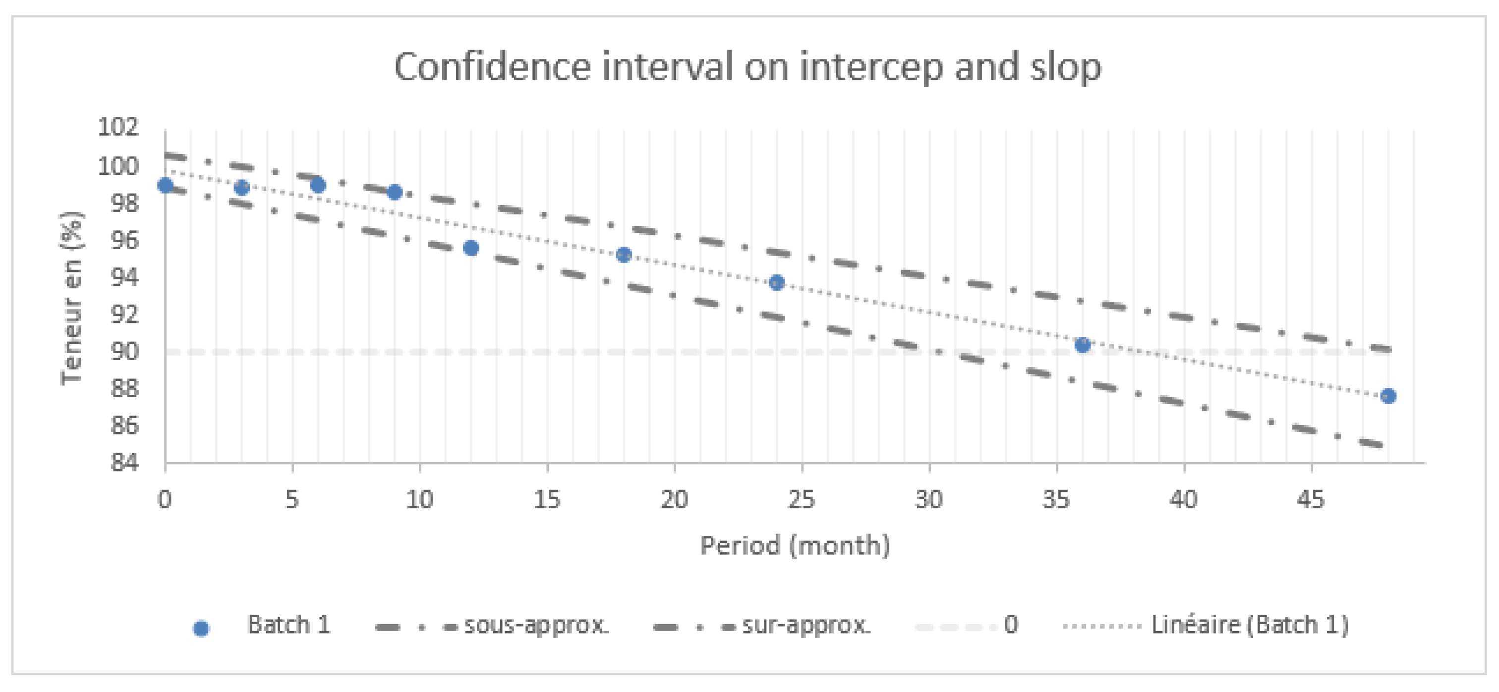
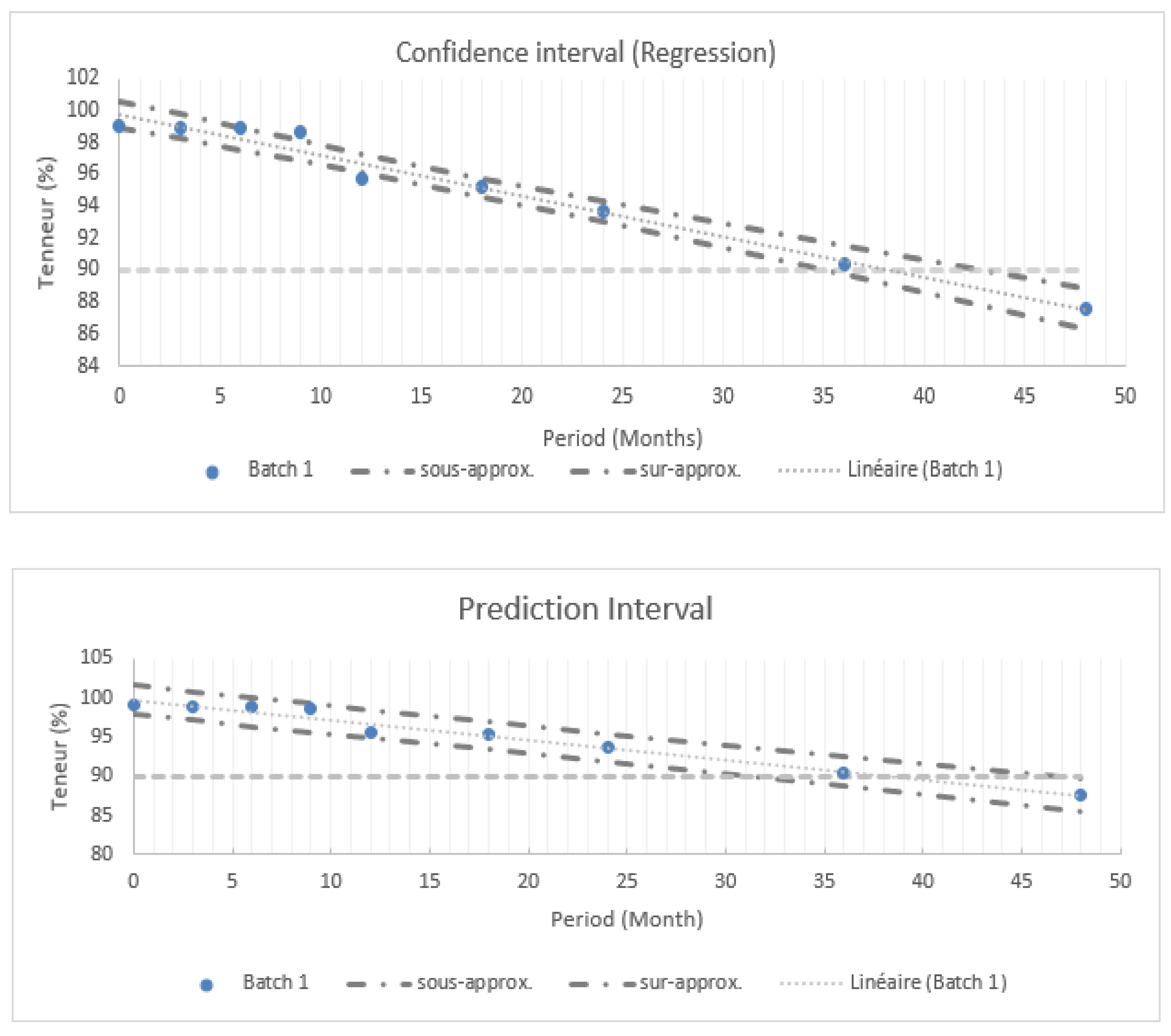
Based on the findings presented in
Figure 1, various statistical intervals are used to assess the drug shelf-life.
Figure 1 summarizes statistical intervals at 95% including confidence and prediction intervals for batch 1.
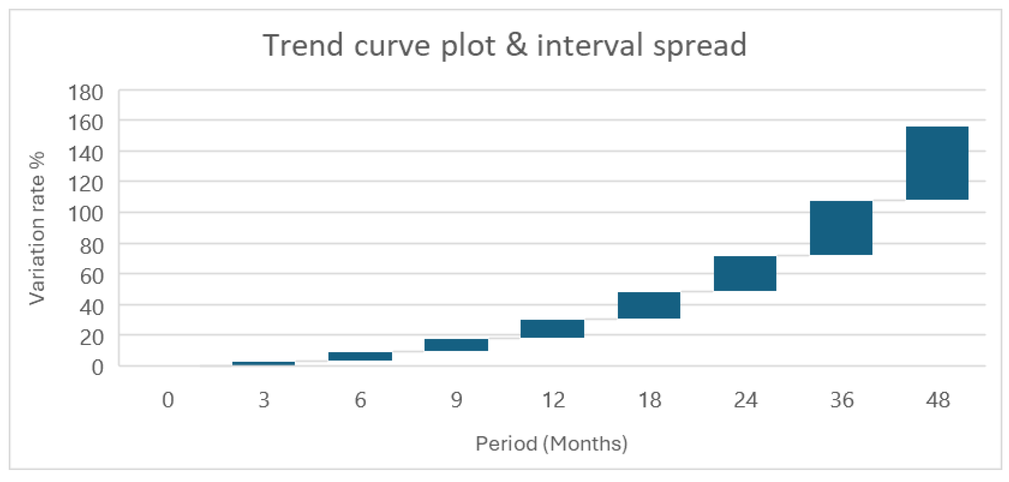
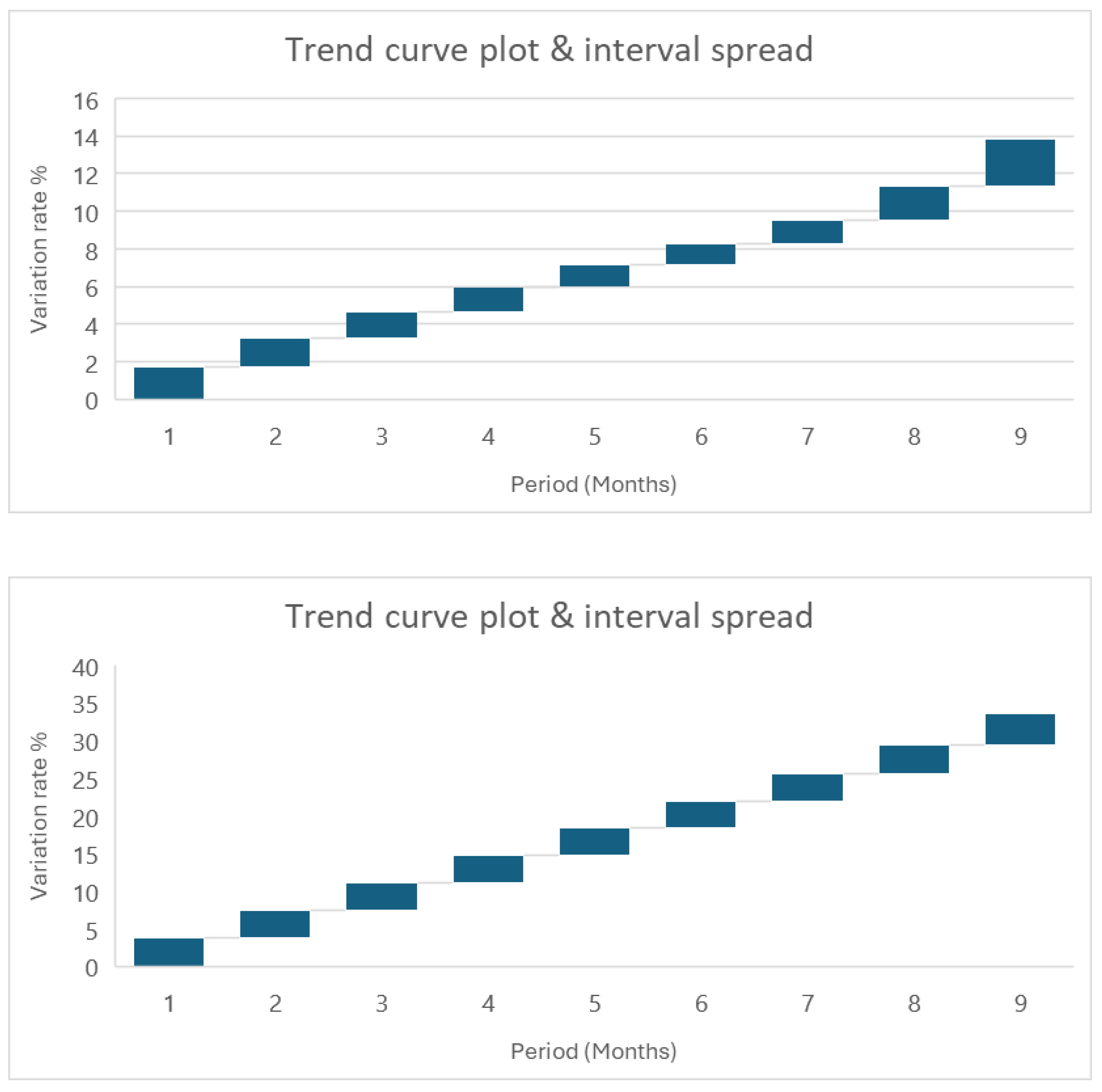
Figure 2 shows that different variations in interval spread are evident across statistical intervals application. The first plot displays a consistent exponential trend, with important variation evolving with time. Conversely, the second plot demonstrates an initial phase of variability, followed by a gradual decline over the half period of time; however, towards the end of the assessment period, variability resurges noticeably. More importantly, featuring with prediction intervals exhibits a steady interval spread throughout the assessed period.
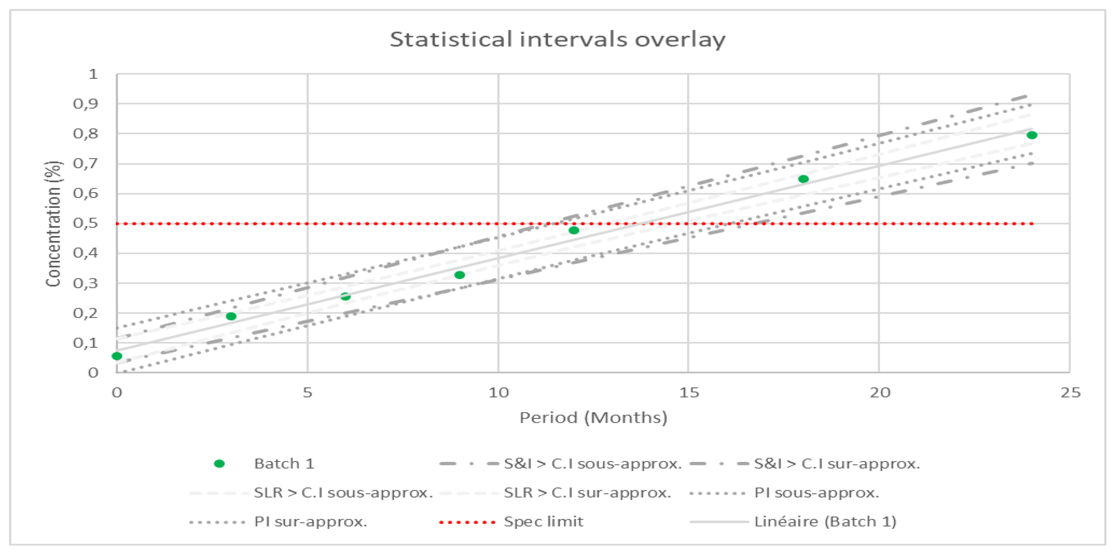
The same evaluations were conducted on the related substances, and the results obtained are presented as an overlay to illustrate the differences among all approaches.
The results are graphically summarized in
Figure 3, with the specification limit indicated by a red vertical line. Across all evaluations, the PI approach demonstrates a more balanced trend compared to the SLR and S&I approaches. Notably, the data from batch 1 overlaps with the confidence interval of SL, however, with the PI approach, no data points overlap the limit interval.
The results obtained further to uncertainty assessment in stability study for all approaches are presented in the
Table 6.
4. Discussion
The shelf-life assessment depends on how the data obtained after physical and chemical tests is managed. During the early drug development stage, where little information about the product or formulation is known, the test results from earlier time points are set as the norm for later time points [
22]. During the same stage, a shelf-life must be assigned, it includes the use of various factors to determine how long a product will be safe and effective for the patient under reasonable storage conditions. In the determination of the shelf-life, one generally measures a value that changes with time. Yet there are generally insufficient time points in a stability study to explicitly determine the functional form of the changes concerning time [
23].
In this paper, we demonstrate that the statistical intervals approach is highly effective for evaluating stability and determining the drugs shelf-life under different environmental storage conditions. However, conventional literature methods, which often rely on complex statistical techniques that may be challenging for a chemist to implement. Typical examples of statistical approaches that have been reported include the Bayesian approach [
24], combining the Arrhenius equation with the kinetic reaction equation [
25,
26], and advanced kinetic modeling [
23].
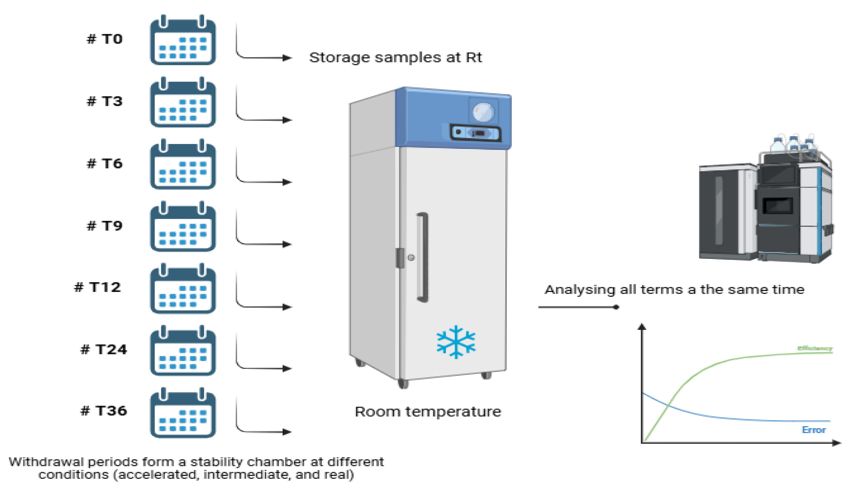
To implement our approach, we first conducted stability evaluations through accelerated studies to identify any significant changes or variability. Our findings demonstrate the potential to predict the shelf-life of medicine at earlier stages with minimal data. However, prior evaluations of the accelerated stability study (
Table 4) suggest that stability within 55 °C is not guaranteed, indicating the need for alternative actions before proceeding to analyze the next temperature point. Indeed, when producing a drug substance, synergies between pilot batch and production may be similar. The pilot batch could, therefore, help the manufacturer. In a true sense, a comprehensive literature study on an established molecule can save multiple generic manufacturers from conducting redundant basic studies, thereby avoiding wastage of resources [
27]. The estimation of medicine shelf-life from the pilot batch will be validated by the isochronous design and used as a proof during industrial production for stability evaluation. The isochronous stability evaluation approach is implemented as follows:
Figure 4.
Isochrone plan for stability evaluation.
Figure 4.
Isochrone plan for stability evaluation.
If the stability assessment has not been carried out at an earlier stage, it is carried out in parallel with the production of the batch of medicinal products.
Based on the long-term stability study results, we used three statistical intervals, namely, Confidence interval on Simple Linear Regression (SLR-CI), Confidence Interval on Slop and Intercept (S&I-CI) and Predictive Interval (PI). The drug shelf-life is exactly defined by the intersection between the specification limit and the extrapolation line. Our analysis revealed that among the three potency profiles evaluated, the SLR approach yielded the longest shelf-life period of 35 months. In contrast, the S&I approach provided a shelf-life period of 30 months, while the PI approach offered a period of 31 months. Furthermore, we integrated additional elements such as trend curve plots, interval spreads, and the intersection of the data (
Table 5) with the SLR interval to determine the most effective period. Considering all these tools, we concluded that the most optimal period could be provided by the PI interval, which demonstrates a balanced trend with minimal variability and a prolongation over 31 months, within a variation interval of ±1,2%
5. Conclusions
Scientific methodologies are crucial for elucidating the behavior of drugs and active ingredients under various environmental conditions. Assessing stability under accelerated conditions is essential, as it provides a foundational basis for extrapolating findings from samples to the broader population and offers insights into change and variability.
When designing a stability evaluation, it’s essential to incorporate the Predictive Interval approach. This method allows a more accurate estimation of variability by determining the range of values within which future observations are expected to occur, typically at the 95% confidence level.
Furthermore, conducting a stability study, using the isochronous approach for example, proposed in the discussion section, can save time and resources by eliminating the need for redundant basic studies in the future for the same substance of interest in the absence of raw material and production process variability. This approach enables tests to be carried out under repeatability conditions, thereby avoiding situations of equipment drift that may arise over the study period of 0 - 48 months. Fluctuating analysis conditions over time can introduce uncontrollable systematic errors, leading to sometimes contradictory results.
To address these issues, we propose including a new section in the drug leaflet that defines the shelf-life period and provides a graphical representation. This will ensure clarity and prevent misunderstandings regarding the stability and usability of the drug over time.
Author Contributions
Y.H. Benchekroun. conceived and designed the study. Collected the data and performed the experiments. M. Outaki. analyzed the data, drafted the manuscript, and provided critical revisions. All authors reviewed and approved the final manuscript.
Funding
This research received no external funding.
Data Availability Statement
All data supporting the findings of this study are available within the paper and its Supplementary Information. The data used in this study was sourced from the following paper: Faya P, Seaman Jr JW, Stamey JD. Using accelerated drug stability results to inform long-term studies in shelf-life determination. Statistics in Medicine. 2018; 37: 2599 2615.
https://doi.org/10.1002/sim.7663.
Conflicts of Interest
The authors declare no conflicts of interest.
References
- Jamrógiewicz, M. & Pieńkowska, K. (2019) TrAC Trends in Analytical Chemistry 111, 118–127. [CrossRef]
- Guideline, I.C.H.H.T. (2003) ICH Q1E. ICH 6, 1–19.
- Guideline, I.H.T. (2003) Q1A (R2), current step 4.
- Khan, H., Ali, M., Ahuja, A., & Ali, J. (2010) Curr Pharm Anal 6, 142–150. [CrossRef]
- Huynh-Ba, K. (2009) Handbook of stability testing in pharmaceutical development: regulations, methodologies, and best practices, Springer. [CrossRef]
- Suresh Kumar, B. V, Kulshrestha, P., & Shiromani, S. (2018) Methods for Stability Testing of Pharmaceuticals 233–260. [CrossRef]
- Yu, B., Zeng, L., Ren, P., & Yang, H. (2018) Stat Biopharm Res 10, 237–243.
- Schneid, S.C., Stärtzel, P.M., Lettner, P., & Gieseler, H. (2011) Pharm Dev Technol 16, 583–590. [CrossRef]
- Capen, R., Christopher, D., Forenzo, P., Huynh-Ba, K., LeBlond, D., Liu, O., O’Neill, J., Patterson, N., Quinlan, M., & Rajagopalan, R. (2018) AAPS PharmSciTech 19, 668–680. [CrossRef]
- Lyon, R.C., Taylor, J.S., Porter, D.A., Prasanna, H.R., & Hussain, A.S. (2006) J Pharm Sci 95, 1549–1560. [CrossRef]
- Mihalovits, M. & Kemény, S. (2020) J Pharm Biomed Anal 188, 113375. [CrossRef]
- Faya, P., Seaman Jr, J.W., & Stamey, J.D. (2018) Stat Med 37, 2599–2615. [CrossRef]
- Buda, V., Baul, B., Andor, M., Man, D.E., Ledeţi, A., Vlase, G., Vlase, T., Danciu, C., Matusz, P., & Peter, F. (2020) Pharmaceutics 12, 86. [CrossRef]
- David, H.A. (1998) Statistical Science 368–377.
- Dodge, Y. (2003) The Oxford dictionary of statistical terms, Oxford University Press, USA.
- Everitt, B.S. & Skrondal, A. (2010).
- Islam, M.A., Al-Shiha, A., Islam, M.A., & Al-Shiha, A. (2018) Foundations of Biostatistics 39–72. [CrossRef]
- Frost, J. (2022) Statistics by Jim. https://statisticsbyjim.com/basics/standard-deviation.
- Frost, J. (2021) Statistics by Jim.
- Wang, E.W., Ghogomu, N., Voelker, C.C.J., Rich, J.T., Paniello, R.C., Nussenbaum, B., Karni, R.J., & Neely, J.G. (2009) Otolaryngology—Head and Neck Surgery 140, 794–799. [CrossRef]
- Meeker, W.Q., Hahn, G.J., & Escobar, L.A. (2017) Statistical intervals: a guide for practitioners and researchers, John Wiley & Sons.
- Huynh-Ba, K. (2009) Handbook of stability testing in pharmaceutical development: regulations, methodologies, and best practices, Springer. [CrossRef]
- Waterman, K.C. (2009) in Handbook of stability testing in pharmaceutical development: regulations, methodologies, and best practices, Springer, pp 115–135.
- Chau, J., Altan, S., Burggraeve, A., Coppenolle, H., Kifle, Y.W., Prokopcova, H., Van Daele, T., & Sterckx, H. (2023) AAPS PharmSciTech 24, 250. [CrossRef]
- Xu, Z., Ding, Z., Zhang, Y., Liu, X., Wang, Q., Shao, S., & Liu, Q. (2023) Virus Res 323, 198997. [CrossRef]
- Evers, A., Clénet, D., & Pfeiffer-Marek, S. (2022) Pharmaceutics 14, 375. [CrossRef]
- Singh, S., Junwal, M., Modhe, G., Tiwari, H., Kurmi, M., Parashar, N., & Sidduri, P. (2013) TrAC Trends in Analytical Chemistry 49, 71–88. [CrossRef]
|
Disclaimer/Publisher’s Note: The statements, opinions and data contained in all publications are solely those of the individual author(s) and contributor(s) and not of MDPI and/or the editor(s). MDPI and/or the editor(s) disclaim responsibility for any injury to people or property resulting from any ideas, methods, instructions or products referred to in the content. |
© 2025 by the authors. Licensee MDPI, Basel, Switzerland. This article is an open access article distributed under the terms and conditions of the Creative Commons Attribution (CC BY) license (http://creativecommons.org/licenses/by/4.0/).