1. Introduction
In vitro dissolution tests are a fundamental tool in pharmaceutical development. In the early stages, they allow for the characterization of key physicochemical properties of the active pharmaceutical ingredient (API) and the establishment of its bioequivalence and bioavailability. In advanced stages, these studies are essential for understanding release mechanisms and comparing the performance of different formulations [
1].
The Food and Drug Administration (FDA) recommends using these assays when changes in production scale, processes, or product composition occur. These tests are also used to model biorelevant conditions (e.g., simulating gastric or intestinal fluids) to predict
in vivo behavior and support the development of
in vitro–in vivo correlations [
2].
In this context, mathematical models applied to dissolution profiles have gained great relevance. They allow describing and predicting the behavior of drug delivery systems (DDSs), elucidating physical mechanisms such as diffusion, erosion, swelling, and dissolution, and identifying critical pharmaceutical parameters for rational design. However, the wide variety of available models—exceeding thirty since the classic Higuchi model of the 1960s—generates a complex and heterogeneous landscape. Some models are simple and easy to apply, while others represent very specific phenomena, and the lack of universal criteria for their selection constitutes a significant obstacle.
Given this diversity, several researchers have attempted to systematize the use of mathematical models. Costa & Lobo (2001) [
3] reviewed eight frequently used functions, focusing on fit parameters such as the regression coefficient (R²) and the Akaike Information Criterion (AIC). Zhang et al. (2010) [
4] expanded the repertoire to fourteen models and incorporated phenomena specific to the initial phases of dissolution, such as the burst effect or lag time. Romero et al. (2018) [
5] developed and validated a second-order kinetic equation (Lumped-Gonzo (L-G)) capable of directly estimating the initial dissolution rate and other pharmaceutically relevant parameters. Trucillo (2022) [
6] conducted a critical review through an exhaustive bibliographic search, concluding that the creation of a universally predictive model is unfeasible. Askarizadeh et al. (2024) [
7], on the other hand, compiled more than thirty models and nearly one hundred release curves, analyzing their use according to the biopharmaceutical classification of APIs. Furthermore, an analysis in Science Direct of recent published articles (2020-2024) with the keywords “mathematical model AND (‘drug release’ OR ‘drug dissolution’ OR ‘drug delivery’)” confirmed that, in most cases, the models are applied without verifying whether they fit the validity conditions of each situation.
This scenario highlights the tension between precision and applicability: overly complex models may accurately describe release dynamics, but prove ineffective in routine research settings, where efficiency and ease of interpretation are essential. Therefore, there is an urgent need for a structured and practical framework to guide the selection of the most appropriate model.
The aim of this work is to develop a practical approach for the selection of mathematical models for drug dissolution and release studies, based on the initial observation of the experimental profile obtained in in vitro assays. This "first glance" acts as the starting point for a decision-making algorithm that guides the researcher toward the most appropriate models, considering both their advantages and limitations. It is emphasized that the proposed algorithm does not replace the researcher's critical judgment or experience but rather constitutes a support tool intended to facilitate a rational, transparent, and well-founded selection of the most appropriate mathematical model in each case.
2. Materials and Methods
2.1. Mathematical Models
Modeling the drug release process from DDSs is a fundamental tool for the design of therapeutic systems. In this context, three major methodological approaches are recognized for representing and analyzing this process: mechanistic, empirical, and semi-empirical models.
Mechanistic models are constructed from the explicit representation of the physicochemical principles governing the release system, such as diffusion, dissolution, erosion, swelling, or interactions between the drug and excipients. These models are based on general laws of matter transport, such as Fick's law, and seek to describe in a structured manner the mechanisms responsible for the release process. Their development requires detailed knowledge of the system's properties, such as system geometry, drug distribution, mobility of the surrounding medium, and the kinetics of the diffusion and swelling processes. They also allow for the prediction of behavior under new, known experimental conditions. Although their construction can be mathematically complex, these models offer a high explanatory capacity and are essential when seeking to optimize the design of advanced formulations or modify critical system parameters [
8].
On the other hand, empirical models are based exclusively on fitting simple mathematical functions to experimentally observed release profiles, without the need to make explicit assumptions about the mechanisms involved. These include widely used models such as the Higuchi (H), Korsmeyer-Peppas (K-P), or Weibull (W) models. These models allow for efficient description of data within the observed experimental range, facilitating comparative analysis between formulations or test conditions. However, their main limitation lies in their limited predictive capacity, as they are not reliably applicable outside the experimental range, nor do they provide information on the actual mechanisms involved in the release process [
9].
Finally, semi-empirical models are based on a kinetic formulation in which the dissolution rate is described as the product of a global kinetic constant and a driving force, generally defined as a function of the amount of dissolved drug. This approximation allows for simplified mathematical expressions, facilitating their practical application to modeling experimental data. However, since they are not derived from a rigorous mechanistic approach, these models have similar limitations as the empirical models.
Table 1 shows the main models used for modeling drug dissolution profiles.
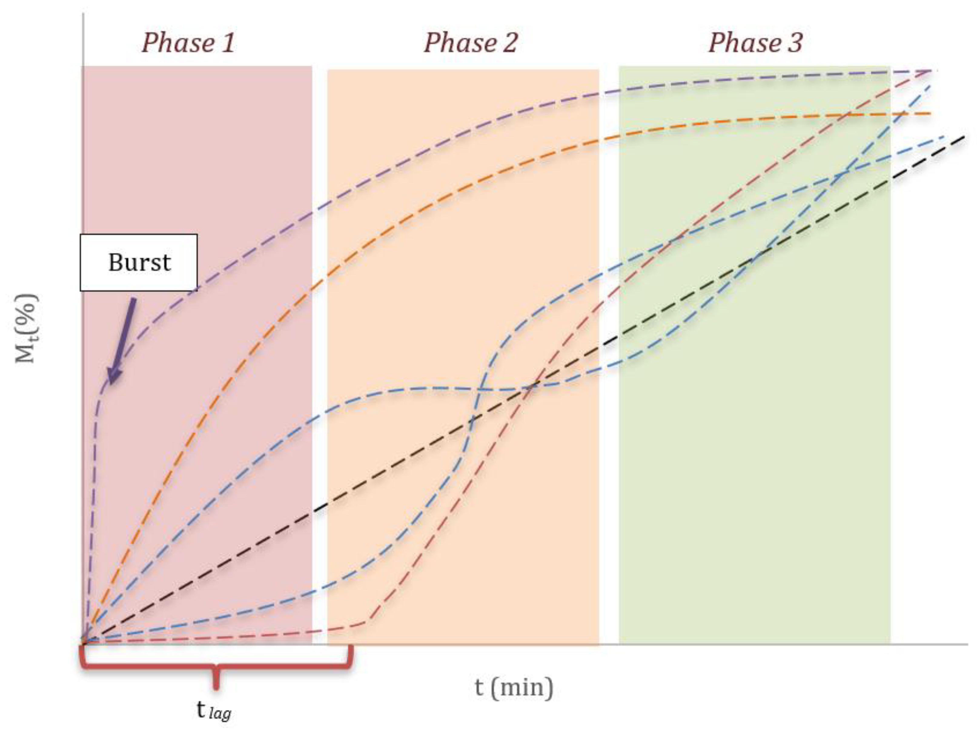
Release systems can exhibit dissolution profiles governed by different mechanisms, such as matrix swelling, polymer chain relaxation, erosion or disintegration of the system, which can be manifested in differentiated phases [
5]. As illustrated in
Figure 1, it is possible to distinguish three characteristic stages: an initial phase (Phase 1), where a lag time (t
lag) or a sudden release phenomenon (Burst) can occur; an intermediate phase (Phase 2), in which a release mechanism associated with the kinetics of the system predominates; and a final phase (Phase 3), with the curve approaching a plateau and reflecting the depletion of the available drug. The diversity of possible trajectories highlights the importance of selecting an appropriate mathematical model to describe a specific profile.
Classical dissolution models assume that the release of the API begins immediately upon contact with the dissolution medium. However, in various pharmaceutical forms, this process is observed to begin after an interval of no apparent release, known as lag time (tlag). Since most kinetic models do not explicitly consider this delay, it can be incorporated by simply modifying the fitting function over time. In this approach, M(t)=0 is assumed for t<tlag, and release follows the selected equation from that time, shifting the time variable to M(t)=M(t− tlag).
In certain cases, the initial process is characterized by an abrupt increase in release, known as the burst effect, usually caused by the rapid release of the drug from the DDS surface. This leads to the fact that at times close to 0, a certain amount of drug may already be found dissolved, so this behavior can be expressed as M
Burst(t)=M(t) + b, where b is the amount of drug dissolved at the start of the test [
27].
In other cases, a change in the type of process governing drug release can be observed, resulting in complex profiles that typically have an inflection point at a time called ti, which marks the change in the phenomenon. That is, from t=0 to t=ti, the profile can be described by a M1(t) model, while from t=ti, the curve is fitted with another M2(t) model.
2.2. Parameters of Pharmaceutical Relevance
Drug release profiles can be characterized using various parameters, both from a theoretical and practical perspective. The main parameters of pharmaceutical relevance are described below, explaining their physical significance and application in immediate, extended, or dual-release systems.
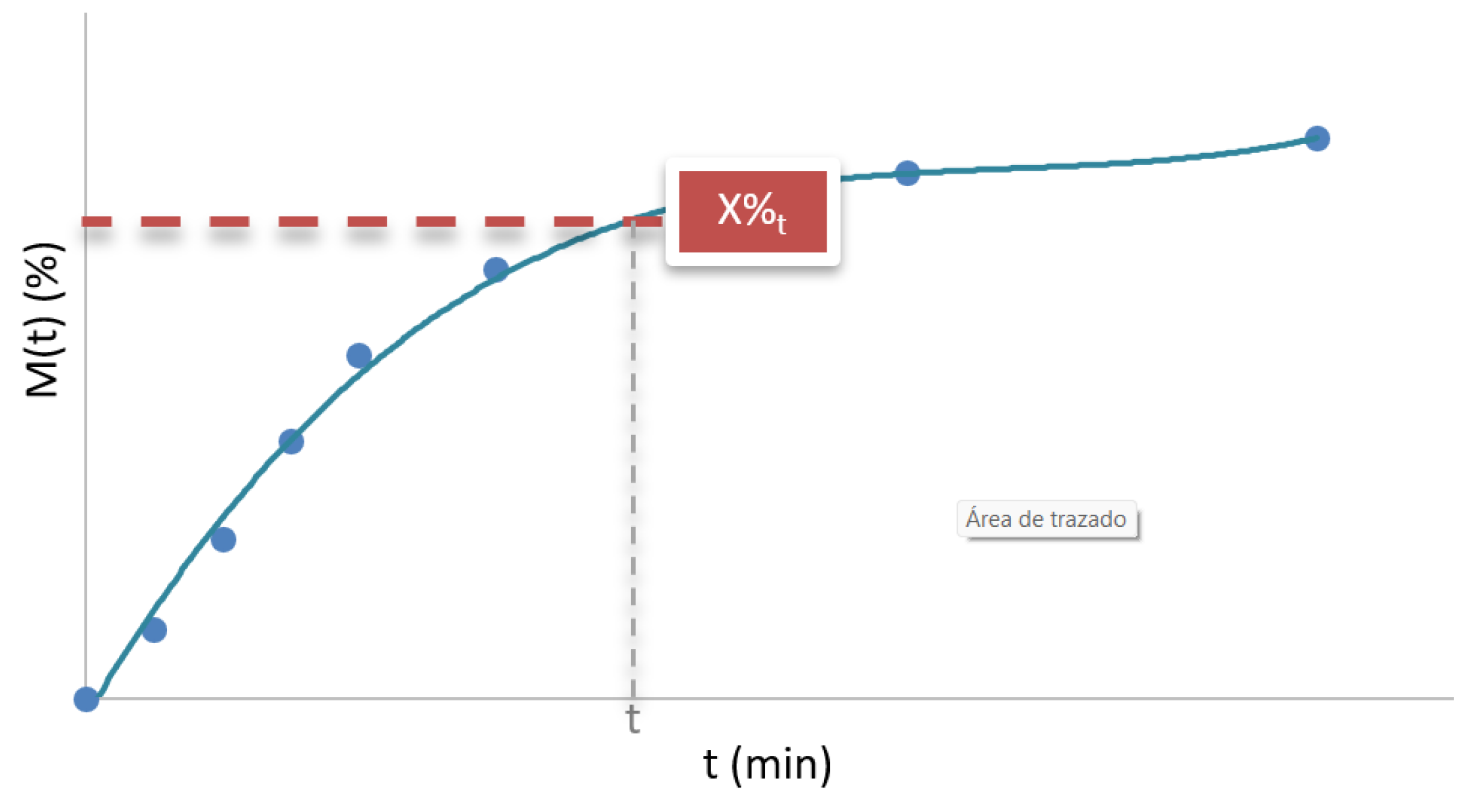
2.2.1. Drug Released at a Given Time
The drug released at a given time, represented as X%
t, corresponds to the cumulative percentage of the API released at a specific time t (
Figure 2) [
28]. This parameter determines what fraction of the drug has been dissolved in the release medium up to that point. For example, if X%
30min=75% is reported, this means that 75% of the total drug contained in the formulation has been released 30 minutes after the test began.
From a practical perspective, X%t is especially useful for comparing formulations with criteria established by pharmacopoeias or regulatory standards, since many of them specify minimum percentages that must be achieved within certain times. It also provides relevant information on the release rate, which is essential in formulations requiring rapid action of the API.
The interpretation of this parameter depends on the type of release system. In immediate-release formulations, X%t values are usually high even for low values of time, reflecting rapid dissolution of the API. In contrast, in sustained-release systems, a slower release is observed, with lower X%t values at the beginning of the profile, since the design seeks to extend the availability of the drug over time. Dual-release systems, on the other hand, combine both behaviors: a fraction of the active ingredient is released rapidly at the beginning, followed by a second phase of sustained release, resulting in a profile with an abrupt initial increase and a gentler slope thereafter.
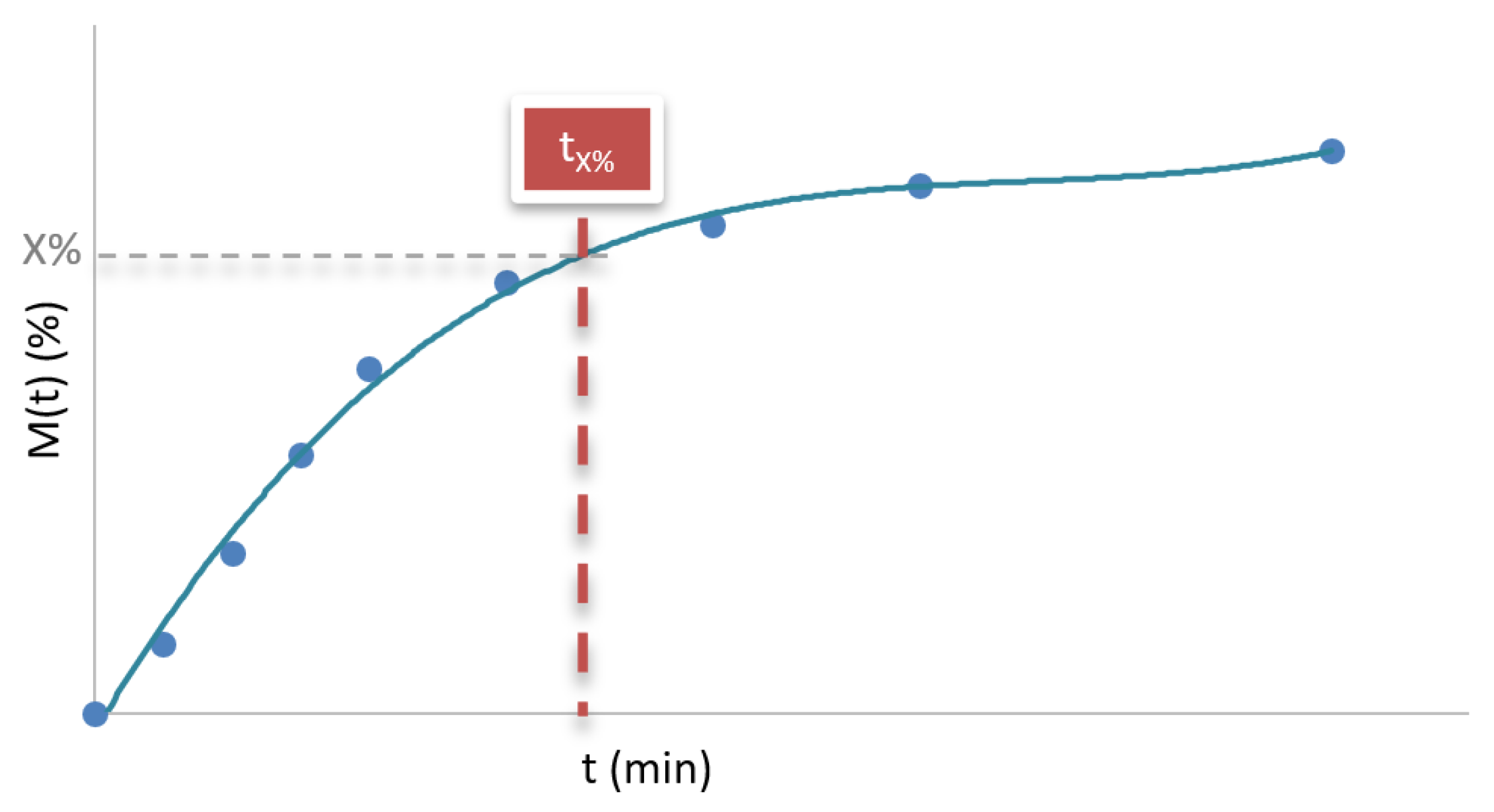
2.2.2. Time Required to Release a Percentage of the Drug
The time required to release a given percentage of the drug, represented as t
X%, corresponds to the time at which a specific cumulative percentage of the API has been released (
Figure 3) [
3]. This parameter reflects how much time has elapsed from the start of the assay until, for example, 50% (t
50%) or 80% (t
80%) of the total drug content in the formulation has been released. Thus, if a t
80% of 45 minutes is informed, it means that the formulation requires 45 minutes to release 80% of the API.
This value is especially relevant because it constitutes a direct indicator of the overall rate of the release process; the lower the tX%, the faster the drug release. Therefore, it is a useful parameter both in the development of formulations and in the comparison of dissolution profiles, allowing for an assessment of whether a system is suitable for a rapid or a sustained therapeutic action.
The interpretation of tX% also depends on the type of delivery system. In immediate-release formulations, tX% values are usually low, as the goal is for the drug to be available in the body as soon as possible. In contrast, in sustained-release formulations, tX% is considerably higher, reflecting delayed and controlled dissolution.
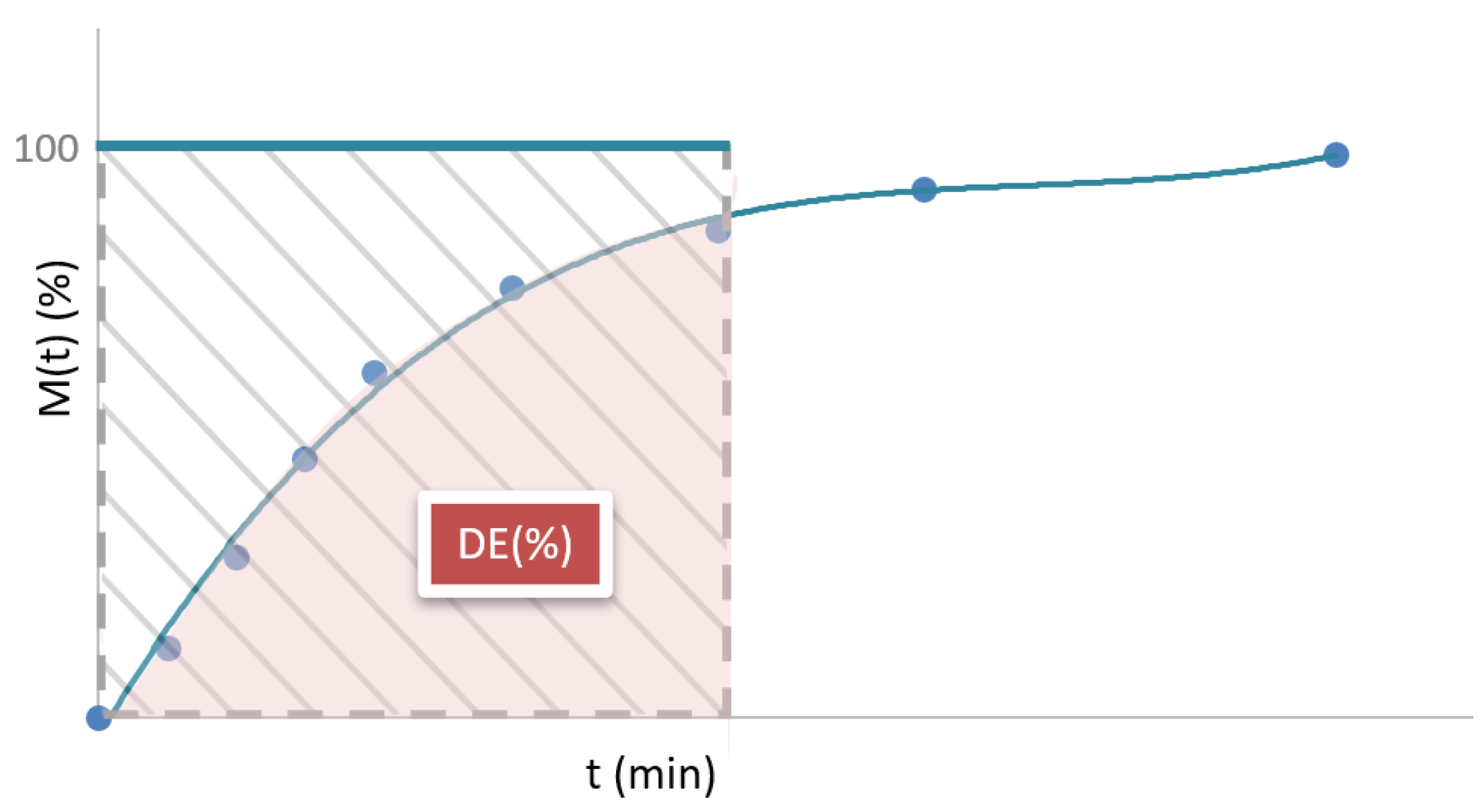
2.2.3. Dissolution Efficiency
Dissolution efficiency, abbreviated as DE
t, is a parameter that quantifies the overall efficiency of the drug release process within a given time interval. It is defined as the ratio of the area under the dissolution curve (cumulative release profile) up to a certain time t
j, expressed as a percentage of the area of the rectangle described by 100% release in the same time (
Figure 4). The corresponding mathematical expression is shown in Equation 1 [
29,
30,
31].
where
M(t) represents the amount of drug dissolved as a function of time.
From a physical perspective, DEt allows estimating the release efficiency of the API over the analyzed time interval. Unlike specific parameters such as tX% or X%t, DEt considers the release curve, integrating information on the rate and quantity released over time. Therefore, it is a value that reflects the overall behavior of the release system and allows for quantitative comparisons between different formulations.
This parameter can take different values depending on the time interval chosen for its calculation. For this reason, it is essential to define a time t
j that is representative of the behavior of the formulation. In practice, it is recommended that t
j cover at least 90% of the API release, to consider most of the dissolution profile, although this is not always appropriate in very slow-release formulations [
29]. In immediate-release systems, DE
t is usually high, close to 100%, since most of the drug is released rapidly. In sustained-release formulations, DE
t tends to be lower in the initial stages. In dual-release systems, DE
t can reach intermediate or high values, depending on the ratio of the immediate-release fraction to the extended-release phase.
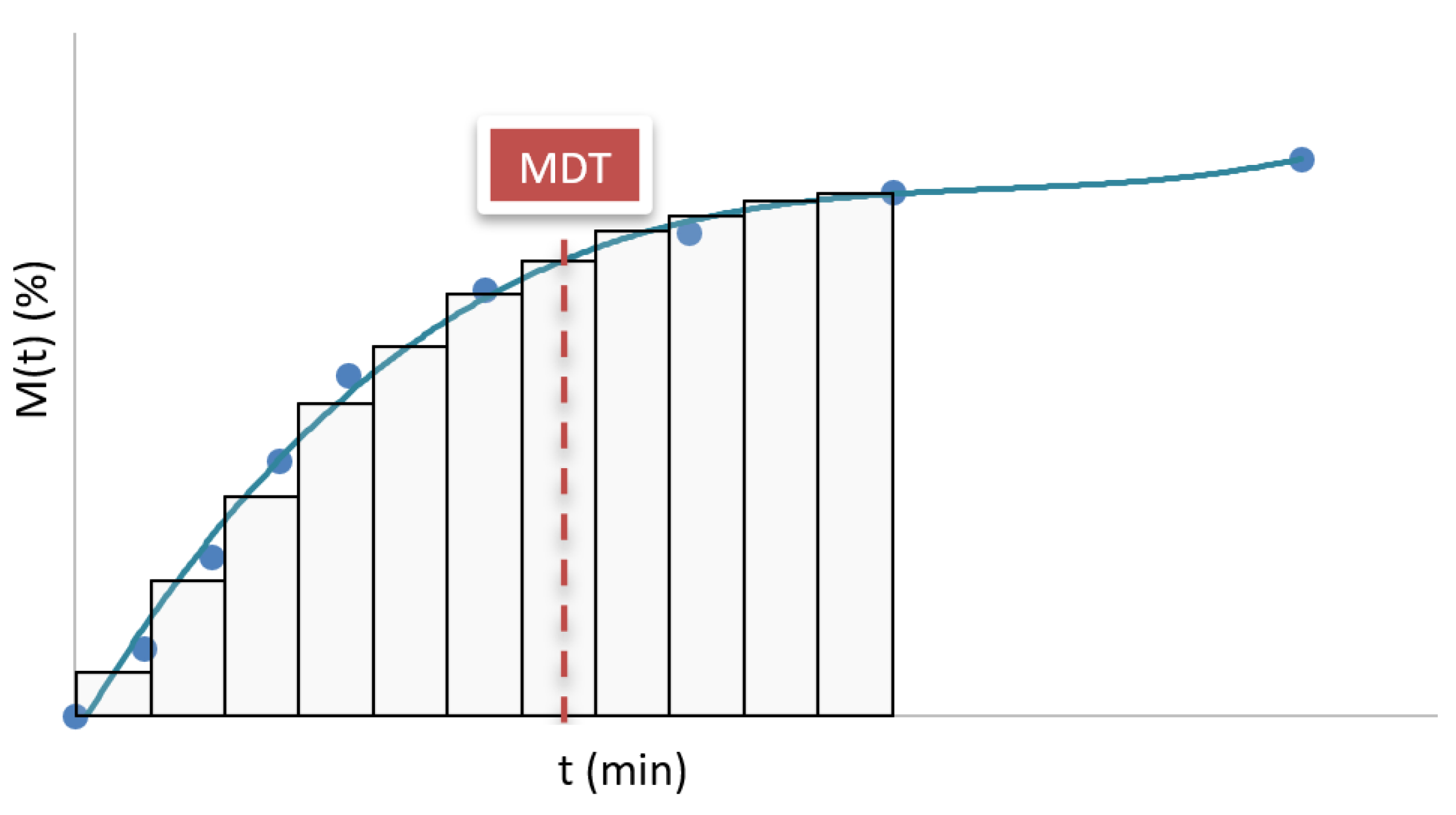
2.2.4. Mean Dissolution Time
The mean dissolution time (MDT
X%) is a parameter that expresses the average time in which the API is released throughout the dissolution process (
Figure 5). This value summarizes the temporal distribution of drug release, providing a more comprehensive view of the dissolution profile than the parameter t
X% [
32].
From an experimental perspective, the MDT
X% is calculated using model-independent statistical methods based on data obtained from the dissolution test. One of the most commonly used expressions for its determination is shown in Equation 2 [
30,
31,
33].
where
and represents the midpoint between two consecutive sampling times, and Δ
M% is the percentage increase in drug released between those two points.
This parameter is very useful in the comparative characterization of formulations, as it provides a quantitative estimate of the overall release rate. A low MDTX% indicates that most of the API is released rapidly, while a high value suggests a slower and more sustained release.
It is important to note that the MDTX% value can be influenced by the time range chosen for its determination. If the time interval considered includes phases in which drug release is minimal or practically zero (for example, when the curve flattens), these late points can distort the average, raising the MDTX% beyond the interval in which most of the release occurred. Therefore, in many cases, this parameter is calculated until a specific cumulative release percentage is reached, such as MDT80%. This choice must be aligned with the objective of the analysis and the type of formulation evaluated, to ensure that the MDT faithfully represents the active release phase.
In immediate-release systems, MDT is usually low, typically less than 20 minutes, reflecting the rapid availability of the API. In extended-release formulations, the MDT is considerably longer and can reach several hours depending on the system design and the polymer or matrix used. In the case of dual-release formulations, the MDT value represents an average of both phases.
2.3. Pharmaceutical Systems for Algorithm Validation
To validate the proposed decision tree, four DDSs were selected, each with different release mechanisms and experimental conditions, to cover various scenarios, from predominantly diffusive releases to systems with mixed or erosion-controlled mechanisms. Their characteristics, formulation, and test conditions are briefly described below. In all cases, the tests were performed in triplicate.
2.3.1. Case Study A—Hydrogels
The first system to be analyzed consists of poloxamer-based thermoreversible hydrogels loaded with ivermectin (IVM), classified under the Biopharmaceutical Classification System (BCS) as a Class II drug. The hydrogels were prepared by an adaptation of the cold method described by Romero [
28]. For the analysis, the profiles of the systems loaded with IVM at concentrations of 0.5% w/w (A1), 1.0% w/w (A2), and 1.5% w/w (A3) were selected. IVM release assays from the hydrogels were performed in a modified Franz cell with two compartments separated by a dialysis membrane. Physiological solution (0.9% NaCl) was used as the dissolution medium, and at predetermined time intervals, the medium was completely replaced with fresh medium.
2.3.2. Case Study B—Films
The second system to be analyzed is poly(3-hydroxybutyrate) (PHB) films loaded with dexamethasone (DX), chosen to represent prolonged release formulations in which the process is controlled by diffusion and no visible erosion of the matrix is observed. The systems selected for the decision tree application contained DX concentrations of 6% w/w (B1), 21% w/w (B2), and 29% w/w (B3).
In vitro assays were carried out by placing a 1 × 1 cm² square submerged in 3 ml of saline solution with complete removal of the medium [
34].
2.3.3. Case Study C—Dome Matrix
The Dome Matrix systems were prepared with mixtures of hydroxypropyl methylcellulose (HPMC) K15M and HPMC K100LV, incorporating 10% riboflavin (RF) and presenting a dome-type geometry. The ratios of the HPMC K15M/HPMC K100LV polymers used (in mg) were 10/30 (C1), 20/20 (C2), and 30/10 (C3). RF release assays were performed in a USP II dissolution apparatus using simulated gastric fluid without pepsin [
35].
2.3.4. Case Study D—3D-Printed Tablets
The latest case study involves 3D-printed tablets composed of Gelucire® 50/13 and loaded with 10% w/w IVM. An oblong geometry with a flat surface and a reticulated internal structure was designed. To evaluate the decision tree, the profiles of three formulations with different dimensions were analyzed: the first with a semi-major axis of 18 mm, a semi-minor axis of 10 mm, and a thickness of 6 mm (D1), and the remaining formulations with a size that decreased proportionally in all three axes by 10% (D2) and 30% (D3) relative to D1. The
in vitro release profiles were determined in a type II dissolution apparatus, using 0.1 N HCl as the dissolution medium [
36].
3. Results
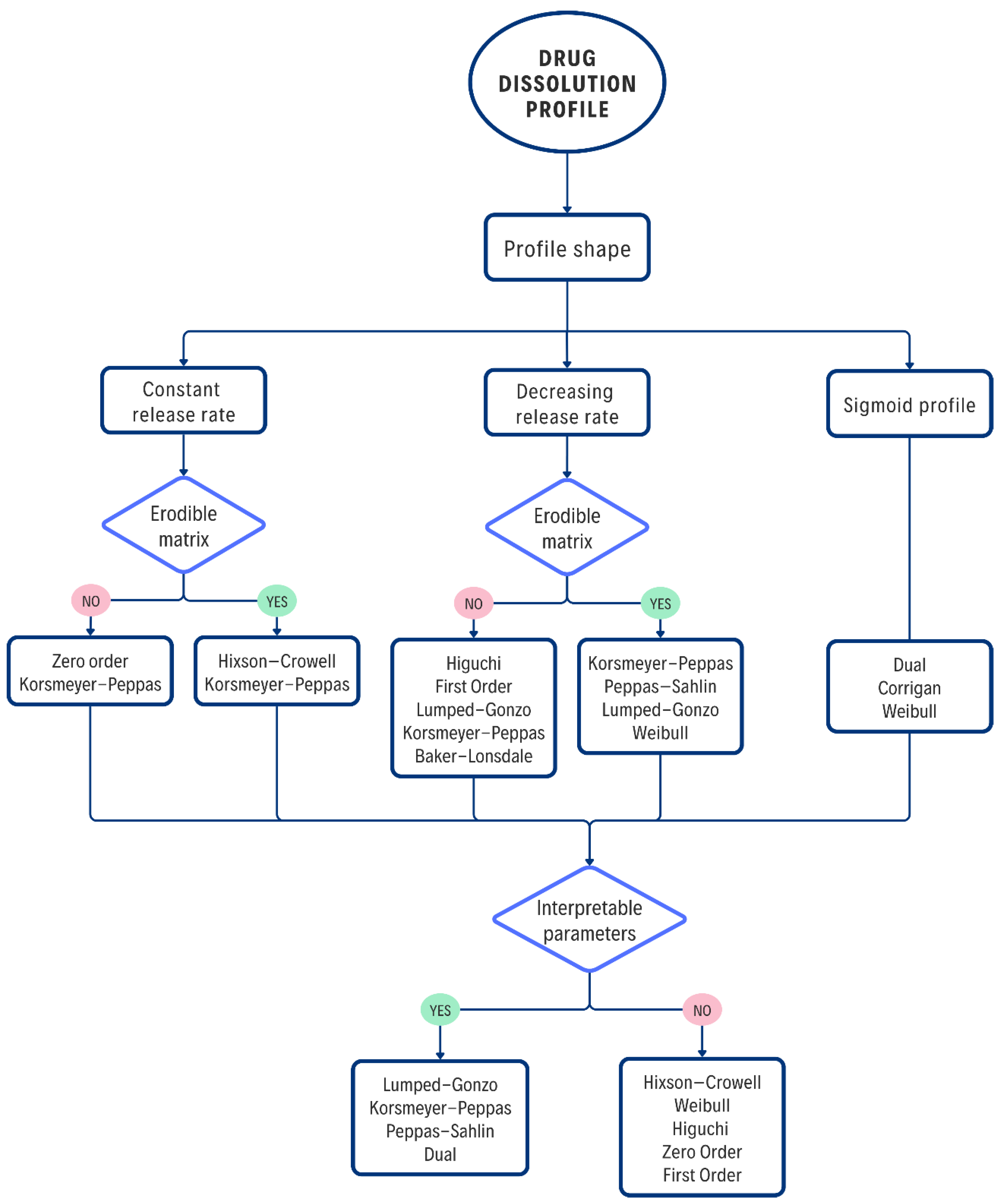
3.1. Decision Tree
The proposed decision tree (
Figure 6) is not intended to replace the researcher's experience, but rather to offer a logical and structured framework to guide the selection of mathematical models for the analysis of results obtained in
in vitro studies. It begins with direct observation of the release profile and physical characteristics of the system and concludes with the selection of a model based not only on statistical fit but also on the ability of the model parameters to provide useful pharmaceutical or physical information.
First, it is proposed to classify the experimental curve according to its general shape—linear, with decreasing slope or sigmoid—since this first filter allows to limit the available options. It is also important to consider the complexity of the models, since linear profiles can also be described by Higuchi, Weibull or Lumped–Gonzo; however, these options are discarded at this stage due to their higher mathematical complexity without providing significant advantages in the fit. Observational criteria are then incorporated, such as the behavior of the dosage form during the in vitro assay, which help infer the predominant mechanism. For example, variations in the geometry and dimensions of the DDSs, or the presence of suspended particles in the dissolution medium, can be detected. These observations allow for the elimination of some options; however, it is recommended that the researcher verify that the system complies with the restrictions imposed on each model.
The selection process culminates with a key decision: whether the chosen model allows obtaining parameters with interpretive value for the design or understanding of the system. When the purpose of the study includes understanding the mechanism or adjusting critical variables, models such as K-P, Peppas–Sahlin (P-S), or L-G are prioritized. However, if the objective is simply to achieve a good predictive fit, more empirical or general models, such as W or FO, can be used. The physical interpretation of kinetic parameters provides valuable information for the design, optimization, and scaling of formulations, as well as for supporting, before regulatory agencies, the robustness of the release system's performance in various environments.
3.2. Validación del Árbol de Decisión
3.2.1. Case Study A—Hydrogels
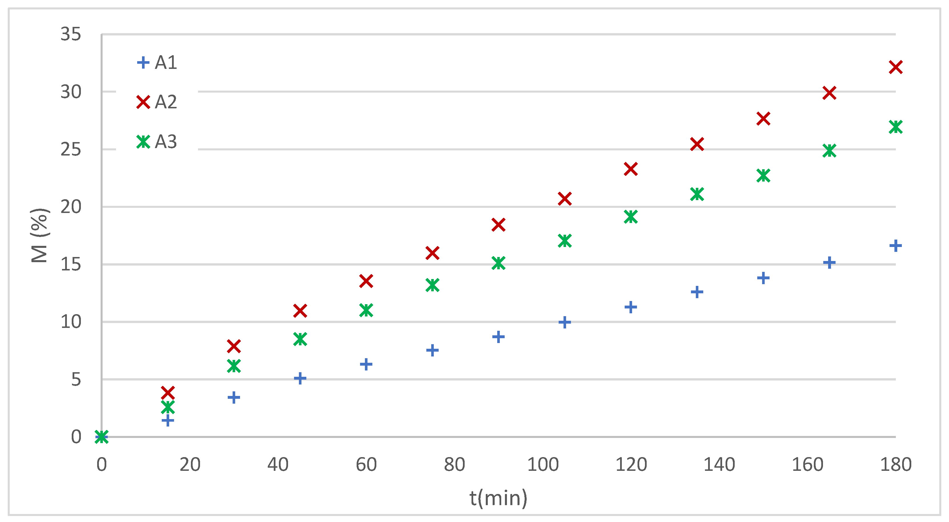
The experimentally obtained dissolution profiles of IVM from thermoreversible hydrogels are shown in
Figure 7.
The analysis of these profiles showed a clear linear trend. Furthermore, considering that the system was evaluated in a modified Franz cell with a membrane barrier, it was initially assumed that diffusion is the predominant phenomenon in the test. This led to the selection of two possible models: K-P and zero-order (Z-O).
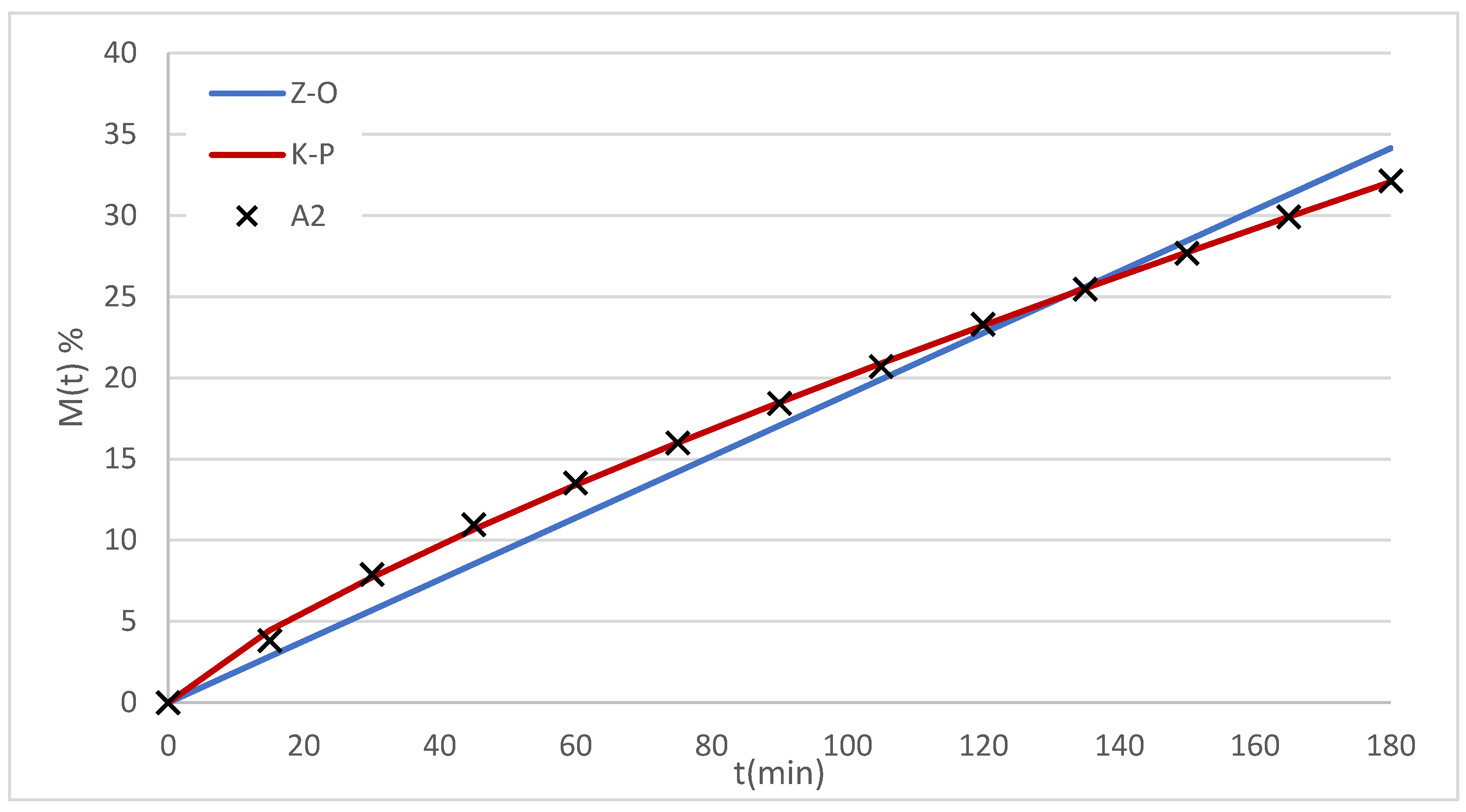
The data were fitted with both models (
Figure 8) and the obtained parameters are summarized in
Table 2. Comparison criteria included R
2, AIC and residual analysis.
In all cases, both models fitted the data satisfactorily, although K-P showed lower AIC values and better R2. Furthermore, the model's exponent n ranged between 0.79 and 0.89, corresponding to a non-Fickian transport regime.
Table 3 presents parameters of pharmaceutical interest calculated with both models.
The results show that K-P is more sensitive than the zero-order model, since it reflects the differences between systems A1–A3 with greater variation.
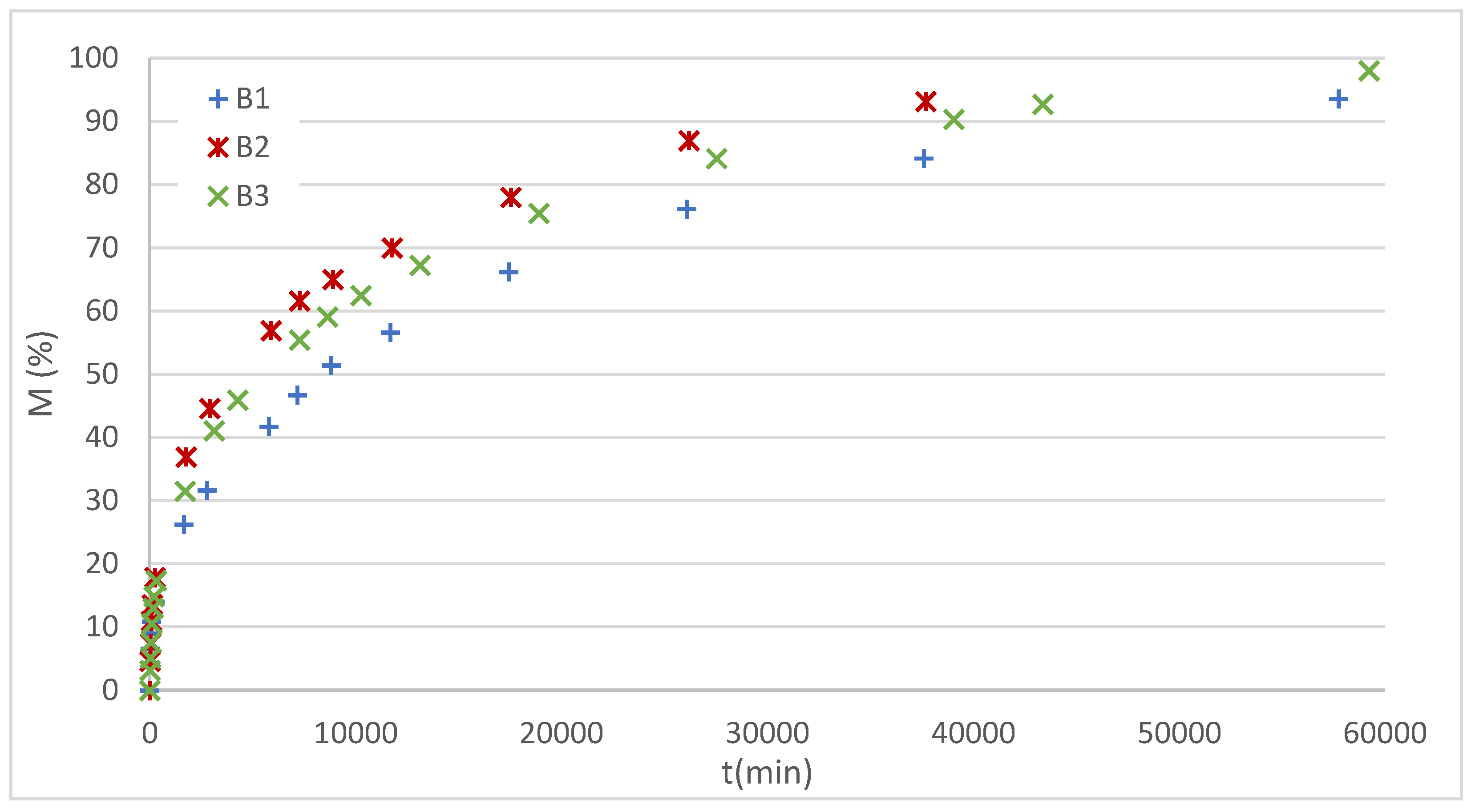
3.2.2. Case Study B—Films
The experimentally obtained dissolution profiles for the DX-loaded films are shown in
Figure 9.
The profiles of this study system exhibit a decreasing slope, corresponding to diffusion-controlled release processes. Furthermore, since no erosion was observed, the H, first order (FO), L-G, and K-P models were considered candidates. The Baker-Lonsdale model was discarded due to its geometric restrictions, which limit it to spherical systems.
Figure 10 shows the fitting of the B1 film profile with the selected models, while
Table 4 details the adjustment parameters obtained for the three films analyzed.
In all systems, the K-P and L-G models showed the best statistical indices, with R2 values greater than 0.99 and lower AIC values compared to H and FO. Analysis of the exponent n in K-P (0.35–0.42) indicates fickian transport, which is consistent with the initial hypothesis of dominant diffusion in the absence of membrane erosion. The L–G model satisfactorily described the entire release profile, also providing parameters with pharmacokinetic interpretation.
From the models, the pharmaceutical parameters of interest presented in
Table 5 were calculated.
It is important to clarify that the pharmaceutical parameters were calculated for all preselected models, except for the Power Law model, as this model can only be applied to describe 60% of the release. In contrast, the L-G model demonstrated the ability to fit the entire dissolution profile, in addition to allowing for the estimation of the initial release rate.
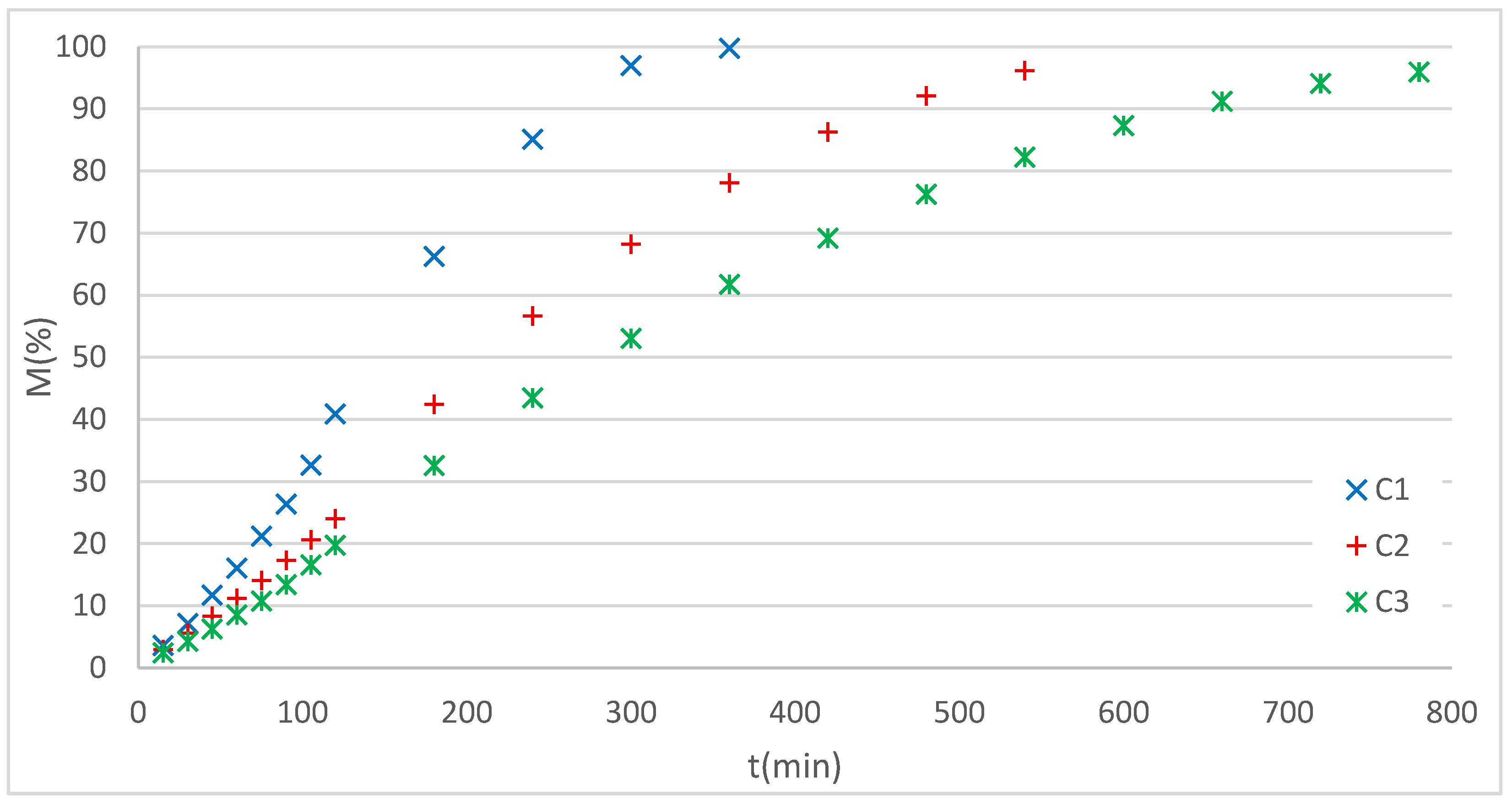
3.2.3. Case Study C—Dome Matrix
Figure 11 shows the RF dissolution profiles obtained experimentally from the dome matrices.
It can be observed that the RF release profiles in all cases correspond to sigmoidal or dual curves, indicating the presence of a composed release mechanism. For this pattern, the Gallagher–Corrigan, Dual, or W models could initially be used. However, the first was discarded because it applies to systems with a burst effect, a phenomenon not observed in the release profiles of these systems.
The data were therefore fitted using the Dual (K–P + L–G) and W models.
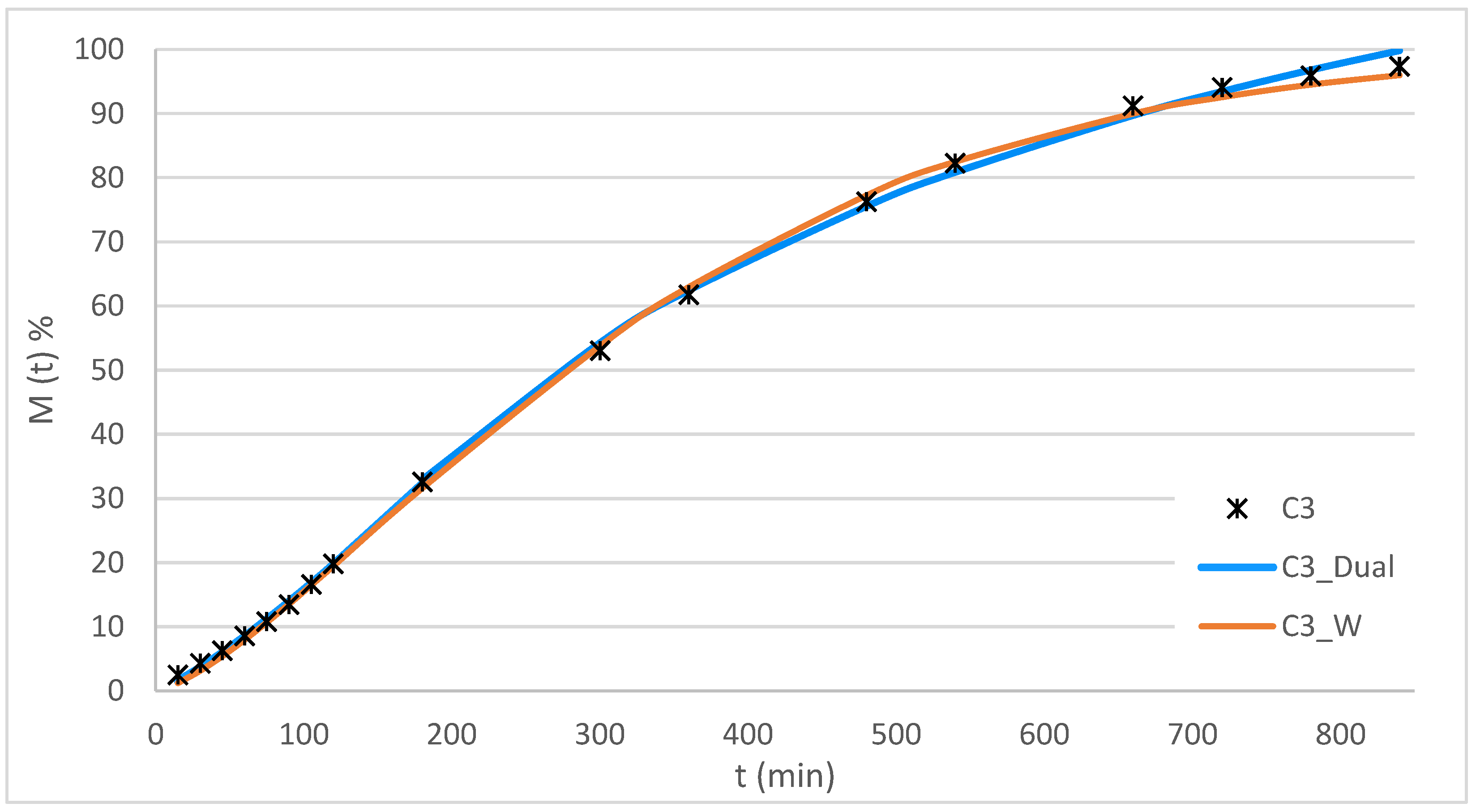
Figure 12 presents the experimental data for the C3 system along with the curves for the applied models, while
Table 6 summarizes the statistical fitting parameters for the three systems analyzed.
The results show that both models achieved excellent fits, with R2 values greater than 0.998 and very low AICs. The Dual model accurately described the release in two distinct phases, providing parameters associated with specific mechanisms: an initial stage governed by diffusion (K-P) and a second stage modeled by L-G. In contrast, the W model, although it showed a comparable fit, is an empirical model without a physical interpretation of the mechanism, which limits its usefulness in understanding the processes.
From the adjustments with both models, the pharmaceutical parameters were calculated (
Table 7).
The values of t80%, MDT80% and DE350min t80%, MDT80%, were very similar for both models, reinforcing the robustness of the fits. However, the ability to interpret the release mechanism gives the Dual model a decisive advantage over the W model.
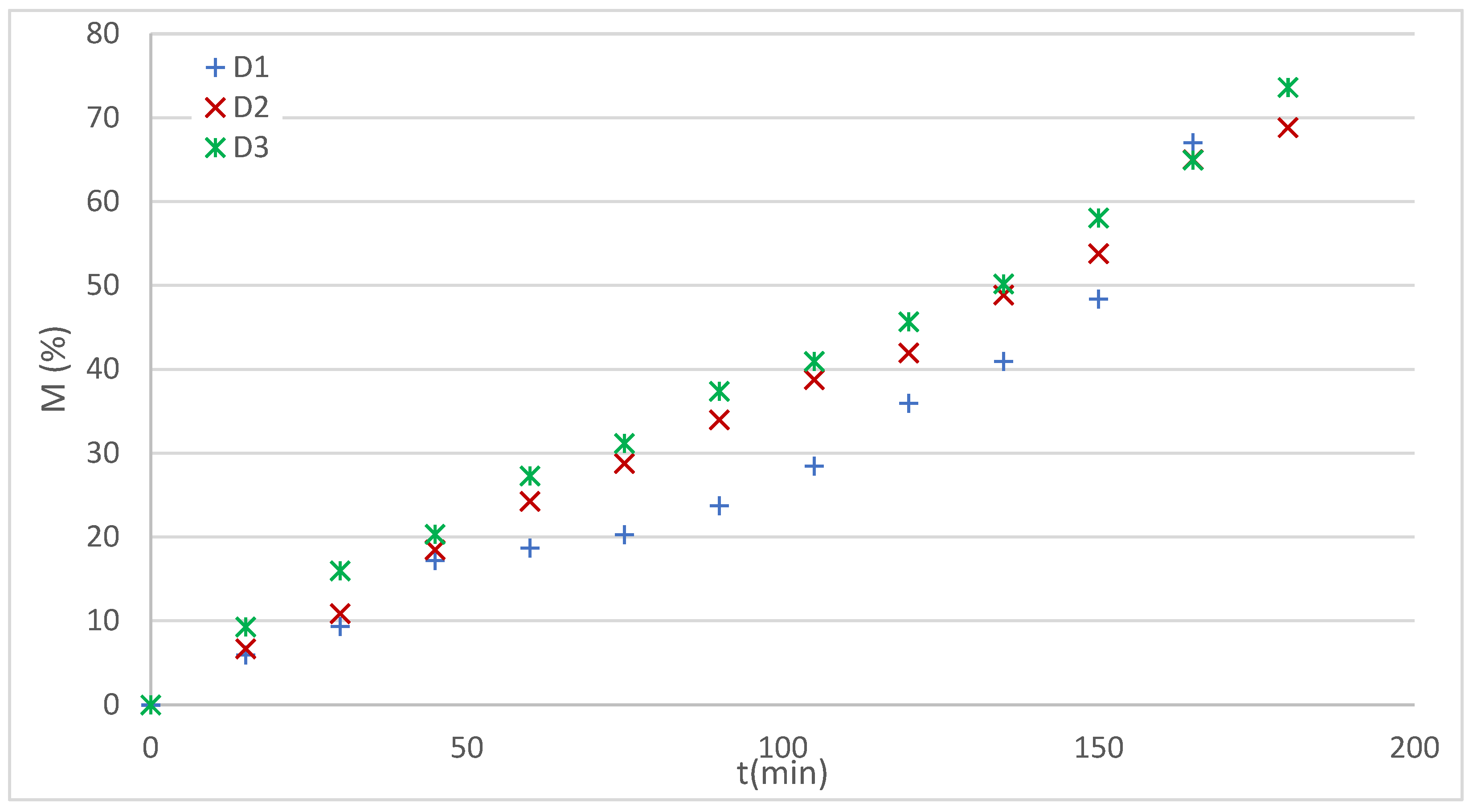
3.2.4. Case Study D—3D-Printed Tablets
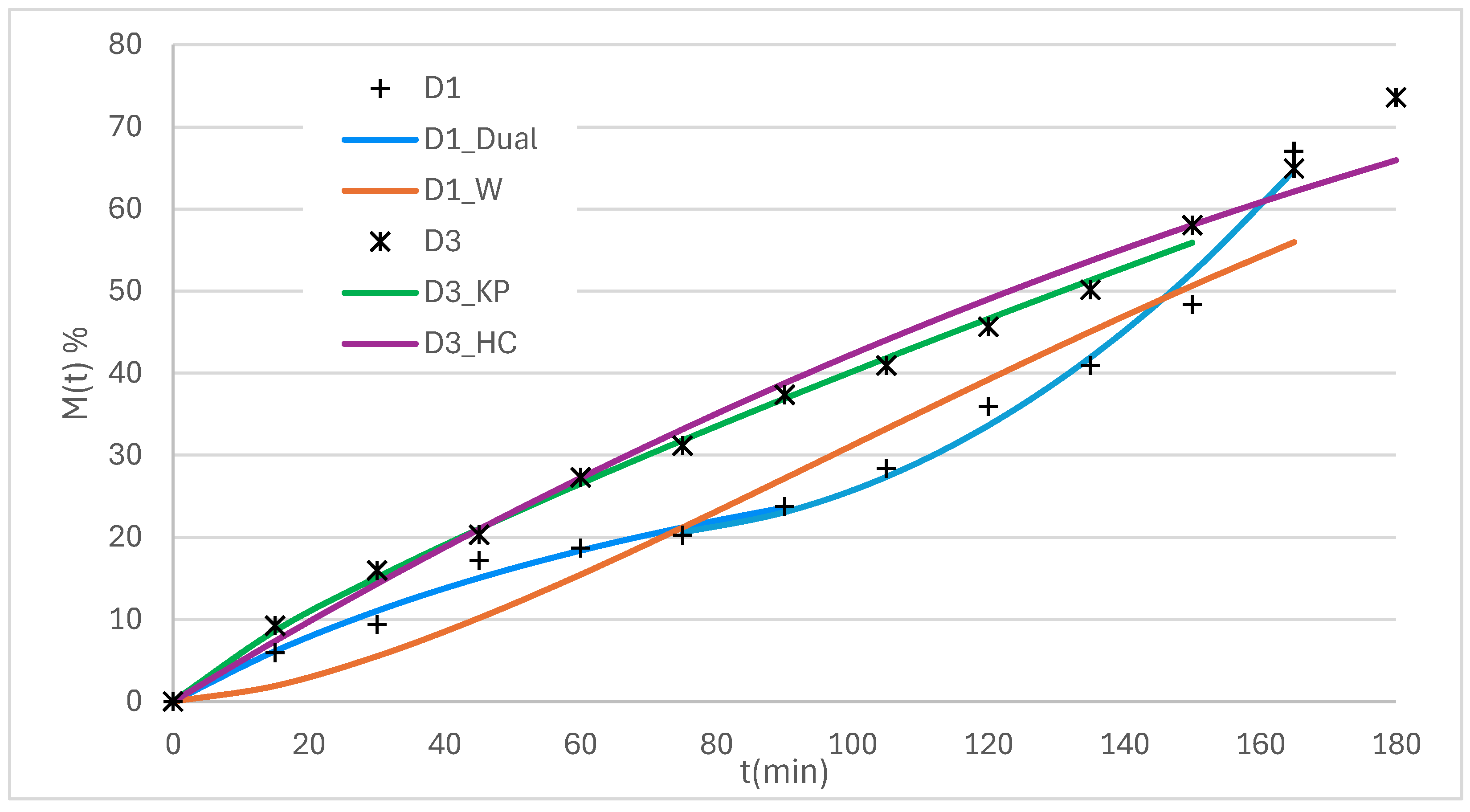
The experimental profiles obtained for the 3D printed systems are presented in
Figure 13.
The profiles of the systems D2 and D3 are observed to be approximately linear, while the profile of the D1 system is characterized by dual behavior.
For the analysis of D2 and D3 profiles, the Hixson and Crowell (H-C) and K-P models were applied following the sequence that applies to systems with erosion.
Figure 14 shows the experimental data for systems D1 and D3 together with the curves of the applied models, while
Table 8 summarizes the statistical adjustment parameters for the three systems analyzed.
En For systems D2 and D3, R2 values > 0.99 were achieved with both models, confirming an excellent fit. However, the K-P model offers a key advantage, as it allows obtaining a diffusion exponent interpretable in terms of the release mechanism.
In contrast, system D1 exhibited dual behavior. For this case, the Dual LG–KP model was applied, which combines an initial phase fitted with L–G (to describe the initial delay) and a subsequent phase with K–P (to account for acceleration upon release). This model achieved the best statistical fit, reflected in the R
2 and AIC values (
Table 9). The W model, although also applicable, showed inferior fit parameters, which was reflected in a lower descriptive power of the observed dynamics.
The parameters of pharmaceutical relevance calculated for each system are presented in
Table 9.
Values of t45%, MDT45% and DE150min were similar for all the models, which reinforces the solidity of the adjustments made.
4. Discussion
Validation of the proposed decision tree demonstrated its usefulness in real experimental scenarios, covering different release mechanisms and test conditions. Its application allowed reducing the number of candidate models and guiding the selection toward those that offer an adequate balance between mathematical simplicity, quality of fit, and interpretive capacity of the parameters. This aspect is relevant considering that the indiscriminate application of multiple models is common in literature, without prior evaluation of their relevance [
4,
7].
The approach starts from a key point: the initial observation of the experimental profile, which acts as the trigger for the algorithm. This initial look, although simple, provides critical information by allowing the curve to be classified into general categories (linear, decreasing, sigmoidal, or dual). This focusing is consistent with previous work, where the shape of the curve and the presence of phenomena such as burst or lag time are early indicators of the predominant mechanisms [
1,
3]. In this way, the algorithm integrates observational criteria with statistical adjustment parameters (R², AIC), differentiating itself from approaches based exclusively on quantitative metrics.
The results also confirm the tension between precision and applicability. Complex or semi-empirical models, such as L–G, can accurately describe complete profiles and provide parameters with physical meaning (e.g., initial release rate), while empirical models, such as W, are more versatile and easier to apply but lack mechanistic interpretation [
5]. This dichotomy requires considering the specific objectives of each study: exploratory characterization, comparative analysis between formulations, or rational design of advanced systems.
Another relevant contribution is that the algorithm is not intended to replace the researcher's experience, but rather to serve as a supporting tool that structures the selection process. In this sense, it is consistent with recent approaches that view mathematical modeling as an interpretive complement and not a substitute for experimental evidence [
6].
The performance of the L–G model is noteworthy: its ability to fit complete profiles positions it as a competitive alternative to classic models such as K–P or W. Furthermore, the results obtained with polymer matrices, modular systems, and solid forms manufactured by 3D printing demonstrate the versatility of the model, which was able to adapt to scenarios of varying complexity. This reinforces the idea that the method is applicable to a wide range of experimental situations, as long as its limitations are recognized.
Finally, the value of the decision tree also lies in its dynamic and flexible nature: it is not restricted to a fixed set of equations, but rather allows for the incorporation of new models as they are validated in the literature. This characteristic ensures the approach's validity and applicability in a constantly evolving field.
5. Conclusions
This work proposed and validated a decision tree algorithm to guide the selection of mathematical models for drug dissolution and release. The approach is based on the initial visual analysis of the experimental profile as the starting point for the selection process. From this initial observation, the algorithm guides toward plausible models based on the curve shape, the observed physicochemical phenomena, and each model's ability to provide parameters with pharmaceutical value.
The results show that the algorithm facilitates a rational and transparent selection, reducing the ambiguity that arises from the wide variety of available models. It also favors the use of simple yet robust models, without excluding the possibility of resorting to more complex equations when the purpose of the study requires obtaining additional interpretive parameters. In this way, a balance is achieved between practical applicability and scientific rigor.
The proposed methodology was also shown to be versatile and adaptable to different release systems, including hydrogels, polymer films, modular systems, and 3D-printed pellets. This diversity of cases reinforces the ability of the decision tree to be applied to experimental contexts with predominantly diffusive, erosive, mixed, or dual release mechanisms.
Finally, it is important to emphasize that the algorithm is not intended to replace the researcher's judgment, but rather to serve as a flexible and dynamic support tool, capable of incorporating new models as they are validated in the literature. In this sense, it represents a concrete contribution to promoting a more rational use of mathematical modeling in pharmaceutical research and development, combining efficiency, applicability, and scientific basis.
Author Contributions
Conceptualization, C.Ll. and C.B.; methodology, S.C.; formal analysis, A.C., E.G. and C.Ll.; investigation, C.B. and S.C.; writing—original draft preparation, S.C. and C.B; writing—review and editing, A.C., A.J. and J.B.; visualization, A.R. and M.V.; supervision, S.P. and J.R.; project administration, J.B. All authors have read and agreed to the published version of the manuscript.
Funding
This research received no external funding.
Institutional Review Board Statement
Not applicable.
Informed Consent Statement
Not applicable.
Data Availability Statement
The original contributions presented in this study are included in the article. Further inquiries can be directed to the corresponding authors.
Acknowledgments
Authors would like to thank to Félix Manuel Chagra, Marta Alicia Hoyos and José Victor Mleziva for organizing the collected scientific information.
Conflicts of Interest
The authors declare no conflicts of interest.
References
- Thomas, F. The Fundamentals of Dissolution Testing. Pharm. Technol. 2019, 43. [Google Scholar]
- Gregory, K. Webster, X.S., and Paul D. Curry, Jr. A Staged Approach to Pharmaceutical Dissolution Testing. In Poorly Soluble Drugs; Jenny Stanford Publishing: 2016.
- Costa, P.; Sousa Lobo, J.M. Modeling and comparison of dissolution profiles. Eur. J. Pharm. Sci. 2001, 13, 123–133. [Google Scholar] [CrossRef]
- Zhang, Y.; Huo, M.; Zhou, J.; Zou, A.; Li, W.; Yao, C.; Xie, S. DDSolver: an add-in program for modeling and comparison of drug dissolution profiles. Aaps j 2010, 12, 263–271. [Google Scholar] [CrossRef]
- Romero, A.I.; Villegas, M.; Cid, A.G.; Parentis, M.L.; Gonzo, E.E.; Bermúdez, J.M. Validation of kinetic modeling of progesterone release from polymeric membranes. Asian Journal of Pharmaceutical Sciences 2018, 13, 54–62. [Google Scholar] [CrossRef]
- Trucillo, P. Drug Carriers: A Review on the Most Used Mathematical Models for Drug Release. Processes 2022, 10, 1094. [Google Scholar] [CrossRef]
- Askarizadeh, M.; Esfandiari, N.; Honarvar, B.; Sajadian, S.A.; Azdarpour, A. Kinetic Modeling to Explain the Release of Medicine from Drug Delivery Systems. ChemBioEng Reviews 2023, 10. [Google Scholar] [CrossRef]
- Kamaly, N.; Yameen, B.; Wu, J.; Farokhzad, O.C. Degradable Controlled-Release Polymers and Polymeric Nanoparticles: Mechanisms of Controlling Drug Release. Chem. Rev. 2016, 116, 2602–2663. [Google Scholar] [CrossRef] [PubMed]
- Siepmann, J.; Peppas, N.A. Modeling of drug release from delivery systems based on hydroxypropyl methylcellulose (HPMC). Advanced Drug Delivery Reviews 2001, 48, 139–157. [Google Scholar] [CrossRef]
- 5 - Mathematical models of drug release. In Strategies to Modify the Drug Release from Pharmaceutical Systems, Bruschi, M.L., Ed.; Woodhead Publishing: 2015; pp. 63–86.
- Gibaldi, G.; Perrier, D. Pharmacokinetics 2nd edition Marcel Dekker Inc. New York, New York.
- Higuchi, T. Rate of Release of Medicaments from Ointment Bases Containing Drugs in Suspension. J. Pharm. Sci. 1961, 50, 874–875. [Google Scholar] [CrossRef]
- Higuchi, T. Mechanism of sustained-action medication. Theoretical analysis of rate of release of solid drugs dispersed in solid matrices. J. Pharm. Sci. 1963, 52, 1145–1149. [Google Scholar] [CrossRef]
- Korsmeyer, R.W.; Peppas, N.A. Effect of the morphology of hydrophilic polymeric matrices on the diffusion and release of water soluble drugs. J. Membr. Sci. 1981, 9, 211–227. [Google Scholar] [CrossRef]
- Korsmeyer, R.W.; Gurny, R.; Doelker, E.; Buri, P.; Peppas, N.A. Mechanisms of solute release from porous hydrophilic polymers. Int. J. Pharm. 1983, 15, 25–35. [Google Scholar] [CrossRef]
- Ritger, P.L.; Peppas, N.A. A simple equation for description of solute release I. Fickian and non-fickian release from non-swellable devices in the form of slabs, spheres, cylinders or discs. Journal of Controlled Release 1987, 5, 23–36. [Google Scholar] [CrossRef]
- Peppas, N.A.; Sahlin, J.J. A simple equation for the description of solute release. III. Coupling of diffusion and relaxation. Int. J. Pharm. 1989, 57, 169–172. [Google Scholar] [CrossRef]
- Hixson, A.W.; Crowell, J.H. Dependence of Reaction Velocity upon surface and Agitation. Ind. Eng. Chem. 1931, 23, 923–931. [Google Scholar] [CrossRef]
- Weibull, W. A statistical distribution function of wide applicability. Journal of applied mechanics 1951. [Google Scholar] [CrossRef]
- Langenbucher, F. Letters to the Editor: Linearization of dissolution rate curves by the Weibull distribution. Journal of Pharmacy and Pharmacology 1972, 24, 979–981. [Google Scholar] [CrossRef]
- Romero, A.I.; Bermudez, J.M.; Villegas, M.; Dib Ashur, M.F.; Parentis, M.L.; Gonzo, E.E. Modeling of Progesterone Release from Poly(3-Hydroxybutyrate) (PHB) Membranes. AAPS PharmSciTech 2016, 17, 898–906. [Google Scholar] [CrossRef] [PubMed]
- Shabestari, S.M.; Pourmadadi, M.; Abdouss, H.; Ghanbari, T.; Abdouss, M.; Rahdar, A.; Cambón, A.; Taboada, P. pH-responsive chitosan-sodium alginate nanocarriers for curcumin delivery against brain cancer. Colloids and Surfaces B: Biointerfaces 2025, 255, 114875. [Google Scholar] [CrossRef] [PubMed]
- Baker, R.W. Controlled release: mechanisms and rates. In Controlled release of biologically active agents, Tanquary, A.C., Ed.; Plenum Press: New York, 1974; pp. 15–71. [Google Scholar]
- Corrigan, O.I.; Li, X. Quantifying drug release from PLGA nanoparticulates. Eur. J. Pharm. Sci. 2009, 37, 477–485. [Google Scholar] [CrossRef]
- Tsirigotis-Maniecka, M.; Szyk-Warszyńska, L.; Maniecki, Ł.; Szczęsna, W.; Warszyński, P.; Wilk, K.A. Tailoring the composition of hydrogel particles for the controlled delivery of phytopharmaceuticals. Eur. Polym. J. 2021, 151, 110429. [Google Scholar] [CrossRef]
- Lamarra, J.; Calienni, M.N.; Rivero, S.; Pinotti, A. Electrospun nanofibers of poly(vinyl alcohol) and chitosan-based emulsions functionalized with cabreuva essential oil. Int. J. Biol. Macromol. 2020, 160, 307–318. [Google Scholar] [CrossRef]
- Huang, X.; Brazel, C.S. On the importance and mechanisms of burst release in matrix-controlled drug delivery systems. Journal of Controlled Release 2001, 73, 121–136. [Google Scholar] [CrossRef]
- Romero, A.I.; Cid, A.G.; Minetti, N.E.; Briones Nieva, C.A.; García Bustos, M.F.; Gonzo, E.E.; Villegas, M.; J, M.B. Sustained-release hydrogels of ivermectin as alternative systems to improve the treatment of cutaneous leishmaniasis. Ther. Deliv. 2020, 11, 779–790. [Google Scholar] [CrossRef] [PubMed]
- Khan, K.A. The concept of dissolution efficiency. Journal of Pharmacy and Pharmacology 1975, 27, 48–49. [Google Scholar] [CrossRef] [PubMed]
- Nep, E.I.; Asare-Addo, K.; Ghori, M.U.; Conway, B.R.; Smith, A.M. Starch-free grewia gum matrices: Compaction, swelling, erosion and drug release behaviour. Int. J. Pharm. 2015, 496, 689–698. [Google Scholar] [CrossRef]
- Al-Hamidi, H.; Asare-Addo, K.; Desai, S.; Kitson, M.; Nokhodchi, A. The dissolution and solid-state behaviours of coground ibuprofen–glucosamine HCl. Drug Development and Industrial Pharmacy 2015, 41, 1682–1692. [Google Scholar] [CrossRef]
- Pillay, V.; Fassihi, R. Evaluation and comparison of dissolution data derived from different modified release dosage forms: an alternative method. J. Control. Release 1998, 55, 45–55. [Google Scholar] [CrossRef]
- Dugar, R.P.; Gajera, B.Y.; Dave, R.H. Fusion Method for Solubility and Dissolution Rate Enhancement of Ibuprofen Using Block Copolymer Poloxamer 407. AAPS PharmSciTech 2016, 17, 1428–1440. [Google Scholar] [CrossRef]
- Villegas, M.; Cid, A.G.; Briones, C.A.; Romero, A.I.; Pistán, F.A.; Gonzo, E.E.; Gottifredi, J.C.; Bermúdez, J.M. Films based on the biopolymer poly(3-hydroxybutyrate) as platforms for the controlled release of dexamethasone. Saudi Pharmaceutical Journal 2019, 27, 694–701. [Google Scholar] [CrossRef] [PubMed]
- Cid, A.G.; Sonvico, F.; Bettini, R.; Colombo, P.; Gonzo, E.; Jimenez-Kairuz, A.F.; Bermúdez, J.M. Evaluation of the Drug Release Kinetics in Assembled Modular Systems Based on the Dome Matrix Technology. J. Pharm. Sci. 2020, 109, 2819–2826. [Google Scholar] [CrossRef] [PubMed]
- Briones Nieva, C.A.; Real, J.P.; Campos, S.N.; Romero, A.I.; Villegas, M.; Gonzo, E.E.; Bermúdez, J.M.; Palma, S.D.; Cid, A.G. Modeling and evaluation of ivermectin release kinetics from 3D-printed tablets. Ther. Deliv. 2024, 15, 845–858. [Google Scholar] [CrossRef] [PubMed]
Figure 1.
Release profile types: linear profile (black curve); downward slope profile (orange curve); sigmoid profiles (blue curves); profile with lag time (red curve); profile with burst effect (violet curve).
Figure 1.
Release profile types: linear profile (black curve); downward slope profile (orange curve); sigmoid profiles (blue curves); profile with lag time (red curve); profile with burst effect (violet curve).
Figure 2.
Drug released at a given time (X%t).
Figure 2.
Drug released at a given time (X%t).
Figure 3.
Time required to release a certain percentage of the drug (tX%).
Figure 3.
Time required to release a certain percentage of the drug (tX%).
Figure 4.
Dissolution efficiency (DE).
Figure 4.
Dissolution efficiency (DE).
Figure 5.
Mean dissolution time (MDT).
Figure 5.
Mean dissolution time (MDT).
Figure 7.
IVM release profiles from poloxamer hydrogels.
Figure 7.
IVM release profiles from poloxamer hydrogels.
Figure 8.
Dissolution profiles for system A2 modeled with K-P and Z-O.
Figure 8.
Dissolution profiles for system A2 modeled with K-P and Z-O.
Figure 9.
DX release profiles from PHB films.
Figure 9.
DX release profiles from PHB films.
Figure 10.
Dissolution profile for B1 system adjusted with H, FO, L-G and K-P models.
Figure 10.
Dissolution profile for B1 system adjusted with H, FO, L-G and K-P models.
Figure 11.
RF release profiles from Dome Matrix systems.
Figure 11.
RF release profiles from Dome Matrix systems.
Figure 12.
C3 system profile fitted with Dual and W models.
Figure 12.
C3 system profile fitted with Dual and W models.
Figure 13.
IVM release profiles from 3D-printed tablets.
Figure 13.
IVM release profiles from 3D-printed tablets.
Figure 14.
D1 and D3 systems profiles fitted with Dual and W models and K-P and H-C models respectively.
Figure 14.
D1 and D3 systems profiles fitted with Dual and W models and K-P and H-C models respectively.
Table 1.
Comparison of mathematical models for drug release profiles.
Table 1.
Comparison of mathematical models for drug release profiles.
| Model |
Equation |
Parameters |
Application |
Advantages |
Restrictions |
Ref |
| Zero order |
|
: constant |
Constant release rate over time
Large amount of drug in the matrix |
Simple
Useful for systems with constant release (e.g., osmotic pumps) |
Constant area: no erosion or swelling |
[10] |
| First order |
|
: constant |
Release rate proportional to the remaining drug |
Applicable to simple pharmaceutical forms. Used in the release of soluble drugs from porous matrices. |
There are no phenomena of erosion or swelling. |
[11] |
| Higuchi |
|
D: diffusion coefficient of the drug in the matrix
A: amount of drug in the matrix
Cs: solubility of the drug in the matrix |
One-dimensional diffusion from a homogeneous matrix
D constant |
Classic model useful in flat matrix systems |
It is not intended for highly porous matrices, erosion phenomena, swelling, or changes in geometry |
[12,13] |
| Korsmeyer–Peppas |
|
a: constant
n: exponential constant related to the type of mechanism |
Applicable to a wide variety of systems with different geometries |
n allows the predominant release mechanism to be interpreted.
It can be used for different geometries. |
Valid up to 60% of the release.
The system must be understood in order to interpret n, as it varies with geometry.
The interpretation of k and n may change. |
[14,15,16]
|
| Peppas–Sahlin |
|
k1: Fickian diffusion kinetic constant
k2: kinetic constant due to relaxation effect
m: diffusional exponent |
Superposition of Fickian diffusion and polymer relaxation. |
Allows separation of contributions from diffusion and relaxation |
Parameters must be physically consistent
Originally used up to a disolved fraction of 80% |
[17] |
| Hixson and Crowell |
|
k: constant |
Systems where the dimensions vary, but not the shape.
Equal dissolution rate over the entire surface |
Suitable when there is geometric changes and erosion.
Can be applied to particulate systems of uniform sizes.
Can model non-erodible systems. |
The matrix should not change its shape significantly (this generally occurs up to 75–85% of dissolution).
It does not consider matrix partitioning or swelling. |
[18] |
| Weibull |
|
a: temporal parameter
b: shape parameter
: lag time |
Flexible statistical model (empirical fit)
Does not take into account phenomena that may occur |
Excellent fit in many cases, for sigmoid types |
Does not provide mechanistic information
Parameters do not have clear physical meaning |
[19,20] |
| Lumped–Gonzo |
|
a, b : model parameters |
Overall second-order kinetics: the rate of release depends on the amount of drug remaining. |
Adjust the entire profile
Parameters with physical meanings
Applicable to various types of systems |
It takes into account several mechanisms, so it does not discriminate against specific mechanisms. |
[5,21] |
| Baker & Lonsdale |
|
: diffusion coefficient
: solubility of the drug in the matrix
: radius of the spherical matrix
: initial drug concentration in the matrix |
Spherical geometry
Non-porous matrix
Diffusion as the dominant mechanism |
Adjust the profile for the entire range
Parameters can be grouped into a single one |
Constant diffusion coefficient
Non-erodible matrix |
[22,23] |
| Corrigan |
|
: fraction of drug available for release at the surface
: time to reach maximum release speed.
k: velocity constant for maximum release speed
: release rate constant
|
Two-stage release. The first stage is burst release from the surface, and the second stage involves polymer degradation as the main effect
|
Allows complex sigmoid profiles to be worked on.
Clearly differentiates between the terms of the two stages of libration.
Application in biodegradable polymers in various systems (nano and microparticles, gels) |
Large number of parameters |
[24,25,26] |
Table 2.
Parámetros de ajuste y parámetros de los modelos para el sistema A.
Table 2.
Parámetros de ajuste y parámetros de los modelos para el sistema A.
| Systems |
Models |
R2 |
R2adjusted |
AIC |
Parameters |
| A1 |
Z-O |
0.9984 |
0.9984 |
-0.5446 |
a=0.0583 |
| K-P |
0.9994 |
0.9994 |
-20.6930 |
a=0.0985
n=0.8930 |
| A2 |
Z-O |
0.9963 |
0.9963 |
11.5175 |
a=0.0615 |
| K-P |
0.9995 |
0.9994 |
-21.3945 |
a=0.1392
n=0.8329 |
| A3 |
Z-O |
0.9953 |
0.9953 |
22.3936 |
a=0.0773 |
| K-P |
0.9998 |
0.9997 |
-26.5760 |
a=0.2106
n=0.7948 |
Table 3.
Parameters of pharmaceutical relevance for case study A.
Table 3.
Parameters of pharmaceutical relevance for case study A.
| Systems |
Models |
t10% (min) |
DE120min (%) |
MDT10% (min) |
| A1 |
Z-O |
171.50 |
3.50 |
85.00 |
| K-P |
176.64 |
3.74 |
82.55 |
| A2 |
Z-O |
162.67 |
3.68 |
42.20 |
| K-P |
169.40 |
4.09 |
34.13 |
| A3 |
Z-O |
129.44 |
4.63 |
51.05 |
| K-P |
128.64 |
5.27 |
42.87 |
Table 4.
Adjustment and model parameters for case study B.
Table 4.
Adjustment and model parameters for case study B.
| Systems |
Models |
R2 |
R2adjusted |
AIC |
Parámetros |
| B1 |
H |
0.9867 |
0.9867 |
102.65 |
k=0.45746 |
| FO |
0.9896 |
0.9896 |
106.82 |
k=7.62x10⁻⁵
|
| L-G |
0.9912 |
0.9905 |
96.684 |
a=0.013
b=1.3x10⁻⁴
|
| K-P |
0.9979 |
0.9976 |
30.003 |
a=1.9103
n=0.3599 |
| B2 |
H |
0.9634 |
0.9634 |
125.47 |
k=2.66 x 10⁻⁵
|
| FO |
0.9861 |
0.9861 |
116.06 |
k=1.264 x 10⁻⁴ |
| L-G |
0.9924 |
0.9919 |
102.8 |
a=0.024
b=2.4x10⁻⁴
|
| K-P |
0.9992 |
0.9991 |
25.138 |
a=1.6826
n=0.4059 |
| B3 |
H |
0.9776 |
0.9776 |
124.43 |
k=2.31 x 10⁻⁵
|
| FO |
0.9901 |
0.9901 |
121.28 |
a=8.97 x 10⁻⁵
|
| L-G |
0.9947 |
0.9943 |
103.94 |
a=0.01612
b=1.612 x 10⁻⁴
|
| K-P |
0.9997 |
0.9996 |
16.63 |
a=1.2903
n=0.41526 |
Table 5.
Parameters of pharmaceutical relevance for case study B.
Table 5.
Parameters of pharmaceutical relevance for case study B.
| Systems |
Models |
t80% (min) |
DE20días (%) |
MDT80% (min) |
| B1 |
H |
30585 |
51.93 |
10123 |
| F-O |
21130 |
46.67 |
7043 |
| L-G |
30370 |
58.80 |
7690 |
| K-P |
- |
- |
- |
| B2 |
H |
23165 |
59.67 |
5540 |
| F-O |
12730 |
63.61 |
4243 |
| L-G |
16620 |
70.25 |
4203 |
| K-P |
- |
- |
- |
| B3 |
H |
29260 |
53.10 |
8267 |
| F-O |
17935 |
53.54 |
5978 |
| L-G |
24800 |
62.88 |
5141 |
| K-P |
|
|
- |
Table 6.
Adjustment and model parameters for case study C.
Table 6.
Adjustment and model parameters for case study C.
| Systems |
Models |
R2 |
R2adjusted |
AIC |
Parameters |
| C1 |
Dual
(KP-LG) |
0.9993 |
0.9989 |
39.3669 |
a=0.0306
n=1.4877
ti=120
a=1.2473
b=8.76x10⁻³
|
| Weibull |
0.9987 |
0.9986 |
49.4303 |
a=1.8001 |
| C2 |
Dual
(KP-LG) |
0.9998 |
0.9998 |
17.2018 |
a=0.0785
n=1.1856
a=0.5019
ti=120
b=3.06x10⁻³ |
| Weibull |
0.9994 |
0.9994 |
50.1587 |
a=1.5109 |
| C3 |
Dual
(KP-LG) |
0.9993 |
0.9989 |
39.3669 |
a=0.0282
n=1.3502
ti=180
a=0.3676
b=1.26 x 10⁻³
|
| Weibull |
0.9987 |
0.9986 |
49.4303 |
a=1.8001 |
Table 7.
Parameters of pharmaceutical relevance for case study C.
Table 7.
Parameters of pharmaceutical relevance for case study C.
| Systems |
Models |
t80% (min) |
DE350min (%) |
MDT80% (min) |
| C1 |
Dual (KP-LG) |
222.00 |
57.90 |
114.9 |
| Weibull |
220.25 |
57.38 |
117.0 |
| C2 |
Dual (KP-LG) |
377.00 |
39.40 |
178.3 |
| Weibull |
368.75 |
39.34 |
178.2 |
| C3 |
Dual (KP-LG) |
530.00 |
30.70 |
238.7 |
| Weibull |
510.00 |
30.27 |
234.5 |
Table 8.
Adjustment and model parameters for case study D.
Table 8.
Adjustment and model parameters for case study D.
| Systems |
Models |
R2 |
R2adjusted |
AIC |
Parameters |
| D1 |
Dual
(LG-KP) |
0.9954 |
0.9928 |
52.139 |
a=0.459
b=8.32x10⁻³
ti=60
a=2.43x10⁻³
n=2.11 |
| Weibull |
0.9667 |
0.9634 |
72.713 |
a=1.8001 |
| D2 |
H-C |
0.9908 |
0.9908 |
64.72 |
a=0.0015 |
| K-P |
0.9987 |
0.9985 |
13.658 |
a=0.5709
n=0.9057 |
| D3 |
H-C |
0.9904 |
0.9904 |
63.42 |
a=0.0017 |
| K-P |
0.999 |
0.9988 |
11.815 |
a=0.9521
n=0.8127 |
Table 9.
Parameters of pharmaceutical relevance for case study D.
Table 9.
Parameters of pharmaceutical relevance for case study D.
| Systems |
Models |
t45% (min) |
DE150min (%) |
MDT45% (min) |
| D1 |
Dual (LG-KP) |
142.92 |
21.99 |
75.28 |
| Weibull |
134.9 |
22.37 |
76.37 |
| D2 |
H-C |
116.75 |
29.75 |
57.74 |
| K-P |
124.25 |
28.01 |
55.49 |
| D3 |
H-C |
107.83 |
31.781 |
50.36 |
| K-P |
114.9 |
30.62 |
51.52 |
|
Disclaimer/Publisher’s Note: The statements, opinions and data contained in all publications are solely those of the individual author(s) and contributor(s) and not of MDPI and/or the editor(s). MDPI and/or the editor(s) disclaim responsibility for any injury to people or property resulting from any ideas, methods, instructions or products referred to in the content. |
© 2025 by the authors. Licensee MDPI, Basel, Switzerland. This article is an open access article distributed under the terms and conditions of the Creative Commons Attribution (CC BY) license (http://creativecommons.org/licenses/by/4.0/).