
Submitted:
08 November 2025
Posted:
10 November 2025
You are already at the latest version
Abstract
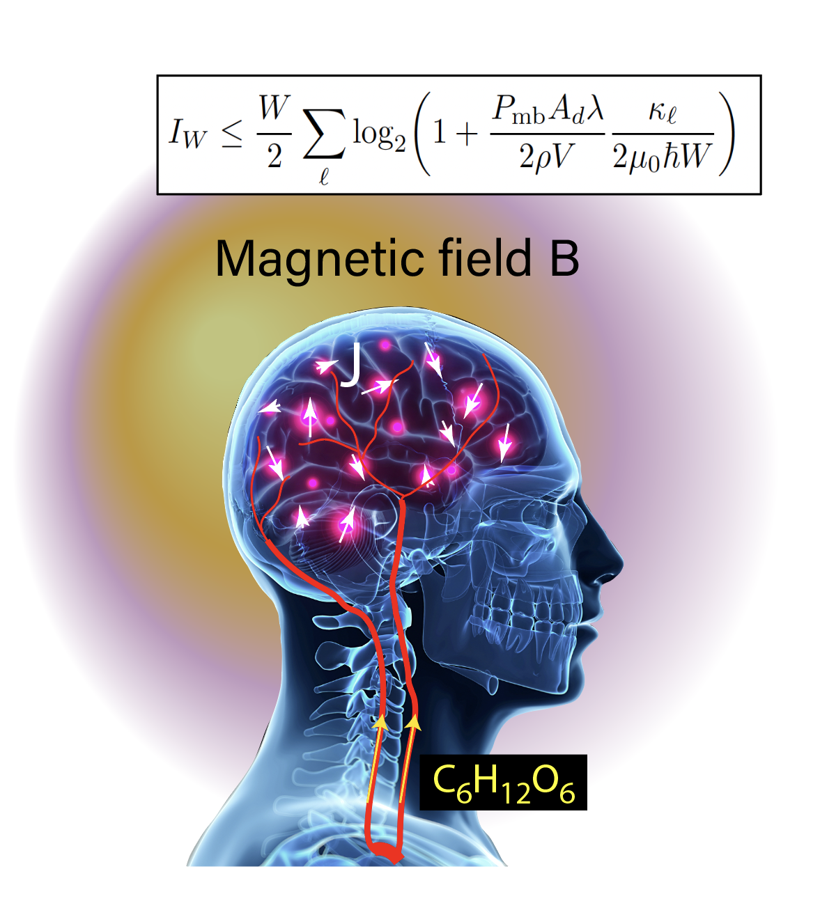
Magnetoencephalography, the noninvasive measurement of magnetic fields produced by brain activity, utilizes quantum sensors like superconducting quantum interference devices or atomic magnetometers. Here we derive a fundamental, technology-independent bound on the information that such measurements can convey. Using the energy resolution limit of magnetic sensing together with the brain's metabolic power, we obtain a universal expression for the maximum information rate, which depends only on geometry, metabolism, and Planck's constant, and the numerical value of which is 2.6 Mbit/s. At the high bandwidth limit we arrive at a bound scaling linearly with the area of the current source boundary. We thus demonstrate a biophysical holographic bound for metabolically powered information conveyed by the magnetic field. For the geometry and metabolic power of the human brain the geometric bound is 6.6 Gbit/s.
Keywords:
magnetoencephalography
; quantum sensing
; information
; holography
As a noninvasive technique imaging brain activity, magnetoencephalography [1,2,3,4,5,6,7,8,9,10,11,12,13,14,15,16] has a history as long as the superconducting quantum interference devices [17,18,19,20,21,22]. Until relatively recently, these have been the only magnetic sensors sensitive enough to detect the feeble magnetic fields generated by the brain’s electric activity. Optical magnetometers [23,24,25] have become a competitive alternative in terms of magnetic sensitivity without requiring any cryogenics, offering a new perspective on the possibilities of magnetoencephalography [26,27,28,29,30,31,32,33,34,35,36,37,38,39,40,41,42,43,44,45,46], and addressing some practical limitations of devices based on superconducting sensors [47].
Both superconducting sensors and optical magnetometers can be operated as absolute field sensors or gradiometers, in single or multiple-sensor whole-head arrangements. The measured signals and the relevant noise sources depend on the particular measurement configuration and physical principles governing each sensor type, respectively. To further develop the applications of quantum sensors to neuroscience [48,49,50,51,52,53,54] and medical diagnosis [55,56,57,58,59,60], it is critical to understand how much information is encoded in these measurements [61], in particular, the upper limit to information that can in principle be retrieved, that is, the information capacity of magnetoencephalography (MEG).
We here obtain a quantum limit to the information capacity of MEG in a general way, irrespective of the particular sensor technology or specific configuration used to acquire MEG signals. To do so, we take advantage of recent developments [62,63] in understanding the fundamental quantum limits to magnetic sensing in a technology-independent way. It was shown [62] and thereafter explained [63], that the energy resolution of numerous sensors of different technologies, given in terms of the variance of the magnetic field estimate, the sensor volume and the measurement time, is bounded below by ℏ.
Using the energy resolution limit (ERL), and connecting the current dipole fluctuations in the brain to the metabolic energy consumed to drive those current sources, we arrive at the quantum limit to the information capacity of MEG expressed in terms of three factors: (i) a geometric (pertaining to the lead-field geometry in the continuous space), (ii) a metabolic (energy consumption of transmembrane ion pumps) and (iii) a quantum (ℏ). In the limit of high bandwidth current sources, we obtain a holographic bound depending on the surface of the source’s boundary, not unlike simliar bounds in black hole thermodynamics. The term “metabolic” goes well beyond semantics and lends itself to an inspiring generalization: biochemical energy → physical observable affected by biochemical energy → quantum sensing of physical observable. This conceptual chain, and the coupling between geometry, metabolism and information could have wide consequences for synthesizing quantum with life.
The information conveyed by MEG measurements is so far quantified by considering a discrete sensor array in specific configurations [61,64,65,66]. We treat the continuum case, where the whole volume outside the head is probed. Consider a finite volume V wherein exist current dipoles described by the density , which generates a magnetic field in the space extending beyond the volume V, and being separated by a minimum distance d from the boundary of V. At position within the magnetic field components are (with )
where
The above, which holds for the case of homogeneous conductivity in the source region, with representing the primary currents [67,68,69,70], can be cast into operator form by introducing the lead-field operator and its adjoint :
Then the field covariance operator is
and has kernel . All spatial correlations of the magnetic field are contained in . Because and is separated from V by a finite distance d, the integral converges. Hence is a compact, positive trace-class operator with eigenvalues (having units ), and .
We now consider random current dipoles with delta-correlated current densities:
where is the variance of the current-dipole density (having units ), and is the same for all three Cartesian components. Importantly, we consider the magnetic field measured with sensors continuously covering the whole region . Even though the underlying current sources are random, the magnetic field exhibits spatial correlations due to the structure of the lead fields (see End Matter). Additionally, there is additive sensor noise contributing to the measured signal . The noise field has covariance
where reflects the magnetic field estimate variance, taken equal for all three Cartesian components ( has units ). Thus, describes a linear map from random currents to random fields. Assuming and are Gaussian, is also Gaussian.
We now evaluate the information conveyed by the measured signal . The source and noise covariance operators are
where and is the identity operator in the Hilbert space of square-integrable vector fields defined in V and , respectively (see End Matter for detailed derivation). Hence the covariance of is
Let be an orthonormal eigenbasis of , , , where the inner product is . The projection of the measured field onto the eigenvectors is
Interpreting the two terms in (11) as “signal” and “noise”, and using independence and zero mean, we have and . Using (5) and (8) we get , and from (9), . Therefore,
The eigenfunctions describe spatial magnetic-field patterns that fluctuate independently. Thus, by Shannon’s formula, the total information obtained from a spatially continuous measurement over is
The eigenvalues quantify how efficiently random currents in V excite independent magnetic-field modes in . The total information I is finite because , a consequence of the compactness of ensured by the finite distance d separating the source volume V from the observation region . The continuous operator thus provides a compact, sensor-independent description of magnetic-field correlations in , determined solely by the lead field and the geometry of the source and measurement domains. Its spectrum defines the fundamental modes through which information about the currents in V is conveyed to , setting an upper bound on the information accessible to any finite array and avoiding convergence issues in discrete limits related to sensor modeling, noise normalization, or weighting.
The utility of the ERL will now become apparent. For a single magnetometer probing one field component over volume v, the energy resolution per unit bandwidth is , and the ERL states that . In the continuum limit , the product remains finite [62], and we identify it with . Thus , where W is the measurement’s bandwidth, and hence the sought after MEG capacity (information in bits/s) reads
For the last step of our derivation, we will connect the variance of the current dipole density, , with the metabolic power, , driving the current dipole sources. We follow the standard approach [71] of considering only intra-dendrite axial currents during excitatory postsynaptic potentials (EPSP) as the dominant contribution to MEG signals. Such currents consist of sodium and calcium ions flowing inward and potassium ions flowing outward, resulting in a net transmembrane current . We approximate the affected dendritic segment with a semi-infinite cylindrical cable of cross section and intracellular resistivity [72]. For a localized injection of at , the solution of the cable equation is an axial current , where is the electrotonic length. This axial current translates into a local current density . Because this current decays exponentially, points separated by more than are effectively uncorrelated. The correlation volume characterizes the region within which current fluctuations remain correlated.
Now, the ohmic dissipation in the volume V is . By identifying this with , we get for the spatial average of , . To connect this coarse-grained quantity to the delta-normalized correlation used in Eq. (6) we multiply by the correlation volume , obtaining . In physical terms, gives the mean squared current density, i.e. the height of its spatial correlation function at zero separation, while represents the width of that correlation. Replacing the finite-range correlation by a delta function should preserve its total integral (height×width), which leads to the expression above. Substituting into (14) yields
This expression is the main result of this work. As stated in the introduction, it is casted in three factors: a geometric factor, , reflecting the geometric coupling of current dipoles into magnetic fields, a metabolic factor, , reflecting the energy driving the current dipoles, and ℏ. The information grows with W. If the current dipole source is band-limited to , increasing the sampling rate W beyond does not increase I. Therefore, the MEG information capacity is given by (14) for .
For an analytically tractable example from which we can readily obtain a numerical estimate, we consider a spherical geometry, i.e. a source region of radius a and observation region consisting of points such that . We use a head radius and . The eigenvalues of , derived in the End Matter, are , with , and they are -degenerate.
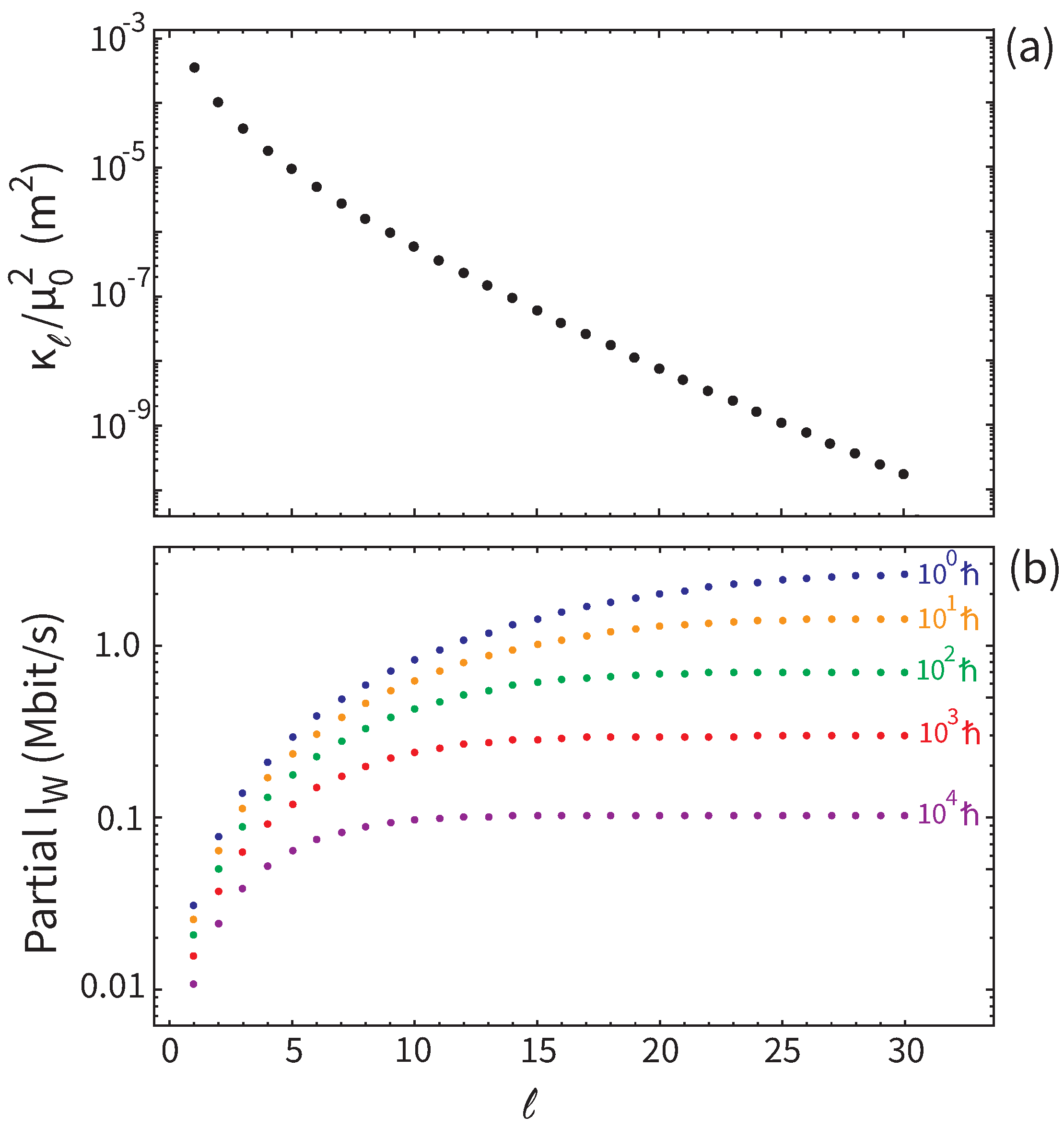
To estimate from the metabolic energy budget [73,74,75,76,77,78,79,80,81,82,83], we first evaluate the total transmembrane current . With being the sodium equilibrium potential, and a sodium driving force of about , the membrane potential is (since ). For potassium it is , so its driving force is about . Assuming equal conductances for Na+ and K+, the currents scale with their driving forces and have opposite directions, giving . Using (inward, with 10% carried by Ca2+) and (inward) [73] yields inward and outward, so the net current is inward. The intra-dendritic resistance for a semi-infinite dendritic cable is . With , , and , this gives . The ohmic power dissipated during an EPSP is then . The corresponding energy, , dissipated over the 1 ms duration of the EPSP [73], is a small fraction of the free energy resulting from the hydrolysis of ATP molecules [79]. Summed over excitatory cortical neurons, each with successful synaptic events per second [82],, the sought-after power is . Overall, for , we find . This numerical estimate does not claim to be any more precise than the numerical values used to derive it. It does show, however, that there is quite some room for acquiring more information with MEG, since state-of-the-art systems report capacities at the level of 400 bits per sample [64], which for the same sampling rate translate to 0.4 Mbit/s. These results are visualized in Figure 1, where we plot the eigenvalues (Figure 1a), and the behavior of (Figure 1b) as a function of the number of eigenvalues included in the sum in the RHS of (15). For the latter plot we use an ERL which ranges from ℏ (fundamental limit) to , so that we cover a broad sensitivity range.
The above can be probed experimentally, since the metabolic power can be influenced e.g. by sleep-wake transitions, or task engagement. Writing the argument of the logarithm in (15) as , we define the sensitivity of information to metabolic drive as . In the biological regime under consideration, it is , thus , where is the total number of modes participating. Thus a scaling of with can in principle reveal both the metabolic law (15) and the number of modes contributing, although within the demanding constraint that the metabolic power can practically vary in the range of only 5% [75,83].
The information bound intertwining geometric, metabolic, and quantum components can be generalized towards several directions. First, one may derive testable scaling laws linking network geometry to achievable information throughput under fixed energetic cost. Second, the metabolic term invites thermodynamic formulations that connect entropy production and energy dissipation to information, along the lines of the Landauer limit [85], this time introducing a quantum sensing aspect. Perhaps more speculatively stated, by coupling these elements, this bound offers a conceptual framework for understanding quantum human-machine interfaces [86]. Alternatively, deviations from this bound may enable discrimination of biological from artificial systems, i.e. a Turing test based on MEG information.
Regarding the latter point, we will here demonstrate a universal bound on information encoded in a magnetic field produced by a metabolically limited “brain”. This bound is holographic, because it depends on the surface of the boundary of the source volume, instead of the volume itself. This is the biophysical analogue of the holographic area law familiar from black-hole thermodynamics [87].
Indeed, let the current source bandwidth, , and accordingly W increase so that in (15) we can make the approximation . Then, setting we get , where
The independence of from the sensor bandwidth reflects a fundamental balance between frequency coverage and quantum noise imposed by the ERL. Shortening the sensor’s measurement time in order to accommodate a fast-changing source leads to increased noise, but at the same time allows faster sampling. In the end the information rate is independent on the sampling rate. Now, for a spherical source it is , derived in the End Matter. For the same parameter values used for the numerical estimate of , we find the numerical value of the holographic bound, .
Interestingly, we notice that for it is . The maximum rate at which magnetic information can be exported from a metabolically active system scales linearly with the energy dissipation rate per system’s volume, and with its geometric boundary. In particular, , reminiscent of the Bekenstein - Hawking entropy that scales as . For human brains the effective operating point is many orders of magnitude below the holographic limit, reflecting the narrow bandwidth of neuronal processes. Artificial systems with broader bandwidths could in principle approach the holographic bound, realizing the full geometric information capacity of the magnetic field produced by localized sources. Brains aside, the current result could also be relevant to astrophysical settings [88].
Concluding, using the technology-independent energy resolution limit to magnetic sensing, a spatially continuous measurement, and the brain’s metabolic power sustaining MEG-active current sources, we have formally derived an upper bound to the information capacity of magnetoencephalography. We have also derived a holographic area law applicable to the high bandwidth limit that can in principle be realized with artificial brains. The concepts elaborated herein can promote connections between neuroscience and quantum technology.
Appendix A. Covariance Operators
In the main text we wrote for the expectation of the random current field outer product,
where is the identity operator in the space of square-integrable vector fields in the volume V. Here we dwell into this formalism. For any two vector fields and defined in V, their outer product is an operator acting on the vector field
where is the inner product in . For a random current density , the ensemble average of this rank-one operator, , is the covariance operator of the random field , having kernel the two-point correlator . This generalizes the concept of a covariance matrix to the continuous case: instead of discrete indices, the kernel depends on two spatial positions and . For delta-correlated current sources it is , thus
Hence indeed it holds . Now, because the magnetic field is a linear functional of the current distribution, , where is the lead-field operator defined in Eq. (3), the outer product of the field can be written directly in terms of that of the current: . Then, the expectation value reads . Using (A1), we find , where is the magnetic field covariance operator introduced in the main text. In other words, the transformation induced by the lead field operator describes the geometric aspect of how uncorrelated current dipoles inside the head lead to spatially correlated magnetic fields outside. The operator , or equivalently its kernel , contains this geometric information. Its eigenfunctions represent statistically independent field modes and its eigenvalues determine the variance, and hence the conveyed information, of each mode.
Appendix B. Trace and Eigenvalues of
The mapping from current sources in V to the magnetic field in is described by the linear operator , with
where is the matrix kernel of , representing the Biot-Savart law
We assume and , with , so that the two regions are disjoint and the subsequent integrals converge.
The composition is a positive, self-adjoint, compact operator on . Its trace is given by the Hilbert–Schmidt norm
where denotes the Frobenius norm .
Because acts as the cross product with , it can be written as the skew-symmetric matrix . Since has singular values , its Frobenius norm satisfies . Thus
To evaluate this double integral, let and . By rotational symmetry,
and therefore
Since
we obtain
Putting everything together gives
This quantity has dimensions , consistent with the Biot–Savart scaling.
Now, is rotationally symmetric in the sense that the Biot–Savart kernel transforms covariantly under rotations. By covariance we mean that for any rotation ,
Define the natural unitary representations of on vector fields in and in V by
Both and are unitary on and , since rotations preserve the Euclidean norm and the integration measure. The covariance property (A9) implies
Hence , so that for all rotations. Thus decomposes into irreducible subspaces with angular momentum ℓ. By Schur’s lemma, acts as a scalar multiple of the identity on each block, .
For any nonzero field , , and taking the inner product gives . Since , it follows that , and therefore .
Now, we consider the exterior harmonic field , with potential in . Its magnitude scales as , therefore . As for the numerator, we start with:
Using the multipole expansion on the boundary ,
and
we find
The surface integral is nonzero only for , so . Finally, the norm of the vector field results in
Dividing by the field norm in gives
Hence the eigenvalues of scale as , with the exact proportionality determined by the trace normalization below. Rotational symmetry then implies -fold degeneracy, and consequently . Setting , and using the identity
we find that
However, the exterior harmonic corresponds to a monopole-like field in . While such a field cannot be produced by real divergence-free currents, the operator acts nontrivially on this mathematical subspace. Thus, to restrict to the physical range of (mapping actual currents to magnetic fields), the spectral sum is taken from upward. Subtracting the monopole contribution gives , so that the final expression is
References
- D. Cohen, Magnetoencephalography: Detection of the brain’s electrical activity with a superconducting magnetometer, Science 175, 664 (1972).
- S. Sato, M. Balish, and R. Muratore, Principles of magnetoencephalography, J. Clin. Neurophysiol. 8, 144 (1991).
- M. Hämäläinen, R. Hari, R. J. Ilmoniemi, J. Knuutila, and O. V. Lounasmaa, Magnetoencephalography - theory, instrumentation, and applications to noninvasive studies of the working human brain, Rev. Mod. Phys. 65, 413 (1993).
- R. C. Knowlton, K. D. Laxer, M. J. Aminoff, T. P. L. Roberts, S. T. C. Wong, and H. A. Rowley, Magnetoencephalography in partial epilepsy: Clinical yield and localization accuracy, Annals Neurol. 42, 622 (1997).
- O. V. Lounasmaa, M. Hämäläinen, R. Hari, and R. Salmelin, Information processing in the human brain: magnetoencephalographic approach, Proc. Natl. Acad. Sci. USA 93, 8809 (1996).
- R. Hari and N. Forss, Magnetoencephalography in the study of human somatosensory cortical processing, Phil. Trans. R. Soc. B 354, 1145 (1999).
- J. Vrba and S. E. Robinson, Signal processing in magnetoencephalography, Methods 25, 249 (2001).
- C. D. Gratta, V. Pizzella, F. Tecchio and G. L. Romani, Magnetoencephalography - a noninvasive brain imaging method with 1 ms time resolution, Rep. Prog. Phys. 64, 1759 (2001).
- G. Nolte, The magnetic lead field theorem in the quasi-static approximation and its use for magnetoencephalography forward calculation in realistic volume conductors, Phys. Med. Biol. 48, 3637 (2003).
- J. W. Wheless, E. Castillo, V. Maggio, H. L. Kim, J. I. Breier, P. G. Simos, and A. C. Papanicolaou, Magnetoencephalography (MEG) and magnetic source imaging (MSI), Neurologist 10, 138 (2004).
- A. S. Fokas, Y. Kurylev, and V. Marinakis, The unique determination of neuronal currents in the brain via magnetoencephalography, Inverse Prob. 20, 1067 (2004).
- A. Hillebrand, K. D. Singh, I. E. Holliday, P. L. Furlong, and G. R. Barnes, A new approach to neuroimaging with magnetoencephalography, Hum. Brain Mapp. 25, 199 (2005).
- D. M. Goldenholz, S. P. Ahlfors, M. S. Hämäläinen, D. Sharon, M. Ishitobi, L. M. Vaina, and S. M. Stufflebeam, Mapping the signal-to-noise-ratios of cortical sources in magnetoencephalography and electroencephalography, Hum. Brain Mapp. 30, 1077 (2009).
- C. J. Stam, Use of magnetoencephalography (MEG) to study functional brain networks in neurodegenerative disorders, J. Neurol. Sci. 289, 128 (2010).
- R. Hari and R. Salmelin, Magnetoencephalography: from SQUIDs to neuroscience, Neuroimage 61, 386 (2012).
- S. Baillet, Magnetoencephalography for brain electrophysiology and imaging, Nature Neurosci. 20, 327 (2017).
- D. Koelle, R. Kleiner, F. Ludwig, E. Dantsker, and J. Clarke, High-transition-temperature superconducting quantum interference devices, Rev. Mod. Phys. 71, 631 (1999).
- J. Vrba and S. E. Robinson, SQUID sensor array configurations for magnetoencephalography applications, Supercond. Sci. and Technol. 15, R51 (2002).
- R. L. Fagaly, Superconducting quantum interference device instruments and applications, Rev. Sci. Instrum. 77, 101101 (2006).
- H.-C. Yang, H.-E. Horng, S. Y. Yang and S.-H. Liao, Advances in biomagnetic research using high-Tc superconducting quantum interference devices, Supercond. Sci. and Technol. 22, 093001 (2009).
- F. Öisjöen, J. F. Schneiderman, G. A. Figueras, M. L. Chukharkin, A. Kalabukhov, A. Hedström, M. Elam, and D. Winkler, High-Tc superconducting quantum interference device recordings of spontaneous brain activity: Towards high-Tc magnetoencephalography, Appl. Phys. Lett. 100, 132601 (2012).
- M. I. Faley, U. Poppe, R. E. Dunin-Borkowski, M. Schiek, F. Boers, H. Chocholacs, J. Dammers, E. Eich, N. J. Shah, A. B. Ermakov, V. Y. Slobodchikov, Y. V. Maslennikov, and V. P. Koshelets, High-Tc DC SQUIDs for magnetoencephalography, IEEE Trans. Appl. Supercond. 23, 1600705 (2013).
- I. K. Kominis, T. W. Kornack, J. C. Allred, and M. V. Romalis, A subfemtotesla multichannel atomic magnetometer, Nature 422, 596 (2003).
- D. Budker and M. V. Romalis, Optical magnetometry, Nature Phys. 3, 227 (2007).
- D. Sheng, S. Li, N. Dural, and M. V. Romalis, Subfemtotesla scalar atomic magnetometry using multipass cells, Phys. Rev. Lett. 110, 160802 (2013).
- H. Xia, A. B.-A. Baranga, D. Hoffman, and M. V. Romalis, Magnetoencephalography with an atomic magnetometer, Appl. Phys. Lett. 89, 211104 (2006).
- C. N. Johnson, P. D. D. Schwindt, and M. Weisend, Multi-sensor magnetoencephalography with atomic magnetometers, Phys. Med. Biol. 58, 6065 (2013).
- K. Kim, S. Begus, H. Xia, S.-K. Lee, V. Jazbinsek, Z. Trontelj, and M. V. Romalis, Multi-channel atomic magnetometer for magnetoencephalography: A configuration study, Neuroimage 89, 143 (2014).
- O. Alem, A. M. Benison, D. S. Barth, J. Kitching, and S. Knappe, Magnetoencephalography of epilepsy with a microfabricated atomic magnetometer, J. Neurosci. 34, 14324 (2014).
- A. P. Colombo, T. R. Carter, A. Borna, Y.-Y. Jau, C. N. Johnson, A. L. Dagel, and P. D. D. Schwindt, Four-channel optically pumped atomic magnetometer for magnetoencephalography, Opt. Express 24, 15403 (2016).
- E. Boto, S. Meyer, V. Shah, O. Alem, S. Knappe, P. Kruger, M. Fromhold, P. Morris, R. Bowtell, G. Barnes, M. Brookes, and M. Lim, A new generation of magnetoencephalography: Room temperature measurements using optically-pumped magnetometers, Neuroimage 149, 404 (2017).
- J. Sheng, S. Wan, Y. Sun, R. Dou, Y. Guo, K. Wei, K. He, J. Qin, and J.-H. Gao, Magnetoencephalography with a Cs-based high-sensitivity compact atomic magnetometer, Rev. Sci. Instr. 88, 094304 (2017).
- A. Borna, T. R. Carter, J. D. Goldberg, A. P. Colombo, Y.-Y. Jau, C. Berry, J. McKay, J. Stephen, M. Weisend, and P. D. D. Schwindt, A 20-channel magnetoencephalography system based on optically pumped magnetometers, Phys. Biol. Med. 62, 8909 (2017).
- E. Boto, N. Holmes, J. Leggett, G. Roberts, V. Shah, S. S. Meyer, L. D. Muñoz, K. J. Mullinger, T. M. Tierney, S. Bestmann, G. R. Barnes, R. Bowtell, and M. J. Brookes, Moving magnetoencephalography towards real-world applications with a wearable system, Nature 555, 657 (2018).
- W. Xiao, C. Sun, L. Shen, Y. Feng, M. Liu, Y. Wu, X. Liu, T. Wu, X. Peng, and H. Guo, A movable unshielded magnetocardiography system, Science Advances 9, eadg1746 (2018).
- T. M. Tierney, N. Holmes, S. Mellor, J. D. López, G. Roberts, R. M. Hill, E. Boto, J. Leggett, V. Shah. M. J. Brookes, R. Bowtell, and G. R. Barnes, Optically pumped magnetometers: From quantum origins to multi-channel magnetoencephalography, Neuroimage 199, 598 (2019).
- J. Iivanainen, R. Zetter, M. Grön, K. Hakkarainen, and L. Parkkonen, On-scalp MEG system utilizing an actively shielded array of optically-pumped magnetometers, Neuroimage 194, 244 (2019).
- D. N. Barry, T. M. Tierney, N. Holmes, E. Boto, G. Roberts, J. Leggett, R. Bowtell, M. J. Brookes, G. R. Barnes, E. A. Maguire, Imaging the human hippocampus with optically-pumped magnetoencephalography, Neuroimage 203, 116192 (2019).
- K. He, S. Wan, J. Sheng, D. Liu, C. Wang, D. Li, L. Qin, S. Luo, J. Qin, and J.-H. Gao, A high-performance compact magnetic shield for optically pumped magnetometer-based magnetoencephalography, Rev. Sci. Instr. 90, 064102 (2019).
- G. Zhang, S. Huang, F. Xu, Z. Hu, and Q. Lin, Multi-channel spin exchange relaxation free magnetometer towards two-dimensional vector magnetoencephalography, Opt. Express 27, 597 (2019).
- E. Labyt, M.-C. Corsi, W. Fourcault, A. P. Laloy, F. Bertrand, and F. Lenouvel, Magnetoencephalography with optically pumped 4He magnetometers at ambient temperature, IEEE Trans. Med. Imaging 38, 90 (2019).
- R. Zhang, W. Xiao, Y. Ding, Y. Feng, X. Peng, L. Shen, C. Sun, T. Wu, Y. Wu, Y. Yang, Z. Zheng, X. Zhang, J. Chen, and H. Guo, Recording brain activities in unshielded Earth’s field with optically pumped atomic magnetometers, Sci. Adv. 6, eaba8792 (2020).
- A. Borna, T. R. Carter, A. P. Colombo, Y.-Y. Jau, J. McKay, M. Weisend, S. Taulu, J. M. Stephen, and P. D. D. Schwindt, Non-Invasive functional-brain-imaging with an OPM-based magnetoencephalography system, PLOS One 15, 1 (2020).
- U. Vivekananda, S. Mellor, T. M. Tierney, N. Holmes, E. Boto, J. Leggett, G. Roberts, R. M. Hill, V. Litvak, M. J. Brookes, R. Bowtell, G. R. Barnes, and M. C. Walker, Optically pumped magnetoencephalography in epilepsy, Annals Clin. Translat. Neurol. 7, 397 (2020).
- M. Rea, E. Boto, N. Holmes, R. Hill, J. Osborne, N. Rhodes, J. Leggett, L. Rier, R. Bowtell, V. Shah, and M. J. Brookes, A 90-channel triaxial magnetoencephalography system using optically pumped magnetometers, Ann. NY Acad. Sci. 1517, 107 (2022).
- O. Feys, P. Corvilain, A. Aeby, C. Sculier, N. Holmes, M. Brookes, S. Goldman, V. Wens, and X. De Tiège, On-scalp optically pumped magnetometers versus cryogenic magnetoencephalography for diagnostic evaluation of epilepsy in school-aged children, Radiology 304, 429 (2022).
- B. Bao, Y. Hua, R. Wang, and D. Li, Quantum-based magnetic field sensors for biosensing, Adv. Quantum Technol. 6, 2200146 (2023).
- R. T. Wakai, A. C. Leuthold, and C. B. Martin, Fetal auditory evoked responses detected by magnetoencephalography, Am. J. Obster. Gynec. 174, 1484 (1996).
- F. J. P. Langheim, A. C. Leuthold, and A. P. Georgopoulos, Synchronous dynamic brain networks revealed by magnetoencephalography, Proc. Natl. Acad. Sci. USA 103, 455 (2006).
- A. A. Ioannides, Magnetoencephalography as a research tool in neuroscience: State of the art, Neuroscientist 12, 524 (2006).
- L. Parkkonen, N. Fujiki, and J. P. Mäkelä, Sources of auditory brainstem responses revisited: Contribution by magnetoencephalography, Hum. Brain Mapp. 30, 1772 (2009).
- R. M. Cichy, A. Khosla, D. Pantazis, and A. Oliva, Dynamics of scene representations in the human brain revealed by magnetoencephalography and deep neural networks, Neuroimage 153, 346 (2017).
- J. Gross, Magnetoencephalography in cognitive neuroscience: A primer, Neuron 104, 189 (2019).
- R. M. Cichy, F. M. Ramirez, and D. Pantazis, Can visual information encoded in cortical columns be decoded from magnetoencephalography data in humans?, Neuroimage 121, 193 (2015).
- D. F. Rose, P. D. Smith, and S. Sato, Magnetoencephalography and epilepsy research, Science 238, 329 (1987).
- R. C. Knowlton and J. Shih, Magnetoencephalography in epilepsy, Epilepsia 45, 61 (2004).
- Magnetoencephalography in neurosurgery, Neurosurgery 59, 493 (2006).
- S. M. Stufflebeam, N. Tanaka, and S. P. Ahlfors, Clinical applications of magnetoencephalography, Hum. Brain Mapp. 30, 1813 (2009).
- I. S. Mohamed, S. A. Gibbs, M. Robert, A. Bouthillier, J.-M. Leroux, and D. K. Nguyen, The utility of magnetoencephalography in the presurgical evaluation of refractory insular epilepsy, Epilepsia 54, 1950 (2013).
- T. W. Wilson, E. Heinrichs-Graham, A. L. Proskovec, and T. J. McDermott, Neuroimaging with magnetoencephalography: A dynamic view of brain pathophysiology, Transl. Res. 175, 17 (2016).
- P. K. Kemppainen and R. J. Ilmoniemi, Channel capacity of multichannel magnetometers, in Advances in biomagnetism, edited by (S. J. Williamson et al., Plenum Press, New York, 1989).
- M. W. Mitchell and S. P. Alvarez, Colloquium: Quantum limits to the energy resolution of magnetic field sensors, Rev. Mod. Phys. 92, 021001 (2020).
- I. K. Kominis, Quantum thermodynamic derivation of the energy resolution limit in magnetometry, Phys. Rev. Lett. 133, 263201 (2024).
- J. F. Schneiderman, Information content with low- vs. high-Tc SQUID arrays in MEG recordings: The case for high-Tc SQUID-based MEG, J. Neurosci. Meth. 222, 42 (2014).
- J. Iivanainen, M. Stenroos, and L. Parkkonen, Measuring MEG closer to the brain: Performance of on-scalp sensor arrays, Neuroimage, 147, 542 (2017).
- E. Skidchenko, N. Yavich, A. Butorina, M. Ostras, P. Vetoshko, M. Malovichko, and N. Koshev, Yttrium-Iron Garnet magnetometer in MEG: Advance towards multi-channel arrays, Sensors 23, 4256 (2023).
- D. B. Geselowitz, On bioelectric potentials in an inhomogeneous conductor, Biophysical J. 7, 1 (1967).
- D. B. Geselowitz, On the Magnetic Field Generated Outside an Inhomogeneous Volume Conductor by Internal Current Sources, IEEE Trans. Magn. 6, 346 (1970).
- J. Sarvas, Basic mathematical and electromagnetic concepts of the biomagnetic inverse problem, Phys. Med. Biol. 32, 11 (1987).
- J. C. Mosher, R. M. Leahy, and P. S. Lewis, EEG and MEG: Forward Solutions for Inverse Methods, IEEE Trans. Biomed. Eng. 46, 245 (1999).
- R. Plonsey, The nature of sources of bioelectric and biomagnetic fields, Biophysical J. 39, 309 (1982).
- D. Johnston and S. M.-S. Wu, Foundations of cellular neurophysiology (MIT Press, Cambridge 1995).
- D. Attwell and S. B. Laughlin, An Energy budget for signaling in the grey matter of the brain, J. Cereb. Blood Flow Metab. 21, 1133 (2001).
- P. Lennie, The cost of cortical computation, Current Biol. 13, 493 (2003).
- M. E. Raichle, Two views of brain function, Trends Cogn. Sci. 14, 180 (2010).
- C. Howarth, C. M. Peppiatt-Wildman, and D. Attwell, The energy use associated with neural computation in the cerebellum, J. Cereb. Blood Flow Metab. 30, 403 (2010).
- C. Howarth, P. Gleeson, and D. Attwell, Updated energy budgets for neural computation in the neocortex and cerebellum, J. Cereb. Blood Flow Metab. 32, 1222 (2012).
- J. J. Harris and D. Attwell, The energy of CNS white matter, J. Neurosci. 32, 356 (2012).
- R. J. Clarke, M. Catauro, H. H. Rasmussen, and H. Apell, Quantitative calculation of the role of the Na+,K+-ATPase in thermogenesis, Biochim. Biophys. Acta 1827, 1205 (2013).
- E. Engl and D. Attwell, Non-signaling energy use in the brain, J. Physiol. 16, 3417 (2015).
- E. Engl, R. Jolivet, C. N. Hall, and D. Attwell, Non-signalling energy use in the developing rat brain, J. Cereb. Blood Flow Metab. 37, 951 (2017).
- Y. Yu, P. Herman, D. L. Rothman, D. Agarwal, and F. Hyder, Evaluating the gray and white matter energy budgets of human brain function, J. Cereb. Blood Flow Metab. 38, 1339 (2017).
- S. D. Jamadar, A. Behler, H. Deery, and M. Breakspear, The metabolic costs of cognition,’Trends Cogn. Sci. 29, 541 (2025).
- R. van Uitert, D. Weinstein, and C. Johnson, Volume Currents in Forward and Inverse Magnetoencephalographic Simulations Using Realistic Head Models, Annals Biomed. Eng. 31, 21 (2003).
- S. Deffner and S. Campbell, Quantum thermodynamics (Morgan & Claypool Publishers, 2019).
- M. Zhu, T. He, and C. Lee, Technologies toward next generation human machine interfaces: From machine learning enhanced tactile sensing to neuromorphic sensory systems, Appl. Phys. Rev. 7, 031305 (2020).
- R. M. Wald, The thermodynamics of black holes, Living Rev. in Rel. 4, 6 (2001).
- X. Guo, P. Wang, and H. Yang, Membrane paradigm and holographic DC conductivity for nonlinear electrodynamics, Phys. Rev. D 98, 026021 (2018).
Figure 1.
(a) The first 30 eigenvalues of normalized by , for and . (b) Partial information obtained from (15) by letting the sum over ℓ extend from 1 to , and generalizing the ERL to be in the range from ℏ (the fundamental limit) up to . It is seen that the more sensitive the sensor, the more spatial modes of are required to saturate .
Disclaimer/Publisher’s Note: The statements, opinions and data contained in all publications are solely those of the individual author(s) and contributor(s) and not of MDPI and/or the editor(s). MDPI and/or the editor(s) disclaim responsibility for any injury to people or property resulting from any ideas, methods, instructions or products referred to in the content. |
© 2025 by the authors. Licensee MDPI, Basel, Switzerland. This article is an open access article distributed under the terms and conditions of the Creative Commons Attribution (CC BY) license (http://creativecommons.org/licenses/by/4.0/).
Copyright: This open access article is published under a Creative Commons CC BY 4.0 license, which permit the free download, distribution, and reuse, provided that the author and preprint are cited in any reuse.


