
Submitted:
05 November 2025
Posted:
06 November 2025
You are already at the latest version
Abstract
Aviation permanent magnet synchronous motors (PMSMs) are particularly susceptible to demagnetization faults due to the thermal sensitivity of permanent magnet materials, compounded by high-altitude conditions where reduced air density significantly limits cooling. In addition, the pursuit of high power density and compact structure in aviation design intensifies local thermal stress, while stringent reliability requirements mean even minor degradation can threaten operational safety. This paper investigates the operating characteristics of aviation PMSMs under demagnetization faults and proposes an effective diagnostic approach. A coupled electromagnetic–thermal finite element model is established to evaluate rated and no-load performance and calculate losses under rated conditions, and its validity for the motor body is confirmed using the RT-LAB semi-physical simulation platform. Subsequently, altitude-dependent ambient air parameters are incorporated to analyze the thermal–magnetic field distribution, highlighting the influence of high-altitude operation. Based on the thermal results, a fault dataset is constructed by selecting typical local demagnetization cases and classifying global faults into levels according to temperature criteria, with features extracted in both time and frequency domains. Finally, an intelligent diagnostic method integrating a deep belief network (DBN) and an extreme learning machine (ELM) is developed. Comparative results demonstrate superior accuracy and robustness over conventional methods, advancing demagnetization fault diagnosis for aviation PMSMs.
Keywords:
PMSM
; coupled multi-physics permanent magnet demagnetization
; fault diagnosis
; deep learning
1. Introduction
Electric aircraft have attracted significant research attention due to their potential for reduced noise, improved environmental sustainability, and reduced reliance on fossil fuels [1,2]. For lift and cruise applications, high power density is essential [3]. Permanent magnet synchronous motors (PMSMs) are widely applied in electric aircraft because of their simple structure, excellent controllability, high energy density, and reliability. However, at high altitudes, low atmospheric pressure, reduced air density, and low ambient temperature significantly weaken convective cooling. Combined with their inherently high power density, aviation PMSMs are prone to heat accumulation. Rising motor temperature can cause demagnetization of the permanent magnets, leading to torque reduction, eccentric rotation, or even catastrophic motor failure [4]. Therefore, investigating and diagnosing demagnetization faults under coupled multi-physics conditions is crucial for aviation PMSMs.
Scholars have conducted extensive research on the precise diagnosis of demagnetization faults in permanent magnet synchronous motors to enhance their operational lifespan and reliability. A key focus of this research is achieving accurate time-frequency signal characterization for the early detection of these faults. Reference [5] employs a wavelet transform-based motor current signature analysis technique to analyze current signals under transient operating conditions. Using finite element analysis techniques, Reference [6] created demagnetization fault models of permanent magnet motors at various levels. The target parameter was the stator current signal, and wavelet transform was used to analyse the current spectrum properties. A diagnostic of local demagnetization faults in the motor was finished, based on the characteristic frequencies produced by demagnetization faults in the stator current. Reference [7] proposed a diagnostic method that combines wavelet packet and sample entropy. Through mathematical derivation and analysis, the method determines the fault characteristic frequency by judging the frequency components of the stator current and the reconstruction nodes of wavelet packet transformation, which was then experimentally verified. The results showed that the 5th and 7th harmonic components were significantly affected by demagnetization faults and could be used as targets for detection and diagnosis. The above references used time-frequency methods to diagnose demagnetization faults through various time-frequency extraction or transformation methods. However, the time-frequency methods have certain limitations. Overall demagnetization faults do not produce an asymmetric magnetic field, and the spectral changes of motor signals under overall demagnetization faults are not obvious. Therefore, using only time-frequency methods cannot effectively distinguish between overall demagnetization faults and local demagnetization faults. Reference [8] proposed an online fault diagnosis method for permanent magnet synchronous motors (PMSMs) targeting typical rotor faults (demagnetization and eccentricity), based on spatiotemporal characteristics of stator tooth flux. By establishing a mathematical model of stator tooth flux under fault conditions and employing a multi-search coil detection device, the method achieves effective fault feature extraction and type identification. Reference [9], considering saturation characteristics, stator slot structure, and degree of faults, diagnosed faults of surface-mounted permanent magnet synchronous motors by analyzing the motor output torque and using finite element analysis to simulate and verify the faults. Reference [10] detected the harmonic components of induced electromotive force caused by shaft oscillations under demagnetization faults and verified it through an improved finite element method. These methods diagnose faults by detecting the torque or induced electromotive force and current. Fault detection based on zero sequence components of induced electromotive force is affected by changes in speed, while fault diagnosis based on torque fluctuations relies on precise sensors and is susceptible to vibration interference. Reference [11] proposed a physics-based method for identifying the fault indicator for the demagnetization of permanent magnet synchronous motors with no fractional harmonics during its operation and found that the 8th harmonic component in stator current waveform is a good indication for the demagnetization of PMSM. Reference [12] locates demagnetization faults by installing three toroidal-yoke-type search coils in stator slots to construct fault location signals. Two fault indicators extracted from these signals under various demagnetization fault conditions are input into a knowledge graph for fault positioning, while demonstrating its applicability across motors with different structural designs. Reference [13] diagnosed demagnetization faults based on measuring magnetic flux of stator tooth, determining the position and scope of demagnetization based on signal transformation of the measured magnetic flux by sensors, which can effectively distinguish between overall demagnetization and local demagnetization faults. These methods observe or estimate the operating state of the motor based on parameters such as motor phase voltage, current, magnetic flux, and speed. Diagnosis of demagnetization faults is based on the trend of these parameters. But these methods heavily depend on motor parameters, and factors such as motor geometry, winding layout, observer performance. Thus, these factors can all have a certain impact on the method.
To address these challenges, this paper develops a finite element method (FEM)-based framework to analyze the electromagnetic characteristics of aviation PMSMs under no-load, rated, and multiple demagnetization fault conditions. Motor losses under rated operating conditions are calculated, and a coupled magneto–thermal multi-physics model is established considering ambient air at flight altitude. Based on the thermal response, several levels of overall demagnetization are classified, and representative local demagnetization cases are selected. Characteristic data under different fault conditions are extracted and preprocessed. To enhance diagnostic performance, an enhanced fireworks algorithm (EnFWA) is introduced to optimize a hybrid model consisting of a deep belief network (DBN) and an extreme learning machine (ELM), enabling accurate diagnosis and classification of demagnetization faults.
2. Finite Element Modeling and Magneto–Thermal Analysis of Aviation PMSMs
2.1. Electromagnetic Modeling of Aviation PMSMs
High power density is required for interior PMSMs used in aviation applications. Permanent magnet (PM) is one of the core components of PMSMs. PM material determines the electromagnetic performance of the motor. However, due to their high temperature sensitivity, PM materials should be chosen with high remanence and coercive force, and with the highest possible temperature tolerance At the same time, due to the scarcity of rare earth materials, cost considerations are also essential. To sum up, NdFeB material is selected in this paper and the B-H curve of the material at normal temperature is shown in Figure 1.
On the account of magnetic resistance of air gap, most of the energy is stored in the air gap. A relatively small air-gap width is conducive to improving the magnetic flux density and reducing leakage loss. In addition, it reduces the overall motor size and increases the energy density. The trapezoidal slot has a larger internal and a smaller opening area, which facilitates the arrangement of windings and keeps the slot fill factor within a suitable range. Double-layer windings have two layers of windings in each slot with insulation between each layer. The double-layer winding can be designed to suppress high harmonics. According to Equation (1), the number of slots per pole per phase is determined to be 3.
Z is the number of stator slots. p is pole pairs. m is the number of phase. q is the number of slots per pole per phase.
2.2. Analysis of Electromagnetic Characteristics
As the no-load back electromotive force (BEF) of the motor is an important parameter, the no-load BEF E0 can be calculated with Equation (2).

f is electrical frequency. K is winding coefficient. N is number of turns. Φ is average magnetic flux through winding. No-load BEF and its amplitude of odd harmonics during a single electrical period are extracted and shown in Figure 3. The three-phase no-load BEF has a approximate sinusoidal waveform and each odd harmonic component is low relative to the fundamental component. The amplitude of odd harmonics of no-load BEF is summarized in Table 2 and the U phase is taken as an example to give the percentage of odd harmonics proportion as shown in Table 3.
It can be seen from Table 3 that the percentage of each odd harmonic of the no-load back-EMF is mostly lower than 3%. From the above analysis, it can be concluded that the motor runs under the rated operating condition.
Figure 4 shows the spatial magnetic flux density distribution of the air gap under no-load conditions. The magnetic flux density distribution of the motor at each pole is reasonable and approximately sinusoidal in circumferential space. The magnetic flux density of the air gap fluctuates because of the PM arrangement and the cogging effect of the stator. The rated output torque of the motor is shown in Figure 5. The torque pulsates to a certain extent because of the existence of cogging torque.
PMSMs will produce various kinds of losses under rated conditions where the electrical frequency is higher. Figure 6 shows the loss curve of the steel material. Because of the high frequency of aviation power supply, the rotor adopts a laminated structure to reduce eddy current loss. In addition, under high electrical frequency, the loss increases significantly, and methods for reducing the loss should be considered. Moreover, the cooling and heat dissipation capacity of the motor should be improved accordingly.
Loss of PMSMs mainly includes iron loss, winding eddy loss, permanent magnet hysteresis loss and mechanical loss. Accurate calculation of loss is the basis of coupled multi-physics modeling. The most widely used calculation method for iron loss is Bertotti’s model, which divides iron core loss into three parts: hysteresis loss, core loss and excess loss[14]. The expression is as follow:
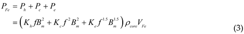
PFe is iron loss. Ph is hysteresis loss. Pc is core loss. Pe is excess loss. f is core magnetization frequency. Bm is amplitude of magnetic density. Kh is hysteresis loss coefficient. Kc is core loss coefficient. Ke is excess loss coefficient. ρcore is density of the core. VFe is core magnetization volume.
In the calculation of steady thermal model, the initial heat source of the model is defined by the heat generation rate. The calculation formula of the heat generation rate q is shown as equation(4):
Q is total heat. V is volume. Therefore, the heat generation rate of each part of the motor is obtained. Except the coil which is calculated in root mean square, other parts are calculated in average.

Table 4.
loss and heat generation rate.
| Parts | Loss(W) | Heat generation rate(W·m-3) |
|---|---|---|
| Stator | 746.3 | 95856.45 |
| Rotor | 235.98 | 44060.07 |
| PM | 22.68 | 375000 |
| Coil | 27.78 | 1392481.2 |
To further validate the accuracy of the finite element electromagnetic model, a semi-physical simulation was conducted on the RT-LAB platform. The OP5700 real-time simulator, which integrates a multi-core target computer, a reconfigurable FPGA, and modular I/O conditioning boards, is particularly suitable for verifying the complex operational requirements of aviation PMSMs. It supports high-speed data exchange through fiber-optic channels and up to 256 I/O lines, enabling flexible interfacing with external systems.
In this study, the OP5700 was configured to reproduce the rated operating conditions of the motor, allowing real-time execution of the PMSM model and providing dynamic responses consistent with practical operation. This setup ensures that finite element analysis (FEA) results can be cross-verified in a real-time environment, establishing a complementary validation framework that bridges the gap between offline simulations and actual operating conditions. Figure 7 shows the OP5700 simulator used in this study.
In this process, the key electromagnetic parameters obtained from the finite element model—such as resistance, inductance, flux linkage, and torque characteristics—were imported into RT-LAB. These parameters ensured that the semi-physical simulation model preserved the electromagnetic behavior of the PMSM predicted by FEA. A comparison of the output torque between the RT-LAB simulation and the finite element analysis is presented in Figure 8, confirming the consistency of both approaches and validating the reliability of the electromagnetic model.
The finite element model directly simulates the steady-state operation results of the motor, whereas the semi-physical simulation model is a dynamic model that requires a certain duration to reach a stable state. Its output fluctuates less, and the output torque tends to stabilize after 4000 points, reflecting good control performance. The output torque finally stabilizes at about 34.3 N·m, with an error of approximately 0.58% compared with the mean output torque of the finite element model.
2.3. Thermal Modeling of Aviation PMSMs
The distribution of loss is symmetrical due to the symmetry of the motor’s geometric structure. Although the internal structure of the motor is complex, most of the losses are concentrated in the windings, stator, and rotor. Therefore, in order to balance computational accuracy and modeling effort, the internal structure of the motor can be simplified to some extent.
The motor windings are designed in double layers and are evenly distributed in the stator slots. Each winding consists of multiple turns of wire, with each turn coated in insulating rubber to prevent short-circuit faults. However, an excessive number of turns makes the thermal model overly complex while contributing little to the improvement of analysis accuracy. Hence, each winding can be regarded as an independent thermal structure with an insulating coating on its surface. The double-layer winding structure consists of two identical layers, which can be equivalently modeled as two parallel conductors. The equivalent structure is illustrated in Figure 9.
In order to reduce eddy current loss, the stator and rotor adopt a laminated structure, with each layer coated in insulation to ensure electrical isolation and mitigate the eddy current effect. Since the thermal study is conducted under steady-state conditions and assumes uniform heat dissipation across all components, the stator and rotor are treated as equivalent whole structures in the thermal analysis, and their dimensions remain unchanged after equivalence [15]. Figure 10 illustrates the equivalent structure.
Aviation PMSMs operate under diverse conditions as aircraft undergo taxiing, climbing, cruising, descending, and landing throughout the flight cycle. These phases are accompanied by variations in altitude, which cause significant changes in the external environment. With increasing altitude, the air density and pressure decrease markedly, the ambient temperature drops, and the convective cooling capacity of the surrounding airflow is substantially weakened. Among these flight phases, the cruise stage occupies the largest proportion of the total duration and is therefore selected as the representative operating background in this study. At present, the cruising altitude of all-electric aircraft is typically within the range of 1000 m to 5000 m. To account for the most demanding cooling condition and ensure sufficient thermal dissipation margin, a cruising altitude of 5000 m is adopted in the analysis.
The changes in the dynamic viscosity and thermal conductivity of air with altitude can be determined using Sutherland’s equation [16].
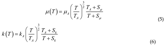
Sμ and Sk are constants; TA, μA and kA are the Kelvin temperature, dynamic viscosity and thermal conductivity at a temperature of 0℃, respectively. Therefore, the physical parameters of the air at an altitude of 5000m can be calculated, the physical parameters of air at 0 m and 5000 m altitude are presented in Table 5.
It is necessary to simplify the thermal model to balance computational efficiency and accuracy. The following assumptions are made:
(1) The fluid inside the motor is considered incompressible.
(2) Gravitational and buoyancy effects of the fluid are neglected.
(3) The fluid flow is assumed to be laminar.
After applying these assumptions, an equivalent thermal model of the motor is established. At an altitude of 5,000 m, the external environment markedly alters the motor’s heat dissipation conditions. Due to reduced air density and lower pressure, the efficiency of forced convection cooling is significantly weakened, limiting the ability of airflow to remove heat from the motor surface. As a result, heat accumulation in the windings, stator, and permanent magnets becomes more pronounced, and the overall thermal distribution shifts toward higher equilibrium temperatures. Although the axial temperature difference remains relatively small because of uniform airflow, the absolute temperature rise increases the risk of magnet demagnetization and insulation degradation. The computational domain is then defined, where the forward wall of the z-axis is set as the velocity inlet and the reverse wall as the pressure outlet, while the other four walls are treated as adiabatic. Figure 11 illustrates the complete configuration, with the four adiabatic walls hidden for clarity.
These assumptions and boundary conditions not only simplify the model while maintaining accuracy, but also provide a consistent basis for coupling electromagnetic loss distribution with the thermal field, enabling an integrated magneto-thermal analysis of the aviation PMSM.
2.4. Process and result analysis of magneto-thermal coupling
In aviation PMSMs, the electromagnetic and thermal fields are strongly coupled, and the high-altitude environment further aggravates thermal challenges due to reduced air density and weakened convection. Magneto-thermal coupling analysis is therefore essential. To balance computational cost and accuracy, this paper adopts a one-way coupling approach, where electromagnetic losses obtained from finite element analysis are introduced as heat sources in the thermal model. This method provides reliable results while maintaining computational efficiency. On this basis, the main steps of magneto-thermal coupling analysis are as follows:
(1) Firstly, the magnetic analysis model and the thermal analysis model of the aviation PMSM are established respectively and the loss of each part of the motor is obtained from the magnetic field analysis.
(2) Initialization of thermal parameters is settled mainly including equivalent modeling, the initial heat generation rate and thermal conductivity calculating.
(3) The computational domain and boundary conditions are defined. Specifically, inlet and outlet conditions are set along the motor’s z-axis to simulate forced convection, while the remaining walls are treated as adiabatic. The initial temperature distribution and fluid parameters are assigned in accordance with high-altitude ambient conditions, consistent with the assumptions described in the previous section.
(4) All conditions settled, the magneto-thermal coupling model will be run normally. According to the temperature curve of each part, whether the whole motor reaches a stable state will be determined. If the temperature is not stable, the number of simulation steps needs to be increased until the temperature is stable.
The flow chart is shown in Figure 12:
The simulation results are shown in Figure 13. The permanent magnet starts at an initial temperature of 20 ℃ and stabilizes at approximately 114 ℃ after several iterations. Other motor components also reach steady-state conditions following transient fluctuations, where notable temperature variations occur before rated operation is established. The laminated structure effectively mitigates heat generation in the rotor, stator, and permanent magnets; however, for high-power motors, additional cooling strategies remain essential to prevent insulation degradation and potential short-circuit faults. Figure 14 depicts the temperature distribution of the motor. Due to forced convection, the front region maintains relatively lower temperatures, while the axial temperature gradually increases toward the rear. Nonetheless, the temperature difference between the two ends is small, indicating that demagnetization tends to occur globally rather than locally. This thermally induced demagnetization modifies the electromagnetic performance of the motor, leading to distortions in current, back-EMF, and torque. These variations provide measurable indicators that form the basis for subsequent fault analysis and diagnosis.
3. Analysis and Diagnosis of Demagnetization Fault
3.1. Modeling of demagnetization fault
According to the results of magneto–thermal coupling analysis, the motor is divided into six groups using a 20 ℃ temperature gradient, ranging from the initial 20 ℃ to 120 ℃, which is slightly above the steady-state temperature. Each temperature level corresponds to a specific degree of demagnetization. The classification is further justified by the thermal characteristics of NdFeB permanent magnets: when the operating temperature exceeds approximately 120 ℃, the magnets exhibit a significant reduction in flux density, while temperatures above 150℃ may lead to irreversible demagnetization. Thus, the adopted grouping not only reflects the numerical results of thermal simulation but also aligns with the physical demagnetization thresholds of the magnet material. Table 6 presents the detailed relationships.
PMSMs may suffer local demagnetization faults due to permanent magnet aging, mechanical collisions, or other factors. A local demagnetization fault causes torque reduction and fluctuation, which may induce rotor eccentricity faults and significantly degrade the motor’s output performance. Although both overall and local demagnetization faults lead to reduced output torque, their causes are different, making it necessary to distinguish between them. In this paper, two types of local demagnetization faults are investigated: 20% and 40% demagnetization of a single magnetic pole. The air-gap magnetic flux density curve is extracted, and when local demagnetization occurs, its spatial distribution becomes distorted, as shown in Figure 15. The fault parameters are summarized in Table 7.
3.2. Feature analysis of demagnetization fault
The remanence and coercivity of a permanent magnet decrease with the increase of temperature. The demagnetization rate Dem of a permanent magnet can be shown in equation(7).
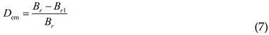
Br is the initial remanence and Br1 is the remanence under the current demagnetization. Most of the magnetic energy is stored in the air gap for the large magnetic reluctance. Therefore, the magnetic density of the air gap becomes an important target to measure the magnetic performance of the motor. Fundamental magnetic flux per pole is shown as equation(8):
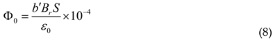
b' is the per unit value of the magnetic flux density under the current working condition of the permanent magnet. S is the cross-sectional area of each pole. ε0 is the no-load magnetic leakage coefficient. No-load air gap magnetic density B0 is shown in equation(9).
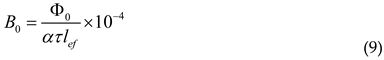
α is the polar arc coefficient. τ is the pole pitch. lef is the length of the core. As shown in formula and , it can be seen that the fundamental flux of each pole decreases due to the reduction of remanence when demagnetization faults occur, which resulting in the decrease of the air gap magnetic density and the output performance of the motor.
The input electric power P1 can be expressed as:

PCu is the copper loss. Electromagnetic power Pe can be expressed as:

PFe is the iron loss. PΩ is the mechanical loss. P2 is the output mechanical power on the shaft. Pe can also be expressed as:
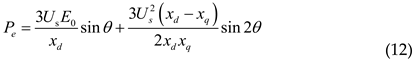
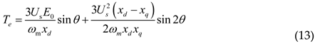
Us is the RMS value of the phase voltage. xq and xd are the reactance of quadrature and direct axis respectively. ωm is the mechanical angular velocity. θ is the power angle. For the interior PMSM, the electromagnetic torque Te of the motor is divided into basic torque and reluctance torque because of the inequality of quadrature and direct axis reactance. The expression of Te is as follows:
When the motor operates under no-load conditions, the air-gap magnetic field mainly consists of permanent magnet flux. The amplitude and waveform of the air-gap magnetic flux density are directly determined by the remanence of the permanent magnet. When the motor operates under load, the air-gap magnetic field consists of the permanent magnet field and the field generated by the windings. Due to the winding field, the impact of demagnetization faults on the air-gap magnetic field is relatively weakened. Figure 16 illustrates the no-load and load air-gap magnetic flux density waveforms under six levels of overall demagnetization faults.
When temperature of the motor rises to 120℃, that is, the overall demagnetization fault Ⅵ occurs, the air gap magnetic density of both conditions decreases to a certain extent and the reduction is more obvious under no-load operation. Figure 17 can be obtained by intercepting a positive half period of no-load and load air gap magnetic density and taking its average value. It can be seen from Figure 17 that under no-load and load conditions, the mean value of magnetic density decreases with the increase of demagnetization degree. Under the influence of winding magnetic field, the average magnetic density of air gap is larger.
The frequency components of the airgap magnetic extracted from six kinds of overall demagnetization faults are shown in Table 8. With the increase of demagnetization degree, the fundamental amplitude of the air gap magnetic density decreases significantly and other odd harmonics also decrease to varying degrees except the ninth harmonic.
The three-phase voltage shows a decreasing trend as temperature rises, as shown in Figure 18. After extracting the single-phase voltage for FFT analysis, the amplitude of the fundamental frequency component decreases significantly, while the amplitudes of other frequency components, such as the 5th, 13th, and 15th harmonics, exhibit significant variations. At lower temperatures, the voltage does not decrease markedly and exhibits a nonlinear variation with increasing temperature.
Overall demagnetization faults lead to a decrease and fluctuation in output torque. The effect is approximately linear within a relatively low temperature range and exhibits an accelerated decline as temperature increases, as shown in Figure 19.
Local demagnetization faults destroy the symmetry of the air-gap magnetic field, causing the magnetic density to generate several specific frequency harmonics. These harmonics can be expressed as:
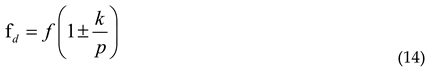
fd is the characteristic frequency of local demagnetization faults. f is the fundamental frequency. p is the number of pole-pairs. k is a positive integer.
Taking the magnetic density of the stator as an example, the characteristic frequency components of local demagnetization faults are analyzed. According to the equation, several components are generated around the fundamental frequency. Figure 20 illustrates the details, and specific data are presented in Table 9. For different values of k, the characteristic components in equation (14) are 133.33, 266.67, 533.33, 666.67, 800, 933.33, etc. The calculated results agree with the tabulated data.
The characteristic frequency of local demagnetization faults can be used to distinguish overall demagnetization faults from local demagnetization faults. This characteristic frequency introduces harmonic components into the three-phase voltage. The time and frequency characteristics of the single-phase voltage are shown in Figure 21. Local demagnetization faults lead to characteristic components in the three-phase voltage. Therefore, local demagnetization faults can be diagnosed by extracting the stator voltage frequency and analyzing the amplitudes of specific frequency components.
On account of the asymmetry in the magnetic density distribution under local demagnetization faults, it is deduced that the motor’s voltage and torque will be affected, thereby producing harmonics. Local demagnetization faults weaken the magnetic field generated by the permanent magnets and cause a reduction in output torque, potentially leading to a mismatch between the motor output torque and the load torque. Such asymmetry may also result in eccentric faults when the magnetic pull on the rotor becomes unbalanced. The output torque under demagnetization faults is shown in Figure 22.
As can be seen from Figure 22, within the range of demagnetization studied in this paper—specifically 20% and 40% demagnetization of a magnetic pole—local demagnetization faults cause greater torque loss than overall demagnetization faults. A rapid decline in torque intensifies the imbalance on the motor’s output shaft, resulting in deceleration, strong current pulsations, and mechanical vibrations, all of which threaten the structural safety of the motor.
The preceding analyses identified the characteristic features of demagnetization faults and clarified their impact on motor behavior. To translate these insights into an effective fault diagnosis, a systematic framework is required to extract representative features, ensure robustness against interference, and achieve reliable classification. The following section develops such a diagnostic framework and evaluates its performance.
4. Diagnostic Framework and Performance Evaluation
4.1. Diagnostic Model and Optimization
Traditional time-frequency methods for PMSM fault diagnosis are often limited by their sensitivity to motor geometry and operating conditions, making feature extraction unreliable in complex environments. Deep learning–based approaches, by contrast, can directly learn representative fault characteristics from signal data without relying on the specific structure or operating principles of the machine. To exploit this advantage, this study adopts a hybrid diagnostic framework that integrates a Deep Belief Network (DBN) with an Extreme Learning Machine (ELM).
The DBN, composed of multiple Restricted Boltzmann Machines (RBMs), extracts hierarchical features from input signals through unsupervised pretraining and refines them via supervised fine-tuning. The extracted features are then classified by the ELM, which offers fast training speed and strong generalization ability. By combining the DBN’s feature representation capability with the ELM’s classification efficiency, the proposed framework achieves higher diagnostic accuracy and robustness in identifying PMSM demagnetization faults. The structure of the RBM is shown in Figure 23. During the training stage, the DBN extracts characteristic information from the input signal, while in the fine-tuning stage, the parameters are adjusted according to the error.
As a classifier, ELM has a typical three-layer structure consisted of the input layer, the hidden layer and the output layer. The output of ELM oi is shown in equation (15):
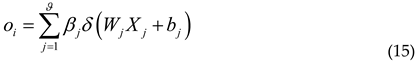
W is the ELM hidden layer weight matrix. b is the ELM hidden layer bias vector. ϑ is the number of ELM hidden layer nodes. i is the number of label layers. β is the weight matrix between the hidden layer and the label layer. X is the output value of the upper-layer. In this paper, ELM, as a label classifier of fault diagnosis model, is placed in the last layer of the model.
Since the diagnostic performance of the DBN–ELM model is highly sensitive to hyperparameter selection, this study introduces an Enhanced Fireworks Algorithm (EnFWA) for optimization. Compared with the traditional Fireworks Algorithm, EnFWA incorporates a dynamic adjustment factor q and a dynamic radius factor μr, expressed as in (16) and (17):
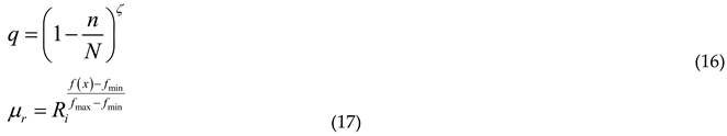
n is the current number of iterations. N is the maximum number of iterations. ζ is the adjustment coefficient. f(x) is the fitness function of the algorithm. fmin and fmax is the minimum and maximum value of the fitness function. Ri is the search radius under the current fitness value.
Additionally, EnFWA adopts a roulette-based selection strategy, which dynamically adjusts the search radius as fitness updates, accelerating convergence and reducing the risk of local optima. This optimization ensures that the DBN–ELM model achieves an efficient and robust structure for fault diagnosis.
4.2. Process of fault diagnosis and result analysis
Before constructing the diagnostic framework, it is necessary to clarify the rationale for feature extraction. Demagnetization faults in PMSMs manifest primarily as distortions in magnetic flux density, torque fluctuations, and variations in induced voltage. Torque provides a direct reflection of the motor’s electromechanical performance, while the three-phase induced voltage contains abundant fault-related information in both the time and frequency domains. By applying FFT, the frequency components of induced voltage can be decomposed to identify harmonics that are particularly sensitive to demagnetization. Specifically, global demagnetization is often associated with an increase in the third harmonic due to flux asymmetry, whereas local demagnetization typically produces sideband components near the fundamental frequency. These harmonic variations provide discriminative features that strengthen the separability of different fault modes.
Based on this rationale, the diagnostic dataset is constructed from both time-domain and frequency-domain indicators. The sampled signals include the motor’s output torque and the three-phase induced voltage. FFT analysis is applied to the induced voltage, and each phase is decomposed into 1025 frequency components. The sampling frequency is set to 20 kHz, with a duration of 0.75 s, yielding four time-domain indexes and three frequency-domain indexes under each fault mode. For accuracy and generality, 30 sets of data are recorded per fault, of which 25 are used for model training to determine optimal parameters and 5 for testing. The final data and labels are summarized in Table 10.
Data from the eight demagnetization faults form a 240×63075 matrix. During the actual sampling process of motor, disturbances such as mechanical and electromagnetic interference are inevitably present. To simulate real-world conditions, Gaussian white noise is introduced to corrupt the sampled data. Standardization and normalization processing are carried out. Figure 24 shows the effect of white noise. Data in the figure are frequency components of U phase voltage.
The fault diagnosis model adopts the combination of DBN-ELM and the diagnosis flow chart is shown in Figure 25. The details are as follows:
(1) Demagnetization fault data are obtained using the multi-physical coupling analysis method.
(2) Noise is introduced to simulate real-world operating conditions. The data are then standardized, normalized, and divided into training and testing sets, with labels assigned accordingly.
(3) An optimization algorithm is employed to tune the hyperparameters of the model, thereby obtaining the optimal structure.
(4) The training data are input into the model for learning, and the testing data are subsequently used to perform fault diagnosis.
The results of a single diagnosis are shown in Figure 26. The accuracy of the training set reached 91.5%, while that of the test set reached 87.5%. More error points occur in the overall demagnetization faults because the differences among the six fault types are relatively small. The distribution of the other error points is irregular, which may be attributed to the presence of white noise.
In order to further verify the accuracy of the diagnostic model, three benchmark models are selected for comparison.
(1) SDAE+SVM: stacked denoised autoencoder (SDAE) is used to extract features from the original data and reduce the overall dimension of the data. support vector machine (SVM) is used to classify the data and corresponding fault labels. The hidden layer network structure is [30,75,150]. The sparse coefficient is 0.01. The penalty term has a weight of 2.
(2) CNN+Softmax: convolutional neural networks (CNN) are used for feature extraction and the last layer of the network is classified by softmax classifier. The model has 5 convolutional layers. The size of the convolution kernel in the first layer is 64´1, and the remaining 4 layers are 3´1. The number of neurons in the fully connected layer is 100 and the activation function is Relu function. The softmax layer has eight outputs corresponding to eight faults.
(3) LSTM: model adopts a two-layer LSTM (Long Short Term Memory) structure. The number of neurons in each layer is 20. The Dropout parameter is set to 0.4 and the bottom layer adopts a fully connected layer to classify output.
Table 11.
Comparison.
| Training accuracy (%) | Test accuracy (%) | Duration(s) | |
|---|---|---|---|
| DBN-ELM | 92 | 85 | 9.2 |
| SDAE+SVM | 89 | 82 | 38.7 |
| CNN+softmax | 100 | 87.5 | 21.4 |
| LSTM+Dense | 87.5 | 85.7 | 54.1 |
The model consists of SDAE and SVM have poor accuracy and long training time. The accuracy of the training set of the diagnostic model CNN+Softmax is better, but the accuracy of the test set is decreased, which means the diagnosis is unstable. The low data dimension may lead to overfitting of the model. The results of the LSTM diagnostic model are stable and the accuracy of the training set and the test set have hardly differences but both of them are relative low. Compared with the processing of time series data, the performance of LSTM in the processing of classification diagnosis is dissatisfactory. In summary, the diagnostic model proposed in this paper has a higher degree of accuracy and rapidity compared with other models.
5. Conclusions
In this paper, a multi-physics coupling approach was employed to establish and analyze demagnetization fault models of an interior PMSM. The results indicate that under rated operating conditions, the air-gap magnetic density exhibits distortions, with a clear increase in the third harmonic component. The motor experiences considerable losses under aircraft power excitation, and even with forced convection cooling, a non-negligible temperature rise remains. The thermal field tends toward uniformity in the core, while the permanent magnets are susceptible to global demagnetization. Consequently, both the output torque and induced voltage—particularly torque—show an accelerated decline. For local demagnetization, the fault characteristics vary with fault location and are typically manifested as increases in several frequency components near the fundamental frequency, though the magnitude of these increases differs among cases. Furthermore, the proposed DBN–ELM diagnostic framework demonstrates strong capability in extracting fault-relevant features and distinguishing among different demagnetization conditions, thereby improving diagnostic efficiency. Compared with conventional methods, the integration of electromagnetic–thermal coupling with intelligent diagnosis provides a more comprehensive understanding of fault mechanisms. Overall, the study offers not only detailed insights into the electromagnetic–thermal interactions of aviation PMSMs but also a validated diagnostic strategy that may contribute to enhancing operational reliability in aviation applications.
Author Contributions
Zhangang Yang: Conceptualization, Writing-review and editing, Methodology, Formal analysis, Supervision. Xiaozhong Zhang: Conceptualization, Writing-original draft, Formal analysis, Validation, Writing-review and editing, Data curation.
Acknowledgments
This research is supported by the Tianjin Key Laboratory of Aeronautical Power Distribution System (PD2024-KF03).
Conflicts of Interest
The authors declare no conflicts of interest.
References
- Sarlioglu, B.; Morris, C.T. More Electric Aircraft: Review, Challenges, and Opportunities for Commercial Transport Aircraft. IEEE Transactions on Transportation Electrification 2015, 1, 54–64. [Google Scholar] [CrossRef]
- Gohardani, A.S.; Doulgeris, G.; Singh, R. Challenges of future aircraft propulsion: A review of distributed propulsion technology and its potential application for the all electric commercial aircraft. Progress in Aerospace Sciences 2011, 47, 369–391. [Google Scholar] [CrossRef]
- Schefer, H.; Fauth, L.; Kopp, T.H.; Mallwitz, R.; Friebe, J.; Kurrat, M. Discussion on Electric Power Supply Systems for All Electric Aircraft. IEEE Access 2020, 8, 84188–84216. [Google Scholar] [CrossRef]
- Guopei, W.; Yinquan, Y.; Wenbing, T. Review of research on fault diagnosis of permanent magnet synchronous motor. Chinese Journal of Engineering Design 2021, 28, 548–558. [Google Scholar] [CrossRef]
- Singh, M.; Dubey, G.; Gupta, D.; Siddiqui, K.M.; Chauhan, B.K. "Modelling. Simulation and Early Diagnosis of PMSM Demagnetization Fault," 2022 1st International Conference on Sustainable Technology for Power and Energy Systems (STPES), SRINAGAR, India, 2022, pp. 1–6. [CrossRef]
- Ruiz, J.R.R.; Rosero, J.A.; Espinosa, A.G.; et al. Detection of demagnetization faults in permanent-magnet synchronous motors under nonstationary conditions. IEEE Transactions on Magnetics 2009, 45, 2961–2969. [Google Scholar] [CrossRef]
- Zhiyan, Z.; Hongzhong, M.; Cunxiang, Y.; et al. Demagnetization fault diagnosis in permanent magnet synchronous motor combination wavelet packet with sample entropy. Electric Machines and Control 2015, 19, 26–32. [Google Scholar] [CrossRef]
- Zeng, C.; Huang, S.; Lei, J.; Wan, Z.; Yang, Y. Online Rotor Fault Diagnosis of Permanent Magnet Synchronous Motors Based on Stator Tooth Flux. IEEE Transactions on Industry Applications 2021, 57, 2366–2377. [Google Scholar] [CrossRef]
- Ebrahimi, B.M.; Faiz, J. Demagnetization fault diagnosis in surface mounted permanent magnet synchronous motors. IEEE Transactions on Magnetics 2013, 49, 1185–1192. [Google Scholar] [CrossRef]
- Urresty, J.C.; Atashkhooei, R.; Riba, J.R.; et al. Shaft trajectory analysis in a partially demagnetized permanent-magnet synchronous motor. IEEE Transactions on Industrial Electronics 2013, 60, 3454–3461. [Google Scholar] [CrossRef]
- Ko, Y.; Lee, Y.; Oh, J.; Park, J.; Chang, H.; Kim, N. Current signature identification and analysis for demagnetization fault diagnosis of permanent magnet synchronous motors. Mechanical Systems and Signal Processing 2024, 214, 111377. [Google Scholar] [CrossRef]
- Gao, C.; Gao, B.; Xu, X.; Si, J.; Hu, Y. Automatic Demagnetization Fault Location of Direct-Drive Permanent Magnet Synchronous Motor Using Knowledge Graph. IEEE Transactions on Instrumentation and Measurement 2024, 73, 3502312. [Google Scholar] [CrossRef]
- Chong, Z. Research on Fault Diagnosis of Permanent Magnet synchronous Motor Based on Stator Tooth Flux[D]. Chongqing: Chongqing university, 2019. [CrossRef]
- Bertotti, G. General properties of power losses in soft ferromagnetic materials. IEEE Transactions on Magnetics 1988, 24, 621–630. [Google Scholar] [CrossRef]
- Qihao, F. Analysis of Loss and Temperature Field of High Speed Maglev Permanent Magnet Motor[D]. Wuhan: Wuhan University of Technology, 2021. [CrossRef]
- Cao, K. A study of fundamental heat transfer behavior at near-space altitudes [C], Year.
- Hinton, G.E.; Salakhutdinov, R.R. Reducing the dimensionality of data with neural networks. Science 2006, 313, 504–507. [Google Scholar] [CrossRef] [PubMed]
- Huang, G.-B.; Zhu, Q.-Y.; Siew, C.-K. Extreme learning machine: Theory and applications. Neurocomputing 2006, 70, 489–501. [Google Scholar] [CrossRef]
Figure 1.
Magnetization curve.
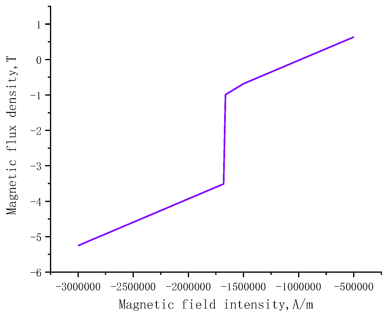
Figure 2.
Finite element model and mesh.
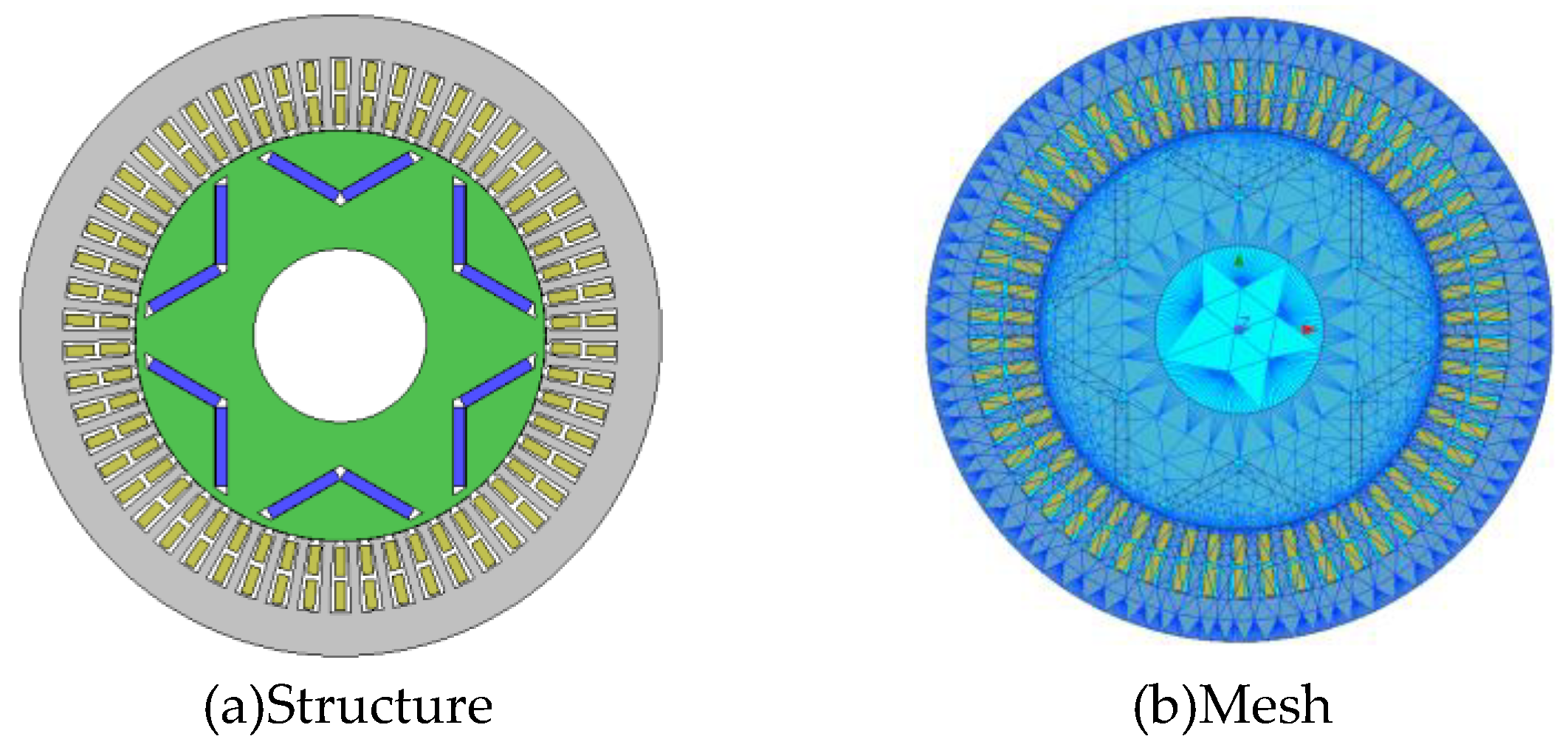
Figure 3.
Analysis of back electromotive force.
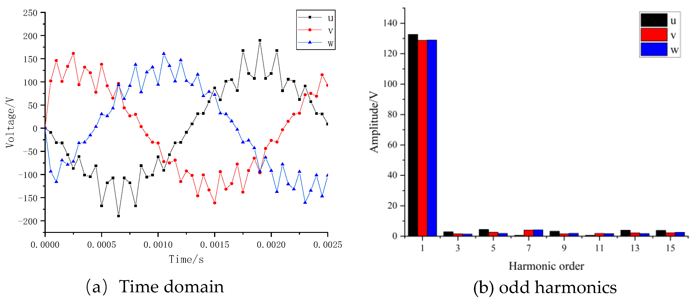
Figure 4.
Spatial magnetic density distribution.
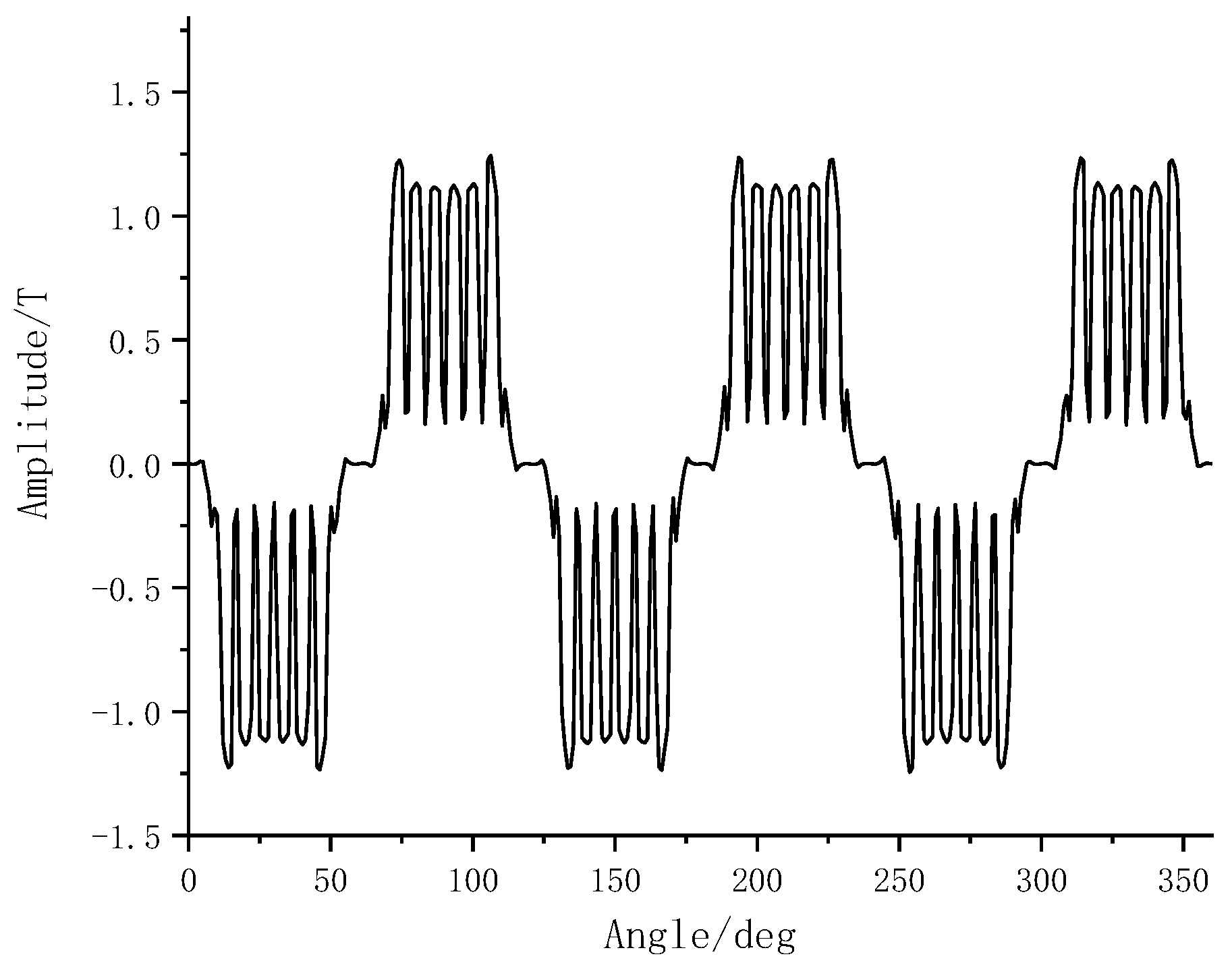
Figure 5.
Output torque.
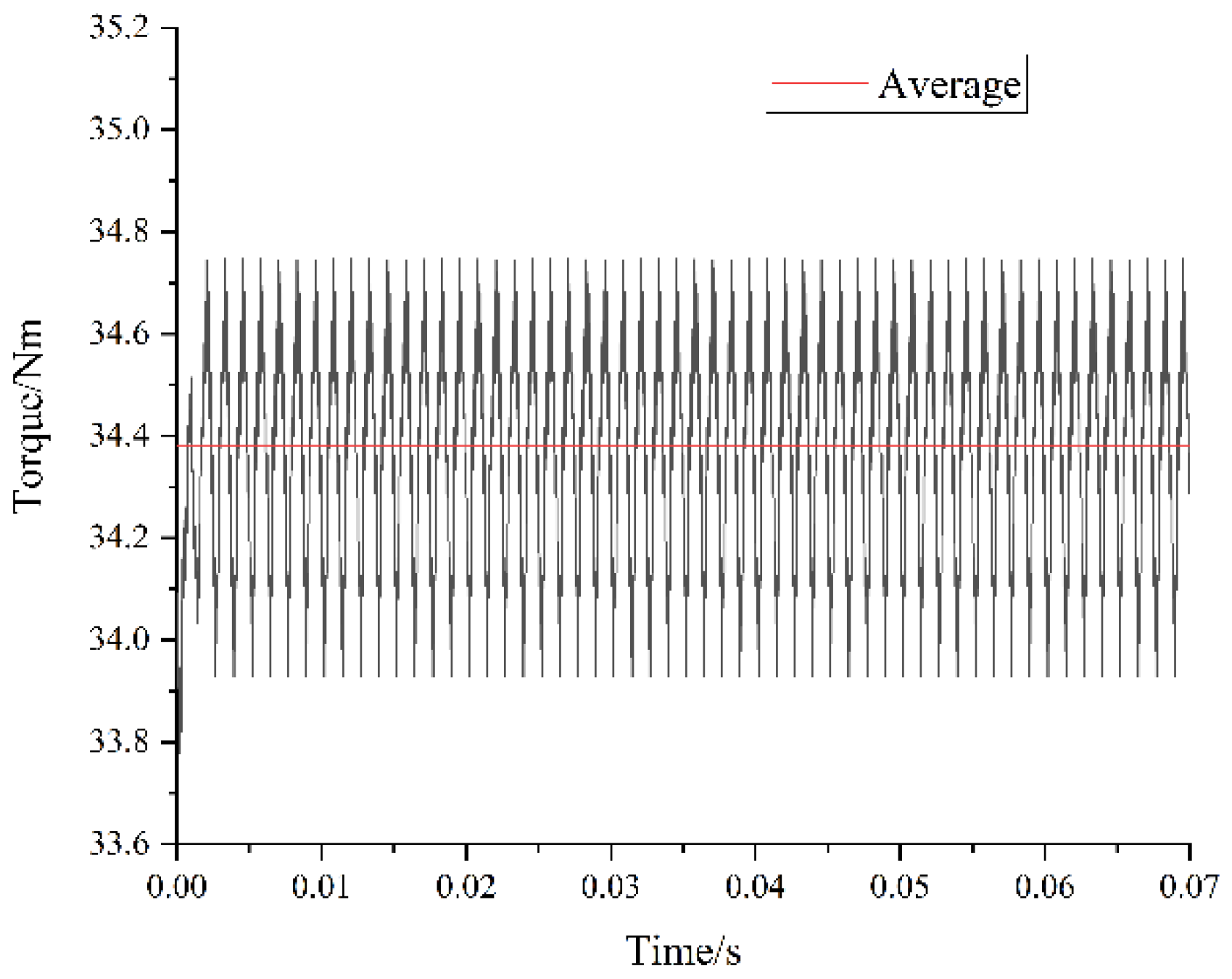
Figure 6.
Loss characteristic.
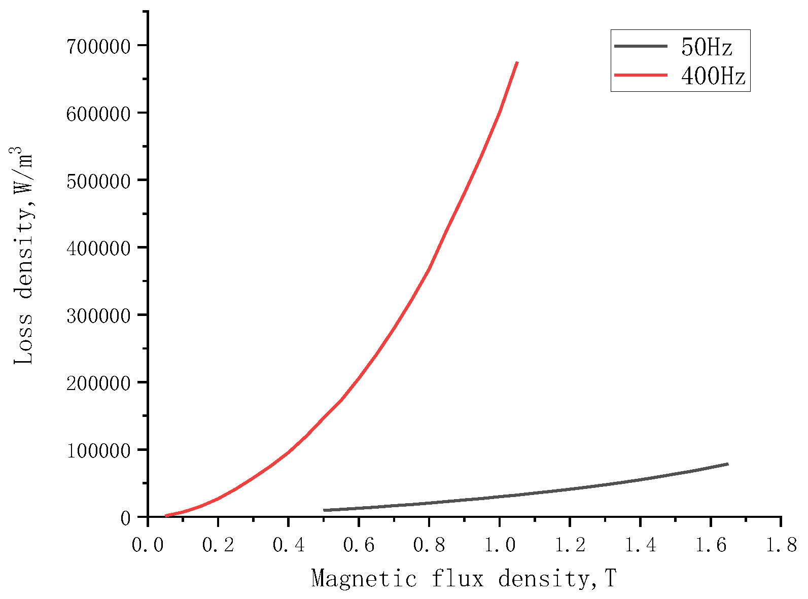
Figure 7.
OP5700.
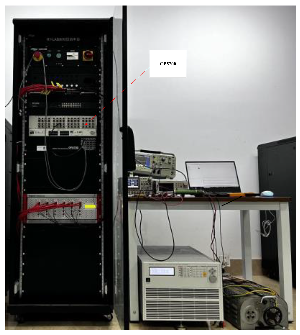
Figure 8.
Torque comparison.
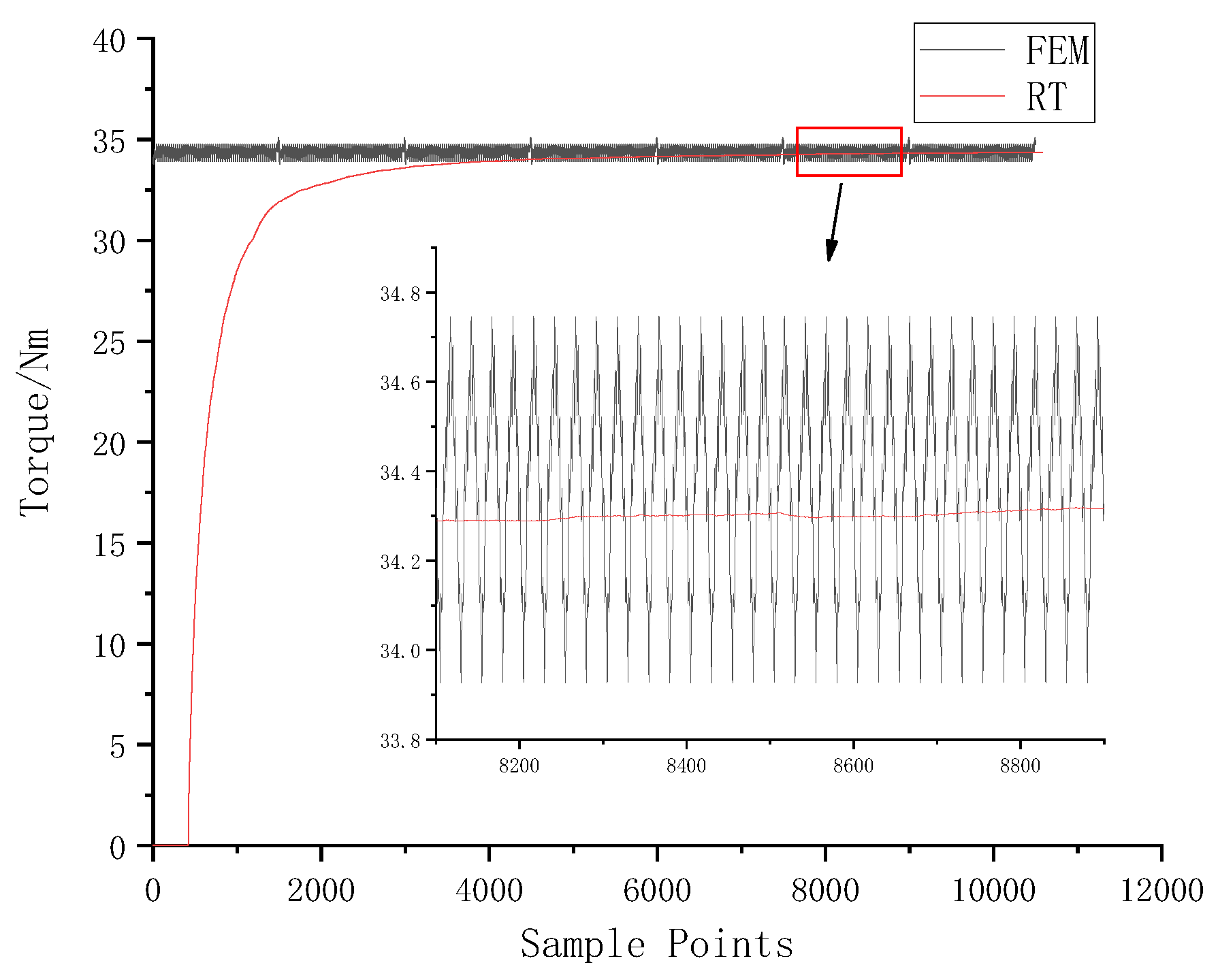
Figure 9.
Equivalent model of winding.
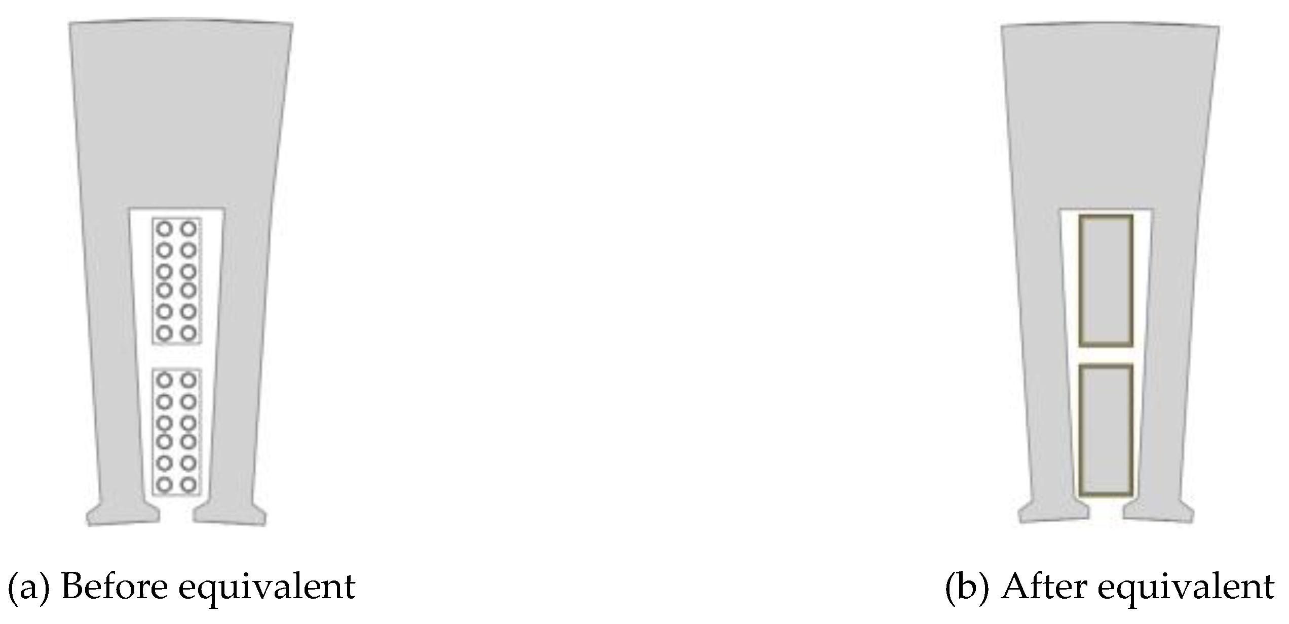
Figure 10.
Equivalent model of stator.
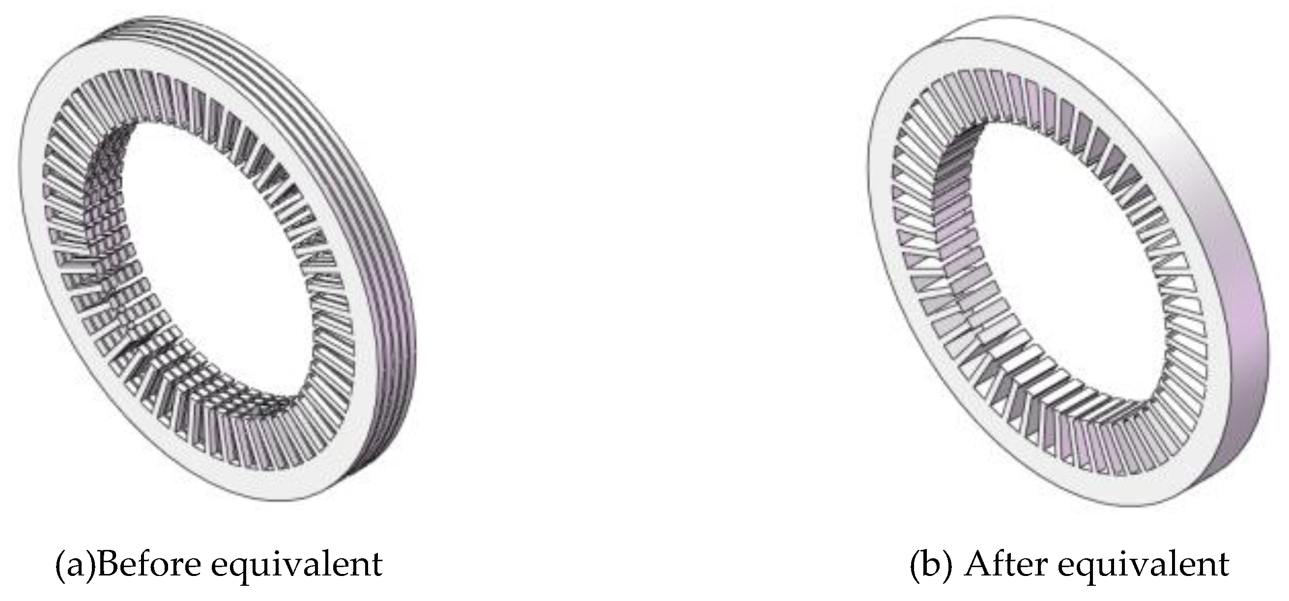
Figure 11.
Thermal simulation model.
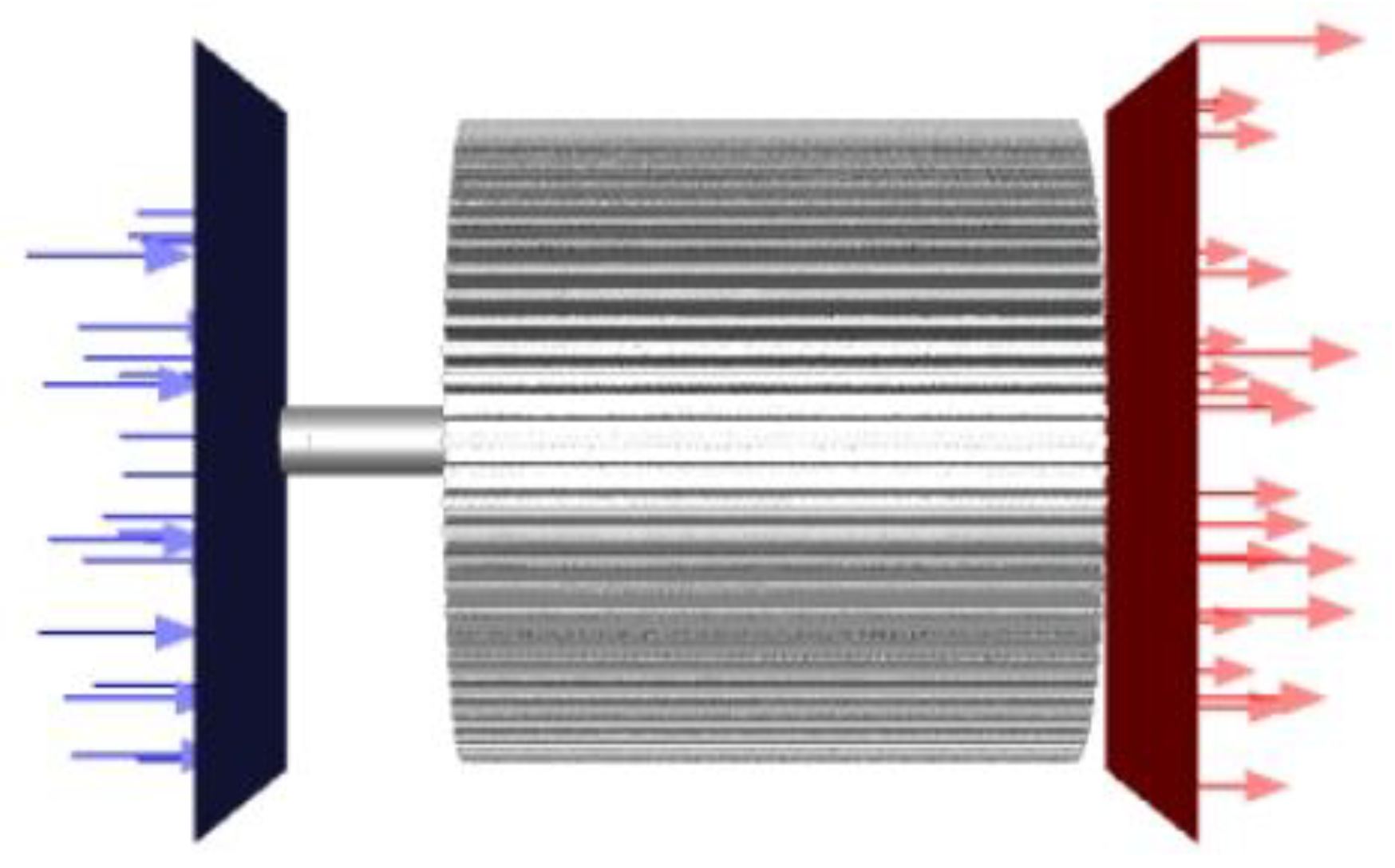
Figure 12.
Flow chart of the magneto-thermal coupling model.
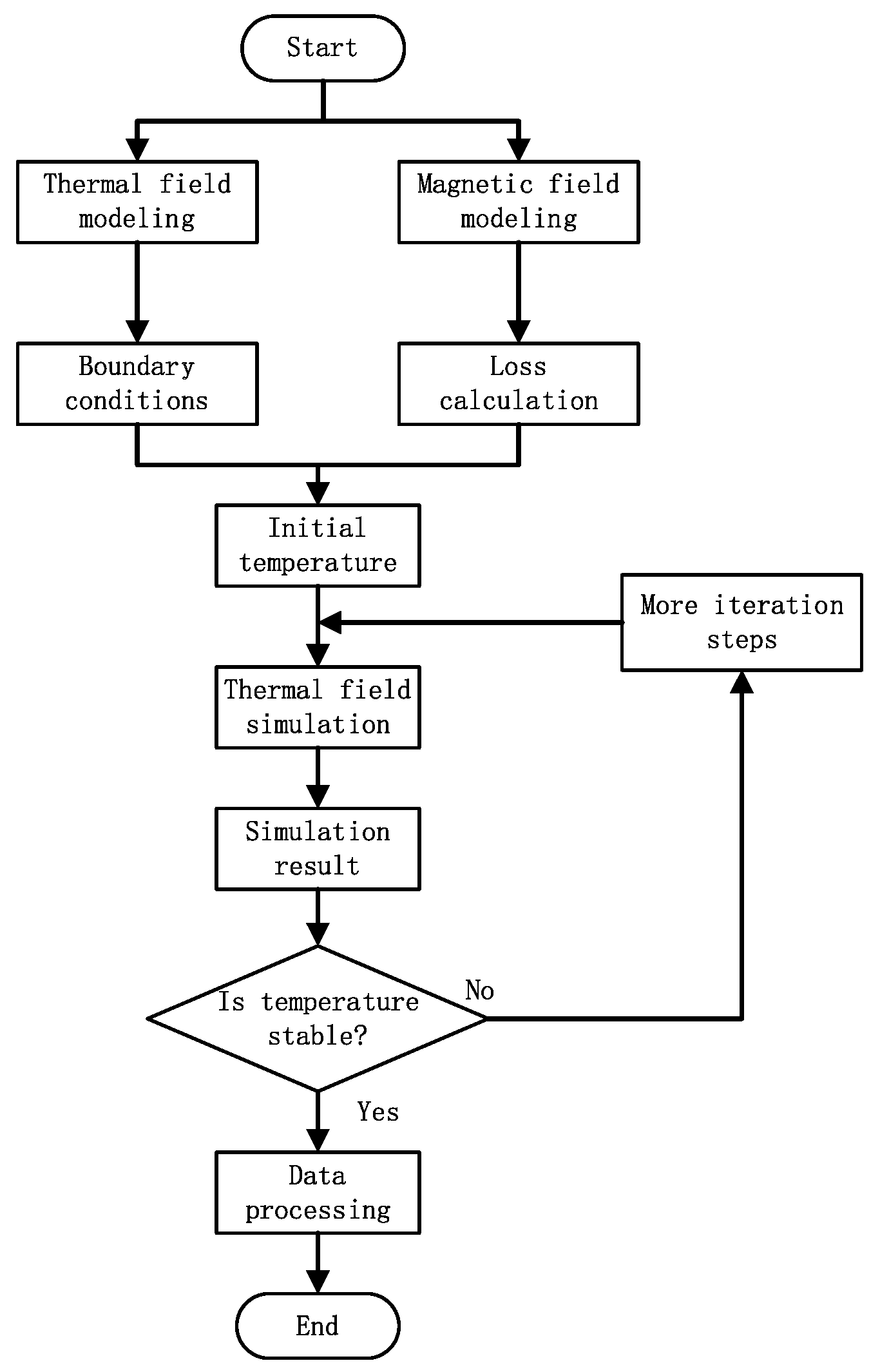
Figure 13.
Temperature curve.
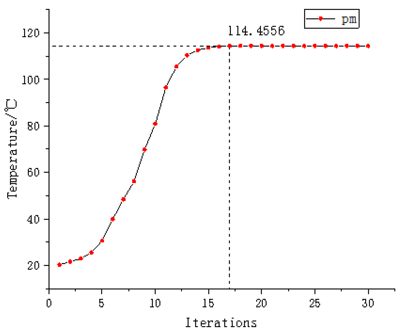
Figure 14.
Temperature distribution contour.
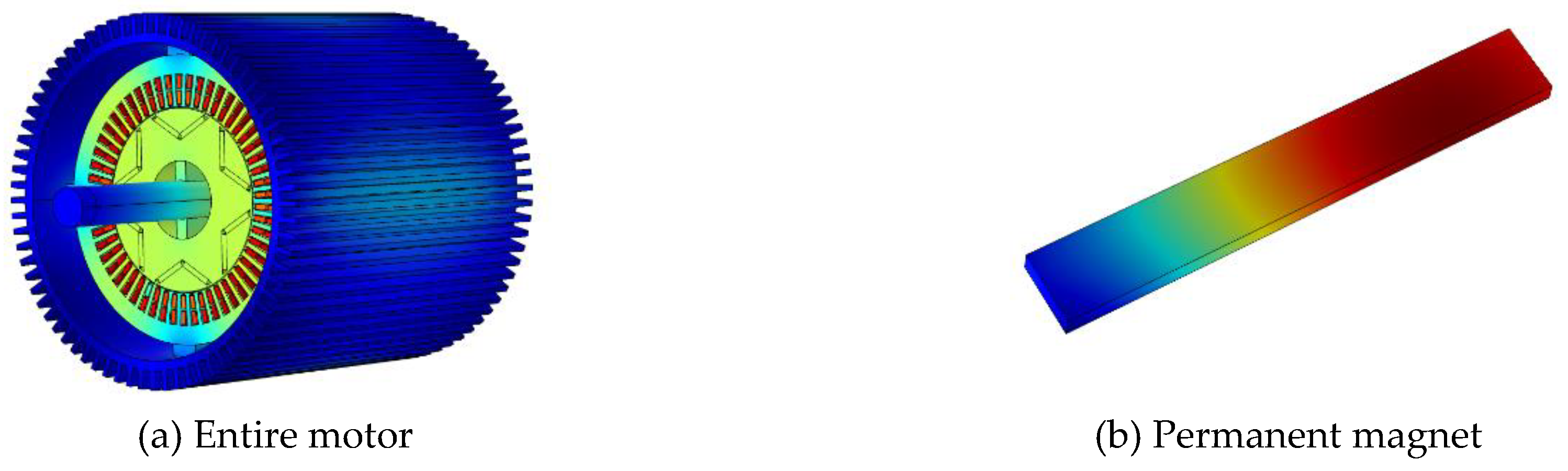
Figure 15.
spatial distribution of air gap magnetic density.
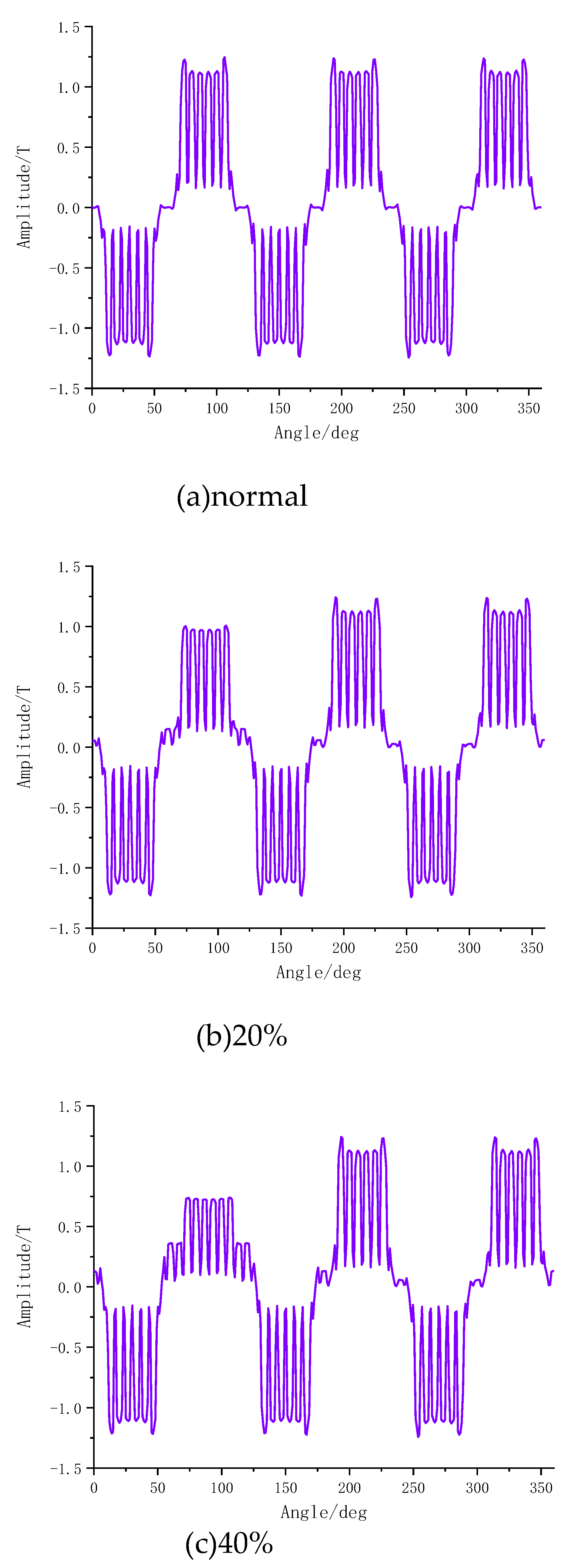
Figure 16.
Air gap magnetic density waveform.
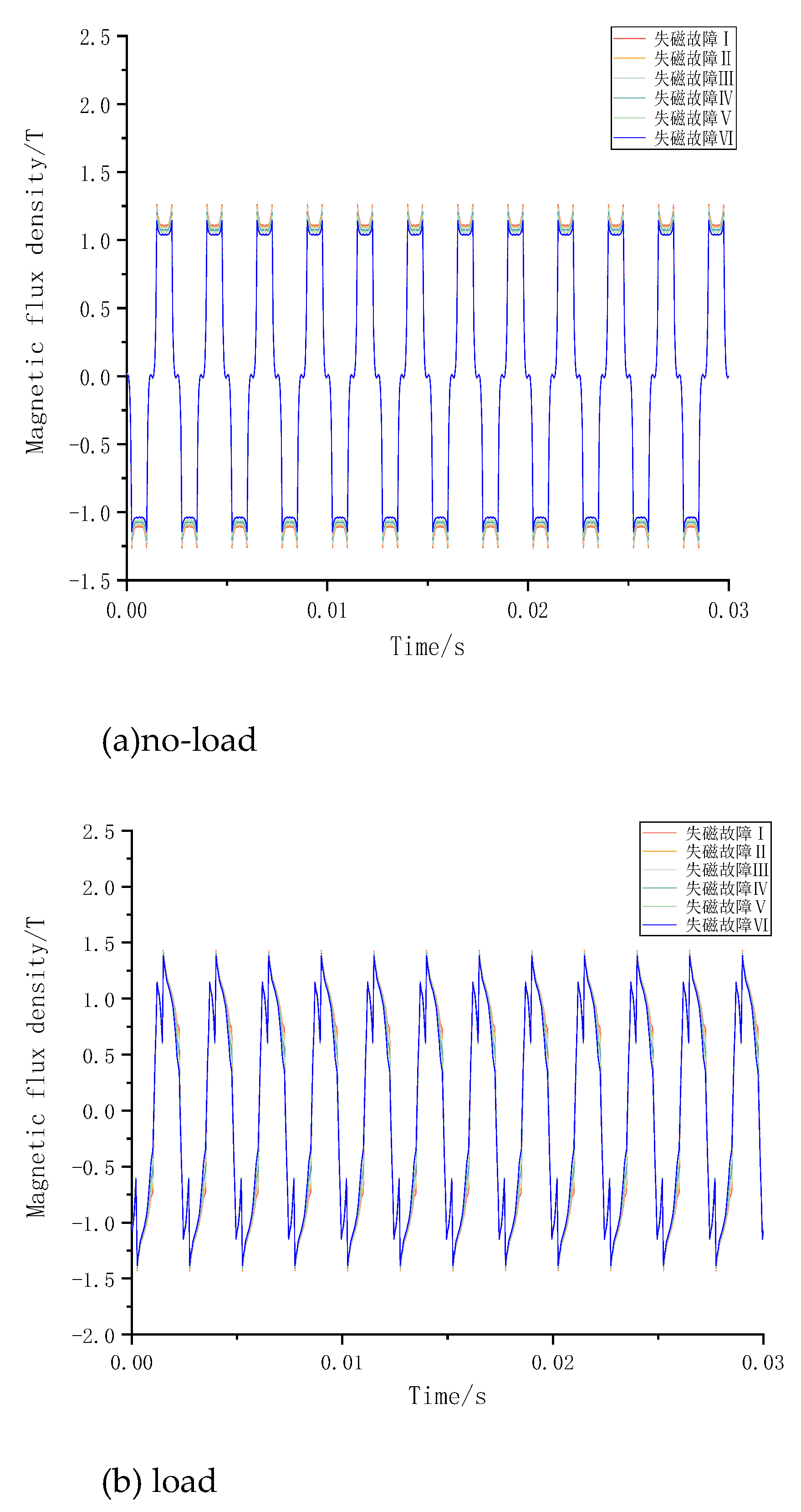
Figure 17.
Mean value of air gap magnetic density.
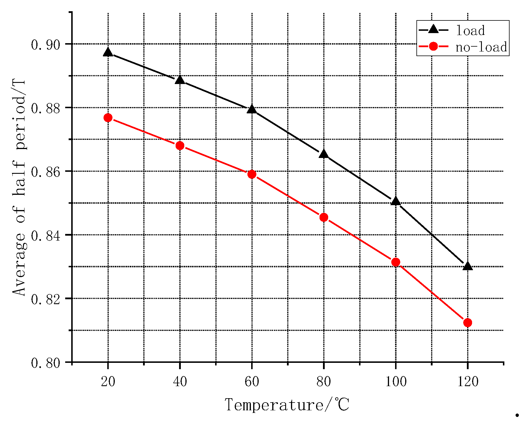
Figure 18.
Induced voltage.
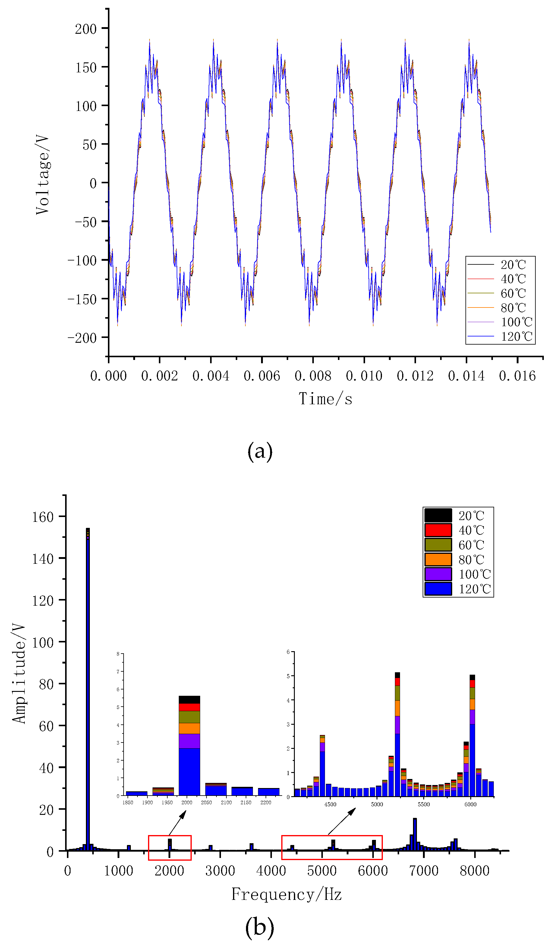
Figure 19.
Torque.
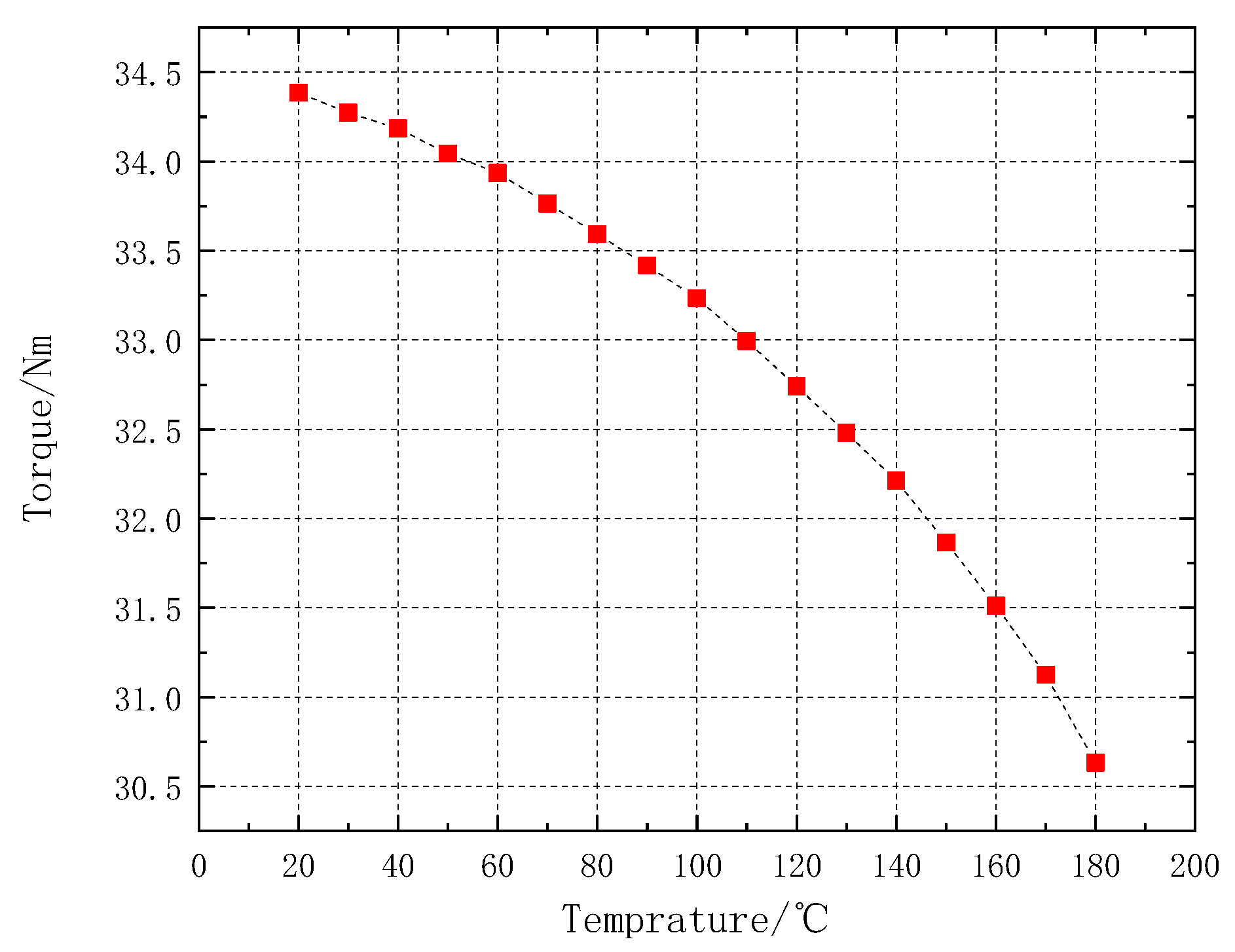
Figure 20.
Frequency of magnetic density.
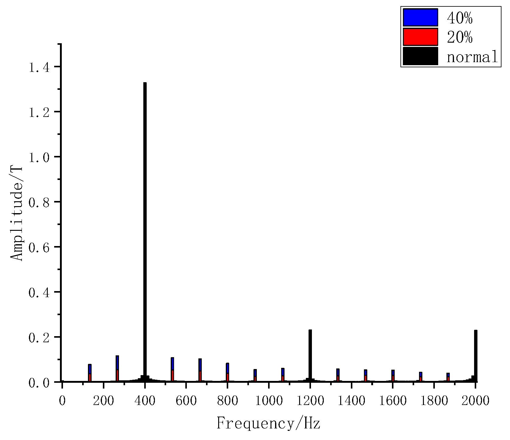
Figure 21.
Induced voltage.
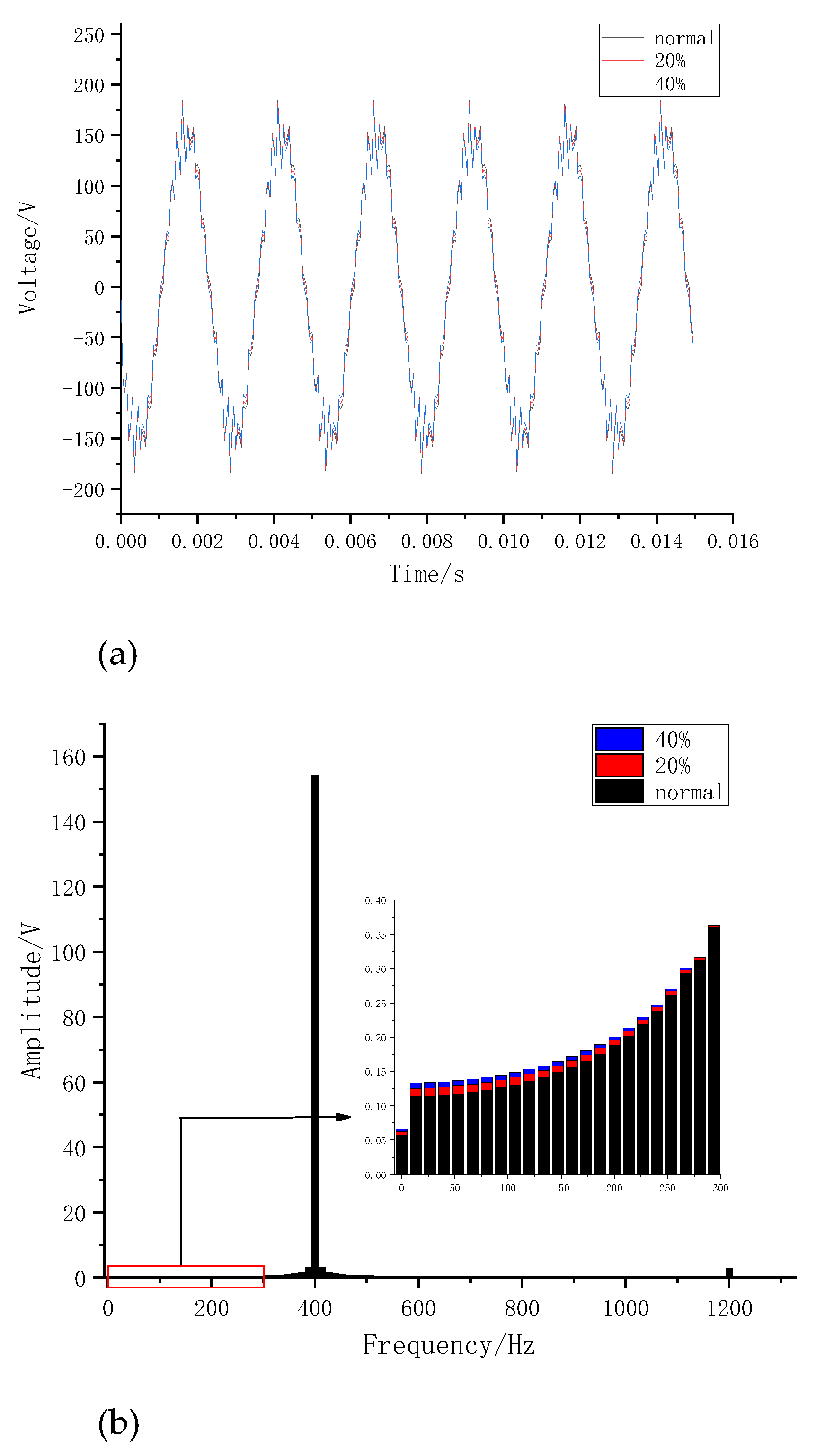
Figure 22.
Torque.
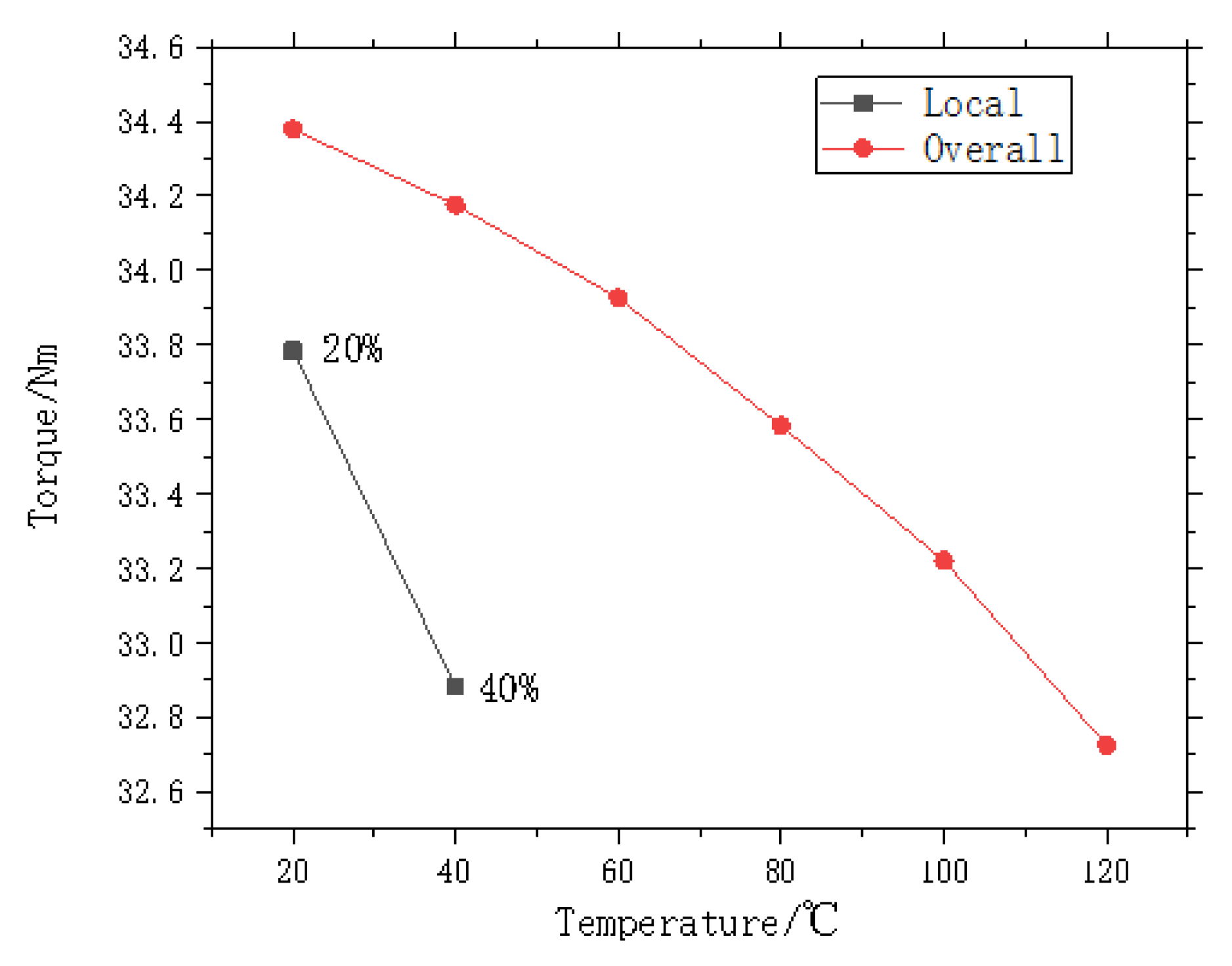
Figure 23.
DBN.
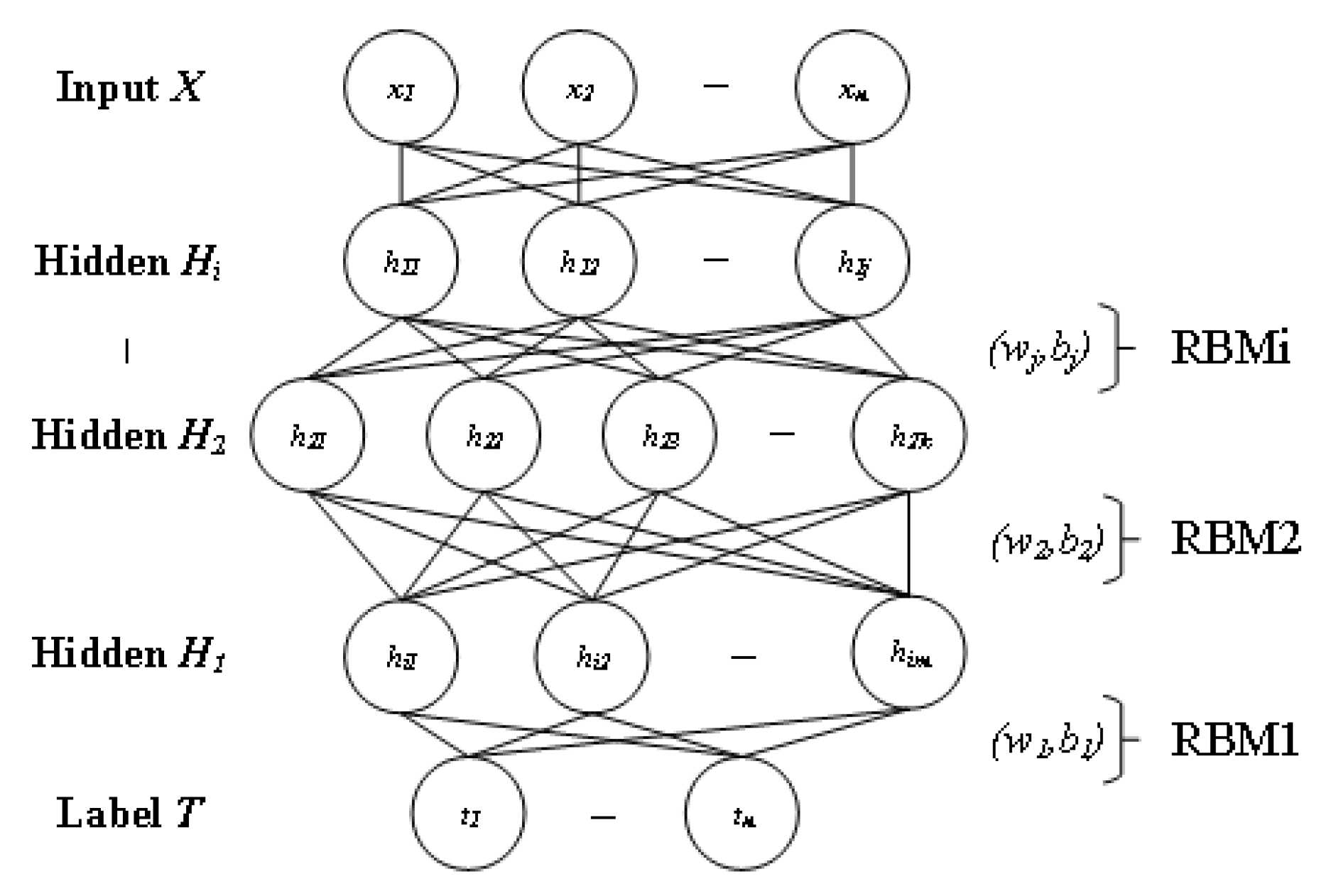
Figure 24.
Noise effect.
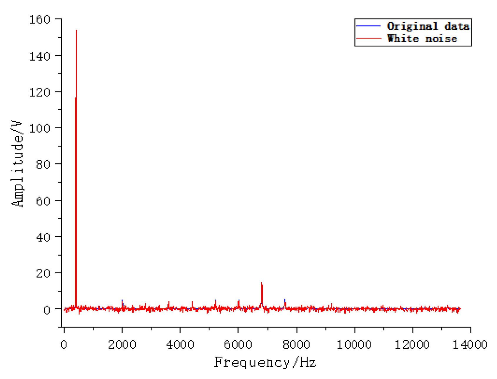
Figure 25.
Diagnostic flow chart.
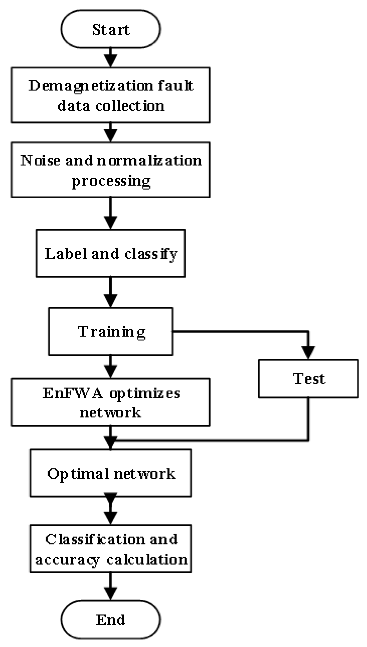
Figure 26.
Diagnostic result.
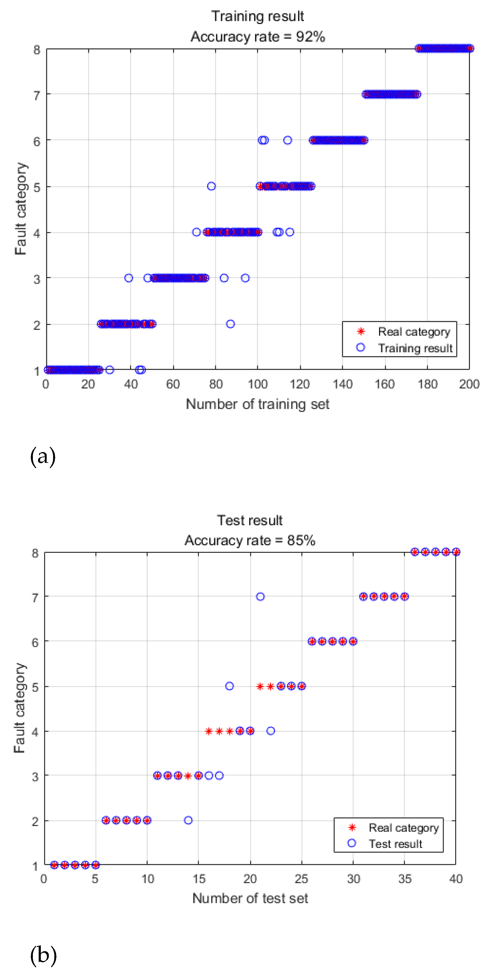
Table 1.
Main parameters.
| Parameter | Data | Parameter | Data |
|---|---|---|---|
| Rated voltage(V) | 200 | Rotor outer diameter(mm) | 189.4 |
| Notch width(mm) | 3.68 | Air gap width(mm) | 0.3 |
| Rated speed(RPM) | 8000 | Number of poles | 6 |
| stator outer diameter (mm) | 296 | inner diameter of stator (mm) | 190 |
| Winding pitch (slots) | 6 | Stator slots | 54 |
| PM thickness (mm) | 5.6 | Notch depth (mm) | 1.21 |
Table 2.
Harmonic amplitude of three phase back electromotive force under no-load operation.
| Frequency | U | V | W |
|---|---|---|---|
| f | 132.651 | 128.736 | 128.963 |
| 3f | 2.897 | 1.562 | 1.379 |
| 5f | 4.439 | 2.613 | 1.83 |
| 7f | 0.577 | 4.049 | 4.137 |
| 9f | 3.282 | 1.528 | 1.846 |
| 11f | 0.588 | 1.841 | 1.688 |
| 13f | 3.932 | 2.22 | 1.742 |
| 15f | 3.818 | 2.238 | 2.544 |
Table 3.
Harmonic amplitude of U phase.
| Frequency | Amplitude | Percentage |
|---|---|---|
| f | 132.651 | 100% |
| 3f | 2.897 | 2.184% |
| 5f | 4.439 | 3.346% |
| 7f | 0.577 | 0.435% |
| 9f | 3.282 | 2.474% |
| 11f | 0.588 | 0.443% |
| 13f | 3.932 | 2.964% |
| 15f | 3.818 | 2.878% |
Table 5.
Fluid physical parameter.
| Parameters | value | value |
|---|---|---|
| Altitude(m) | 0 | 5000 |
| Density/(kg/m 3) | 1.225 | 0.736 |
| Specific Heat Capacity /(J/kg·K) | 1005 | 1005 |
| Thermal conductivity /(W/m·K) | 0.0257 | 0.0243 |
| Thermal diffusivity /(m2/s) | 2.09e-5 | 3.34e-5 |
| Dynamic viscosity /(Ns/m2) | 1.802e-5 | 1.628e-5 |
Table 6.
Overall demagnetization fault.
| PM temperature/℃ | Fault number | Fault label |
|---|---|---|
| 20 | Overall demagnetization fault Ⅰ | 1 |
| 40 | Overall demagnetization fault Ⅱ | 2 |
| 60 | Overall demagnetization fault Ⅲ | 3 |
| 80 | Overall demagnetization fault Ⅳ | 4 |
| 100 | Overall demagnetization fault Ⅴ | 5 |
| 120 | Overall demagnetization fault Ⅵ | 6 |
Table 7.
local demagnetization fault.
| Degree | Fault number | Fault label |
|---|---|---|
| 20% | Local demagnetization fault Ⅰ | 7 |
| 40% | Local demagnetization fault Ⅱ | 8 |
Table 8.
Harmonic amplitude of air gap magnetic density.
| Frequency | FaultⅠ | FaultⅡ | FaultⅢ | FaultⅣ | FaultⅤ | FaultⅥ |
|---|---|---|---|---|---|---|
| f | 1.327 | 1.319 | 1.31 | 1.297 | 1.285 | 1.269 |
| 3f | 0.231 | 0.224 | 0.216 | 0.203 | 0.19 | 0.171 |
| 5f | 0.228 | 0.219 | 0.21 | 0.195 | 0.18 | 0.16 |
| 7f | 0.167 | 0.163 | 0.159 | 0.154 | 0.149 | 0.145 |
| 9f | 0.034 | 0.036 | 0.038 | 0.04 | 0.042 | 0.045 |
| 11f | 0.07 | 0.067 | 0.064 | 0.06 | 0.056 | 0.051 |
| 13f | 0.042 | 0.041 | 0.04 | 0.039 | 0.037 | 0.037 |
| 15f | 0.039 | 0.039 | 0.039 | 0.039 | 0.039 | 0.038 |
| 17f | 0.06 | 0.059 | 0.057 | 0.055 | 0.053 | 0.05 |
| 19f | 0.024 | 0.024 | 0.023 | 0.023 | 0.023 | 0.022 |
Table 9.
Harmonic amplitude.
| Fault/Frequency | 133.38 | 266.76 | 533.51 | 666.89 | 800.27 | 933.64 |
| Normal | 0.00166 | 0.00291 | 0.00270 | 0.00157 | 0.00132 | 0.00136 |
| 20% | 0.0362 | 0.0547 | 0.0534 | 0.0488 | 0.0388 | 0.0248 |
| 40% | 0.0778 | 0.116 | 0.108 | 0.102 | 0.0824 | 0.0543 |
Table 10.
Data collection.
| Label | Torque | Induced voltage | Frequency amplitude |
|---|---|---|---|
| 1 | 30´15000 | 30´45000 | 30´3075 |
| 2 | 30´15000 | 30´45000 | 30´3075 |
| 3 | 30´15000 | 30´45000 | 30´3075 |
| 4 | 30´15000 | 30´45000 | 30´3075 |
| 5 | 30´15000 | 30´45000 | 30´3075 |
| 6 | 30´15000 | 30´45000 | 30´3075 |
| 7 | 30´15000 | 30´45000 | 30´3075 |
| 8 | 30´15000 | 30´45000 | 30´3075 |
Disclaimer/Publisher’s Note: The statements, opinions and data contained in all publications are solely those of the individual author(s) and contributor(s) and not of MDPI and/or the editor(s). MDPI and/or the editor(s) disclaim responsibility for any injury to people or property resulting from any ideas, methods, instructions or products referred to in the content. |
© 2025 by the authors. Licensee MDPI, Basel, Switzerland. This article is an open access article distributed under the terms and conditions of the Creative Commons Attribution (CC BY) license (http://creativecommons.org/licenses/by/4.0/).
Copyright: This open access article is published under a Creative Commons CC BY 4.0 license, which permit the free download, distribution, and reuse, provided that the author and preprint are cited in any reuse.


