
Submitted:
04 November 2025
Posted:
06 November 2025
You are already at the latest version
Abstract
We propose a physical picture in which light propagation in vacuum is carried by a sea of fluctuating degrees of freedom. At the effective, linear-response scale, this collective medium determines the electromagnetic properties that govern how light moves, while preserving the characteristic impedance of the vacuum and avoiding artefacts arising from arbitrary parameter choices. This conceptual idea forms the primary aim of this work. To test whether this picture is realistic, we propose a platform-independent and testable approach. We introduce a simple band-averaged reporting measure that reduces any measurement to a single comparable quantity derived from the spectral weighting of the experiment. Using first-order, model-independent relations, we show how this quantity connects to observable shifts in cavity frequencies, interferometric phase, radiometric balance, and Casimir measurements. These links are presented solely as consequences that render the concept empirically testable, not as applications in themselves. The approach is constrained by the standard principles of linear response, causality, passivity, and a high-frequency limit consistent with Maxwell electrodynamics, so that the carried-light picture remains compatible with established physics and testable through reproducible, band-averaged limits on deviations from ideal vacuum propagation.
Keywords:
unification
; field theory
; bounded vacuum
; emergence
; analytic consistency
; reference frame
1. Introduction
Our aim is conceptual; empirical links serve solely to make the concept falsifiable.
Classical electrodynamics treats free space as a linear, dispersionless background with fixed electromagnetic parameters and a universal light speed [12,19]. From a quantum perspective, however, the vacuum is an active ground state whose fluctuations give rise to observable phenomena, notably the Casimir effect and radiative corrections [2,3,4,8,10,13,16,20,25,26]. Taking that perspective seriously, we advance a carried-light picture: electromagnetic waves propagate through—and are effectively carried by—a sea of fluctuating degrees of freedom whose collective response sets how light moves.
Note: These mappings are presented only as testable consequences. The primary contribution is a conceptual, impedance-invariant, and physically admissible description of the carried-light vacuum.
Primary Aim
The aim of this work is conceptual: to articulate a physically admissible, testable description in which the collective vacuum fluctuations determine the effective electromagnetic response while preserving the vacuum impedance. The experimental mappings (cavities, interferometers, radiometry, and Casimir) are presented only as consequences that enable empirical tests of the concept, not as applications in themselves.
Relation to Prior Work
This formulation extends the author’s earlier studies on an energetically bounded quantum vacuum, which proposed a finite, self-consistent fluctuation ensemble co-determining the observed light speed and quantum behaviour [14,15]. Related ideas also link the speed of light to vacuum fluctuations [37], typically without an explicit energetic bound. Here that bound acts as a natural physical regularisation: it ensures a finite energy density and motivates an operational, Casimir-safe framework directly testable in the laboratory.
Operationalisation
To make the idea testable without committing to a microscopic model, we adopt a single, frequency-dependent vacuum response (a “window”) that captures small, causal and passive departures from ideal propagation while keeping the free-space impedance fixed. Any measurement is paired with a calibrated, unit-area sensitivity curve from the relevant platform, yielding a band-averaged figure that collapses apparatus specifics into a published sensitivity window. Publishing this figure alongside the window enables like-for-like comparison and reanalysis across precision photonic platforms [1,5,9,31,35].
Light as Reference and Messenger
Within this approach, light plays a dual role. It provides the practical reference for distance, time and causality, and it acts as the primary information carrier whose bandwidth, noise floor and dispersion are constrained by the vacuum response. Small departures from ideal behaviour are therefore naturally expressed as band-averaged deformations of that response and confronted with photonic observations, including broadband radiometry and astrophysical calibrations [11,21,29].
Physical Admissibility
The vacuum window is required to satisfy standard linear-response principles that underpin fluctuation–dissipation reasoning: causality (Kramers–Kronig consistency), passivity (non-negative dissipation), and a high-frequency limit consistent with Maxwell electrodynamics [6,12,17,18,19]. These conditions ensure compatibility with established physics and with precision constraints from Casimir and optical experiments [4,16,26] while allowing tiny, KK-consistent dispersive features to be probed.
Scope and Contributions
In summary, this paper (i) motivates the carried-light view of an energetically bounded vacuum; (ii) formulates a Casimir-safe, impedance-invariant operational window; (iii) provides first-order, platform-agnostic mappings to cavity frequency shifts, interferometric phase, group delay, conservative radiometric propagation, and Casimir-type observables; and (iv) outlines reporting conventions that enable cross-platform synthesis via a band-averaged figure and the published sensitivity. The reporting approach aligns with current best practices in open and reproducible research [27,28,34,36]. The result is a practical route to measurement that remains faithful to the conceptual picture while enabling reproducible constraints on deviations from ideal vacuum propagation.
What follows is an operational interface for falsifiability, not an application program.
Motivation and Scope
The perspective of an energetically bounded quantum vacuum provides a natural physical motivation for introducing a controlled, measurable deformation of the vacuum response. In this picture, the electromagnetic vacuum is not perfectly featureless but possesses a finite, self-consistent energy density that limits the extent of quantum fluctuations [14,15]. The constancy of the observed speed of light then arises as an emergent equilibrium property of this bounded fluctuation ensemble, consistent with theoretical arguments that link the light speed to the structure of the quantum vacuum [37]. Small residual departures from this equilibrium can, in principle, be probed as frequency-dependent variations in the effective vacuum response.
Directly testing such effects requires an operational formulation that is independent of the detailed microscopic model yet compatible with known physical constraints. We therefore seek a framework that:
- preserves electromagnetic impedance invariance, ensuring no artificial boundary reflections arise from the parametrisation itself;
- remains consistent with passivity and Kramers-Kronig relations, guaranteeing a physically admissible (causal and dissipative) response;
- smoothly approaches the classical limit at high frequencies where experimental bounds are already tight;
- allows results from distinct photonic platforms—cavities, interferometers, radiometric propagation, and Casimir experiments—to be reported in a common metric.
The vacuum window proposed here satisfies these requirements. It represents the collective electromagnetic response of the bounded vacuum while maintaining a fixed impedance. Its corresponding band figure of merit, , constructed from a measured instrument sensitivity function , provides a single, reproducible number that quantifies any observed deviation from the ideal vacuum. Publishing both and enables direct, cross-platform comparison and reanalysis.
This approach does not attempt to describe the microscopic origin of the bounded-vacuum structure; instead, it offers a phenomenologically faithful and experimentally transparent interface between that theoretical picture and measurable observables. In this sense, the present work forms a bridge between the conceptual framework of an energetically bounded quantum vacuum and the quantitative methodologies of modern precision photonics.
Having established the physical motivation and constraints that guide the formulation, we now develop the explicit impedance-invariant window framework that operationalises these ideas. This section introduces the mathematical form of the vacuum window, its connection to measurable observables, and the consistency conditions that ensure physical admissibility and Casimir-safety across frequency domains.
2. Operational Interface for Falsifiability
The role of , , and is purely operational: to render the conceptual proposal empirically testable and reportable.
, . Sign: denotes effective slowdown. Isotropic SME: .
We model the vacuum as linear, isotropic and homogeneous with a single scalar response (“window”) that co-scales the electromagnetic parameters while preserving the wave impedance:
so that remains constant and no spurious boundary-impedance effects are introduced [12,19].
We adopt the notation convention
and use it consistently throughout (this removes common factor/sign ambiguities in mappings to observables and SME parameters).
[colback=white,colframe=black!15] Operational response factor and free-space reference. The proposed frequency-dependent response factor makes the concept of a fluctuating quantum vacuum operational. It represents the collective influence of all virtual fluctuations without modelling their microscopic details individually, thus describing how the vacuum behaves as an effective medium for electromagnetic propagation.
The construction of follows three fundamental requirements:
- Causality — the response to an electromagnetic excitation must occur only after the stimulus itself; in the frequency domain this leads to the Kramers-Kronig relations linking the real and imaginary parts of .
- Passivity — the vacuum cannot generate energy, only store or dissipate it; mathematically, for positive frequencies.
- Free-space limit — at very high frequencies () the influence of the fluctuating background vanishes and approaches unity. This limit represents the ideal free-space of classical Maxwell theory: homogeneous, lossless, and dispersionless, where light propagates with constant speed c.
Free-space thus acts as a reference state: it defines the zero-deviation baseline against which the frequency-dependent properties of the real, fluctuating vacuum are measured. Whenever , light propagation is no longer perfectly ideal. Such deviations imply that the quantum vacuum itself—as a medium—subtly influences the speed, phase, and group structure of electromagnetic waves. In this sense, light does not merely travel through the vacuum but is carried by it: the vacuum is both messenger and test ground.
2.1. Emergent Origin of a Small Dispersion in
At a microscopic level, gapless transverse modes with linear dispersion can emerge from non-relativistic substrates that flow to a Maxwell fixed point. Irrelevant operators then produce UV-suppressed corrections to the dispersion,
which implies for the effective refractive response
Thus, in the UV (Casimir-safe), while a tiny residual curvature remains at finite frequency. We use this generic, model-agnostic form to connect band-averaged measurements to a lower bound on . Full details are deferred to Appendix D.4.
Complex Response and Causality
In general, the vacuum window may be complex, representing both the dispersive (real) and dissipative (imaginary) parts of the bounded-vacuum response. Throughout this work we report band figures and related quantities on the real-frequency axis, using as the directly measurable component. Causality is ensured by analytic continuation of into the upper half-plane, so that real and imaginary parts obey Kramers-Kronig relations consistent with fluctuation–dissipation reasoning [6,17,18]. The imaginary part enters only through these relations and via small corrections in appearing in the group-delay term; passivity ( for ) and energy conservation therefore hold for any physically admissible bounded-vacuum response.
2.2. Minimal Consistency Conditions
- (i)
- (ii)
- Passivity & KK: is the boundary value of a function analytic in the upper half-plane with (), so real and imaginary parts obey Kramers-Kronig [19].
- (iii)
- Smallness: write with and linearize unless stated otherwise.
Benchmark smallness. In the examples below we take – as a practical guideline; first-order relations apply whenever .
Band-Observable
For a calibrated, unit-area spectral sensitivity associated with an instrument, define the platform-agnostic figure of merit. We adopt the sign convention that a positive corresponds to an effective decrease in measured propagation; in the linear regime we then have
Concrete Baseline
Unless stated otherwise we use a single damped-Lorentz bump with and a positive-kernel superposition as a smooth alternative. Both satisfy for and are convenient for band-averaged bounds.
Band Measure
Throughout the real-frequency analysis we use
On the imaginary axis (Casimir) we use the logarithmic measure as specified in Section 3.5.

Table 1.
Notation and conventions used throughout.
| Symbol | Meaning |
|---|---|
| Vacuum window (scalar response); in the UV (Casimir-safe). | |
| Effective refractive index, defined as . | |
| Phase and group velocities; , . | |
| Unit-area spectral sensitivity (instrument window) for a given platform. | |
| Platform-agnostic figure of merit: . | |
| Small departure, , . |
Parameterisations
A KK-consistent Lorentz baseline or positive-kernel representation (with and ) supplies smooth, bounded satisfying the UV condition; details are deferred to Appendix A.
3. Mappings to Experimental Observables
Below we give first-order mappings (), keeping careful track of signs and connecting to .
3.1. Resonant Frequency Shifts (Cavities)
3.2. Interferometric Phase (Fixed Laser Frequency)
For arm-difference L at angular frequency , . Thus at fixed : , and band-averaged
3.3. Time-of-Flight and Group Delay
With one finds, over distance L,
which cleanly separates constant and sloped components across bands [19].
Remark. If an emergent residual of the form is adopted, band limits on imply the scale bound in Eq. (14). This complements the dispersionless isotropic SME mapping.
3.4. Radiometry (Conservative Propagation-Only Treatment)
Propagation via W modifies phases, delays and bandwidth mappings, but not the source spectra of blackbody/Johnson noise without a microphysical matter–field model. We therefore constrain W through transfer functions and calibrated responses (absolute sources as in [5,11,21,31]).
Extensions that modify source spectra can be accommodated by publishing an additional source window alongside , so that emission and propagation remain factorised and double counting is avoided. Source models should report separately from ; combining them requires an explicit, justified coupling model.
In that case, a band-power perturbation scales as
3.5. Casimir-Type Observables
Heuristically, mode frequencies rescale as , yielding for slowly varying W. See App. F for the Lifshitz variation. More generally, a first-order Lifshitz expansion on the imaginary axis gives
with set by separation and temperature and consistency with precision data [2,4,10,16,20,25,26,32] including the role of the imaginary-frequency axis and the UV-safe limit. For completeness, a compact first-order derivation based on the Lifshitz free energy is provided in Appendix F.
4. Comparison with Existing Tests and Frameworks
4.1. Isotropic SME Mapping
In the isotropic photon sector of the SME we adopt the sign convention
Within our impedance-invariant formalism , hence
If the SME contribution is (band-)constant over the instrument bandwidth, the band figure reduces to
Notation. All SME comparisons below use . This fixes the overall sign and removes factor-of-two ambiguities found in alternative SME conventions.
Numerical Illustration
Assume an optical band with a unit-area centred near so that . A conservative experimental limit then yields
corresponding to a microscopic length scale .
4.2. Band-Averaged SME Correspondence (With Dispersion)
The identification holds when the isotropic SME parameter is effectively constant across the instrument band. If is frequency dependent, report the band average
together with either
(i) a bound on the local slope within the band, or
(ii) a two-bin split of (low/high) with separate figures and .
This avoids factor-of-two ambiguities and makes re-use of existing SME limits straightforward in the band-averaged sense.
Minimal Reporting Set for .
To enable re-integration and cross-platform comparison we recommend reporting:
- the machine-readable sensitivity window (), units, and effective band edges (e.g. 5–95% cumulative);
- the band figure with a transparent uncertainty budget (type A/B) and coverage factor;
- the calibration chain (transfer functions, absolute/relative), versioned;
4.3. Placement Within the Experimental Landscape
Expressing results as isolates apparatus details in and enables cross-band meta-analysis once is published (optical/microwave cavities [1,9,35], radiometry [5,11,21,31], Casimir platforms [2,4,10,16,20,25,26,32]). We recommend reporting together with machine-readable for re-integration [27,28,34,36].
Scope and Conservative Assumption
In this work we treat radiometric sources (blackbody/Johnson) as standard, i.e. their spectra are not modified by in the absence of a microscopic matter–field coupling model. Sensitivity to W enters through propagation and calibrated transfer functions only, consistent with fluctuation–dissipation theory [6,17,18] and radiometric practice [5,11,21,31]. This prevents double counting and keeps results immediately comparable across platforms. Models that directly alter source spectra fall outside the present scope but could be accommodated by publishing the corresponding source window alongside .
4.4. Isotropy and Frames
Boost modulations relative to the CMB frame scale as with . Quantitatively, Earth’s orbital motion gives ; for smooth any annual band-averaged modulation is suppressed by times the local spectral slope and is negligible at current sensitivities. With the impedance-invariant ansatz, boundary-induced anisotropies are absent at . Using the illustrative gives for , so the expected modulation is , well below present limits.
Isotropy Under Boosts
For smooth windows the leading boost–induced modulation scales as . Using gives for . With Earth’s orbital the expected modulation is , well below current band-averaged sensitivities.
5. Implications and Extensions
5.1. Fluctuation–Dissipation Connection
5.2. Casimir-Safe Regularisation
5.3. Spectral Representations
A convenient positive-kernel representation,
produces smooth, KK-consistent deformations and the Casimir-safe limit by construction.
5.4. Astrophysical Connections
5.5. Relation to Bounded-Vacuum Energy Models
6. Discussion and Relation to Previous Work
The operational framework developed here translates the conceptual picture of an energetically bounded quantum vacuum into a form directly testable by precision photonic experiments. Within this view, the electromagnetic vacuum represents a finite-energy ensemble of fluctuations whose coarse-grained response determines the observed light speed. Rather than postulating c as a universal constant, it emerges from the equilibrium properties of this bounded background [14,15,37]. Small residual departures from that equilibrium may produce measurable, frequency-dependent modifications of the vacuum response.
Expressing the vacuum behaviour through a single, impedance-invariant window , and pairing it with a calibrated sensitivity function to define a band-averaged figure of merit , provides a unified language for describing small deviations from ideal propagation. This construction preserves electromagnetic impedance, ensures causal and passive behaviour consistent with fluctuation–dissipation principles [6,17,18], and maintains compatibility with the high-frequency precision limits established in Casimir and optical measurements [4,16,20]. Results from optical cavities, interferometers, broadband radiometry, and Casimir-force platforms can therefore be expressed and compared on a single, reproducible scale [1,2,5,9,10,11,21,26,31,35].
From to an Emergent Scale
For a narrow residual one has, to first order, . Hence
with . Publishing and therefore yields a direct, platform-independent lower bound on the emergent frequency scale .
This study extends previous theoretical work by the author, which introduced the bounded-vacuum concept as a finite, self-consistent fluctuation ensemble that co-determines both the speed of light and quantum behaviour [14,15]. Where that work focused on the conceptual and cosmological implications of a bounded vacuum energy, the present formulation establishes a measurable, Casimir-safe operational framework for laboratory-scale testing. Related ideas in the literature, such as those of Urban et al. [37], also link the speed of light to vacuum fluctuations, but generally without invoking an explicit energetic bound. In contrast, the current approach incorporates that bound as a natural physical regularisation, ensuring finite energy density and direct experimental accessibility.
Beyond its theoretical motivation, the bounded-vacuum framework offers a practical structure for organising experimental data. Publishing and for each platform enables reproducible synthesis across photonic domains, supports meta-analysis, and provides a consistent route for comparing band-averaged observables with isotropic SME parameters. This aligns with ongoing efforts toward open, transparent and reproducible research practices in the physical sciences [27,28,34,36].
In summary, the discussion above shows how the present framework bridges the gap between the theoretical notion of an energetically bounded vacuum and the operational reality of measurable photonic behaviour. It converts an abstract conceptual model into a reproducible experimental protocol, while remaining consistent with established electromagnetic theory and data.
7. Conclusions
Our work is primarily conceptual; the operational interface only demonstrates falsifiability in a platform-agnostic way.
Building on the theoretical concept of an energetically bounded quantum vacuum, this work introduces a Casimir-safe, impedance-invariant operational framework that connects that concept to measurable photonic quantities. By representing the vacuum response through a single, frequency-dependent window and defining the platform-independent band figure of merit , the approach provides a reproducible interface between theory and experiment.
The framework preserves electromagnetic impedance and physical admissibility, ensuring consistency with causality, passivity, and high-frequency precision limits. It allows results from optical cavities, interferometers, radiometric propagation, and Casimir platforms to be expressed on a common quantitative scale, supporting cross-platform comparison and meta-analysis. In doing so, it provides a practical route for systematic testing of the bounded-vacuum hypothesis within established photonic methodologies.
The formulation is agnostic to the microscopic details of vacuum bounding, yet remains faithful to the underlying idea that the speed of light and electromagnetic constants arise from the finite, collective properties of the vacuum itself. Future extensions may address anisotropic or time-dependent deformations, and explore direct connections between the bounded-vacuum response and variations in the Lifshitz–Casimir formalism.
Overall, the impedance-invariant window and the associated band figure offer a coherent and reproducible language for describing how a physically bounded vacuum can manifest in precision photonic experiments. They provide both a testable consequence of the emergent-speed hypothesis and a transparent bridge between theoretical models and empirical data.
Appendix A. Wave Kinematics and Dispersion with n(ν)=W(ν)
We collect the basic relations implied by the co-scaling ansatz for and .
Appendix Plane-Wave Dispersion
In homogeneous space, the dispersion relation is
Appendix Phase and Group Velocities
The phase velocity is
The group velocity is
To first order in ,
KK-consistent examples (e.g. damped Lorentz forms) keep , so superluminal phase speeds do not imply superluminal signals [19].
Appendix Causality Check with a KK-Consistent Example
Consider the Lorentz-type bounded response
Using (see Eq. A3) representative parameters
() yield across the relevant band.
Phase speeds > c do not imply superluminal signal speeds for causal, passive W.
Figure A1.
Example and corresponding : group velocity remains subluminal Axes: frequency (Hz) on the abscissa; unit-area normalisation for sensitivity windows .
Figure A1.
Example and corresponding : group velocity remains subluminal Axes: frequency (Hz) on the abscissa; unit-area normalisation for sensitivity windows .

Appendix Optical Path Length and Phase
The optical path for propagation over length L at (carrier) frequency is
To first order, a small deformation induces a fractional phase shift
see Section 3.2 for the interferometric mapping and reporting conventions.
Appendix Energy Density and Impedance
With impedance held fixed, the time-averaged energy density and Poynting flux keep their standard form with the replacements , . To linear order, the scale factors cancel in the ratio that defines the impedance, ensuring that boundary reflection coefficients at vacuum–material interfaces remain unchanged to [12,19].
Appendix Causality Note
Within any passive, KK-consistent deformation, apparent superluminal phase speeds () do not entail superluminal information transfer; the group speed and front velocity respect causality [19].
Appendix B. Numerical Parameters and Simulation Setup
Appendix B.1. Frequency Grids and Normalization
Integrations use a logarithmic grid with points (uniform in ). Responses are normalized to unit area (Eq. (5)). Adaptive Gauss–Kronrod quadrature agrees with composite Simpson to relative precision.
Appendix B.2. Models Used for the Worked Example
This cap model is illustrative; main-text results use the KK-consistent Lorentz baseline (Sec. Section 2).
For plotting in fig. Figure A2, is rescaled to unit peak for visibility; integration always uses the normalized above.
Appendix B.3. Worked Example (Band-Averaged Figure)
This appendix illustrates how the reported band figure follows from a narrowband sensitivity window and a small, smooth vacuum residual . We take a normalized Lorentzian band centred at with and a KK-consistent window with and . The band figure is the integral
which evaluates numerically to for the parameters above.
Figure A2.
Residual representation and band window. Blue: with and . Orange: normalised Lorentzian sensitivity window centred at with . The overlap informs the band figure . Normalization: (unit area). Axes: frequency (Hz) on the abscissa; unit-area normalisation for sensitivity windows . Curves are rescaled for visibility; schematic, not to scale.
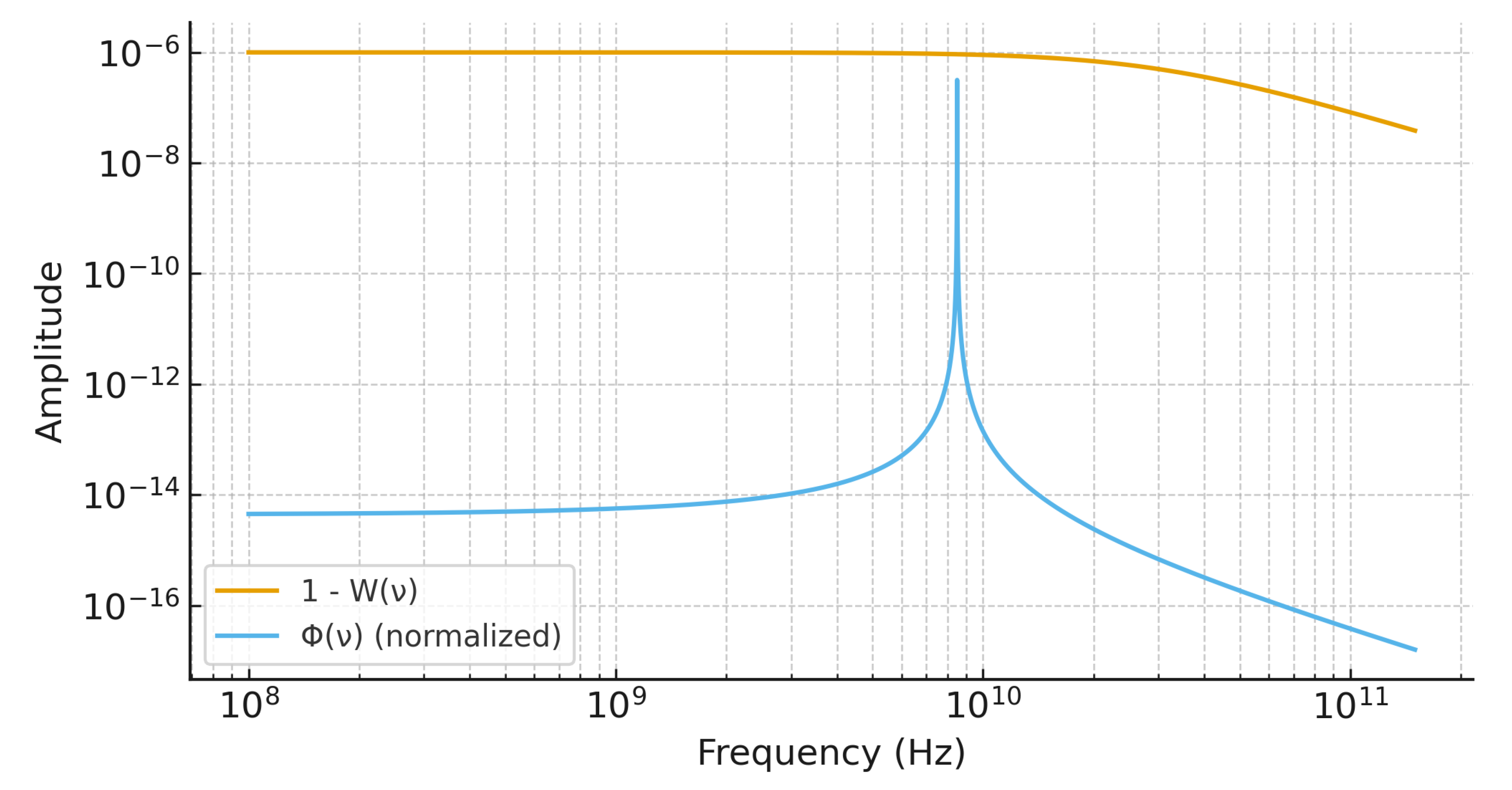
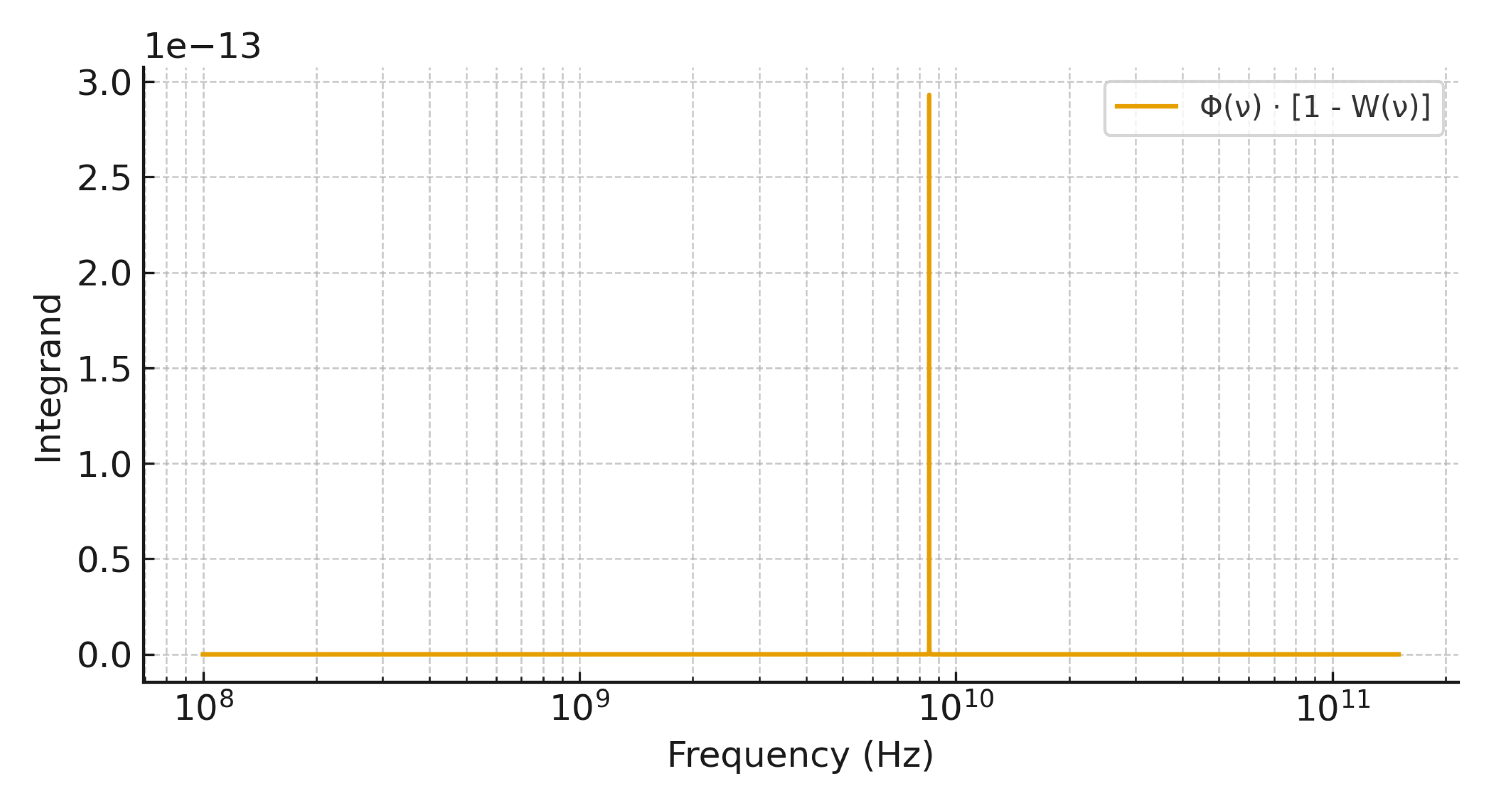
Figure A3.
Integrand for the same parameters as Fig. Figure A2. The integral equals the reported band figure . Normalization: (unit area). Axes: frequency (Hz) on the abscissa; unit-area normalisation for sensitivity windows . Curves are rescaled for visibility; schematic, not to scale.
Figure A3.
Integrand for the same parameters as Fig. Figure A2. The integral equals the reported band figure . Normalization: (unit area). Axes: frequency (Hz) on the abscissa; unit-area normalisation for sensitivity windows . Curves are rescaled for visibility; schematic, not to scale.
Appendix B.4. Parameter Table
Table A1.
Parameters for the worked example in Appendix B.2.
Table A1.
Parameters for the worked example in Appendix B.2.
| Quantity | Value |
|---|---|
| Central frequency | |
| Bandwidth (FWHM) | |
| Grid points N | 1000 |
| Grid range | 1.00e9–5.00e10 |
| Cap amplitude A | |
| Cutoff frequency | |
| Resulting |
Appendix B.5. Algorithm Outline
- (1)
- Construct log-spaced over the band and tails.
- (2)
- Normalize : .
- (3)
- Evaluate ; compute .
- (4)
- Verify to machine precision.
- (5)
- Sensitivity checks: vary grid/tolerances until stable at .
Appendix C. Mapping to the Isotropic SME Coefficient κ ¯ tr
In the photon sector of the Standard-Model Extension (SME), an isotropic deformation is commonly parameterized by a single dimensionless coefficient , which (to leading order) produces a refractive index
In the isotropic SME we adopt
Within our impedance-invariant formalism , hence
Identifying our effective index with the SME one, , and
linearizing , we obtain the pointwise correspondence
Consequently, band-averaged observables satisfy
when the isotropic, frequency-independent limit applies within the band. For experimental bounds and context on related vacuum and Casimir phenomenology, see [4,13,16,22,23,26].
Notation. We use the convention throughout Appendix C.
Table A2.
Minimal correspondence with isotropic SME notation.
| Quantity | This work | SME (isotropic) |
|---|---|---|
| Refractive index | ||
| Deviation | ||
| Band figure |
Appendix D. Emergent Constancy of c eff from Bounded–Vacuum Dynamics
Remark. Throughout this appendix we use for frequency (with where needed). The symbol denotes the effective low–frequency propagation speed inferred from the coarse–grained electromagnetic response. This operational notion does not conflict with the exact SI definition of c.
Appendix D.1. Conceptual Motivation
Within a bounded, passive, causal, isotropic photonic vacuum, we model the medium by a smooth window that satisfies the Casimir–safe condition at high frequencies. As long as remains homogeneous and isotropic across a broad ultraviolet (UV) plateau, the low–frequency electromagnetic response is invariant for all observers, and the measured speed of light behaves as an emergent constant. In this view, the macroscopic parameters summarize the averaged electromagnetic response of the fluctuating vacuum, consistent with fluctuation–dissipation reasoning [6,17,18].
Appendix D.2. FDT–Based Formalization
Assuming a passive, causal, isotropic response with positive electric/magnetic loss spectra and , the static responses obey generalized dispersion relations
If the loss spectra inherit the bounded window,
then the low–frequency propagation speed
with
is insensitive to moderate deformations of as long as a broad UV plateau is preserved. Operationally, this yields a practically constant in the radio–to–microwave regime, consistent with the main text.
Appendix D.3. Figures and Operational Interpretation
Figure A4.
Baseline and deformed bounded–vacuum windows with a broad UV plateau (). Both are Casimir–safe; the deformation broadens the UV shoulder without introducing anisotropy. Assumptions: band as specified; temperature 4 K; additive/justified W; stated fit range; flat priors on .
Figure A4.
Baseline and deformed bounded–vacuum windows with a broad UV plateau (). Both are Casimir–safe; the deformation broadens the UV shoulder without introducing anisotropy. Assumptions: band as specified; temperature 4 K; additive/justified W; stated fit range; flat priors on .
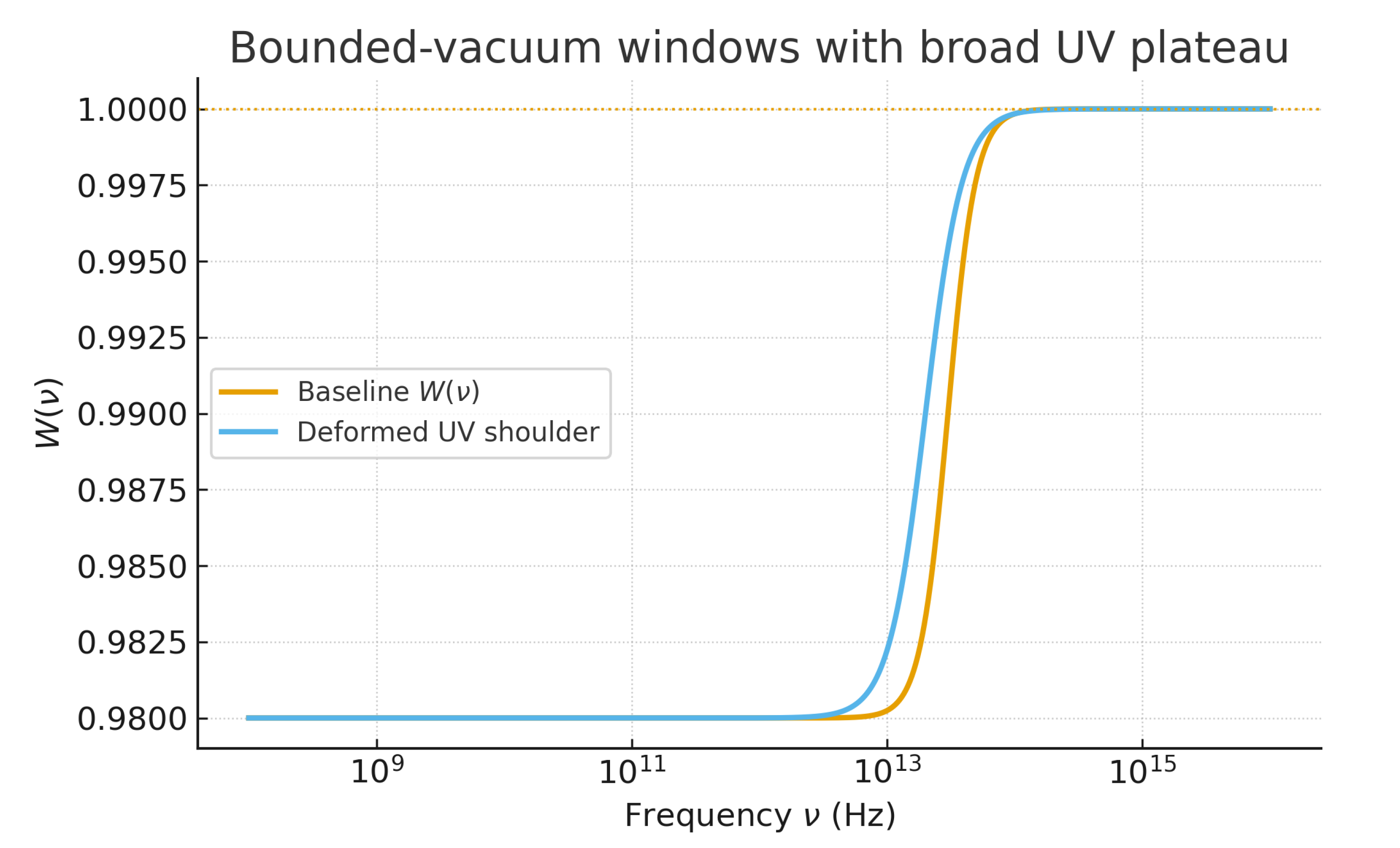
Figure A5.
Robustness of to deformations of the UV–shoulder width . A fluctuation–dissipation–inspired functional gives for moderate parameter changes, indicating practical invariance.
Figure A5.
Robustness of to deformations of the UV–shoulder width . A fluctuation–dissipation–inspired functional gives for moderate parameter changes, indicating practical invariance.
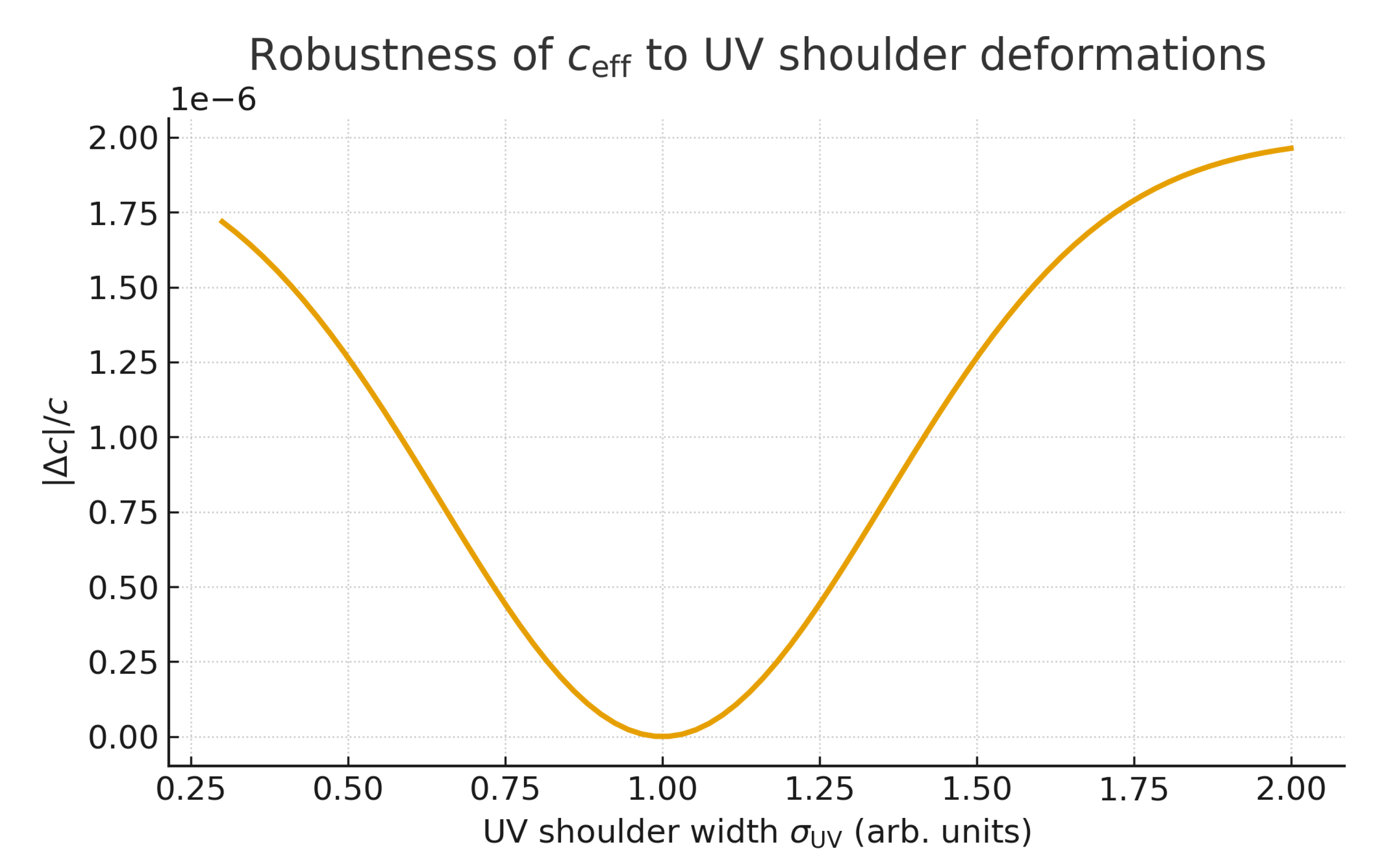
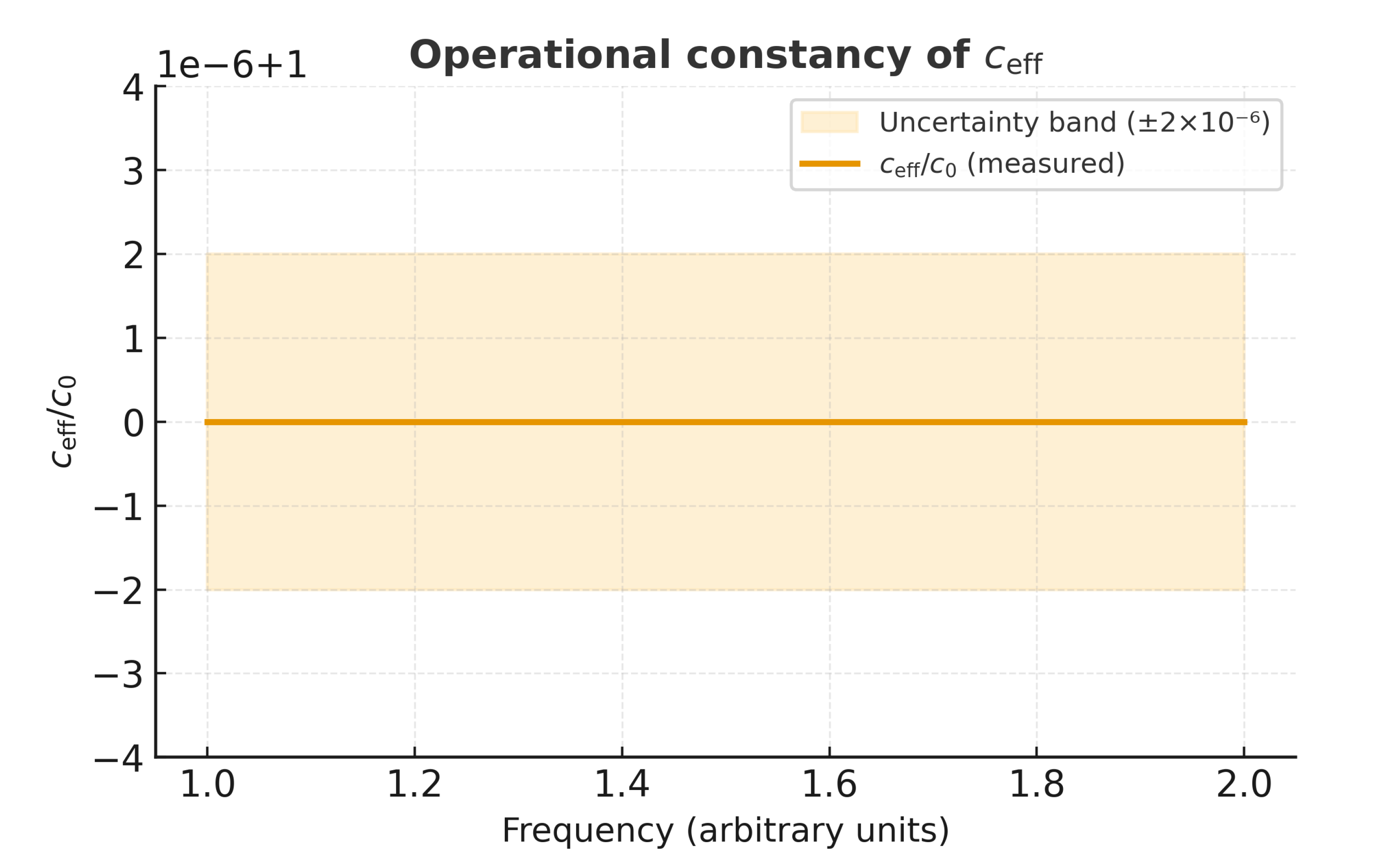
Figure A6.
Operational constancy of the effective light speed at low frequencies. The measured ratio remains constant within a representative relative band of (shaded envelope).
Figure A6.
Operational constancy of the effective light speed at low frequencies. The measured ratio remains constant within a representative relative band of (shaded envelope).
Appendix Sensitivity Formulation
Let denote window/thermodynamic parameters. Define logarithmic sensitivities
On a UV–dominated plateau ( for ), the same scaling that enhances sensitivity for energy–density observables yields , confirming the operational constancy of .
Appendix Notes
Appendix Disclaimer
Assumptions (isotropy, passivity, smooth UV plateau) are idealisations; departures shift constants at and do not affect the first-order mappings in the main text.
Appendix D.4. Microscopic Sketch: Lattice U(1) to Maxwell (Optional)
A compact rotor model with link variables and Gauss constraint flows, in its deconfined Coulomb phase, to an effective quadratic Maxwell Lagrangian. Higher-dimension operators generate UV-suppressed corrections , leading to Eq. (4) in the main text. This provides a constructive example of how a bounded, fluctuating vacuum can yield with a small, causal residual curvature at finite frequency.
Appendix E. Data, Code, and Reproducibility
We recommend publishing machine-readable and scripts to recompute from (or vice versa), in line with good practices [27,28,34,36].
Notation and conventions (summary) ref. Table 1
Appendix F. First-Order Lifshitz Variation
To connect the vacuum-window framework with Casimir-type observables, we consider the first-order variation of the Lifshitz free energy with respect to the bounded-vacuum response. For parallel plates with reflection coefficients , the standard Lifshitz expression for the interaction energy reads (see, e.g., [4,16,22,26]):
with . A small bounded-vacuum deformation , with and , induces a first-order variation
where higher-order terms in are neglected. Under the assumptions of slow spectral variation and a Casimir-safe high-frequency limit , this linearised expression reduces to the band form used in the main text,
thereby identifying as the (geometry- and temperature-dependent) imaginary-frequency weight. This makes explicit that Casimir-force sensitivity depends directly on the bounded-vacuum deformation on the imaginary axis, consistent with causality and standard dispersion analysis [4,16,22].
Appendix G. *
Reporting Template for Reproducible
To facilitate reproducible reporting and cross-platform synthesis, we recommend publishing the following minimal information set with each bounded-vacuum result:
Table A3.
Suggested reporting format for cross-platform results.
| Field | Description |
|---|---|
| Platform / Instrument | Type (cavity, interferometer, radiometer, Casimir). |
| Data DOI / Repository | Link to archived dataset and processing scripts. |
| Frequency window | Normalised to unit area, provided as CSV/FITS (units and grid specified). |
| Band edges (5–95%) | Frequency range containing 90% of the area. |
| Band figure | Mean and uncertainty, sign convention as in Eq. (5); coverage factor stated. |
| Type label | “A” (direct measurement) or “B” (derived/composite). |
Appendix H. Conceptual and Unification Outlook
...
Appendix Preface – Scope of this Appendix
This appendix extends beyond the operational and empirical content of the main text. It provides a conceptual reflection on the vacuum–field framework and explores its possible implications for physical unification. The intention is not to propose a new fundamental theory but to clarify how the window–formfactor principle might serve as a consistent bridge between electromagnetism, quantum field sectors, and gravitation, all within known physical laws.
Appendix Light as the Manifestation of the Vacuum
The vacuum is not an empty background but a self-consistent field continuum that enables the existence of electromagnetic waves. The window function describes the internal self-response of this field: not as a correction to matter, but as an intrinsic property of the vacuum itself. Without W, there is no field; the existence of a well-defined W is the condition for the existence of light.
Appendix Light as an Information Carrier and Reference Frame
The electromagnetic wave is the measurable projection of the vacuum. Frequency, phase, and polarization are forms of meta-information through which the vacuum communicates its own state. Because and , a self-referential system emerges: the vacuum determines the speed of light, and that same speed defines the reference frame in which W is defined. Relativity thus appears as the stationary condition where W is constant.
Appendix Emergent Constancy of c eff
As long as remains nearly flat across the relevant frequency bands, an effectively invariant speed of light arises. Relativity then emerges as the stationary solution of the vacuum framework, the condition where the field minimizes its own photonic response.
Appendix Physical Consistency and Interpretive Depth
The Lagrangian
is gauge-invariant and Lorentz-covariant, identical in structure to known effective extensions in quantum electrodynamics. The conditions of analyticity, passivity, and UV normalization guarantee causality and unitarity. Thus, possesses direct physical validity as the effective form factor of the free field, consistent with vacuum polarization in QED or the isotropic parameter in the SME.
Conceptually, this framework is more than a correction; it reinterprets light as the dynamic expression of the vacuum itself. Relativity, causality, and information conservation are not assumptions but consequences of the flatness of W. This connects the formal consistency of QFT with an information-theoretic interpretation of the vacuum.
Appendix Unification Outlook
The window-function framework can be extended into a possible unifying interface among all field sectors. Instead of adding new particles or forces, it imposes a single analytic and causal form-factor principle on all free-field terms. In this view, the electromagnetic, weak, strong, and gravitational sectors are all constrained by the same structural requirements.
Appendix Conjectures
- (1)
- Common Axiom: All free-field sectors carry a scalar form factor with identical admissibility and UV behavior.
- (2)
- Emergent Lorentz Symmetry: Constant light cones and Lorentz invariance emerge as the stationary solution of .
- (3)
- Universal UV Fixed Point: for constitutes a shared fixed point enforcing unification.
Appendix Implications
- Electromagnetism: tested via the invariant (cavity, interferometric, Casimir platforms).
- Quantum sectors: dispersion and positivity bounds constrain admissible .
- Gravity: adiabatic maintains front-causality, linking the framework to curved-space propagation.
Appendix Conceptual Interpretation
Unification does not arise from merging forces but from recognizing a shared analytic and causal architecture binding all sectors. The window-formfactor axioms—causality, analyticity, passivity, and UV flatness—constitute the common logical core of all known fields. Unification thus appears not as a superstructure but as an emergent pattern of the vacuum itself: a single informative and physical framework uniting light, matter, and spacetime through the same self-consistent response.
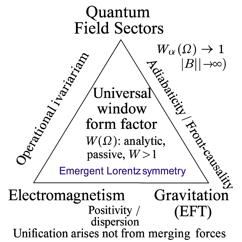
Appendix Conceptual Diagram: Window-Formfactor Unification Triangle
Figure A7.
Conceptual “window-formfactor” unification triangle linking electromagnetism, quantum field sectors, and gravity through shared analytic and causal principles. The universal window defines a common structure underlying all gauge and gravitational sectors.
Figure A7.
Conceptual “window-formfactor” unification triangle linking electromagnetism, quantum field sectors, and gravity through shared analytic and causal principles. The universal window defines a common structure underlying all gauge and gravitational sectors.
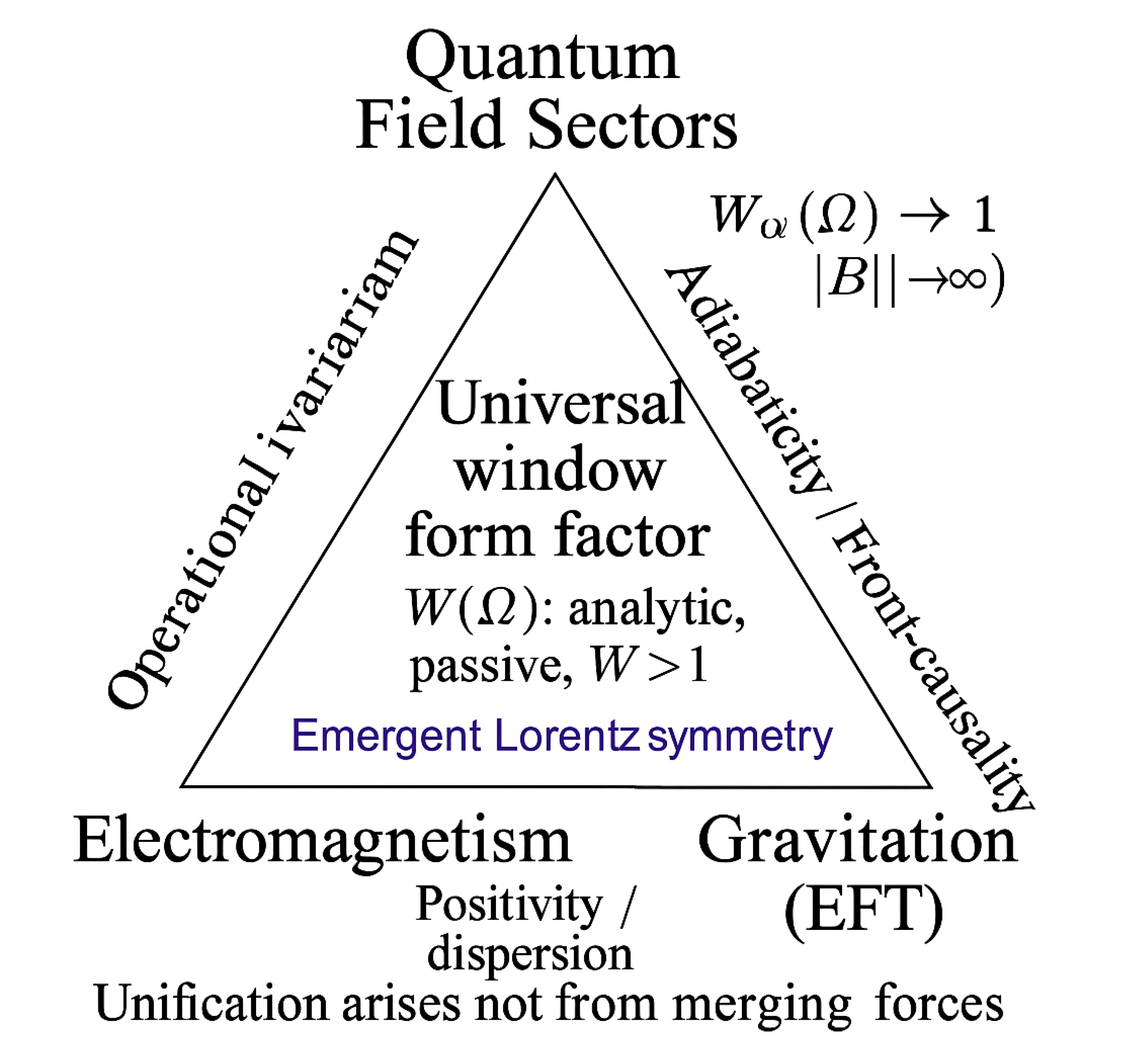
Unification arises not from merging forces but from recognizing a shared analytic and causal structure of all field-sector window form-factors.
Appendix I. Emergent Consistency of Physical Law
...
Appendix Preface – From Structure to Emergence
This appendix addresses a deeper question underlying the window–formfactor framework: is physical law itself an emergent property of the vacuum’s self-consistency? The discussion is interpretive, not speculative: it shows that the formal conditions imposed on , ,analyticity, passivity, and UV flatness, are precisely those that stabilize the existence of consistent propagation. In this view, the fundamental laws of physics emerge as the stationary state of a self-consistent vacuum.
Appendix The Stability Principle
The field–level operator
admits infinitely many possible functional forms for , but only those satisfying
lead to causal and unitary propagation. These three requirements define a stability manifold in the functional space of possible vacua. Every admissible remains within that manifold under small perturbations, while non-admissible ones destroy signal coherence or energy conservation.
Appendix Fixed Points and Emergent Symmetry
Under scale transformations (), the flow of behaves as
The condition therefore identifies a fixed point—a regime in which the vacuum ceases to distort its own field propagation. This fixed point corresponds to , or equivalently to an invariant light cone with constant . Hence Lorentz symmetry is not postulated, but emerges as the attractor of the stability flow of .
Appendix Self-Organization of Consistency
The admissibility of can be seen as the vacuum’s self-correcting code: non-causal or non-unitary perturbations decay dynamically because they violate analytic closure. Only those responses preserving analyticity, passivity, and UV flatness can persist. The vacuum therefore self-organizes toward the most information-stable configuration, which is exactly the regime that supports consistent, relativistic propagation.
Appendix Interpretation – Laws as Emergent Equilibria
From this perspective, physical law is not an externally imposed rule set, but an emergent equilibrium of the vacuum’s own self-consistency. Causality, unitarity, and relativistic symmetry are stationary conditions of the vacuum’s dynamical self-response. Instabilities in correspond to violations of these principles, and therefore annihilate themselves over time.
The flat window is the fixed point of this process: the state in which the vacuum minimizes its internal distortion and becomes a transparent carrier of information. All familiar physical laws can then be interpreted as the codified expression of this emergent consistency.
Appendix Representation of Emergent Consistency
Figure A8.
Schematic representation of emergent consistency. Unstable vacuum configurations (non-analytic or non-passive W) dynamically self-correct toward a stable, flat W. The fixed point marks the regime in which causality, unitarity, and relativity emerge as intrinsic properties of the vacuum itself.
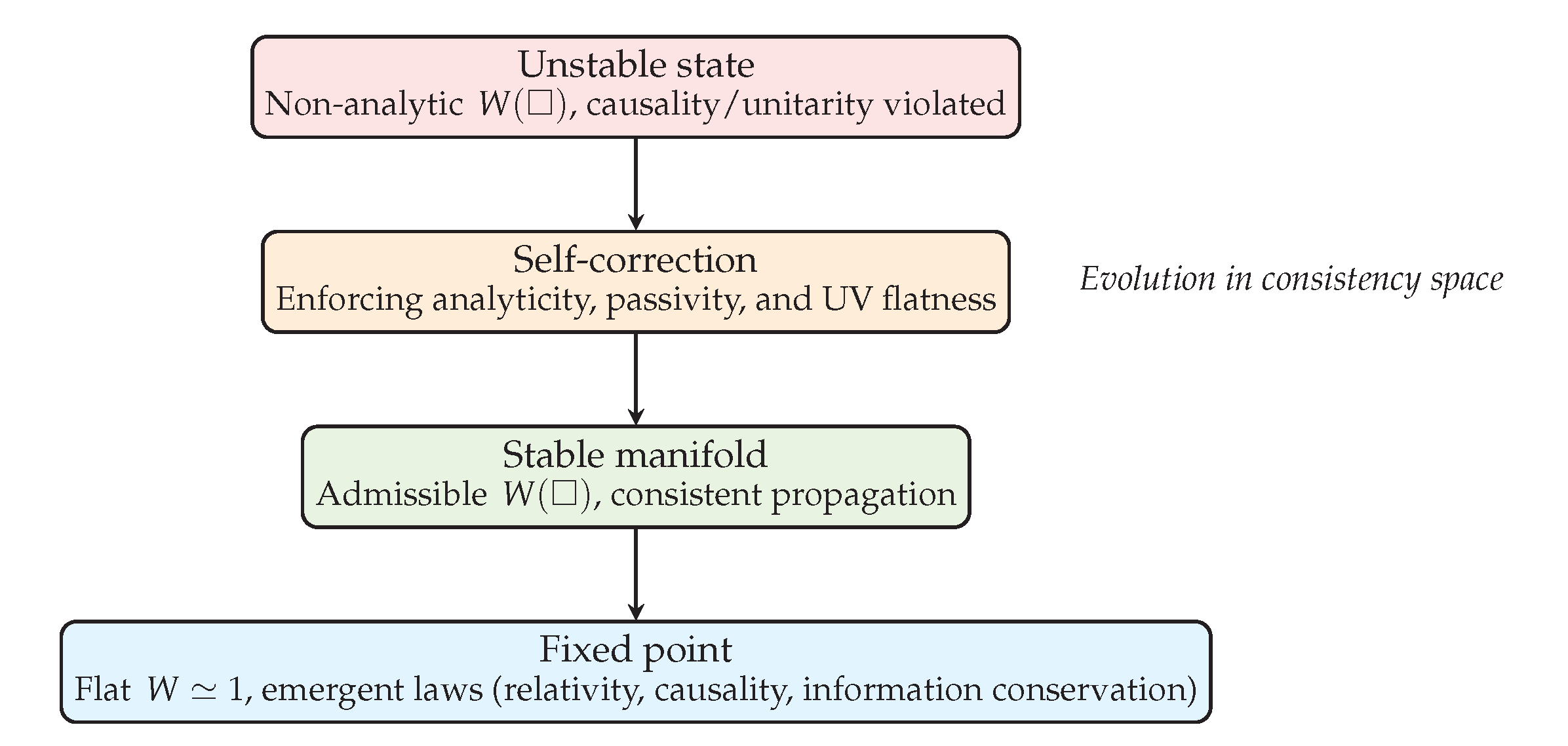
In summary, the vacuum does not obey the laws of physics; it is the dynamic system whose self-stabilization produces them. The constancy of c, the existence of causal propagation, and the preservation of information are the observable footprints of this deeper emergent equilibrium.
Appendix J. *
Concluding Reflection
To close, we briefly reflect on the conceptual implications of the framework.
In summary, the vacuum obeys the laws of physics precisely because these laws arise from its own dynamic self-stabilization. What we observe as the constancy of c, causal propagation, and the preservation of information are the visible traces of this emergent equilibrium.
Operationally, this equilibrium is tested through the band-invariant , under the conditions of analyticity, passivity, and UV flatness; thus the claim remains falsifiable while staying concept-first.
The laws we measure are the shadows of a deeper balance: the self-consistency by which existence sustains its own coherence. Light is the signature of consistency itself.
References
- M. Aspelmeyer, T. J. M. Aspelmeyer, T. J. Kippenberg, and F. Marquardt, “Cavity optomechanics,” Rev. Mod. Phys. 86, 1391–1452 (2014). [CrossRef]
- G. Bimonte, D. G. Bimonte, D. López, and R. S. Decca, “Isoelectronic determination of the thermal Casimir force,” Phys. Rev. B 93, 184434 (2016). [CrossRef]
- M. Bordag and I. Pirozhenko, “Casimir effect at nonzero temperature: recent developments,” Int. J. Mod. Phys. A 30, 1550014 (2015).
- M. Bordag, G. L. Klimchitskaya, U. Mohideen, and V. M. Mostepanenko, Advances in the Casimir Effect (Oxford Univ. Press, 2009). ISBN: 978-0199238743.
- S. M. Carr, S. I. S. M. Carr, S. I. Woods, T. M. Jung, A. C. Carter, and R. U. Datla, “Experimental measurements and noise analysis of a cryogenic radiometer,” Rev. Sci. Instrum. 85, 075105 (2014). [CrossRef]
- H. B. Callen and T. A. Welton, “Irreversibility and Generalized Noise,” Phys. Rev. 83, 34–40 (1951). [CrossRef]
- E. Calloni, L. E. Calloni, L. Di Fiore, G. Esposito, and L. Rosa, “Gravitational experiments in a quantum vacuum,” Phys. Rev. D 91, 102002 (2015). [CrossRef]
- H. B. G. Casimir, “On the attraction between two perfectly conducting plates,” Proc. K. Ned. Akad. Wet. 51, 793 (1948).
- C. S. Chang, S. G. C. S. Chang, S. G. Parker, and R. L. Byer, “Cryogenic optical resonators with 10-15 fractional frequency stability,” Rev. Sci. Instrum. 90, 065112 (2019).
- R. S. Decca, D. R. S. Decca, D. López, E. Fischbach, and D. E. Krause, “Measurement of the Casimir force between dissimilar metals,” Phys. Rev. Lett. 94, 240401 (2005). [CrossRef]
- D. J. Fixsen, “The Temperature of the Cosmic Microwave Background,” Astrophys. J. 707, 916–920 (2009). [CrossRef]
- J. D. Jackson, Classical Electrodynamics, 3rd ed. (Wiley, 1999).
- R. L. Jaffe, “The Casimir effect and the quantum vacuum,” Phys. Rev. D 72, 021301(R) (2005). [CrossRef]
- A. J. H. Kamminga, “Vacuum Density and Cosmic Expansion: A QEV Model,” Preprints (2025). [CrossRef]
- A. J. H. Kamminga, “Vacuum Energy with Natural Bounds: A Spectral Approach without Fine-Tuning,” Preprints (2025). [CrossRef]
- G. L. Klimchitskaya, U. G. L. Klimchitskaya, U. Mohideen, and V. M. Mostepanenko, “The Casimir force between real materials: Experiment and theory,” Rev. Mod. Phys. 81, 1827–1885 (2009). [CrossRef]
- R. Kubo, “Statistical-Mechanical Theory of Irreversible Processes,” J. Phys. Soc. Jpn. 12, 570 (1957). [CrossRef]
- R. Kubo, “The fluctuation-dissipation theorem,” Rep. Prog. Phys. 29, 255 (1966).
- L. D. Landau and E. M. Lifshitz, Electrodynamics of Continuous Media, 2nd ed. (Pergamon, Oxford, 1984).
- S. K. Lamoreaux, “Demonstration of the Casimir Force in the 0.6 to 6 μm Range,” Phys. Rev. Lett. 78, 5–8 (1997). [CrossRef]
- J. C. Mather, D. J. J. C. Mather, D. J. Fixsen, R. A. Shafer, C. Mosier, and D. T. Wilkinson, “Calibrator design for the COBE Far Infrared Absolute Spectrophotometer (FIRAS),” Astrophys. J. 512, 511–520 (1999). [CrossRef]
- K. A. Milton, The Casimir Effect: Physical Manifestations of Zero-Point Energy (World Scientific, 2001).
- K. A. Milton, “The Casimir effect: Recent controversies and progress,” J. Phys. A: Math. Gen. 37, R209–R277 (2004). [CrossRef]
- K. A. Milton, “Applications of the Casimir effect,” J. Phys. Conf. Ser. 161, 012001 (2011). [CrossRef]
- U. Mohideen and A. Roy, “Precision Measurement of the Casimir Force from 0.1 to 0.9 μm,” Phys. Rev. Lett. 81, 4549–4552 (1998). [CrossRef]
- V. M. Mostepanenko, “Status of modern Casimir force measurements and theoretical approaches,” Universe 7, 84 (2021). [CrossRef]
- B. A. Nosek et al., “Promoting an open research culture,” Science 348, 1422–1425 (2015).
- R. D. Peng, “Reproducible research in computational science,” Science 334, 1226–1227 (2011). [CrossRef]
- Planck Collaboration, “Planck 2018 results. I. Overview and the cosmological legacy of Planck,” Astron. Astrophys. 641, A1 (2020). [CrossRef]
- M. Rossi, D. M. Rossi, D. Mason, J. Chen, Y. Tsaturyan, and A. Schliesser, “Measurement-based quantum control of mechanical motion,” Nature 563(7729), 53–58 (2018). [CrossRef]
- S. G. Kaplan, S. I. S. G. Kaplan, S. I. Woods, E. L. Shirley, A. C. Carter, T. M. Jung, J. E. Proctor, D. R. Sears, and J. Zeng, “Design, calibration, and application of a cryogenic low-background infrared radiometer for spectral irradiance and radiance measurements from 4 to 20 μm wavelength,” Opt. Eng. 60(3), 034102 (2021). [CrossRef]
- A. Stange, M. A. Stange, M. Wagner, and F. M. de Leonardis, “Casimir force measurements in the deep submicron regime with optomechanical sensors,” Nat. Phys. 18, 271–276 (2022).
- R. Steiner, “The new definition of the kilogram,” Metrologia 54, A1–A10 (2017).
- V. Stodden, M. V. Stodden, M. McNutt, D. H. Bailey et al., “Enhancing reproducibility for computational methods,” Science 354, 1240–1241 (2016).
- D. V. Strekalov, N. D. V. Strekalov, N. Yu, and C. M. Savory, “High-Q millimetre-wave whispering-gallery-mode resonators for frequency metrology,” IEEE Trans. Ultrason. Ferroelectr. Freq. Control 68(7), 2130–2140 (2021).
- B. Taschuk and G. Wilson, “Good enough practices in scientific computing,” PLoS Comput. Biol. 13, e1005510 (2017). [CrossRef]
- M. Urban, F. M. Urban, F. Couchot, X. Sarazin, and A. Lambrecht, “The quantum vacuum as the origin of the speed of light,” Eur. Phys. J. D 67, 58 (2013).
Figure 1.
Operational pipeline: a single vacuum window and a calibrated, unit-area sensitivity combine into the platform-independent figure of merit . Normalization: (unit-area). Curves rescaled for visibility; schematic, not to scale.
Figure 1.
Operational pipeline: a single vacuum window and a calibrated, unit-area sensitivity combine into the platform-independent figure of merit . Normalization: (unit-area). Curves rescaled for visibility; schematic, not to scale.

Disclaimer/Publisher’s Note: The statements, opinions and data contained in all publications are solely those of the individual author(s) and contributor(s) and not of MDPI and/or the editor(s). MDPI and/or the editor(s) disclaim responsibility for any injury to people or property resulting from any ideas, methods, instructions or products referred to in the content. |
© 2025 by the authors. Licensee MDPI, Basel, Switzerland. This article is an open access article distributed under the terms and conditions of the Creative Commons Attribution (CC BY) license (http://creativecommons.org/licenses/by/4.0/).
Copyright: This open access article is published under a Creative Commons CC BY 4.0 license, which permit the free download, distribution, and reuse, provided that the author and preprint are cited in any reuse.


