
Submitted:
13 October 2025
Posted:
14 October 2025
You are already at the latest version
Abstract
Fundamental kinematic constraints in condensed matter systems, such as Lieb–Robinson bounds, sound velocities, and finite bandwidths, impose strict limits on quasiparticle group velocities. We show that these ubiquitous bounds naturally lead to an emergent minimal position uncertainty, derived entirely within standard quantum mechanics without deforming the canonical commutation relations. Using a variational Sturm–Liouville formulation in momentum space, we establish a universal relation that links spatial resolu- tion limits directly to measurable system parameters. Beyond variance-based measures, we further characterize this emergent scale using Shannon entropy, Fisher information, and quantum Fisher information, thereby revealing its information-theoretic fingerprint. Representative estimates for semiconduc- tors and ultracold atomic systems yield minimal lengths on the nanometer scale, many orders of magnitude above the Planck length but fundamental within effective descriptions. Our results provide a unified perspective that connects abstract localization limits with tangible condensed matter con- straints, opening new avenues for experimental and metrological exploration of minimal-length phenomena.
Keywords:
minimal length
; quantum information
; fisher information
; condensed matter systems
; Lieb–Robinson bounds
1. Introduction
The concept of a minimal length has long been regarded as a natural consequence of attempts to unify quantum mechanics with gravity. Early arguments, based on the interplay of the Heisenberg uncertainty principle and gravitational collapse, suggest that spatial resolution cannot be arbitrarily refined beyond the Planck scale [1,2]. More formal approaches, such as string theory [3,4] and loop quantum gravity [5,6], also predict the emergence of a minimal observable length. At the effective level, these insights are often encoded in generalized uncertainty principle (GUP) frameworks, which introduce modified commutation relations between position and momentum [7,8].
A parallel line of research has emphasized that minimal length features can also emerge from purely kinematic considerations, without altering the canonical algebra. Bosso et al. [9] recently demonstrated that imposing a cutoff in wave-number space suffices to induce a finite resolution limit in position, showing that minimal length can be reinterpreted as a Fourier-theoretic effect. This perspective opens the possibility that minimal uncertainties may arise in a much broader range of physical contexts, beyond quantum gravity.
Indeed, condensed matter systems naturally exhibit kinematic bounds that mimic the role of a momentum or velocity cutoff. The Lieb–Robinson bound imposes a maximum speed for the propagation of correlations in spin systems [10,11], while phonons and excitons propagate at finite sound velocities. Electronic quasiparticles in semiconductors are also constrained by finite Fermi velocities and limited bandwidths. In such systems, the effective mass approximation
is valid only within a bounded region of momentum space. This observation provides a natural arena where the emergence of minimal position uncertainty can be investigated operationally.
In this work, we show that a universal minimal position uncertainty arises directly from the existence of a maximal group velocity, without the need for deformed commutation relations or quantum-gravity specific mechanisms. Employing a variational Sturm–Liouville formulation in momentum space with Dirichlet boundary conditions at , we derive the fundamental result
This relation bridges abstract mathematical cutoffs with physically measurable bounds, and places minimal length in the context of effective theories of quasiparticles.
Beyond establishing the uncertainty relation itself, we complement the analysis with information-theoretic measures. Quantities such as the Shannon entropy, the Fisher information, and the quantum Fisher information (QFI) play a central role in modern quantum physics: they quantify localization and delocalization in conjugate variables [12], provide operational bounds via the Cramér–Rao inequality [13], and are deeply connected to entropic formulations of the uncertainty principle [14]. In addition, these measures have found wide applications in quantum information, statistical physics, and condensed matter, serving as tools to characterize correlations, coherence, and critical phenomena. Recent contributions have also demonstrated their relevance in effective models and foundational analyses [15,16]. In the present context, we compute these measures for the minimal-uncertainty state induced by the momentum cutoff, thereby clarifying how the restriction in momentum space modifies statistical distinguishability and entropic trade-offs. Remarkably, we find that the classical Fisher information associated with momentum measurements coincides exactly with the QFI for momentum displacements, demonstrating that the natural measurement basis saturates the quantum Cramér–Rao bound.
The paper is organized as follows. Sec. Section 2 develops the variational formulation in momentum space and derives the minimal position uncertainty. Sec. Section 3 presents the evaluation of Shannon entropy, Fisher information, and QFI, with comparisons to the Gaussian benchmark. Section 4 discusses applications to selected condensed matter systems, providing estimates of minimal lengths using realistic parameters. Section 5 contains a broader discussion of the implications, emphasizing the emergent and system-dependent nature of minimal length. Finally, Section 6 summarizes the main conclusions and outlines perspectives for future research.
2. Physical Motivation and Variational Formulation
2.1. Bounded Group Velocity in Effective Systems
A ubiquitous feature of condensed matter systems is the existence of finite propagation speeds. For instance, the Lieb–Robinson bound imposes a maximum speed for the spread of correlations in spin chains [10,11]; phonons and excitons propagate at the sound velocity in crystals; and electronic quasiparticles are limited by Fermi velocities and finite bandwidths in semiconductors. In all these cases, the effective mass approximation
is valid only within a restricted momentum window. This naturally introduces a maximal group velocity,
which in turn defines a bounded momentum domain,
Thus, even for a free quasiparticle, the effective description is inherently restricted in momentum space. This restriction plays the same mathematical role as the momentum cutoffs that appear in generalized uncertainty principle models, but here it arises directly from physical kinematics.
2.2. Variational Sturm–Liouville Formulation
Having established the physical origin of the cutoff, we now derive the corresponding minimal uncertainty in position. Consider a normalized momentum-space wavefunction defined on the finite interval . The position variance can be expressed as
Minimization of under the normalization constraint leads to the Sturm–Liouville eigenvalue problem
where is a Lagrange multiplier. The ground-state solution is the even function
which yields the minimal position uncertainty
This relation demonstrates that the existence of a maximal group velocity implies a fundamental resolution limit in position space, emergent within the standard formalism of quantum mechanics.
The choice of Dirichlet boundary conditions,
is not arbitrary but reflects the physical meaning of the cutoff in momentum space. In the effective description, momenta outside the domain are not physically accessible, as group velocities are bounded by . Requiring that the wavefunction vanish at the endpoints therefore encodes the impossibility of occupying states exactly at or beyond the cutoff. This ensures that the Hilbert space is restricted to square-integrable functions strictly confined to the admissible region. Moreover, Dirichlet conditions are mathematically natural for Sturm–Liouville problems on finite intervals, as they guarantee a discrete spectrum and orthogonal eigenfunctions. Alternative boundary conditions, such as Neumann or periodic, would either lack a clear physical interpretation in this context or would not enforce strict confinement at the cutoff. Thus, Dirichlet boundary conditions are both physically motivated and mathematically consistent.
In Figure 1 we illustrate the qualitative difference between an unbounded Gaussian state and the minimal-uncertainty state obtained under a finite momentum cutoff. In momentum space, the Gaussian extends over the whole axis, while the cosine solution is strictly confined to the interval . The Fourier duality enforces that this confinement leads to a broader spatial profile in position space, where the cutoff-induced state exhibits a finite minimal width. This visualization captures the essence of our result: restricting quasiparticle dynamics to a bounded group velocity domain inevitably produces an emergent resolution limit in real space.
Figure 2 depicts the variation of the minimal position uncertainty as a function of the effective mass and the maximal velocity , governed by the universal relation . The plot reveals that the minimum spatial resolution decreases as the effective mass or maximal velocity increases, highlighting the inverse proportionality of these parameters with respect to . To accommodate the wide range of magnitudes, all axes are presented on a logarithmic scale. It is observed that systems with lighter quasiparticles and lower propagation velocities exhibit significantly larger minimal lengths, whereas higher masses and velocities shift the scale toward nanometric or smaller values, consistent with the predictions for real systems discussed in the text.
The variational analysis establishes that the existence of a maximal group velocity enforces a minimal position uncertainty, realized by the cosine state of Eq. (8). While this result already captures the core geometric limitation imposed by the cutoff in momentum space, it is instructive to complement the picture with a broader set of information-theoretic measures. Indeed, quantities such as the Shannon entropy, the Fisher information, and the quantum Fisher information provide independent perspectives on localization, delocalization, and statistical distinguishability. By evaluating these measures for the cosine state we can characterize not only its variance but also its entropic properties and metrological performance, thereby gaining a deeper understanding of how the momentum cutoff reshapes the information content of quasiparticle states.
3. Information-Theoretic Measures
In this section1 we characterize the minimal-uncertainty state,
using three central information-theoretic quantities: the Shannon entropy, the Fisher information, and the quantum Fisher information. These measures provide complementary perspectives on localization, delocalization, and statistical distinguishability, thereby going beyond the variance-based analysis of Sec. Section 2. In addition, an initial exploration of further informational descriptors, namely the Rényi and Tsallis entropies, is presented in Appendix C, offering a broader picture of how the momentum cutoff reshapes the informational structure of the state.
3.1. Shannon Entropy in Momentum Space
The differential Shannon entropy is defined as
Using the normalization integral
and performing the change of variable , the integral can be evaluated in closed form. The result is
In terms of the emergent minimal length,
this expression becomes
As usual for differential entropy, the absolute value depends on the unit of p; nevertheless, the comparison with other distributions is meaningful when the same unit is adopted.
3.2. Fisher Information in Momentum Space
The Fisher information associated with translations in p is
A direct calculation yields
Figure 3 displays the behavior of the Shannon entropy (left) and the Fisher information (right) for the state that minimizes the position uncertainty under a finite momentum cutoff. For finite values of , the Shannon entropy remains bounded, reflecting the restricted support in momentum space, while the Fisher information grows with , consistently with the inverse scaling of the minimal position uncertainty . In the standard case, obtained in the limit , the momentum distribution spreads without bound: the Shannon entropy diverges to and the Fisher information vanishes, recovering the usual quantum–mechanical scenario where no fundamental minimal length exists. The figure therefore illustrates how the introduction of a finite cutoff qualitatively reshapes the informational balance, enforcing a finite resolution scale absent in the unconstrained case.
3.3. Comparison with the Gaussian Case
For reference, consider the Gaussian momentum distribution with variance ,
For this case the entropy and Fisher information are well known:
The variance of the cosine state (11) can be evaluated exactly:
Choosing a Gaussian with , one obtains slightly larger entropy and smaller Fisher information compared to the cosine state. For (with for convenience):
Thus the truncated cosine exhibits lower entropy and higher Fisher information than the Gaussian with the same variance.
3.4. Entropic Uncertainty Relation
The analysis of the Shannon entropy in position space poses additional challenges compared to the momentum-space case. While admits a closed analytic expression, the Fourier transform of the truncated cosine state involves oscillatory integrals that do not lead to a compact closed form for . As a result, the evaluation of
cannot be carried out analytically in a straightforward way. These difficulties, which are discussed in detail in Appendix B, motivate the adoption of a numerical approach. In what follows, we compute numerically from the Fourier transform of Eq. (8), ensuring consistency with normalization and convergence tests. This procedure allows us to quantify the position-space entropy and to compare it directly with the momentum-space result.
The position-space entropy can be evaluated numerically from the Fourier transform of Eq. (11). For and , we find , giving
This is consistent with the Białynicki–Birula–Mycielski (BBM) entropic uncertainty relation
which in natural units () gives the bound . The Gaussian state saturates this inequality, while the cosine state lies slightly above it, as expected from its non-Gaussian shape.
These results show that the information-theoretic properties of the cosine state are distinct from the Gaussian benchmark: the truncation in momentum space reduces the Shannon entropy and enhances the Fisher information. This dual behavior underscores the fact that the emergent minimal length is naturally associated with information-theoretic constraints as well as with uncertainty relations in the standard quantum framework.
3.5. Quantum Fisher Information for Translations
We consider the quantum Fisher information (QFI) associated with two natural estimation tasks for the quasiparticle state (11): (i) estimation of a small position translation a, generated by the momentum operator ; (ii) estimation of a small momentum translation b, generated by the position operator . For a pure state undergoing a unitary family generated by , the QFI is given by
3.5.1. QFI for Position Translations (Parameter a)
A translation in position by a is generated by , so the QFI for estimating a is
Using the momentum-space representation the variance of is just the variance of the probability density . For the cosine state
one obtains the closed form variance (computed explicitly)
Hence
Expressing this QFI in terms of the emergent minimal length gives the compact form
Numerical example: for and one finds and hence .
3.5.2. QFI for Momentum Translations (Parameter b)
A translation in momentum by b is generated by , so the QFI for estimating b is
For the cosine state the position variance is precisely the quantity we minimized in the variational formulation; the minimal position variance equals . Therefore
Using this is algebraically identical to
3.5.3. Relation with the Classical Fisher Information in p
Recall the classical Fisher information we computed in momentum space,
see Eq. (18). Comparing with Eq. (35) we observe the exact identity
This equality has a transparent interpretation: is the classical Fisher information associated with estimating a momentum displacement b when measuring in the momentum basis. For the present pure state the momentum-basis measurement is optimal for estimating b, hence the classical Fisher equals the QFI for b. In other words, the momentum measurement saturates the quantum Cramér–Rao bound for this parameter.
By contrast, the QFI for position translations (Eq. (31)) is a different quantity and scales as (or ), as expected from dimensional analysis.
3.5.4. Remarks and Interpretation
The quantum Fisher information for momentum translations, , is directly governed by the minimal position width : a smaller minimal width leads to a larger QFI for estimating momentum shifts. This agrees with the intuition that states more localized in position are more sensitive to displacements in momentum.
A central point of our analysis is the exact equality
which shows that the quantum Fisher information coincides with the classical Fisher information computed from the momentum probability distribution. This identity highlights that a projective measurement in the momentum basis is already optimal for extracting information about momentum displacements in the cosine state. In other words, no more elaborate measurement strategy can outperform the simple momentum measurement.
This result establishes a direct bridge between the quantum and classical information-theoretic descriptions: the operational content of the quantum Fisher information is fully realized by the classical Fisher information associated with the chosen measurement. The fact that both coincide underscores the consistency of the information-theoretic framework and gives a clear physical interpretation of the role of the minimal width in momentum estimation. Importantly, this coincidence is not generic, but a distinctive feature of the cosine minimal state, which provides an illuminating example of the tight connection between quantum estimation and classical statistical information.
The comparison in Table 1 highlights the information-theoretic fingerprint of the emergent minimal length. First, the cosine state has a smaller momentum entropy than the Gaussian benchmark with the same variance, since the support is bounded and the distribution is more localized in p. This comes at the cost of a larger position entropy , reflecting the delocalization of the state in x-space. Consequently, the entropy sum lies strictly above the Białynicki–Birula–Mycielski bound, whereas the Gaussian saturates it; the cutoff therefore prevents the realization of minimal entropic uncertainty. In terms of Fisher information, the cosine state is more sensitive to infinitesimal momentum shifts than the Gaussian, a direct manifestation of its oscillatory structure in p-space. Remarkably, the quantum Fisher information for momentum displacements coincides exactly with the classical Fisher information, showing that the natural momentum basis already achieves the optimal precision allowed by quantum mechanics. Taken together, these results reveal that the momentum cutoff not only enforces a minimal position uncertainty, but also modifies the balance between entropic trade-offs and metrological performance. This dual effect is absent in Gaussian states, and constitutes a distinctive signature of the emergent minimal length.
4. Applications: Minimal Lengths in Real Systems
Equation (9) shows that any finite bound on the group velocity implies a corresponding minimal position uncertainty. Since both and can be extracted from experimental data or theoretical models, Eq. (9) provides a direct and operational method to estimate localization limits in real condensed matter systems.
4.1. Methodology
For electrons in semiconductors, we adopt effective masses from standard band structure parameters, and take as of the order of the Fermi velocity. For excitons, the group velocity is bounded by the sound velocity of the host crystal. For ultracold atoms, is determined by measured propagation speeds of correlations in optical lattices.
4.2. Representative Estimates
The estimates in Table 2 indicate that lies in the nanometric to sub-micrometric range, many orders of magnitude above the Planck length yet fundamental within effective theories. In semiconductors, this bound constrains the spatial resolution of electron and exciton localization, while in ultracold gases it limits correlation measurements and quantum state tomography. Figure 4 illustrates these results across representative condensed matter and atomic platforms: despite variations in effective mass and characteristic velocities, the minimal lengths consistently remain in the same regime. This shows that is neither abstract nor negligible, but an operational constraint whose precise value depends on the quasiparticle considered, in contrast to the universal Planckian bound of quantum gravity.
5. Discussion: Limitations, Originality and Implications
The framework developed here should be regarded as an effective, system-dependent description. The quasiparticle dispersion , when restricted to a finite momentum domain , is not a modification of the canonical structure of quantum mechanics, but an operational restriction reflecting the limited validity of the effective mass approximation. Near the cutoff scale, deviations from the parabolic band become relevant and the model ceases to be quantitatively reliable. Nevertheless, the analysis demonstrates that the mere existence of a maximal group velocity already implies a finite minimal position uncertainty, without invoking deformed commutation relations or modified relativity principles.
It is important to emphasize the originality of this perspective. Previous works, such as Bosso et al., introduced cutoffs in wave-number space as abstract kinematical assumptions. In contrast, the cutoff considered here has a direct physical origin: it is determined by the maximum attainable velocity in condensed matter systems, whether set by Lieb–Robinson bounds, sound velocities, or finite bandwidths. This interpretation transforms what was previously a formal cutoff into a measurable, system-specific parameter. In this sense, the minimal length emerges not as a universal constant but as a relational feature of effective descriptions.
The analysis of information-theoretic measures in Sec. Section 3 further clarifies the physical significance of the emergent minimal length. The truncated cosine state, which minimizes the position variance, exhibits reduced momentum entropy and enhanced Fisher information relative to a Gaussian benchmark. This means that the cutoff not only enforces a bound on spatial resolution but also reshapes the informational balance between conjugate domains. The fact that shows that momentum-space measurements remain optimal for parameter estimation, while the non-saturation of the entropic uncertainty relation indicates that the cutoff introduces irreducible informational costs. Thus, minimal length here is not merely a geometric constraint, but a limit on the informational and metrological resources available in effective theories.
These results suggest several implications. For theory, they offer an algebra-preserving, information-theoretically enriched alternative to generalized uncertainty principle models. For experiments, they point to operational limits in quantum tomography, wavepacket engineering, and state reconstruction in semiconductors, excitonic systems, and ultracold gases. For foundations, they illustrate how concepts often associated with quantum gravity can naturally emerge in condensed matter contexts as system-dependent constraints, providing a unifying perspective across disparate energy scales. In this sense, the present framework highlights that minimal lengths should be understood not only as fundamental constants, but also as emergent features reflecting the kinematics and informational structure of effective systems.
Figure 5 provides a schematic comparison between three different scenarios concerning minimal length. In standard quantum mechanics, no momentum cutoff is present and the position uncertainty can, in principle, be reduced without bound. In condensed matter systems, however, the existence of a maximal group velocity imposes an effective cutoff in momentum space, leading to an emergent minimal length that is relational and system-dependent. By contrast, in quantum gravity approaches the cutoff is interpreted as fundamental, typically linked to the Planck scale, and thus defines a universal minimal length. This comparison highlights the distinct conceptual status of the minimal uncertainty obtained in our framework.
6. Conclusion
We have shown that the existence of a maximal group velocity, a generic feature of condensed matter systems, implies an emergent minimal uncertainty in position. By restricting the momentum domain to and applying a variational Sturm-Liouville formulation, we derived the universal relation
which connects a kinematic constraint with a fundamental resolution bound. This minimal length emerges without altering the canonical axioms of quantum mechanics.
Our approach translates an abstract cutoff into a physically measurable parameter: the maximal velocity of quasiparticles. This makes the concept of minimal length operational and system-dependent, bridging mathematical formulations with condensed matter phenomenology.
Our analysis of information-theoretic quantities—Shannon entropy, Fisher information, and quantum Fisher information (QFI)—reveals that the cutoff not only imposes a geometric limit but also profoundly reshapes the informational and metrological structure of the effective theory. We showed that the minimal-uncertainty (cosine) state exhibits reduced Shannon entropy in momentum space and enhanced Fisher information, compared to a Gaussian state of the same variance. Furthermore, the quantum Fisher information for momentum translations () was found to coincide exactly with the classical Fisher information , demonstrating that measurements in the momentum basis are optimal for estimating momentum shifts, saturating the quantum Cramér-Rao bound. The entropic uncertainty relation of Bialynicki-Birula-Mycielski is not saturated, indicating an irreducible informational cost associated with the cutoff.
These results highlight that emergent minimal lengths act simultaneously as geometric and informational constraints, modifying the balance between entropy, statistical distinguishability, and metrological sensitivity—a duality absent in Gaussian states that constitutes a distinctive signature of the minimal uncertainty induced by a bounded velocity.
Some avenues for future research arise naturally. On the theoretical side, one may explore variational principles for states that maximize Shannon entropy or Fisher information under the same cutoff, providing a broader taxonomy of information-extremal states in effective models (see Appendix A). On the experimental side, quantitative estimates of in semiconductors, excitons, and ultracold atoms could be probed through wavepacket dynamics and quantum state tomography. Finally, at the conceptual level, our framework suggests that ideas usually associated with quantum gravity—such as minimal lengths—can appear naturally in low-energy systems as emergent, relational constraints, thus offering a unifying perspective across scales and contexts.
Appendix A. Variational Principles for Shannon Entropy and Fisher Information
All variational problems considered here are posed on the finite momentum interval and must respect the physical boundary condition
i.e. the momentum-space wavefunction vanishes at the endpoints.
Appendix A.1. Maximization of the Shannon Entropy
The differential Shannon entropy in momentum space is
subject to normalization
and Dirichlet boundary conditions (A1).
To derive stationary conditions we vary with respect to the real-valued amplitude (variations are required to vanish at the endpoints because of the Dirichlet constraint). Writing and performing an infinitesimal variation with , we obtain (step-by-step)
while the variation of the normalization constraint gives
Introducing a Lagrange multiplier and imposing stationarity yields
for all admissible . Hence the Euler–Lagrange condition in the interior is
i.e. the stationary solution must be constant in the interior. However, a constant nonzero amplitude cannot satisfy the Dirichlet boundary conditions . Therefore there is no smooth interior function that simultaneously satisfies the Euler–Lagrange equation and the Dirichlet BCs: the maximum is not attained in the admissible set as a classical interior solution.
The correct statement is that the supremum of under the support and Dirichlet constraints is approached by sequences of functions that are essentially uniform in the interior and decay smoothly to zero in boundary layers near . In the limit where these boundary layers become arbitrarily narrow the entropy approaches that of the uniform distribution on the interval,
but no admissible function satisfying attains this value exactly. In practice, for physical and numerical work one therefore uses smooth approximants to the uniform profile (constant in the bulk, smoothed to zero near the endpoints), which achieve Shannon entropies arbitrarily close to (A5) while respecting Dirichlet BCs.
Appendix A.2. Variational Formulation for Fisher Information and Regularization
The Fisher information can be written (for real ) as
subject to and . The naive maximization problem is ill-posed: one can produce sequences of normalized functions with arbitrarily large gradient norm (for instance, by oscillating faster and faster in the interior while keeping Dirichlet zeros at the endpoints), hence . Thus, as anticipated, Fisher information requires an additional constraint to be physically meaningful.
A mathematically and physically transparent resolution is to introduce a regularization that penalizes excessive curvature. One convenient choice is the Tikhonov-type functional.
with regularization parameter . We enforce Dirichlet BCs and require that admissible belong to a Sobolev space ensuring existence of (e.g. with the trace ). Variation of yields (integration by parts, assuming ):
With Dirichlet BCs the terms proportional to at the endpoints vanish; however, boundary terms involving remain unless additional boundary conditions are imposed. Requiring natural boundary conditions (obtained from the vanishing of the full boundary contribution) leads to
so that the variation is well defined. Consequently, the Euler–Lagrange equation is the fourth-order linear eigenvalue problem.
with . Under these boundary conditions the problem has a discrete spectrum and a principal eigenfunction that provides the regularized maximizer of the Fisher functional for the chosen .
An alternative physically motivated choice is to impose clamped boundary conditions
which also kills all boundary terms and yields a well-posed eigenproblem. The choice between (A9) and (A11) should be guided by the physical regularity constraints of the specific system (e.g. smoothness enforced by finite microscopic bandwidth or experimental limitations).
Appendix A.2.1. Practical Remarks
For the Shannon problem, in practice one employs smooth approximations to the uniform interior profile that also satisfy the Dirichlet boundary conditions. Such approximants achieve entropies arbitrarily close to while remaining admissible functions. In the case of the Fisher problem, the appropriate strategy is to solve the regularized fourth-order eigenproblem (A10) (or its discretized version) for a physically chosen value of . The principal eigenfunction obtained in this way maximizes the penalized Fisher functional, and varying explores the trade-off between sensitivity and smoothness. From a numerical perspective, the discretization can be implemented with spectral (e.g. Chebyshev) or finite-element bases that enforce , providing stable solutions for moderate values of .
Appendix B. Analytic Representation and Scaling of the Position-Space Shannon Entropy
Starting from the momentum-space minimizer
its position-space wavefunction is the Fourier transform
Carrying out the elementary integration (using and ) one obtains the closed-form representation
Equivalently, introducing the dimensionless variable
and the (dimensionless) compact function
one has the exact scaling relation between the position densities:
The differential Shannon entropy in position can therefore be written as
Thus the position entropy separates into a universal dimensionless constant (the entropy of the profile ) and a simple logarithmic scaling with the momentum cutoff .
Define the universal constant
which depends only on the shape of the dimensionless function given in Eq. (A16). Then
Although admits the elementary representation (A16), the integral (A18) for does not reduce to a simple closed form in elementary constants. It is, however, a single convergent one-dimensional integral and can be evaluated numerically to arbitrary precision. Evaluating numerically one finds (for the branch of in Eq. (A16))
Hence, for general and ℏ,
Using the relation with the minimal length one can also express in terms of :
It is worth emphasizing some observations regarding the result above. The decomposition in Eq. (A19) is exact and entirely analytical, with the only non-elementary contribution being the constant , which encodes the entropy of the fixed, dimensionless profile . Once this constant is known, either numerically or to the desired level of precision, all values of follow directly from the logarithmic scaling with . The fact that does not admit a closed-form expression in terms of elementary constants is not unexpected, since the Shannon entropy of non-Gaussian Fourier pairs typically resists simplification. Nevertheless, the universality of makes it a useful reference constant, valid for the entire class of states generated by scaling and ℏ. From a practical perspective, can be computed reliably by numerical quadrature of the integrand over a sufficiently extended domain, or equivalently by FFT-based methods once is sampled; in both cases convergence is rapid due to the decay of the probability density at large .
Appendix C. Rényi and Tsallis Entropies for the Minimal Position Uncertainty State
In this appendix we complement the analysis of the main text by examining two additional entropic measures for the minimal position uncertainty state in momentum space, namely the Rényi and Tsallis entropies. These measures generalize the Shannon entropy in distinct directions and provide further insights into the informational properties of the cutoff-induced wavefunction.
The momentum distribution of the state,
leads to the family of integrals
which serve as the building blocks for both Rényi and Tsallis entropies.
Appendix C.1. Rényi Entropy
The Rényi entropy of order is defined as
For , Eq. (A25) recovers the Shannon entropy. The Rényi family therefore provides a continuous interpolation between different regimes of sensitivity to the probability distribution.
Physically, the Rényi entropy emphasizes different structural features of the minimal uncertainty state depending on the order . When , the entropy places greater weight on the high-probability regions of the distribution. In the present case, this highlights the oscillatory peaks near the center of the momentum domain, which dominate the structure of the cutoff-induced state. Conversely, when , the entropy becomes more sensitive to the low-probability regions, drawing attention to the suppressed tails near . In this way, the Rényi entropy allows one to dissect how the sharp momentum cutoff redistributes information between central and peripheral regions of the distribution. Such an analysis goes beyond the Shannon picture, where only the average spread is captured, and makes explicit the fact that the cutoff enforces a form of concentration in phase space that is not uniform across the support.
Appendix C.2. Tsallis Entropy
The Tsallis entropy of order q is defined as
In the limit , Eq. (A26) reduces again to the Shannon entropy, confirming the consistency of the generalization.
The Tsallis entropy is particularly relevant in systems where non-extensive statistical behavior arises or where cutoffs constrain the available phase space. In the present context, the momentum support is finite and sharply bounded, making the Tsallis measure especially suited to capturing the informational implications of such truncation. For , the Tsallis entropy accentuates the dominance of the central lobes of the distribution, effectively penalizing the suppressed tails. For , on the other hand, the entropy assigns more relative weight to the boundary regions, emphasizing the fact that the distribution abruptly vanishes at . This sensitivity reflects the inherently non-Gaussian nature of the cutoff-induced state and provides an alternative quantification of how information is distributed across its support.
From a physical perspective, the Tsallis entropy underscores that the emergent minimal length is not only a constraint on variance-based measures of localization but also a structural modification of the underlying information content. By tuning the parameter q, one can probe different aspects of this modification, revealing how the cutoff enforces a compromise between concentration around the origin and suppression near the boundaries of momentum space. In this sense, the Tsallis entropy highlights the non-extensive character of information in bounded systems and provides a natural framework to contrast the cutoff-induced state with the Gaussian states that saturate the standard uncertainty relations.
Appendix C.3. Discussion
Together, the Rényi and Tsallis entropies enrich the information-theoretic characterization of the minimal position uncertainty state. The Rényi family shows explicitly how the sharp cutoff redistributes information between core and tail regions, while the Tsallis family emphasizes the non-extensive and non-Gaussian features introduced by the finite support in momentum. Both measures reveal facets of the state that remain hidden in the Shannon description alone, and they demonstrate that the emergent minimal length is accompanied by an informational fingerprint that manifests differently depending on which entropic lens is applied. These considerations strengthen the interpretation of the minimal uncertainty not merely as a geometric bound but as a transformation of the informational landscape of effective quantum states.
Appendix D. Numerical Protocol for the Values Reported in Secs. 3.3 and 3.4
This appendix documents the exact numerical protocol used to compute the quantities displayed in Sections 3.3 and 3.4. The purpose is to make the computations fully reproducible and to provide practical details (discretization, algorithms, parameter choices, convergence checks, and expected numerical accuracy).
Appendix D.1. Overview of the Task
We consider a momentum-space wavefunction of compact support, for , and zero otherwise. From this we compute:
- momentum-space probability density , its variance , Shannon entropy and Fisher information ;
- the position-space wavefunction obtained by Fourier transform, the position probability density , and its Shannon entropy ;
- sums and comparisons with a Gaussian benchmark constructed with the same momentum variance.
All numerical results reported in the main text were obtained with the following protocol.
Appendix D.2. Software and Numerical Precision
- Implementation: Python 3.x using numpy and scipy (or equivalent).
- Floating point: IEEE double precision (64-bit). Use default numpy.float64.
- Reproducibility: no pseudorandom numbers are required. Save script and parameters with the manuscript.
- Recommended versions (example): numpy>=1.18, scipy>=1.4, matplotlib>=3.0.
Appendix D.3. Momentum-Space Setup and Normalization
Set units so that and choose for numerical experiments quoted in the main text. The momentum-space wavefunction is
This is normalized analytically: .
Appendix D.4. Discretization in Momentum Space
- Choose an even number of grid points. Typical values used: .
- Define a uniform grid on :with .
- Evaluate and on this grid.
- Numerical integrals over p are computed with the composite Simpson rule when high accuracy is desired (use scipy.integrate.simps) or with the trapezoidal rule for consistency checks. The grid above is uniform, so Simpson/trapezoid are straightforward and accurate.
Appendix D.5. Computation of Momentum-Space Quantities
Appendix D.10.10.1. Variance
computed with Simpson’s rule. Numerical convergence is tested by doubling and checking that changes by less than relative.
Appendix D.10.10.2. Shannon Entropy in p
The continuous Shannon entropy is approximated by
Care must be taken at grid points where is extremely small: in our case f is bounded away from zero inside , so direct evaluation is safe. Again use Simpson rule for the sum.
Appendix D.10.10.3. Fisher Information in p
We compute
Numerical procedure:
- (1)
- Compute using a high-order finite-difference formula (central difference of order 2 or 4). For stability, we used a 4th-order central difference:
- (2)
- Form pointwise the integrand and integrate with Simpson’s rule.
- (3)
- To avoid division by very small outside support, restrict integration to .
Convergence: vary and finite-difference stencil to confirm stability of to relative changes .
Appendix D.6. Computation of Position-Space Wavefunction via FFT
Appendix D.11.11.4. Fourier Transform Conventions
We use the unitary convention compatible with :
Numerically we want to compute at a discrete grid of x values using an FFT.
Appendix D.11.11.5. Zero Padding and Extended Momentum Grid
- To use FFT efficiently and avoid aliasing, embed the momentum samples into a periodic array of length (choose a power of two, e.g. or ).
- Create an array of length where entries corresponding to are , and the remaining entries are zero (zero-padding). This defines a periodic extension with period in x-space.
- The effective x-space grid resulting from the FFT is
- Choose large enough such that the x-domain contains the probability mass of with negligible truncation error. Typical choice used: , which gives a fine .
Appendix D.11.11.6. FFT Computation
- (1)
- Multiply the momentum array by the appropriate phase factor if needed to account for grid centering (use numpy.fft.fftshift/ifftshift as convenient).
- (2)
- Compute the inverse FFT (IFFT) and scale by the factor to approximate the continuous integral.
- (3)
- The resulting array approximates on the discrete grid.
- (4)
- Normalize numerically and check (relative error ).
Appendix D.7. Position-Space Shannon Entropy
Once is obtained and normalized, compute
Practical notes:
- The tails of are approximated over a finite domain. Ensure domain large enough (by adjusting and ) so that probability outside the domain is .
- To avoid numerical noise where is extremely small, impose a lower cutoff (e.g. values below treated as zero), but verify that choices do not affect within the desired tolerance.
- Check convergence by doubling and confirming changes by less than .
Appendix D.8. Gaussian Benchmark Construction
To compare with a Gaussian having the same variance :
Compute analytic expressions:
For position-space Gaussian with variance under the chosen Fourier convention, use the corresponding analytic Shannon entropy.
Appendix D.9. Convergence Tests and Error Estimates
We recommend the following checks to ensure numerical reliability:
- (1)
- Grid refinement: double and and verify that all reported quantities change by less than a target tolerance (e.g. relative).
- (2)
- Integration rule consistency: compare Simpson and trapezoidal integration for a subset of integrals.
- (3)
- Finite-difference stencil: vary derivative order for and check stability of .
- (4)
- Domain size: verify that increasing the effective x-domain (via larger or smaller ) does not alter beyond tolerance.
- (5)
- Normalization checks: ensure and numerically within machine precision.
Typical numerical accuracy achieved with the parameters above and double precision:
- : relative error .
- , : relative error (dominated by finite-difference approximation for derivatives).
- : absolute error to depending on grid.
Appendix D.10. Suggested Reproducible Script Outline (Summary)
- (1)
- Set constants: , . Choose , .
- (2)
- Build momentum grid and evaluate , .
- (3)
- Compute , via Simpson rule.
- (4)
- Compute with a 4th-order central difference and evaluate .
- (5)
- Zero-pad momentum array to length , apply shifts, compute IFFT to obtain , normalize and compute .
- (6)
- Run convergence tests (double and ).
Appendix D.11. Final Remark
The numerical values quoted in Secs. 3.3 and 3.4 were obtained following the protocol above. The code used for these computations is available upon request and can be provided as a short Python script/Colab notebook that reproduces the figures and tables presented in the manuscript.
References
- C. A. Mead, Possible connection between gravitation and fundamental length, Physical Review 135 (3B) (1964) B849.
- L. J. Garay, Quantum gravity and minimum length, International Journal of Modern Physics A 10 (02) (1995) 145–165.
- D. J. Gross, P. F. D. J. Gross, P. F. Mende, String theory beyond the planck scale, Nuclear Physics B 303 (3) (1988) 407–454.
- D. Amati, M. D. Amati, M. Ciafaloni, G. Veneziano, Can spacetime be probed below the string size?, Physics Letters B 216 (1-2) (1989) 41–47.
- C. Rovelli, L. C. Rovelli, L. Smolin, Discreteness of area and volume in quantum gravity, Nuclear Physics B 442 (3) (1995) 593–619.
- A. Ashtekar, J. A. Ashtekar, J. Baez, A. Corichi, K. Krasnov, Quantum geometry and black hole entropy, Physical Review Letters 80 (5) (1998) 904.
- A. Kempf, G. A. Kempf, G. Mangano, R. B. Mann, Hilbert space representation of the minimal length uncertainty relation, Physical Review D 52 (2) (1995) 1108.
- A. F. Ali, S. A. F. Ali, S. Das, E. C. Vagenas, Discreteness of space from the generalized uncertainty principle, Phys. Lett. B 678 (2009) 497–499.
- P. Bosso, L. P. Bosso, L. Petruzziello, F. Wagner, Minimal length: A cut-off in disguise?, Physical Review D 107 (12) (2023) 126009.
- E. H. Lieb, D. W. E. H. Lieb, D. W. Robinson, The finite group velocity of quantum spin systems, Communications in Mathematical Physics 28 (1972) 251–257.
- M. B. Hastings, Solving gapped hamiltonians locally, Physical Review B—Condensed Matter and Materials Physics 73 (8) (2006) 085115.
- I. Białynicki-Birula, J. I. Białynicki-Birula, J. Mycielski, Uncertainty relations for information entropy in wave mechanics, Communications in Mathematical Physics 44 (2) (1975) 129–132.
- M. G. Paris, Quantum estimation for quantum technology, International Journal of Quantum Information 7 (supp01) (2009) 125–137.
- S. Wehner, A. S. Wehner, A. Winter, Entropic uncertainty relations—a survey, New Journal of Physics 12 (2) (2010) 025009.
- J. Nascimento, F. J. Nascimento, F. Ferreira, V. Aguiar, I. Guedes, R. N. Costa Filho, Information measures of a deformed harmonic oscillator in a static electric field, Physica A: Statistical Mechanics and its Applications 499 (2018) 250–257.
- F. A. Pinheiro Ferreira, Information-theoretic analysis of a mass-dependent minimal length quantum harmonic oscillator, International Journal of Theoretical Physics 64 (10) (2025) 254.
- S. M. Sze, K. K. S. M. Sze, K. K. Ng, Physics of Semiconductor Devices, 3rd Edition, Wiley, Hoboken, NJ, 2007.
- C. Kittel, Introduction to Solid State Physics, 8th Edition, Wiley, New York, 2005.
- M. Fox, Optical Properties of Solids, 2nd Edition, Oxford University Press, Oxford, 2010.
- H. Haug, S. W. H. Haug, S. W. Koch, Quantum Theory of the Optical and Electronic Properties of Semiconductors, 5th Edition, World Scientific, Singapore, 2009.
- I. Bloch, J. I. Bloch, J. Dalibard, W. Zwerger, Many-body physics with ultracold gases, Rev. Mod. Phys. 80 (3) (2008) 885–964.
- M. Cheneau, P. M. Cheneau, P. Barmettler, D. Poletti, M. Endres, P. Schauß, T. Fukuhara, C. Gross, I. Bloch, C. Kollath, S. Kuhr, Light-cone-like spreading of correlations in a quantum many-body system, Nature 481 (2012) 484–487.
| 1 | All numerical estimates quoted here follow the procedure described in Appendix D. |
Figure 1.
Comparison between a Gaussian wavefunction (free particle, infinite momentum support) and the cosine solution with finite momentum cutoff . Left: momentum space profiles . Right: corresponding position space densities , showing the broader spatial spread induced by the cutoff.
Figure 1.
Comparison between a Gaussian wavefunction (free particle, infinite momentum support) and the cosine solution with finite momentum cutoff . Left: momentum space profiles . Right: corresponding position space densities , showing the broader spatial spread induced by the cutoff.
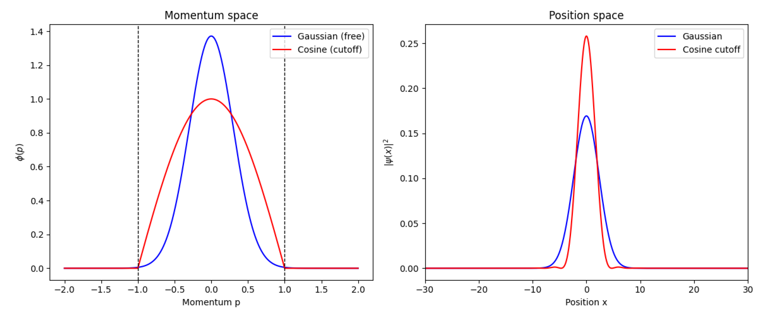
Figure 2.
Minimal uncertainty position as a function of the effective mass and the maximal group velocity , according to the universal relation . All axes are shown in logarithmic scale for better visualization. The plot highlights that lighter quasiparticles and lower propagation speeds yield larger minimal lengths, while heavier masses and higher velocities push towards the nanometric regime.
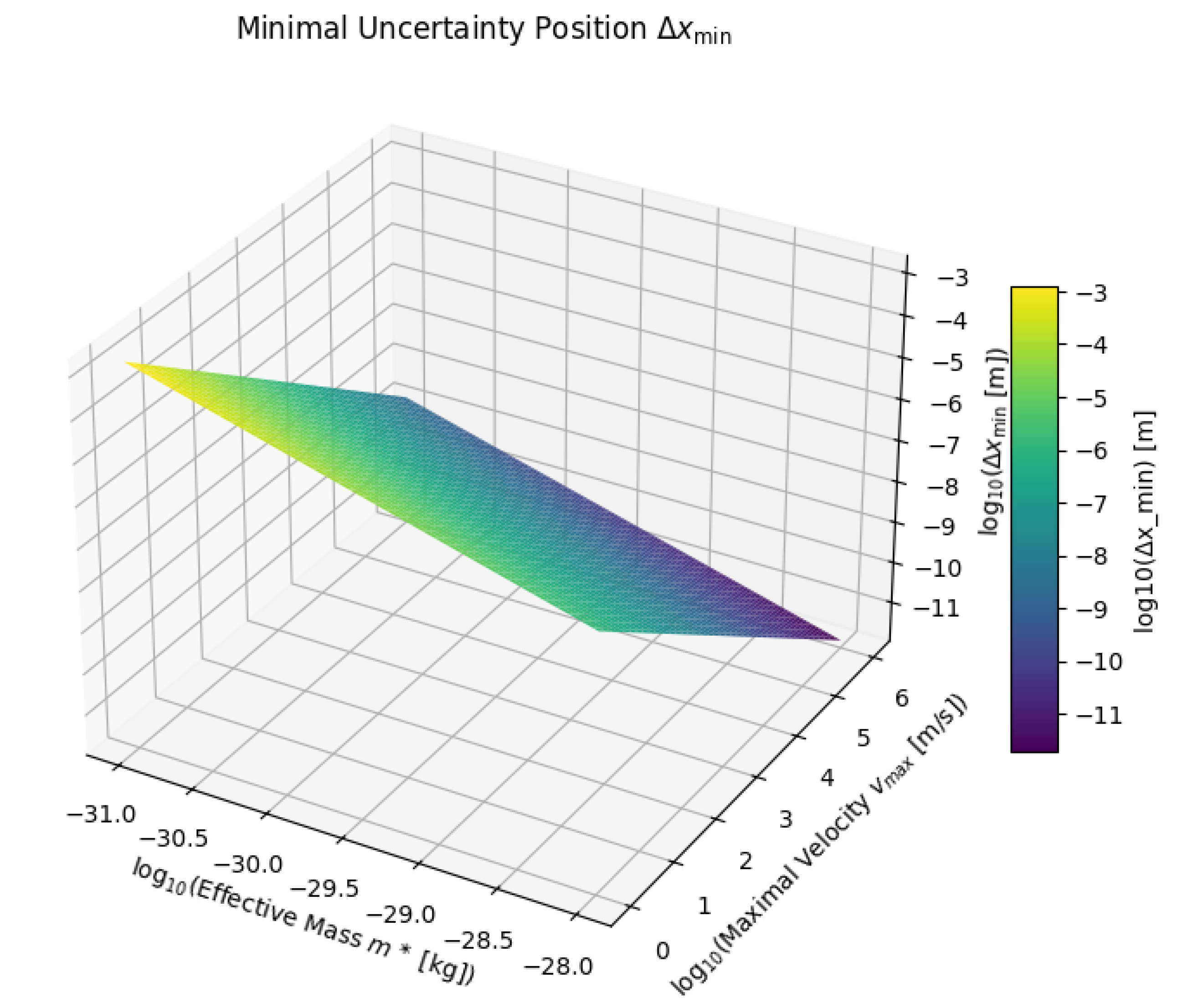
Figure 3.
Information-theoretic quantities of the minimal-uncertainty state: Shannon entropy (left) and Fisher information (right) as functions of the cutoff .
Figure 3.
Information-theoretic quantities of the minimal-uncertainty state: Shannon entropy (left) and Fisher information (right) as functions of the cutoff .
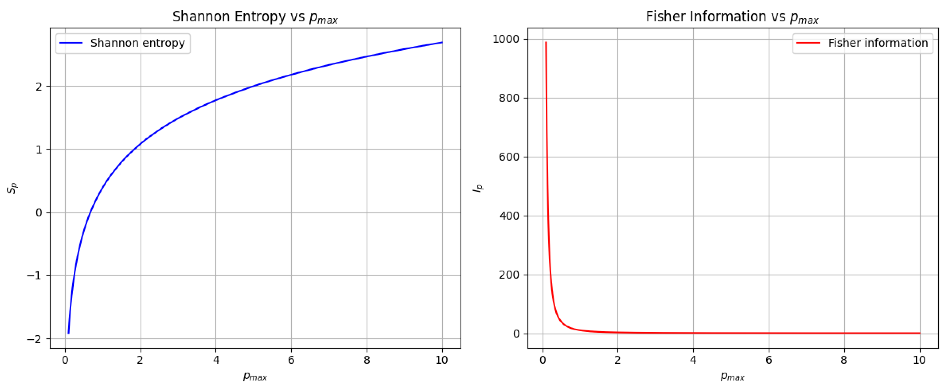
Figure 4.
Estimated minimal position uncertainty for different physical systems. The values are computed using Eq. 9 with the effective mass and maximal group velocity characteristic of each material or quasiparticle. The emergent minimal length is consistently nanometric, much larger than the Planck scale but fundamental to the effective description of each system.
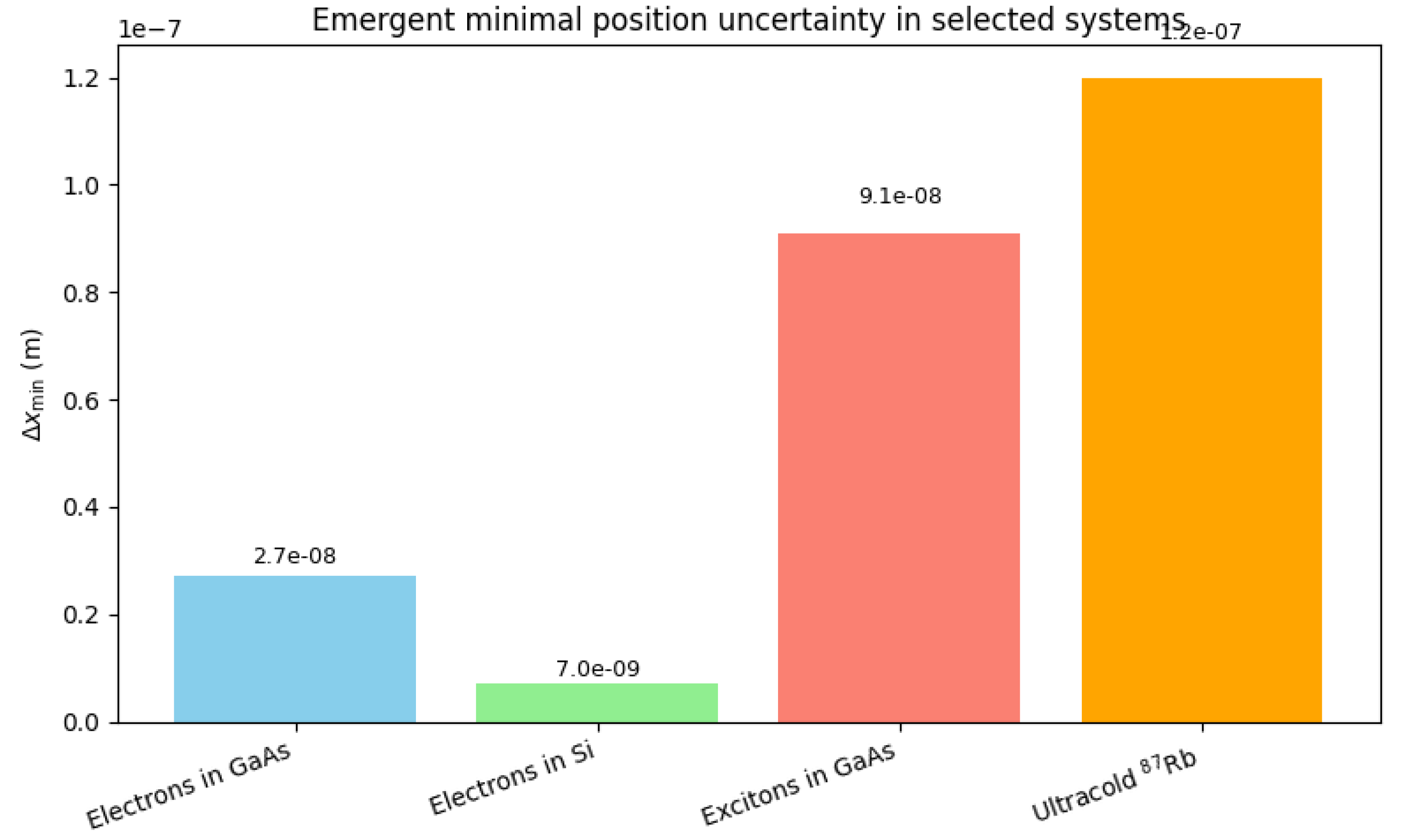
Figure 5.
Conceptual comparison of minimal length scenarios. In standard quantum mechanics (left) no cutoff exists and position uncertainty can be arbitrarily reduced. In condensed matter systems (center) a maximal group velocity enforces an emergent, system-dependent minimal length. In quantum gravity approaches (right) a fundamental cutoff appears, associated with the Planck length, leading to a universal minimal length.
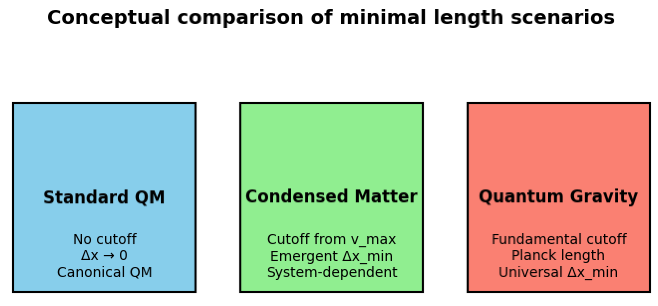

Table 1.
Comparison of information-theoretic quantities for the cosine minimal-uncertainty state and the Gaussian benchmark (same momentum variance). The cosine state corresponds to the truncated domain .
Table 1.
Comparison of information-theoretic quantities for the cosine minimal-uncertainty state and the Gaussian benchmark (same momentum variance). The cosine state corresponds to the truncated domain .
| Quantity | Cosine state | Gaussian state |
|---|---|---|
| Momentum Shannon entropy | Smaller (analytic, Eq. (14)) | Larger |
| Position Shannon entropy | Larger (numerical) | Smaller |
| Entropy sum | (not saturated) | (saturated) |
| Fisher information | Enhanced | Minimal (for given ) |
| Quantum Fisher information | (saturates bound) | |
| Interpretation | Sensitive to momentum shifts; broader in x | Optimal balance (Fourier duality) |
Table 2.
Representative estimates of the emergent minimal position uncertainty from Eq. (9) for selected systems. Effective masses are expressed relative to the free electron mass kg.
Table 2.
Representative estimates of the emergent minimal position uncertainty from Eq. (9) for selected systems. Effective masses are expressed relative to the free electron mass kg.
| System | (m/s) | (m) | Reference | |
|---|---|---|---|---|
| Electrons in GaAs | 0.067 | [17,18] | ||
| Electrons in Si | 0.26 | [17,18] | ||
| Excitons in GaAs | 0.05 | [19,20] | ||
| Ultracold Rb | [21,22] |
Disclaimer/Publisher’s Note: The statements, opinions and data contained in all publications are solely those of the individual author(s) and contributor(s) and not of MDPI and/or the editor(s). MDPI and/or the editor(s) disclaim responsibility for any injury to people or property resulting from any ideas, methods, instructions or products referred to in the content. |
© 2025 by the authors. Licensee MDPI, Basel, Switzerland. This article is an open access article distributed under the terms and conditions of the Creative Commons Attribution (CC BY) license (http://creativecommons.org/licenses/by/4.0/).
Copyright: This open access article is published under a Creative Commons CC BY 4.0 license, which permit the free download, distribution, and reuse, provided that the author and preprint are cited in any reuse.


