
Submitted:
01 November 2025
Posted:
03 November 2025
You are already at the latest version
Abstract
Revealing cohort-scale patterns of siting transforms tacit studio heuristics into teachable material and clarifies architectural siting patterns. In a second-year studio (N = 22) on a complex coastal site, we foreground an architectural reading and operationalize it with cohort-scale visual analytics to make evidence comparable and auditable. We introduce a lightweight, reproducible protocol—neutral-grid remapping of plans, B/P encoding, cohort heatmaps paired with exact permutation alignment to a site-led expert prior, and a local-salience lens—that generalizes across studios and sites. Three interpretable descriptors—focus, spread, breadth—summarize placement; the expert prior (defended edge, upper-terrace elevation, ocean prospect) formalizes a classical siting heuristic. The cohort converges on a nucleus along the upper terrace with a contour-parallel circulation spine, leaving roughly half the admissible field unused. Alignment with the prior is well above chance by exact permutation tests, supported by mass-overlap measures and effect sizes. The outcome is an architectural analysis systematically applied at the cohort level, providing a consistent foundation for evidence-based critique and education, offering quantitative support for recurring heuristics, and presenting a concise, understandable set of siting solutions. These solutions support early briefing and option evaluation without dictating specific formulations.
Keywords:
architectural siting
; site selection
; siting patterns
; architectural design studio
; studio pedagogy
; visual analytics
; spatial analytics
; cohort analysis
; design heuristics
; evidence-based design
1. Introduction
Architectural siting is neither ad hoc nor accidental; it represents the moment when competing objectives—such as programmatic fit, mobility and access, exposure and refuge, prospect and constraint—are harmonized into a spatial commitment that informs all subsequent decisions. We use 'siting' to refer to placement within a site (architectural localization), as opposed to 'site selection', which entails choosing between sites [1]. Our study of siting as a project-oriented inquiry (including nucleus, contour-parallel spine, gateways, stitches) relies on statistical methods to test and share interpretations among students; computation does not generate form. In studio environments, much of this reasoning remains implicit, embedded in accumulated experience, and evident in how designers interpret edge and field, as well as through the condensed dialogue of critique (see [2,3]). What is not made commensurable is hard to teach, assess, and transfer. We therefore treat siting as a privileged locus for theory-building about architectural heuristics: by rendering cohort-scale regularities visible and auditable, we can articulate, contest, and refine the cues that guide placement—without mistaking evidence for prescription. We summarize cohort regularities using interpretable heatmaps of spatial concentration [4]. This is an architectural reading first: Drawings lead and studio intent frames the reading; cohort-scale summaries make it auditable and comparable. The analysis is post-hoc and non-prescriptive evidence to inform critique, not rules to generate form (on connective structure, see [5]).
Despite prior work on urban typologies and visual analytics, cohort-scale quantitative evidence of siting under a standard brief and encoding remains limited; studios rarely test alignment with an explicit, site-led expert prior or highlight short yet decisive path connectors as first-class evidence. At the urban scale, previous efforts in discovering urban typologies established a formulation–generation–evaluation process based on indicators and a clear ontology (see [6,7]). We apply the same reasoning at the studio level: our focus–spread–breadth descriptors reflect common morphology measures, making results comparable across different scales. The LP/MP/VP lenses (location, morphology, views) function as a light ontology that keeps design intentions clear while allowing indicator-based comparison (Figure 4) (see also lightweight clustering for urban typologies [7]). This continuity transforms studio artifacts into auditable evidence today and a source for cross-site typology tomorrow.
By converting drawings into commensurable encodings—Buildings (B) and Paths (P)—and cohort aggregates, we render tacit site-reading auditable. Three interpretable descriptors—focus, spread, and breadth—summarize placement, while a site-led expert prior formalizes the heuristic “defended edge + upper-terrace elevation + ocean prospect” (Cf. [1,8,9]). This enables falsifiable alignment tests via permutation and a complementary mass-overlap lens that quantifies enrichment of building weight inside the hypothesized zone. The approach remains non-prescriptive, organizing cohort regularities without constraining design exploration.
This stance aligns with contemporary urban visual analytics, which consolidate reproducible pipelines and comparative views (heatmaps/panels) to render spatial regularities auditable and comparable [10,11]. Prior efforts formalized plan and land-use information in machine-readable layers [12] and linked formulation, generation, and evaluation [6] so that artifacts become auditable data streams. Complementary strands documented recurrent moves in public/open space [13] and discovered urban typologies via lightweight clustering [7], showing how families of solutions can be named, compared, and later queried across cases. Recent studio analyses with AI-supported pipelines reinforce the value of transparent, reproducible methods that keep computation in service of design reasoning [14]. These experiences show how data-supported studio practices can remain transparent and pedagogically aligned. This positioning also acknowledges the known limitations of language–model–assisted ideation in design [15]. Together, these strands supply the conceptual and technical substrate for transforming studio outcomes from one-off interpretations into comparable evidence [16,17,18].
Despite this background, cohort-scale quantitative evidence of siting behavior under a standardized brief and a standard encoding remains limited. In spatial decision-making, siting can be framed through explicit preference structures, coverage objectives, and multi-objective trade-offs [19,20,21]. Studios rarely test whether building locations align with an explicit, site-led expert priority grounded in logics architects already invoke—edge protection, elevation/prospect, and access across gradient—and they seldom elevate short but decisive path connectors (gateways, ridge-crossings) to first-class evidence. The present study addresses this gap by making those structures observable, falsifiable, and comparable.
Our approach is post hoc and observational. Students worked freely on a topographic base with heritage and geographic elements identified; only after the studio concluded did we construct a neutral analysis grid to encode outcomes. We then formalized a site-specific expert prior, independent of student work, from the defended edge, upper-terrace elevation, and ocean-facing prospect. We asked whether cohort placements align more closely with the prior than chance. Visual analytics expose concentration and neglect; three interpretable descriptors—focus (centroid), spread (radius of gyration), and breadth (entropy)—summarize where mass is concentrated, how far it extends, and how broadly it is distributed. A local-neighborhood salience lens rescues short, locally dominant connectors in paths that carry disproportionate architectural intent. Where families of solutions exist, we expose them in a compact feature space (focus–spread–breadth) with validation rather than via opaque models.
Measuring at the cohort scale reveals collective bias and neglected zones—areas where a studio converges by default, and which remain unexplored. It links stated criteria (edge protection, elevation/prospect, access economy, heritage interfaces) to observable outcomes and yields comparable baselines across studios and years, enabling cumulative inquiry while preserving latitude for principled deviation. While many determinants (e.g., microclimate, regulation) lie beyond our scope, a terrain-aware prior enables results to be interpreted in relation to elevation and exposure without prescribing a single solution.
The analysis unit is the grid cell and its cohort aggregates within an admissible mask that excludes non-buildable areas (water, protected fabric, wall footprint/buffer). Inference is conducted at the project level to respect spatial dependence. External validity is pursued not by extrapolating from a single site but by making the protocol portable across sites and cohorts. A versioned replication pack—data specification, fixed seeds and parameters, and a minimal notebook—supports byte-for-byte reproduction and cross-studio comparison.
We ask three questions: (1) Do siting choices depart from uniformity in ways that reveal recurrent patterns for buildings and paths? (2) Do cohort placements align with an explicit expert prior more closely than chance? (3) How heterogeneous is the cohort? What do divergent placements reveal about alternative siting logics when read through locally dominant connectors?
We introduce a lightweight, reproducible protocol—neutral-grid remapping of plans, B/P encoding, cohort heatmaps paired with exact permutation alignment to a site-led expert prior, and a local-salience lens—that generalizes across studios and sites.
This paper offers three contributions: (i) a reproducible, auditable protocol that turns studio outcomes into shareable site-scale evidence—cohort heatmaps and top-cell tables, explicit alignment to an expert prior via permutation-based tests and a complementary mass-overlap measure, and a local-salience view that highlights decisive connectors; (ii) quantitative evidence of recurrent siting heuristics under a common brief, together with a readable typology that organizes variety without collapsing it into averages; and (iii) a metacognitive scaffold that converts tacit moves into nameable, discussable patterns for critique and teaching. This comparative visual reading resonates with contemporary Learning Analytics practice, where dashboards support self-regulation and formative feedback in authentic settings [22]. Recent higher-education reviews further emphasize the need to align learning design and analytics to sustain shared regulation and iterative improvement [23]. The method remains non-prescriptive and site-agnostic, providing lightweight decision support for early briefing in education and practice. As a structural sanity check, we also reference Local Moran’s I [24]; details appear in the Supplement.
The remainder of the paper introduces the case and setting (Section 2), details materials and methods (Section 3), reports results on concentration/underutilization, prior alignment, locally dominant connectors, and solution families (Section 4), discusses implications, validity limits, and future work (Section 5), and concludes (Section 6).
2. Case Study and Research Setting
2.1. Context and Program
The studio brief required a compact sports-and-teaching facility with clear service access, weather-sheltered edges near the defended wall, and a processional sequence that enhances the ocean prospect. Students were not shown any expert baseline during the studio; analysis and hypothesis specification were undertaken post hoc to avoid feedback bias. The site is a clear edge–elevation–prospect archetype: a defended wall along an upper terrace. The terrain steps toward the ocean, alternating exposure and shelter. This morphological reading aligns with established accounts of urban structure and street centrality [13,25,26,27]. The brief requires courts, service volumes, and circulation that respect the wall as a public edge, negotiate level change efficiently, and frame the prospect where it is spatially earned. See Figure 1a–b for representative studio models illustrating the range of early strategies along the defended wall and stepped terrain.
2.2. Site Structure and Affordances
Three logics organize localization judgments and provide the analytical frame. Edge and heritage: The wall serves as a linear datum, wind buffer, and civic interface. Elevation and prospect: the upper-terrace offers long views and controlled exposure; benches and contour breaks mediate that exposure. Access across gradient: contour-parallel movement minimizes effort, while selective ridge-crossings create short, decisive links. Together, these logics hypothesize a siting zone at the wall–terrace interface and anticipate a directional arm of movement along the bench. The site context and the analytical grid with the expert prior and its +1-cell buffer are shown in Figure 2a–b.
These affordances motivate the expert prior polygon used later: an elongated band along the upper terrace adjacent to the defended wall, expanded in sensitivity analyses by a +1-cell buffer to accommodate boundary uncertainty and mapping tolerances.
2.3. Cohort, Task, and Ethics
The dataset comprises 22 second-year students, each delivering a site plan with building mass and circulation under a shared brief and calendar. Participation was voluntary and independent of the grading system. Submissions were anonymized before analysis; no personal or physiological data were collected. According to institutional guidelines, this study does not involve research with human subjects. To avoid anchoring, the analytical baseline was concealed throughout studio work. All analysis occurred post hoc after the studio ended; no design iteration was triggered by analytics.
2.4. Base Materials and Neutrality Safeguards
Students worked on a topographic base, identifying heritage and geographic elements—such as contours and benches, walls, and dominant view corridors. No grid or quantitative overlay was provided during design. The grid used here was constructed solely for encoding and analysis after the studio. We discretize the site with a 15 × 35 index (A–O × 5–39; 525 cells) defined by an affine transform from a local planar site frame. A corresponding admissible-cell mask removes non-buildable areas such as water, protected fabric, and the wall’s footprint and buffer; mask creation follows a simple rule set (digitized polygons → union → morphological clean-up) and is archived for audit. This ensures cartographic consistency and audit readiness [28].
2.5. Analytical Baseline (Expert Prior)
To make expert intuition falsifiable, we formalize a site-specific prior as a polygon independent of student work, capturing the defended-edge, upper-terrace, ocean-prospect logic that a practitioner might sketch at briefing. Short, locally dominant connectors have been documented to affect accessibility and node attraction in urban networks [29,30]. Recent global street-network studies show how connectivity, robustness, and formal street classification support structural readings of spines and connectors, consistent with our interpretation here [31,32,33]. A buffered variant (+1-cell) accounts for registration tolerances. The prior function only serves as a yardstick for alignment; it does not prescribe a solution and was not disclosed to the students.
2.6. Deliverables and Standardization
Drawings were normalized to a standard coordinate frame—uniform scale, rotation, and origin—then separated into two semantic layers: Buildings and Paths. Vectorization was performed where needed. A light quality-control pass logged and corrected misalignments, duplicated strokes, and layer leakage using a written rulebook. Each submission receives a stable anonymous code (S01–S22); the key is stored offline.
2.7. Encoding and Cohort-Read Descriptors
Each submission is rasterized at the cell level, with fractional weights representing presence and intensity. Aggregating across the cohort yields heatmaps and Top-cell tables that make concentration and neglect visible on the admissible field. Heatmaps prioritize interpretability over opaque scoring [4]. For project-level reading, we extract three descriptors of the building layer that remain legible to architects: focus—where the mass is located; spread—how far it extends; and breadth—how broadly it explores the grid. We favor lightweight, interpretable descriptors consistent with prior work on urban families of solutions [7]. For the path layer, we calculate local salience to identify locally dominant connectors—short ridge-crossings, contour-parallel stitches, and gateways—whose structural role would otherwise be hidden by global counts. Recent urban visual analytics surveys consolidate these practices, underscoring heatmaps, comparative panels, and reproducible pipelines for morphological and functional reading [10,11]; in parallel, Urban-AI applications for high-resolution heat mapping illustrate the maturity of heatmap-based decision support [34].
2.8. Design Reading at the Cohort Scale
A recurring mass–movement coupling emerges, building mass anchors to the wall–terrace interface while circulation organizes as a contour-parallel spine with selective stitches. The coupling is a grammar rather than a recipe. It explains why many projects cohere around the upper-terrace and how alternatives can remain legible if their connectors are structurally strong.
2.9. Transferability and Reproducibility Assets
Although demonstrated on a coastal terrace with a defended edge, the protocol is site-agnostic: the same encodings travel to river valleys and urban grids, regardless of edge, elevation, prospect, and access structure choice. To enable cross-studio comparison, we release a replication pack containing a versioned notebook, a machine-readable configuration that fixes random seeds and grid/prior parameters, the admissible mask, and previous files, along with CSVs for grid totals and descriptors. This ensures that results are reproducible byte-for-byte and comparable across cohorts, sites, and institutions.
3. Materials and Methods
Our aim is architectural legibility, not methodological novelty: the lens standardizes drawings on a neutral grid and reports cohort evidence so that siting logics remain comparable and auditable in studio.
3.1. Study Design Stance
We treat heatmaps and permutations as a lens on drawings, not as a generator. The unit of meaning remains architectural—nucleus, contour-parallel spine, gateways, stitches—and metrics exist only to keep these readings comparable across students.
This section specifies the dataset (N = 22), the neutral grid and admissible mask, the B/P encodings and focus–spread–breadth descriptors, the expert prior and permutation/CI design, the local-salience lens for connectors, clustering and robustness checks, and the full replication pack. The environment pins Python 3.x, numpy, pandas, scikit-learn, matplotlib; geopandas/shapely optional.
This is a post hoc, cohort-scale observational study. Students designed freely on a topographic base; no analytic aids were provided. All encoding and analysis occurred after studio completion. Claims are descriptive and explanatory—pattern structure, alignment, and heterogeneity—not causal. The site-specific expert prior was concealed during studio work to avoid anchoring.
The end-to-end workflow is summarized in Figure 3.
3.2. Data ingestion and standardization
Submissions were aligned to a common frame by a single affine transform (three non-collinear control points per project). Raster drawings, when present, were vectorized with line-width-aware tolerance; wall and bench edges were preserved as constraints. Layers were split into B (filled solids/hatched mass) and P (stroke-only lines/paths) using a rulebook applied consistently across the cohort; operator actions were logged. Each submission received a stable anonymous code (S01–S22); the identity key is held offline. All inputs are standardized to a standard spatial reference, units, and origin, so encodings are directly comparable across projects.
The pedagogical research framework, which links studio context, data collection, and pattern extraction, is illustrated in Figure 4. In the framework (Figure 4), DP denotes design patterns and LP/MP/VP map to location/morphology/views, aligning with the cohort descriptors in Sections 4.1–4.5.
This LP/MP/VP scaffold functions as a light ontology akin to typology discovery frameworks, keeping design intents legible while enabling indicator-based comparison (see [7]).
3.3. Grid Discretization and Admissible Field
We discretized the site as a 15 × 35 grid (columns A–O, rows 5–39; 525 cells). The admissible field excluded water, protected fabric, and the wall footprint/buffer; a mask file is included with the replication pack. The 15 × 35 grid resolution was chosen to balance spatial detail with cohort size; sensitivity checks at ±25% resolution did not change conclusions. Cell centers serve as a reference for all distances. An admissible-cell mask excludes water, protected fabric, the wall’s footprint, and a buffer equal to one cell width. The mask is produced by unioning digitized polygons, snapping to the grid, and performing morphological clean-up (opening followed by closing, using a one-pixel kernel) to remove slivers. All counts, proportions, randomizations, and distances operate within this admissible field. Cells outside the admissible mask are excluded from all summaries, descriptors, and tests [28].
Terminology (Site & Circulation)
We use ridge (crest) for the high line of the headland (the rock ridge line) that runs broadly parallel to the defended wall; it defines the upper terrace. The spine is the principal, contour-parallel path on that upper-terrace (≈ F10–F15). Stitches are short links that either secure continuity along the spine or cross the ridge at decisive points (e.g., E14–F14, E13–F14). Gateways are edge entrances/hinges where movement converges to access the building nucleus (e.g., F11–F12). The expert prior is a pre-specified polygon over the upper-terrace band adjacent to the wall (≈ E–G / 10–14), with a +1-cell buffer for registration tolerances.
3.4. Semantic Encoding and Cohort Aggregates
For each project, cell usage for B and P was encoded as fractional weights (quantized to quarter steps). Cohort heatmaps aggregate counts across N = 22 projects; top-cell tables report the most frequently used cells for B and P. These cohort heatmaps sit within a representation→analysis→description pipeline aligned with typology discovery frameworks [7], keeping architectural reasoning legible while enabling scale-bridging comparisons. Per project descriptors included: focus (weighted centroid), spread (radius of gyration around focus), and breadth (normalized entropy across used cells).
B/P encodings use fractional weights based on area coverage per-cell. Let f_i be the fraction of cell i overlapped by the footprint/trace. We quantize f_i to quarter steps in {0.00, 0.25, 0.50, 0.75, 1.00} before aggregating to cohort heatmaps. Aggregating across students yields heatmaps and Top-cell tables for B and P; Top-cells report the top 5% of cells by cohort mass to make ‘where the work lands’ auditable [4]
The underutilization index is the share of admissible cells with zero B-weight (reported in Section 4.1). Because cell values are spatially dependent, inference is performed at the project (not cell) level.
3.5. Project-Level Descriptors for Building Placements (B)
We summarize each project’s building placement with three interpretable descriptors that architects can read briefly:
- Focus — (weighted centroid) in grid units; meter equivalents are reported in Supplement using the cell size factor; “where the mass lands.”
- Spread — (radius of gyration) in grid units; comparable across cohorts after standardization; “how far it extends.”
- Breadth — (normalized entropy, 0–1) computed over the admissible support only; “how broadly it explores.” [7].
Formal definitions and units are listed in the Supplement. These features drive both typology and robustness checks without sacrificing interpretability.
3.6. Expert Prior and Dual Alignment Metrics
The expert prior was drawn independently from student work, based on edge protection, upper-terrace elevation, and ocean prospect. We computed each project’s centroid-to-prior distance and compared the observed cohort mean to a permutation null (M = 2,000 in the main text; M = 10,000 in the Supplement) that holds the admissible field fixed while randomizing placements. A buffered prior (+1-cell) tested robustness to polygon delineation. As an orthogonal lens, we computed mass-overlap enrichment: the share of cohort building weight that falls inside the prior area relative to the area’s share of the grid. Centroid distance captures where mass concentrates; mass-overlap captures how much of it aligns with the prior’s support [29,30]:
- Centroid-to-prior distance — Euclidean distance from a project’s B centroid to the nearest admissible cell center inside the prior; cohort inference uses the mean across projects.
- Mass-overlap proportion — fraction of a project’s total B-weight that falls inside the prior; cohort inference uses the mean proportion and its confidence interval.A buffered prior (+1-cell) and a data-driven prior (top decile of B-weighted cells) serve as robustness variants; results are reported side-by-side.
3.7. Permutation Design, Effect Sizes, and Uncertainty
Here we formalize “closer-than-chance”: cohort means are tested against permutation nulls (uniform and elevation-stratified), with exact one-sided p-values, BCa 95% CIs, σ-standardized effects (Δ), odds ratios for overlap, and CLES for intuitive magnitude.
Nulls randomize placements uniformly over admissible cells; a robustness variant stratifies by elevation (upper-terrace vs lower benches). This permutation-based design avoids distributional assumptions and controls for the admissible field; a stratified-by-elevation variant preserves broad site structure (upper terrace vs. lower benches) [35]. We use M = 2,000 permutations in the main text (M = 10,000 in the Supplement), with fixed seeds. For distances, we summarize the cohort with the mean of per-project centroid-to-prior distances; for overlaps, with the mean of per-project inside-prior mass proportions. The exact one-sided permutation p-value is the fraction of null replicates that are ≤ the observed statistic (for a “closer-than-chance” claim; reverse the inequality for overlap where appropriate). BCa 95% confidence intervals use B = 10,000 bootstrap resamples. We report standardized effect sizes: for distances, Δ = (μ_null − μ_obs)/σ_null; for overlap, the odds ratio (OR) with its 95% CI. We also report the CLES: the probability that a null replicate is less aligned than the observed statistic.
3.8. Locally Dominant Connectors in Paths (P)
To avoid over-weighting global hotspots, we normalized per-cell P usage by the mean usage of its 8-neighborhoods. Cells whose P usage exceeded their neighborhood mean by the largest margins were tagged as locally dominant connectors (e.g., gateways, ridge-crossings, contour stitches). We compute 8-neighbor salience per-cell and flag the 95th percentile as locally dominant connectors. This lens highlights globally rare yet locally dominant connectors-ridge-crossings, contour-parallel stitches, and gateways—whose removal would materially weaken a scheme [25,26,36]. Sensitivity to neighborhood size and to binary vs weighted P appears in the Supplement with Jaccard overlaps.
3.9. Solution Families: Clustering and Validation
We cluster projects in the (focus, spread, breadth) feature space using k-means on z-standardized variables with k-means++ initialization (n_init = 100, max_iter = 300). We scan candidate k ∈ {2,…,6} and select the smallest k within 5% of the best average silhouette; the Davies–Bouldin index is reported alongside. Bootstrap Jaccard stability (B = 1,000) quantifies label persistence; pairwise correlations check that no descriptor dominates [37,38].
3.10. Sensitivity and Robustness Suite
We varied the prior definition (strict, +1-cell buffered, and a data-driven prior from peak B—intensity), grid resolution (±25%), and random seeds. Cluster stability was assessed using the bootstrap Jaccard method; salience sets were compared via set overlaps. Because registration errors are inevitable, centroid-to-prior results are read alongside the buffered variant. Where applicable, we compare salience sets under neighborhood tweaks and show overlap statistics. Results are summarized in figure/table callouts; full tables are provided in the Supplement.
3.11. Outputs, Software Environment, and Reproducibility
The replication pack includes the analysis notebook, configuration file with all parameters, CSV layers (B, P, masks, descriptors, permutation summaries, salience lists, cluster assignments), and a SHA256 manifest. Regenerated figures/tables carry a run ID linked to the git commit hash. The environment file pins Python 3.x, numpy, pandas, geopandas, shapely, scikit-learn, and matplotlib versions; reruns reproduce figures and statistics byte-for-byte.
3.12. Provenance, Audit Trail, and File Schema
To support peer audit and meta-analysis, we ship a provenance bundle:
- Config file (config.json) — keys: grid_rows, grid_cols, cell_size_m, admissible_mask_id, prior_polygon_id, prior_buffer_cells, permutations_M, seed_main, seed_array_perm, salience_percentile, salience_neighborhood, k_range, stratify_by_elevation.
- QC log (qc_log.csv) — per submission: scale/rotation residuals, vectorization tolerance, layer fixes, notes.
- Checksum manifest (SHA256SUMS.txt) — hashes for all CSVs, masks, priors, and figures.
- Data dictionary (data_dictionary.csv) — fields, units, and ranges for every table.
- Folder structure
/data/grid/ grid_index.csv; admissible_mask.geojson
/data/priors/ prior_main.geojson; prior_buffered.geojson; prior_dd.geojson
/data/projects/S01..S22/ B.csv; P.csv
/analysis/ notebook.ipynb; config.json; env.yml
/results/ figs/*.png; tables/*.csv
/docs/ README.md; reproduction_steps.md
- Audit policy — any change to inputs or parameters increments the config version; SHA256 manifest and git commit hash are updated; regenerated figures carry the new run ID in captions.
4. Results
We report four findings: (i) coverage and the nucleus–spine grammar; (ii) alignment to a site-led prior (permutation evidence); (iii) locally dominant connectors; and (iv) a focus–spread–breadth family typology.
All metrics and visual summaries reported here correspond one-to-one to the CSVs in the Replication Pack (Tables S1–S7).
4.1. Cohort Portrait: An Edge–Prospect Nucleus with a Directional Path Spine
We start with what the site reads architectonically—where the nucleus anchors, how a contour-parallel spine emerges, and which connectors (gateways/stitches) make schemes hold together—then we check the reading with numbers.
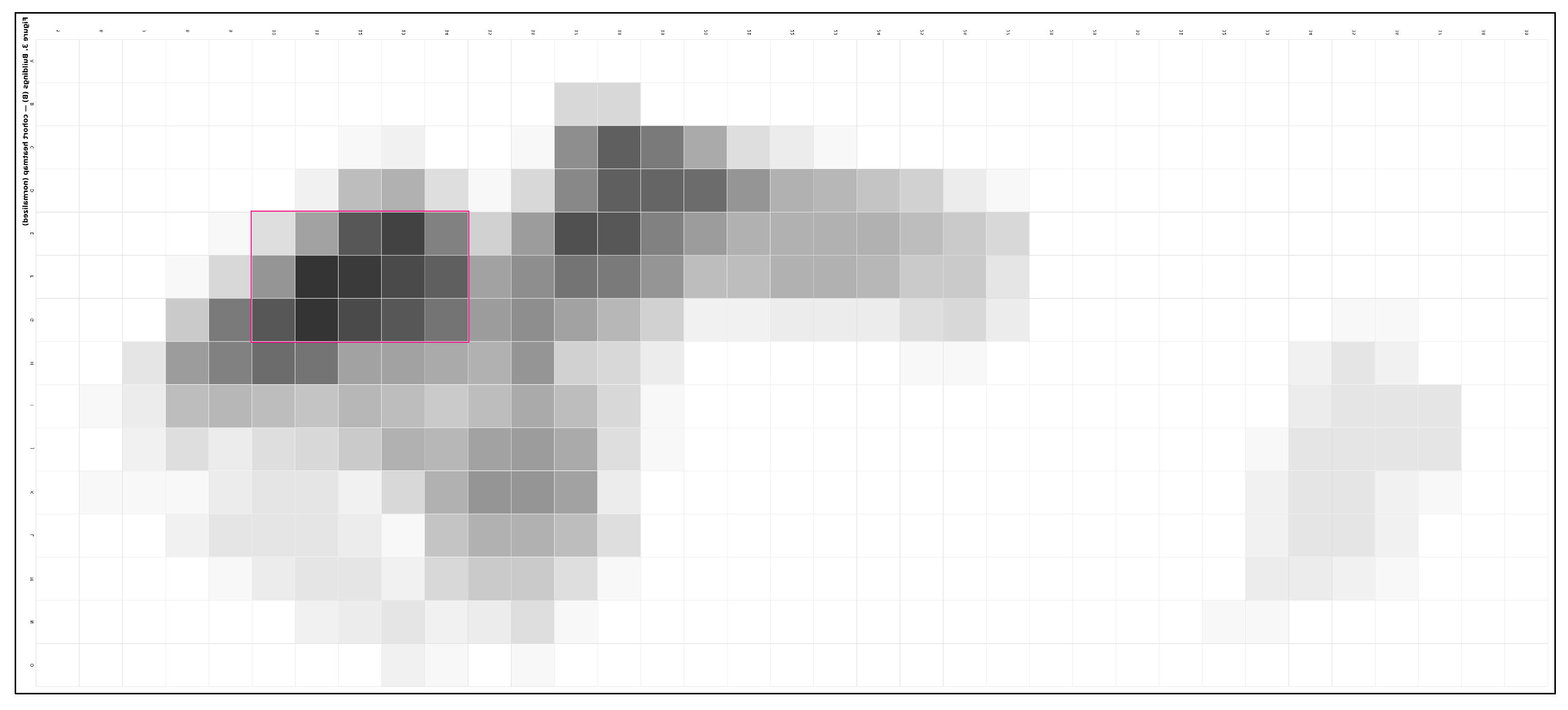
At the cohort scale, building (B) use coalesces into a thick, legible band along the upper-terrace adjacent to the defended wall. The highest-intensity cells cluster in a nucleus centered approximately on E–G / 10–14, where prospect, shelter, and service economy coincide (Figure 6). This nucleus behaves as a plateau rather than a single spike: a two– to three–cell belt tolerates micro-shifts in placement while preserving the same siting logic—edge protection from the wall, elevation for prospect, and proximity to the terrace for efficient access. All coordinates refer to the post hoc analysis grid restricted to the admissible field; distances are in grid units, with meter equivalents provided in the Supplement.
Coverage: Buildings (B) occupy 203/525 (38.667%) cells; Paths (P) occupy 171/525 (32.571%); B ∪ P = 257/525 (48.952%). Exactly 322/525 (61.333%) cells carry zero B-weight, indicating global underutilization and a narrow siting band (Figure 5).
Figure 5.
Combined B (warm) and P (cool) overlays on the admissible field; expert prior outline shown.
Figure 5.
Combined B (warm) and P (cool) overlays on the admissible field; expert prior outline shown.
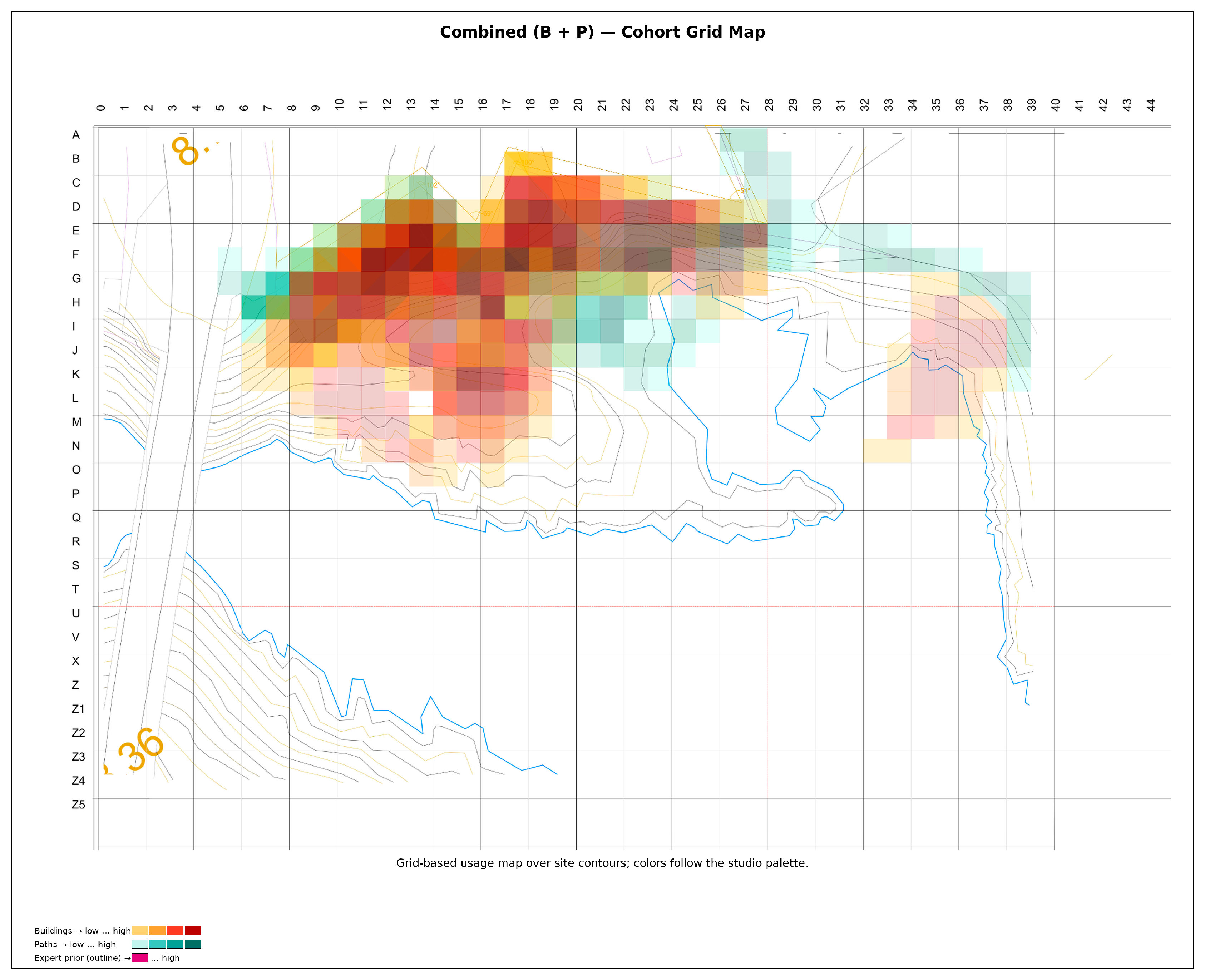
Figure 6.
Building (B) intensity across the cohort on the 15 × 35 grid (A–O × 5–39) over the admissible field. The cohort nucleus along the upper-terrace (E–G / 10–14) is outlined in red. The Colorbar displays the summed B-weights per-cell (N = 22), with no kernel smoothing applied.
Figure 6.
Building (B) intensity across the cohort on the 15 × 35 grid (A–O × 5–39) over the admissible field. The cohort nucleus along the upper-terrace (E–G / 10–14) is outlined in red. The Colorbar displays the summed B-weights per-cell (N = 22), with no kernel smoothing applied.
Nucleus and spine: B—intensity coalesces into a nucleus centered on E–G / 10–14 (upper-terrace, defended wall). P—intensity organizes as a contour-parallel spine along F10–F15, with short stitches that pull movement to/from the nucleus.
Local salience: The top-10 locally salient cells (neighborhood-normalized) have mean z̄ = 1.60 (range 1.37–1.93).
Path structure is organized as a contour-parallel spine along F10–F15, punctuated by short stitches that pull movement to and from the nucleus (Figure 7). Reading the F10–F15 spine as a local axis of continuity and resilience aligns with recent evidence on network connectivity and street-type roles [31,32,33]. The mass–movement coupling is consistent across projects: building mass anchors to the wall–terrace interface; circulation sweeps the bench, minimizing gradient costs while preserving view corridors. Variations arise in where stitches bite into the spine and how the spine bends at terrace hinges, yielding minor but teachable differences in access legibility and processional sequence [4].
Design reading. Projects inside the nucleus show low spread and low breadth (entropy): unambiguous anchoring plus short, high-quality connectors. Projects at the edge of the nucleus show moderate spread as mass “leans” along the terrace; breadth increases slightly to gain lateral prospect while keeping access economical. Projects outside the nucleus exhibit higher spread and breadth, either as deliberate counter-heuristics (e.g., bench habitation, wind shadowing) or as exploratory placements that depend on one or two strong gateways to remain coherent.
Alignment with Expert Prior
We then test whether the cohort sits closer-than-chance to the defended edge–upper-terrace–prospect envelope, and whether building mass is enriched inside that envelope.
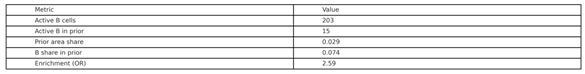
Students’ building centroids were significantly closer to the expert prior than expected by chance. Under the strict prior, the observed mean distance = 3.664 grid units versus a null mean of 10.982 (p < 0.001, ≈ 4.34σ). With a +1-cell buffered prior, the observed mean = 3.002 versus 9.831 (p < 0.001, ≈ 4.10σ). A bootstrap 95% CI for the observed mean (strict prior) is [1.857, 6.094]. Within the prior area (2.857% of grid cells), the cohort concentrates 19.50% of building weight, yielding an odds ratio = 8.237 for inside-versus-outside occupancy. (Table 2).
Interpretation for practice: a lower mean distance means the cohort tends to the defended edge–upper-terrace–prospect band more than chance; OR > 1 says we use that band more often than a random placement would.
Summary: μ_obs(strict)=3.664; μ_null=10.982; Δ≈4.34σ; μ_obs(+1)=3.002; μ_null=9.831; Δ≈4.10σ; OR=8.237. CLES indicates that a random null replicate is less aligned than the observed cohort in >95% of comparisons.

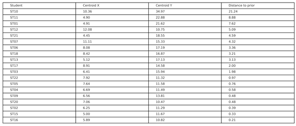
Table 1.
Centroid (cx, cy) and distance to the expert prior for each student.
 |
This result signals robust convergence toward the expert-defined zone—consistent with the studio’s design intent—rather than a pattern explainable by sampling noise (one-sided p < 0.001).
Table 2.
Active prior coverage for Buildings (B) cells and share within the expert prior; estimated enrichment (odds ratio). Note: Odds ratio (OR) reported with 95% CI from bootstrap (B = 10,000).
Table 2.
Active prior coverage for Buildings (B) cells and share within the expert prior; estimated enrichment (odds ratio). Note: Odds ratio (OR) reported with 95% CI from bootstrap (B = 10,000).
 |
4.2. Alignment with the Wall–Terrace–Prospect Logic (Permutation Evidence)
To establish whether the apparent consensus is more than a visual impression, we tested alignment against an explicit expert prior—a polygon encoding defended edge, upper-terrace elevation, and ocean-facing prospect. Using the cohort mean centroid-to-prior distance with a permutation null over admissible cells, the cohort is closer-than-chance (Figure 8; Table 2). Observed mean distance = 3.664 …; with a +1-cell buffered prior, observed mean = 3.002. One-sided p < 0.001 in both cases; see Table 2 for the complementary mass-overlap enrichment (OR = 8.237). We use M = 2,000 permutations in the main text (M = 10,000 in the Supplement), with fixed seeds. Exact one-sided p-values are reported; overlap effect sizes (OR, 95% CI) appear in Table 2. Robustness to buffered and data-driven priors holds (Figure S6; Table 2). A +1-cell buffered prior (registration tolerance) yields consistent conclusions (Figure S6). A data-driven prior (top decile of B-weighted cells) converges on the same qualitative result, showing that the expert prior is consonant with cohort behavior rather than determinative of it (Table 2). Reported p-values are exact (permutation), and standardized effect sizes quantify practical magnitude alongside significance; distances and overlaps converge under multiple seeds (see Supplement).
For practice, “lower mean distance” means the cohort tends to the defended edge–upper-terrace–prospect band more than chance; OR > 1 means we use that band more often than a random placement would.
A complementary mass-overlap proportion—the share of each project’s B mass lying inside the prior—confirms the alignment, with 95% confidence intervals showing overlap levels systematically higher than uniform placement would predict. All inference is at the project level (cohort means of distances or overlaps) to avoid per-cell multiple testing; meter equivalents for distances are documented in the Supplement.
Architectural meaning. “Closer-than-chance” translates into accountable siting. Most proposals are not just near the wall; they are within a terrain-and-exposure-aware envelope that a practitioner might sketch at briefing. The test does not prescribe that envelope; it confirms a shared heuristic that can be taught, debated, defended, or resisted.
4.3. Locally Dominant Connectors: Rescuing Short But Decisive Moves
Global counts obscure key short segments; a local, percentile-based salience perspective reveals ridge-crossings, stitches, and gateways that convey structural intent—simplifying nuance in paths, where short segments bear significant structural weight.
A local 8-neighborhood salience lens reveals globally rare yet locally dominant connectors—ridge-crossings and contour-parallel stitches—whose removal would materially weaken a scheme (Figure 9, Figure 10). Salience is defined as the empirical percentile of the neighborhood sum across the admissible field; cells at or above the 95th percentile are flagged. These short, locally dominant links are consistent with network-based accounts of accessibility and node attraction in urban layouts. Treating them as first-class evidence helps explain why small stitches can carry disproportionate architectural intent [29,30].
Recurrent high-salience cells arise at E13–F14 (characteristic ridge-crossing), E14–F14 (short stitch consolidating the spine beside the building), and F11–F12 (edge gateway). Two quieter but repeatable service alternatives appear at D13 and G8. Complete neighborhood statistics and the contrast with global ranks (cells that matter locally but not globally) appear in Table S3. Sensitivity checks—larger neighborhoods, binary versus weighted P, and ±25% grid resolution—preserve the identity of key connectors within high Jaccard overlap thresholds, as reported in the Supplement.
Design reading - The regularity “defended edge + upper-terrace elevation + ocean prospect” materializes as a siting nucleus anchored to the wall and a contour-parallel spine of circulation along F10–F15. Short stitches and ridge-crossings (e.g., E13–F14) make the variants legible—where the spine bends and how access “bites” into the mass—without collapsing diversity into averages. Salience guides where to act. Strengthening E13–F14 and F11–F12 stabilizes both nucleus-anchored and boundary-leaning schemes. Pruning low-salience detours reduces cognitive noise without curtailing choice. A Gateway Action Map overlays micro-interventions—thickening a crossing, formalizing a hinge, clarifying a bend—precisely where they are most likely to improve legibility (Figure 9, Figure 10). Because salience is local and percentile-based, these findings remain robust to small registration shifts and parameter adjustments.
4.4. Divergent Placements: Two Instructive Vignettes
A small subset of projects demonstrates that coherence without consensus is achievable when connectors are structurally strong.
Vignette A — “Settled in the slope.” The centroid sits downslope, outside the nucleus. The scheme favors bench habitation and microclimatic protection over permanent prospect. Two short crossings near E13–F14, reinforced by a contour stitch, re-bind the project to the spine. Local salience confirms these links as structural rather than decorative; removing either crossing degrades legibility and service efficiency. These divergences read as shifts in legibility and wayfinding structure within the site, rather than mere geometric outliers [27].
Vignette B — “Promontory bias.” The centroid projects seaward beyond the nucleus, privileging long views and a bolder silhouette. Exposure rises, but a single decisive connector near F14–F15 pulls the scheme back into the shared circulation grammar. A second, shorter stitch provides fault-tolerance if the primary connector is compromised by program or phasing.
Vignettes highlight the two most considerable deviations and the gateways that sustain them (Figure 11). Per-student centroid distances and mass-overlaps appear in Table 3; outliers read as distance outliers but connector insiders—formal exceptions that still obey the cohort’s connective rules. Exact values and 95% CIs are reported in Table 1; distances are in grid units with meter equivalents in the Supplement.
4.5. Solution Families (Focus–Spread–Breadth Typology)
Clustering the focus–spread–breadth triplet yields four interpretable siting stances rather than opaque clusters, with internal validity and bootstrap stability. Clusters are obtained by k-means on z-standardized features [focus, spread, breadth] with k-means++ initialization (n_init=100, max_iter=300); k selected by average silhouette and cross-checked with Davies–Bouldin (stability in Figure S4). Validity is assessed with internal metrics to avoid over-interpreting arbitrary partitions [37,38].
Type I — Deep (Concentrated Edge Anchor).
Sectional implication: favors a thick edge with service depth and sheltered courts; short, high-quality gateways deliver legible processional entries.
Type II — Extended (Arm-Aligned).
Sectional implication: reads as a linear promenade along the bench; mass elongation increases prospect but requires disciplined service docking.
Type III — Fragmented (Benched Scatter).
Sectional implication: multiple stepped volumes demand structural gateways to avoid noisy access and to keep the spine intelligible.
Type IV — Prospect-Led (Promontory Bias).
Sectional implication: decisive stance toward viewpoint; exposure and reach are constraints mitigated by dual connectors to the spine.
The family patterns align with compact descriptors previously used to read urban form and solution sets, supporting interpretable typologies rather than opaque labels [7]. Families were obtained by k-means as specified in Section 3.9. We favor readable families over opaque clusters: labels are assigned by architectural stance in the focus–spread–breadth space and validated for internal consistency. Bootstrap Jaccard stability in the Supplement shows Types I–III as stable; Type IV appears when the cohort contains enough promontory-led proposals. The family scatter and diagnostics are shown in Figure S4.
Pedagogical reading. Each family activates actionable questions: Deep—Which gateway is structural? Extended—Where should elongation stop before clarity erodes? Fragmented—Which stitches make fragments read as one figure? Prospect-led—What is the minimum back-connector that keeps service legible?
4.6. Interpretive Summary
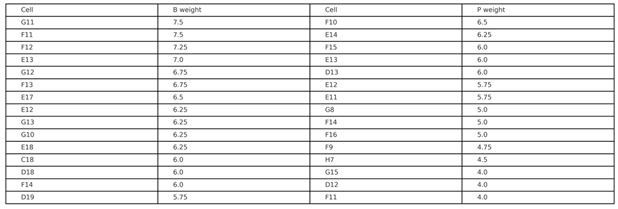
The cohort activates about half of the admissible grid, concentrates building around E–G / 10–14, and relies on a contour-parallel path spine with a handful of high-salience connectors (Figure 5, Figure 6, Figure 7 and Figure 9; Table 1). The top-ranked building cells, ranked by global weight, are G11 and F11 (7.50 each), followed by F12 (7.25), E13 (7.00), and G12/F13 (6.75) (Table 3). Alignment to the concealed expert prior is closer-than-chance and robust to buffered variants and seeds; a complementary mass-overlap view reaches the same conclusion (Figure 8; Figure S6; Table 2). Divergent placements remain architecturally legible when they invest in structurally significant connectors (Figures 9—11; Table 3; Table S3). All permutation results use M = 2,000 in the main text (M = 10,000 in the Supplement), with fixed seeds; exact p-values and standardized effect sizes are reported in captions and tables; meter conversions are provided in the Supplement.
What the evidence adds. Beyond naming a consensus, the analysis makes the consensus accountable (explicit prior), rescues minority intelligence (salience of short connectors), and organizes variety (solution families). Interpretive claims remain bounded by the observational design: we report evidence of alignment and concentration, not causal effects. The studio-facing value lies in transparent prompts for critique and targeted exploration. For educators, this transforms tacit situational knowledge into sharable, testable heuristics; for students, it enhances metacognitive awareness of patterns already in use; for practice, it provides a lightweight baseline for briefing and early option screening without prescribing a single answer.
4.7. Robustness and Sensitivity Overview (Reader-Facing Synthesis)
Findings are robust to grid resolution (±25%), seed choice, and admissible mask variants; permutation p-values and effect sizes remain within the same interpretive band. Buffered and data-driven priors preserve the ‘closer-than-chance’ conclusion. The nucleus/spine pattern and key connectors persist, with high Jaccard overlaps for salience sets. Family labels are stable under bootstrap resampling for Types I–III [37,38]. Three robustness axes were probed to ensure that findings are not artifacts of modeling choices. Prior definition - A buffered prior (+1-cell) and a data-driven prior (top decile of B) maintain the closer-than-chance conclusion for centroid distances and mass-overlaps, indicating that alignment is not contingent on a single envelope geometry (Figure S6; Table 2). Grid resolution - Re-running the pipeline at ±25% cell size preserves the nucleus/spine pattern and the identity of key connectors, with high Jaccard overlaps for the salience sets (Supplement). Clustering stability. The solution-family partition is label-stable under bootstrap resampling for Types I–III; Type IV appears consistently in cohorts with sufficient proposals led by promontory (Supplement). These checks support the substantive reading: the edge–prospect anchoring and its connective grammar are stable features of the cohort’s siting behavior, not artifacts of the discretization or parameterization.
5. Discussion
5.1. What the Cohort Reveals and How It Reframes Critique
For critique, this becomes a five-minute read: locate the nucleus, trace the spine, name the gateway and the stitch, and check if the scheme is closer-than-chance to the defended band—or a valid exception sustained by strong connectors. Collectively, these tests indicate a robust, non-random convergence toward the expert-defined optimal zone (p < 0.001 under both strict and buffered analyses), an enrichment by a factor of approximately 8.24 within the prior area, and a locally concentrated use, as evidenced by a top-10 salience z-mean of 1.60. The cohort converges on a readable grammar of edge–prospect anchoring and a contour-parallel spine for circulation. Building mass concentrates in a siting nucleus centered approximately on E–G / 10–14, while paths form a directional arm around F10–F15 with short stitches to and from the nucleus (Figure 6 and Figure 7). About 61% of the admissible cells receive no building weight (Figure 5), indicating global underutilization and a narrow band of perceived opportunity under the given brief. Read through focus–spread–breadth, nucleus schemes show low spread and breadth (decisive anchoring), boundary schemes trade anchorage for panoramic reach, and out-of-nucleus schemes rely on a few structurally critical connectors to cohere. Making these regularities visible converts tacit know-how into pattern literacy and relocates critique from taste to evidence. Our findings reveal a cohort nucleus along the defended edge, with a directional path spine that aligns with the site-led expert’s prior. Evidence combines exact permutation p-values with standardized effect sizes and 95% BCa intervals, foregrounding magnitude and uncertainty rather than headlines [35,39]. We keep interpretations observational and site-specific. Heatmaps and Top-cell summaries make these selectivities auditable at the cohort scale rather than subjective [4].
Cohort grammar: The cohort converges on edge–prospect anchoring and a contour-parallel spine, a grammar that is interpretable on drawings and auditable in data.
Pedagogical value: The encodings (B/P layers, local salience, focus–spread–breadth) double as a metacognitive scaffold for teaching: a short checklist (‘How to read your siting’) and a Gateway Action Map turn insights into actionable moves. Where is the nucleus? 2) Where does the spine run (contour-parallel)? 3) Which gateway is structurally necessary? 4) Which stitch is essential? 5) What do you lose if you remove that gateway or stitch? (Cross-check with local salience ≥ 95th percentile.) Mini-rubric (0–2 pts each): clarity of nucleus; quality of spine; pertinence of gateway; coherence of stitches; justified alignment or deviation from the defended prior. (Deviations are welcome when backed by strong connectors.)
Limitations and validity: The design is post hoc, observational; we report alignment and concentration, not causation. External validity is pursued through protocol portability and full reproducibility; future work should link siting metrics to process traces (e.g., gaze) and test prospective feedback interventions.
5.2. Teaching Elevation as a Falsifiable Heuristic
Elevation is taught as a hypothesis, not a rule: an independent expert prior plus permutation nulls make acceptance or principled deviation accountable. Here, wall + upper-terrace elevation + ocean prospect behaves as a default heuristic, not a rule. An explicit, site-led expert prior formalizes that intuition and, with a permutation null, turns “closer-than-chance” into a falsifiable statement (Figure 8, Table 2). Using permutation nulls keeps inference distribution-free and controls for the admissible field; a stratified-by-elevation variant preserves broad site structure [35]. Because the prior is independent of student work and buffered variants are reported (Figure S6), teaching elevation becomes an accountable hypothesis students can accept, refine, or overturn using setbacks, connectors, and service costs—keeping computation in service of architectural reading.
5.3. Minority Intelligence and Principled Deviation
A small set of proposals sits downslope or projects toward the promontory. These remain coherent when they invest in locally dominant connectors—ridge-crossings and gateways flagged at ≥95th local percentile (e.g., E13–F14, E14–F14, F11–F12; Figure 9, Table S3). The design lesson is precise: what distinguishes robust deviation is not distance from the nucleus but the strength and placement of connectors. Salience is a local, percentile-based lens, making findings tolerant to minor registration errors and neighborhood choices. This pattern is consistent with network accounts of accessibility and node attraction in street layouts [29,30]. Short, locally dominant connectors often explain why small stitches carry outsized architectural intent.
5.4. From Studio Patterns to Practice: Lightweight Decision Support?
We translate these cohort readings into a 15–30-minute decision lens for early briefing without prescribing outcomes. Cohort-scale evidence can be turned into decision lenses that are fast enough for early briefing without prescribing outcomes. The explicit expert prior (edge–upper-terrace–prospect), the cohort heatmaps, and the focus–spread–breadth descriptors make siting judgments auditable: we can (i) quantify whether a proposal sits closer-than-chance to the site-led hypothesis (centroid-to-prior + permutation null), (ii) verify enrichment of building mass inside the prior (mass-overlap), and (iii) surface structural connectors (gateways, stitches, ridge-crossings) via local salience. The result is not a rulebook but a compact reading scaffold that helps teams discriminate between options early.
Lightweight workflow (15–30 min per option).
- Draw a site-specific prior mask (and a +1-cell buffered variant).
- Encode the option on the neutral grid (B/P layers) and compute focus–spread–breadth.
- Read alignment: centroid-to-prior and mass-overlap (report the enrichment ratio and the one-sided permutation p).
- Map local salience to confirm that at least one connector (gateway/stitch) is structurally justifying the placement.
- Compare options by pattern fit (nucleus & spine legibility) rather than averages; keep divergent proposals when supported by strong connectors.
What it answers in practice.
- Where should the nucleus sit? — favoring the defended edge/upper-terrace band when justified by alignment and enrichment.
- How does movement read? — a contour-parallel spine with explicit gateways; absence of connectors is a red flag.
- Is variety coherent? — spread/breadth outside the cohort envelope signals fragmentation unless stitches are strong.
- Are we over- or under-using the field? — heatmaps reveal neglect vs. overcrowding, guiding brief calibration.
- Traffic-light read (calibrate to each site).
- Green: observed centroid-to-prior distance clearly below the permutation null; enrichment » 1 inside the prior; at least one high-salience connector anchors the scheme.
- Amber: mixed signals (alignment without connectors, or connectors without enrichment); revisit gateway location and breadth.
- Red: farther-than-chance placement with no structural connector; treat as a deliberate exception if defended by program or performance criteria.
This is post hoc, observational pattern evidence—use it to inform critiques and brief adjustments, not to replace performance analysis (microclimate, access, heritage) or regulatory compliance [4]. Always test alternative priors (strict/buffered/variant) and keep minority intelligence when its connectors are structurally sound; evidence should expand the teachable set, not narrow it [6].
5.5. Pedagogical Routines and Assessment
Two simple routines are ready for adoption. A pattern-read critique asks: Where is the anchor? Which gateway is structural? Which stitch can be pruned without loss? A vignette iteration selects one intervention from the Gateway Action Map, applies it, and re-reads focus–spread–breadth (“did focus drift? did spread/entropy shrink?”). For assessment, focus indexes siting intent, spread reads spatial economy, and breadth separates exploration from drift. These measures do not grade style; they make criteria explicit and comparable across cohorts, supporting fairer feedback. These routines complement recent studio technologies—VR/BIM frameworks and learning-analytics dashboards—while keeping design reasoning central [16,18].
5.6. Validity and Limits (with Safeguards)
The posture is post hoc and observational; claims are descriptive/associative, not causal. Safeguards include project-level inference (respecting spatial dependence); a falsifiable expert prior tested against a permutation null (M = 2,000 in the main text; M = 10,000 in the Supplement) with fixed seeds; a mass-overlap complement with 95% CIs; buffered and data-driven prior variants; and a public configuration for byte-for-byte reproduction. Internal cluster validity is reported to avoid over-interpreting arbitrary partitions (average silhouette; Davies–Bouldin) [37,38]. Confidence intervals use BCa bootstrap with declared resampling size, and permutation tests use fixed seeds (M as stated above) [35,39]. Limits remain: a single site archetype (coastal terrace with defended wall), finite grid resolution (15 × 35) tempered by ±25% checks (see Figure S1-S11 for grid-size sensitivity), an admissible-mask rule set (Supplement), and the absence of process traces (think-aloud, gaze). This bound scope, not its usefulness: the protocol yields a public baseline that others can replicate, extend, or dispute.
For design education, the protocol also opens a path to cohort-level reflection. By visualizing shared tendencies and exceptions, students can critically recognize their own heuristic anchors and expand the range of siting options discussed in studio.
5.7. Relation to Prior Work (What This Adds)
This study threads semantic encodings, pattern documentation, and visual analytics at the site scale. It adds three elements rarely combined: (i) a quantitative referential for cohort-scale siting heuristics with an explicit, portable expert prior; (ii) a metacognitive scaffold that equips studios with names, measures, and tests; and (iii) a readable focus–spread–breadth typology that organizes variety without collapsing it into averages. It builds upon earlier work on computational ontologies, formulation–generation–evaluation pipelines, public-space patterns, and data-driven typologies by delivering a lightweight, auditable protocol tailored to studio conditions. It consolidates strands on computational ontologies, formulate-generate-evaluate pipelines, public-space patterns, and data-driven typologies into a single, readable protocol for siting at studio scale [6,13,40,41].
This positioning directly addresses the Special Issue on Emerging Trends in Architecture by combining studio-scale visual analytics with reproducible, practice-transferable siting evidence.
5.8. Research Directions Opened by the Protocol
Three immediate paths follow. Causal: randomize or stagger exposure to cohort analytics under a standardized brief; preregister metrics (centroid-to-prior distance, mass-overlap, dispersion) and the analysis plan. Cognitive: layer think-aloud and exit micro-surveys on the same grid to track which cues (edge protection, prospect, access economy) students invoke and how they justify exceptions. Comparative: replicate across site archetypes (coastal terrace, river valley, urban grid) and programs to assemble a comparative atlas of siting heuristics. Pre-registration of metrics and analysis plans will strengthen claims and reduce the researcher's degrees of freedom [35].
5.9. Methodological Extensions while Preserving Interpretability
Extensions should remain legible to designers: stratified permutations by elevation; bootstrap Jaccard for cluster stability; simple network descriptors of paths (gateways, crossings) as a complement to salience; optional local Moran’s I in the Supplement to check spatial structure; and hierarchical/mixture models that capture heterogeneity without forcing consensus. For alignment with the spatial analysis literature, we include in the SI a local association sanity check using Local Moran’s I (LISA) following the classical framework in [24]. Grid sensitivity, prior, and seeds should remain reported, not hidden.
5.10. Implementation Guidance for Practice and Ethics
Use the protocol when early siting choices are contentious, high-stakes, or involve multiple stakeholders. Keep the expert prior independent of advocacy teams to avoid anchoring and disclose its logic (edge, elevation, prospect) in plain language. Treat divergent schemes as informative counter-hypotheses, not errors. Archive the config.json, figures, and summary tables with meeting minutes to ensure accountability. Avoid overconfidence: the lens clarifies choices, not prescribes a single answer.
5.11. Closing Note
The contribution is a clear lens, not a new algorithm. By turning cohort work into shareable evidence, the approach strengthens critique, increases awareness of the patterns architects already use, and makes early siting judgments accountable—without mistaking evidence for prescription. That standard is one a studio can sustain and a practice can adopt when it needs to explain why this building belongs here.
6. Conclusions
This protocol converts studio outcomes into shareable, testable evidence at the site scale—portable across sites and cohorts and ready for cross-studio comparison. Across 22 projects, we find a consistent heuristic—edge–prospect anchoring, linked by a contour-parallel spine-accounted for through permutation-based alignment to an explicit, site-led prior. The same encodings (grid B/P layers, local salience, and the focus–spread–breadth triplet) function as a metacognitive scaffold for teaching and as lightweight decision support in briefing, without prescribing a single solution. Principled deviations remain legible when connectors are structurally strong, expanding rather than narrowing the teachable set. Because the protocol is site-agnostic and released with a replication pack, it now supports cross-studio comparison and enables prospective, controlled studies on when and why feedback shifts siting.
Because the prior is an explicit mask, the protocol is applied in other locations with comparable logic (cliffs, escarpments, arboreal curtains), where one redraws the envelope and tests whether the cohort approaches it more than chance. This framework facilitates cross-studio comparisons presently and allows for future controlled studies on the timing and rationale behind feedback-induced shifts in siting. In this sense, cohort-scale siting evidence can feed urban typology discovery, extending indicator-based comparability from studio proposals to district/block families (see [7]).
Thus, the method expands studio discourse: it keeps well-argued exceptions while making common patterns transparent and comparable across cohorts.
Supplementary Materials
The following supporting information can be downloaded at the website of this paper posted on Preprints.org. Figures S1–S11 (site grid & prior; cohort B/P maps; combined activity; centroids; local salience; permutation null; student vignettes ST15, ST02, ST10, ST11) and Tables S1–S7 (coverage; top-15 cells; prior enrichment; centroid distances; salience top-10; typical & divergent cases).
Funding
This research was supported by the Foundation for Science and Technology (FCT), Lisbon, Portugal, under the co-financed contract CEECINST/00112/2018/CP1530/CT0014.
Author Contributions (CRediT)
Conceptualization, N.M.; Methodology, N.M.; Software, V.M.; Validation, N.M.; Formal analysis, V.M. and N.M.; Investigation, N.M. and V.M.; Data curation, N.M.; Visualization, V.M.; Writing—original draft, N.M.; Writing—review & editing, N.M.; Supervision, N.M.; Project administration, N.M.; Funding acquisition, N.M. All authors read and agreed to the published version.
IRB Statement
Not applicable. The study analyzes anonymized coursework artifacts and does not involve human subjects research.
Informed Consent Statement
Not applicable.
Data Availability Statement
All data and code are available at https://doi.org/10.5281/zenodo.17433474 (Replication Pack: config, machine-readable CSVs, sample B/P encodings, and SHA-256 manifest). Visual vignettes and figure panels are provided as Supplementary Materials with the journal.
Acknowledgments
We thank participating students and colleagues for relevant discussions. Figure 2a reproduced with permission from the Cascais Municipal Archive/ date and author unknown.
Use of Generative AI
A language model assisted with editing and organization only; data coding, statistics, figures, and interpretations were produced and verified by the authors.
Conflicts of Interest
The authors declare no conflict of interest.
ORCID. Nuno Montenegro: 0000-0001-8520-7905; Vasco Montenegro: [to be provided].
Abbreviations
B = Buildings (mass); P = Paths; OR = Odds Ratio; CLES = Common Language Effect Size; BCa = Bias-Corrected and Accelerated (bootstrap).
References
- C. Norberg-Schulz, Genius Loci: Towards a Phenomenology of Architecture. New York: Rizzoli, 1980.
- D. A. Schön, The Reflective Practitioner: How Professionals Think in Action. Abingdon: Routledge, 2017. [CrossRef]
- B. Lawson, How Designers Think: The Design Process Demystified, 4th ed. Oxford: Architectural Press, 2005. [CrossRef]
- Z. Zhang, Y. Xiao, X. Luo, and M. Zhou, “Urban human activity density spatiotemporal variations and the relationship with geographical factors: An exploratory Baidu heatmaps-based analysis of Wuhan, China,” Growth Change, vol. 51, no. 1, pp. 505–529, Mar. 2020. [CrossRef]
- B. Hillier and J. Hanson, The Social Logic of Space. Cambridge: Cambridge University Press, 1984. [CrossRef]
- J. Duarte, J. Beirao, N. Montenegro, and J. Gil, “City induction: A model for formulating, generating, and evaluating Urban designs,” Communications in Computer and Information Science (CCIS), vol. 242, pp. 73–98, 2012. [CrossRef]
- J. Gil, J. N. Beirão, N. Montenegro, and J. P. Duarte, “On the discovery of urban typologies: Data mining the many dimensions of urban form,” Urban Morphology, vol. 16, no. 1, pp. 27–40, 2012.
- J. Appleton, The Experience of Landscape, 2nd ed. Chichester: Wiley, 1996.
- I. L. McHarg, Design with Nature, 25th Anniversary ed. New York: Wiley, 1995.
- F. Miranda et al., “The State of the Art in Visual Analytics for 3D Urban Data,” Computer Graphics Forum, vol. 43, no. 3, 2024. [CrossRef]
- Z. Deng, D. Weng, S. Liu, Y. Tian, M. Xu, and Y. Wu, “A survey of urban visual analytics: advances and future directions,” Comput Vis Media (Beijing), no. 9(1), pp. 3–39, 2023. [CrossRef]
- N. Montenegro, J. C. Gomes, P. Urbano, and J. P. Duarte, “A Land Use Planning Ontology: LBCS,” Future Internet, vol. 4, no. 1, Jan. 2012. [CrossRef]
- N. Montenegro, J. Beirão, and J. Duarte, “Describing and locating public open spaces in urban planning,” International Journal of Design Sciences and Technology, vol. 19, no. 2, 2012.
- N. Montenegro, “Integrative Analysis of Text-To-Image Ai Systems in Architectural Design Education: Pedagogical Innovations and Creative Design Implications,” Journal of Architecture and Urbanism, vol. 48, no. 2, pp. 109–124, 2024. [CrossRef]
- E. Vermisso, “Fragmented Layers of Design Thinking: Limitations and Opportunities of Neural Language Model-assisted processes for Design Creativity,” Design Computation Input/Output 2022, Oct. 2022. [CrossRef]
- A. Hajirasouli, S. Banihashemi, P. Sanders, and F. Rahimian, “BIM-enabled virtual reality (VR)-based pedagogical framework in architectural design studios,” Smart and Sustainable Built Environment, vol. ahead-of-print, no. ahead-of-print, 2023. [CrossRef]
- R. Oxman, “Thinking difference: Theories and models of parametric design thinking,” Des Stud, vol. 52, pp. 4–39, Sep. 2017. [CrossRef]
- T. Nazaretsky, C. Bar, M. Walter, and G. Alexandron, “Empowering Teachers with AI: Co-Designing a Learning Analytics Tool for Personalized Instruction in the Science Classroom,” LAK22: 12th International Learning Analytics and Knowledge Conference, pp. 1–12, Mar. 2022. [CrossRef]
- C.-C. Wang, C.-L. Wu, L. Dong, L. He, and Z. Xie, “Optimization of Urban Shelter Locations Using Bi-Level Multi-Objective Location-Allocation Model,” International Journal of Environmental Research and Public Health 2022, Vol. 19, Page 4401, vol. 19, no. 7, p. 4401, Apr. 2022. [CrossRef]
- Y. Chen, H. Men, and X. Ke, “Optimizing urban green space patterns to improve spatial equity using location-allocation model: A case study in Wuhan,” Urban For Urban Green, vol. 84, p. 127922, 2023. [CrossRef]
- T. Borba, B., Clemente., A., Nepomuceno, T., Cavalcante, “Optimizing Police Facility Locations Based on Cluster Analysis and the Maximal Covering Location Problem,” Applied System Innovation, vol. 5, no. 4, p. 74, Jul. 2022. [CrossRef]
- R. Alfredo et al., “Designing a Human-Centred Learning Analytics Dashboard In-Use,” Journal of Learning Analytics, vol. 11, no. 3, pp. 62–81, 2024. [CrossRef]
- C. Villa-Torrano et al., “Using learning design and learning analytics to promote, detect and support socially-shared regulation of learning: a systematic review,” Comput Educ, vol. 232, p. 105261, 2025. [CrossRef]
- L. Anselin, “Local Indicators of Spatial Association—LISA,” Geogr Anal, vol. 27, no. 2, pp. 93–115, 1995. [CrossRef]
- S. Porta, P. Crucitti, and V. Latora, “The network analysis of urban streets: a primal approach,” Environ Plann B Plann Des, vol. 33, no. 5, pp. 705–725, 2006. [CrossRef]
- A. Turner, “From axial to road-centre lines: a new representation for space syntax and a new model of route choice for transport network analysis,” Environ Plann B Plann Des, vol. 34, no. 3, pp. 539–555, 2007. [CrossRef]
- K. Lynch, The Image of the City. Cambridge, MA: The MIT Press, 1960.
- D. W. Longley, P.A., Goodchild, M.F., Maguire, D.J. and Rhind, Geographic Information Science and Systems, 4th Edition. Wiley, 2015.
- A. Sevtsuk and R. Kalvo, “Patronage of urban commercial clusters: A network-based extension of the Huff model for balancing location and size,” Environ Plan B Urban Anal City Sci, vol. 45, no. 3, pp. 508–528, May 2018. [CrossRef]
- A. Jiang and C. Claramunt, “Topological analysis of urban street networks,” Environ Plann B Plann Des, vol. 31, no. 1, pp. 151–162, 2004. [CrossRef]
- G. Boeing and J. Ha, “Resilient by design: Simulating street network disruptions across every urban area in the world,” Transp Res Part A Policy Pract, 2024. [CrossRef]
- S. Tsigdinos, G. Salamouras, I. Chatziioannou, E. Bakogiannis, and A. Nikitas, “A worldwide review of formal national street classification plans as a tool for more sustainable cities,” Cities, vol. 154, p. 105371, 2024. [CrossRef]
- C. Barrington-Leigh, “A high-resolution global time series of street-network sprawl,” Environ Plan B Urban Anal City Sci, 2025. [CrossRef]
- A. Shaamala, N. Tilly, and T. Yigitcanlar, “Leveraging urban AI for high-resolution urban heat mapping,” Environ Plan B Urban Anal City Sci, 2025. [CrossRef]
- P. Good, Permutation Tests: A Practical Guide to Resampling Methods for Testing Hypotheses. in Springer Series in Statistics. New York: Springer, 2000. [CrossRef]
- P. Crucitti, V. Latora, and S. Porta, “Centrality measures in spatial networks of urban streets,” Phys Rev E, vol. 73, no. 3, p. 36125, 2006. [CrossRef]
- D. L. Davies and D. W. Bouldin, “A cluster separation measure,” IEEE Trans Pattern Anal Mach Intell, vol. PAMI-1, no. 2, pp. 224–227, 1979. [CrossRef]
- P. J. Rousseeuw, “Silhouettes: A graphical aid to the interpretation and validation of cluster analysis,” J Comput Appl Math, vol. 20, pp. 53–65, 1987. [CrossRef]
- B. Efron, “Better bootstrap confidence intervals,” J Am Stat Assoc, vol. 82, no. 397, pp. 171–185, 1987. [CrossRef]
- N. Montenegro, J. N. Montenegro, J. Gomes, P. Urbano, and J. Duarte, “An OWL2 land use ontology: LBCS,” in Lecture Notes in Computer Science (including subseries Lecture Notes in Artificial Intelligence and Lecture Notes in Bioinformatics), 2011. [CrossRef]
- N. Montenegro and J. P. Duarte, “Computational Ontology of Urban Design: Towards a City Information Model,” eCAADe Proceedings, pp. 253–260, 2009. [CrossRef]
Figure 1.
a-b. Representative 1:100 study models from the studio cohort. Two distinct strategies along the defended wall and stepped terrain: a) hinged landing with ridge-crossing and contour-parallel promenade, b) compact edge anchor with a stitched terrace segment. The sequence illustrates how students coupled architectural massing with slope lines before the analytical encoding used later in the paper.
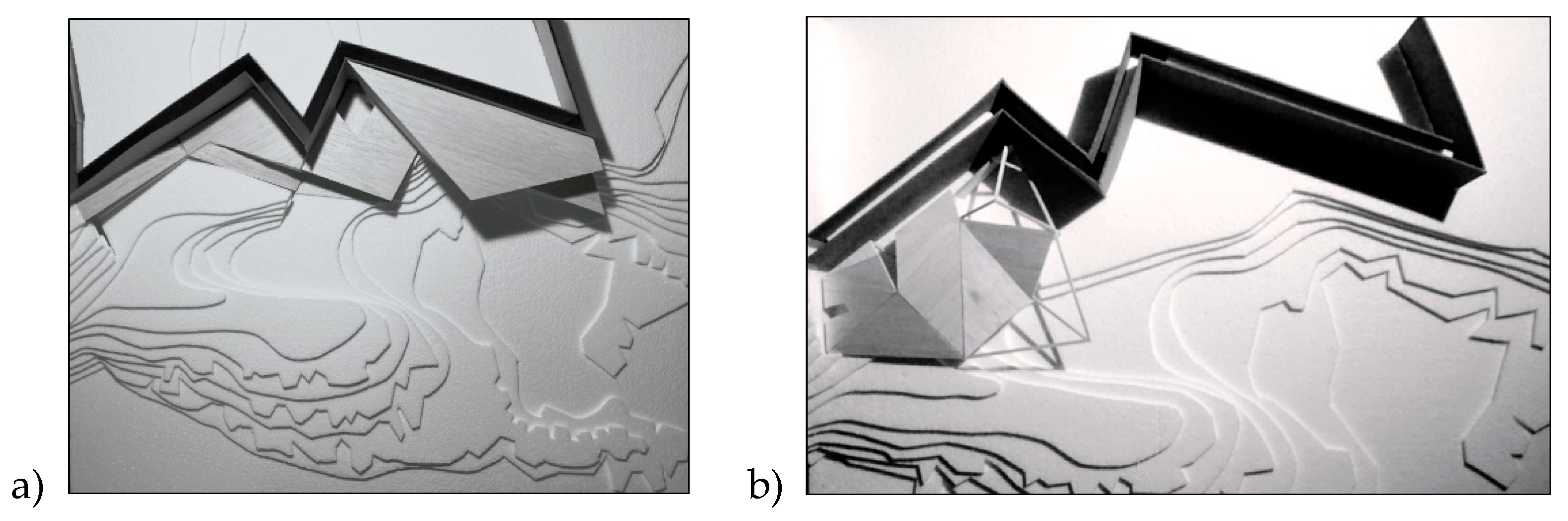
Figure 2.
a-b. Site context. (a) Oblique view of the study area. A—Fortress (17th century); B—Bridge (19th century); C—Opposite shore (20th-century house by architect R. Lino); D—Atlantic Ocean. The red dotted line marks the project intervention area. (b) Analytical site plan with a 15 × 35 grid (A–O × 5–39) over the permitted field (hatched outside), expert prior (solid red), and +1-cell buffer zone (dashed red). A coastal headland marked by a blue line shows the shoreline, with a historic defensive wall depicted in dark grey. Distances are in grid units; meter equivalents and layer origins are detailed in the Supplement.
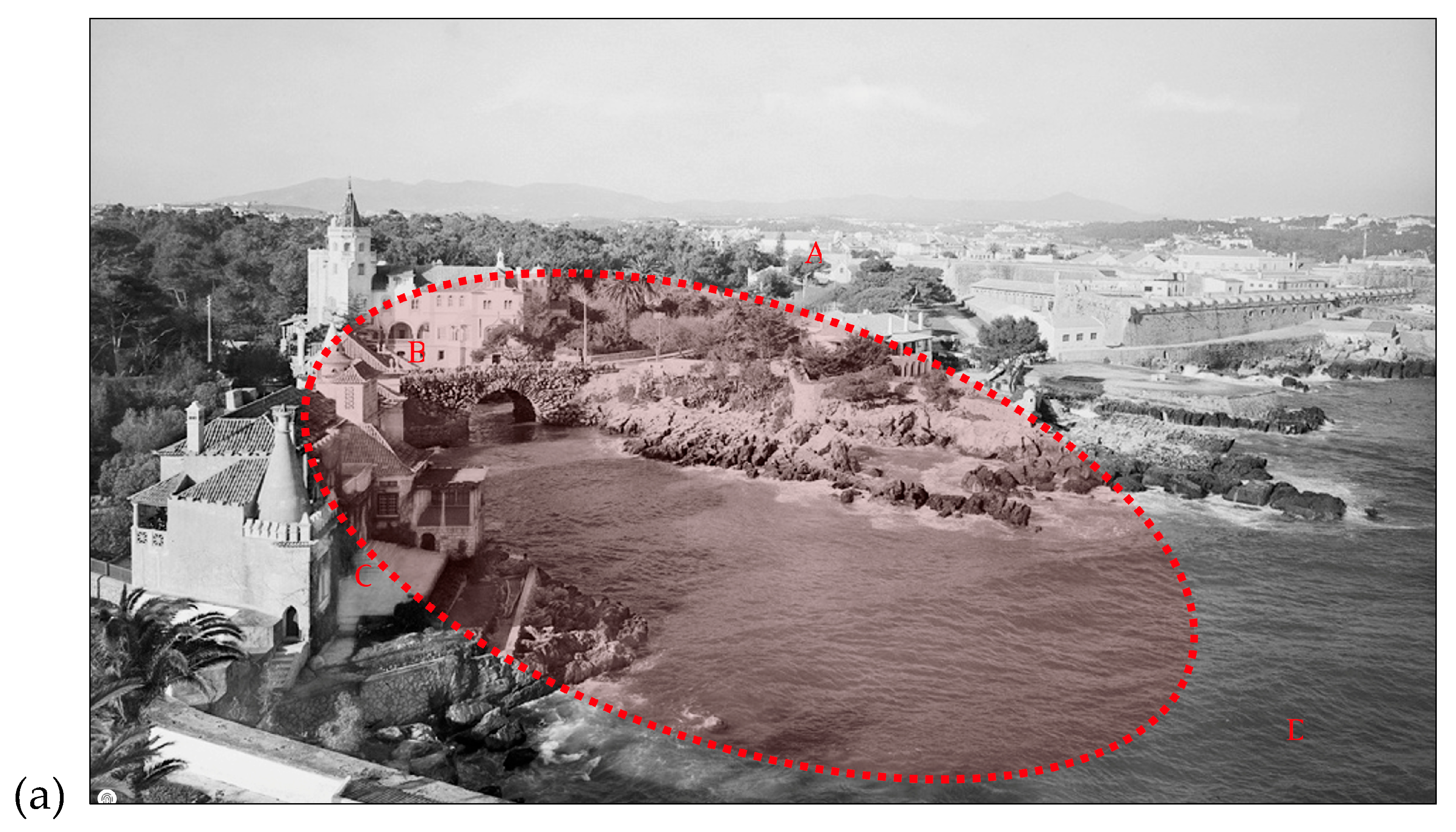
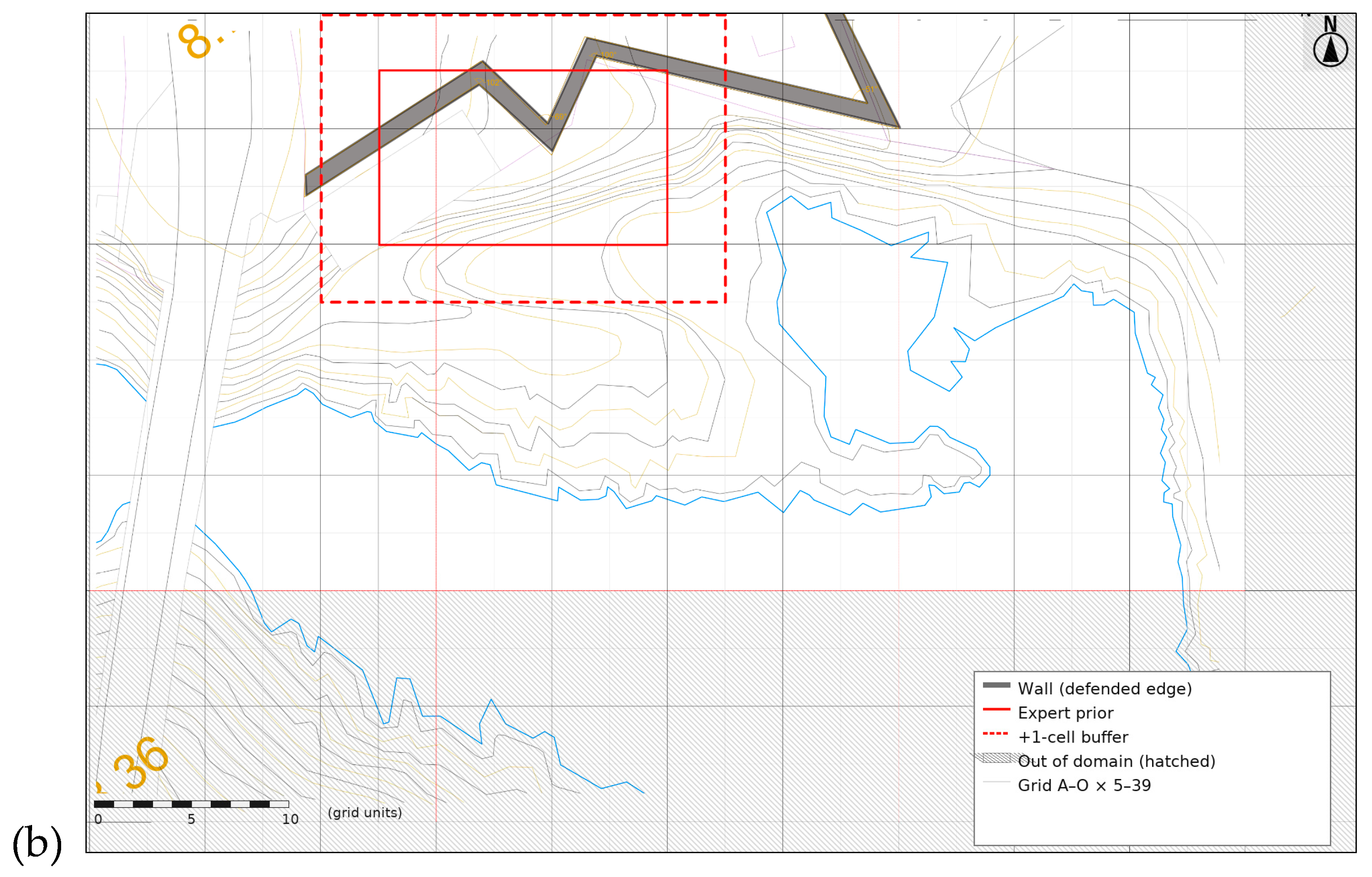
Figure 3.
Analysis workflow. Drawings → grid → B/P encodings → cohort heatmaps → prior-alignment tests → local salience → solution families. Parameters are fixed and reproducible (Replication Pack).
Figure 3.
Analysis workflow. Drawings → grid → B/P encodings → cohort heatmaps → prior-alignment tests → local salience → solution families. Parameters are fixed and reproducible (Replication Pack).
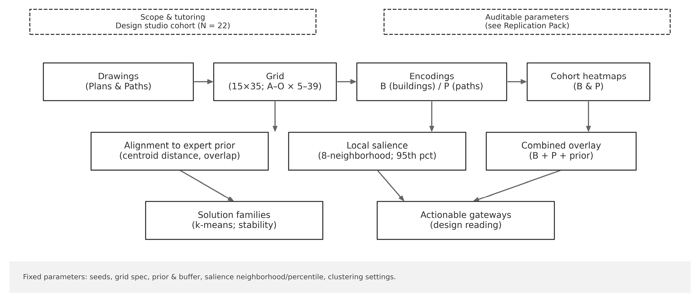
Figure 4.
Pedagogical research framework. Study framework linking studio context, data collection, and pattern extraction (DP = design patterns; LP/MP/VP = location, morphology, views).
Figure 4.
Pedagogical research framework. Study framework linking studio context, data collection, and pattern extraction (DP = design patterns; LP/MP/VP = location, morphology, views).
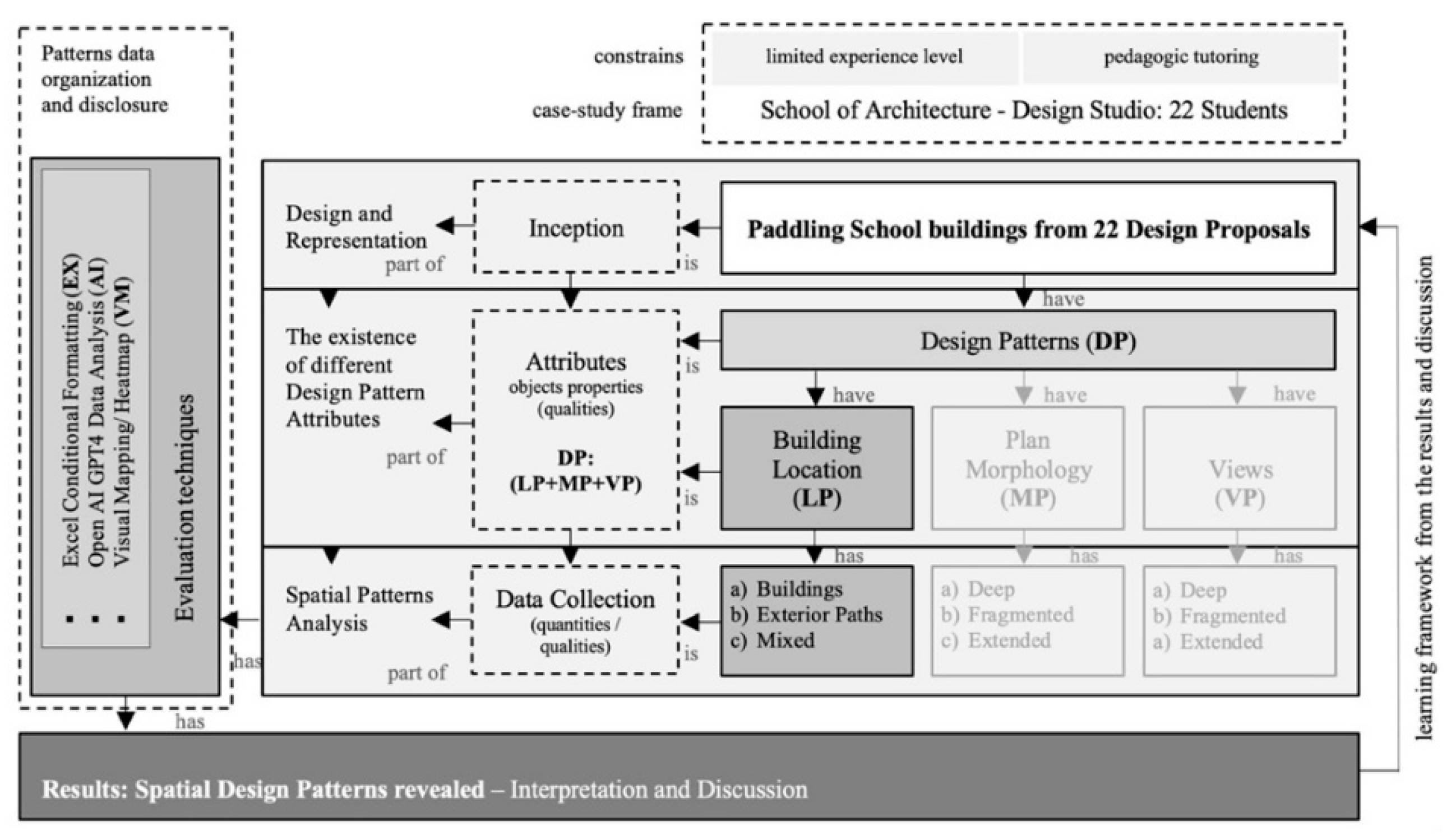
Figure 7.
Path (P) intensity across the cohort. Contour—parallel arm near F10–F15, with short stitches to and from the building nucleus (around F10–F15). Colorbar: summed P-weights (N = 22); no smoothing.
Figure 7.
Path (P) intensity across the cohort. Contour—parallel arm near F10–F15, with short stitches to and from the building nucleus (around F10–F15). Colorbar: summed P-weights (N = 22); no smoothing.
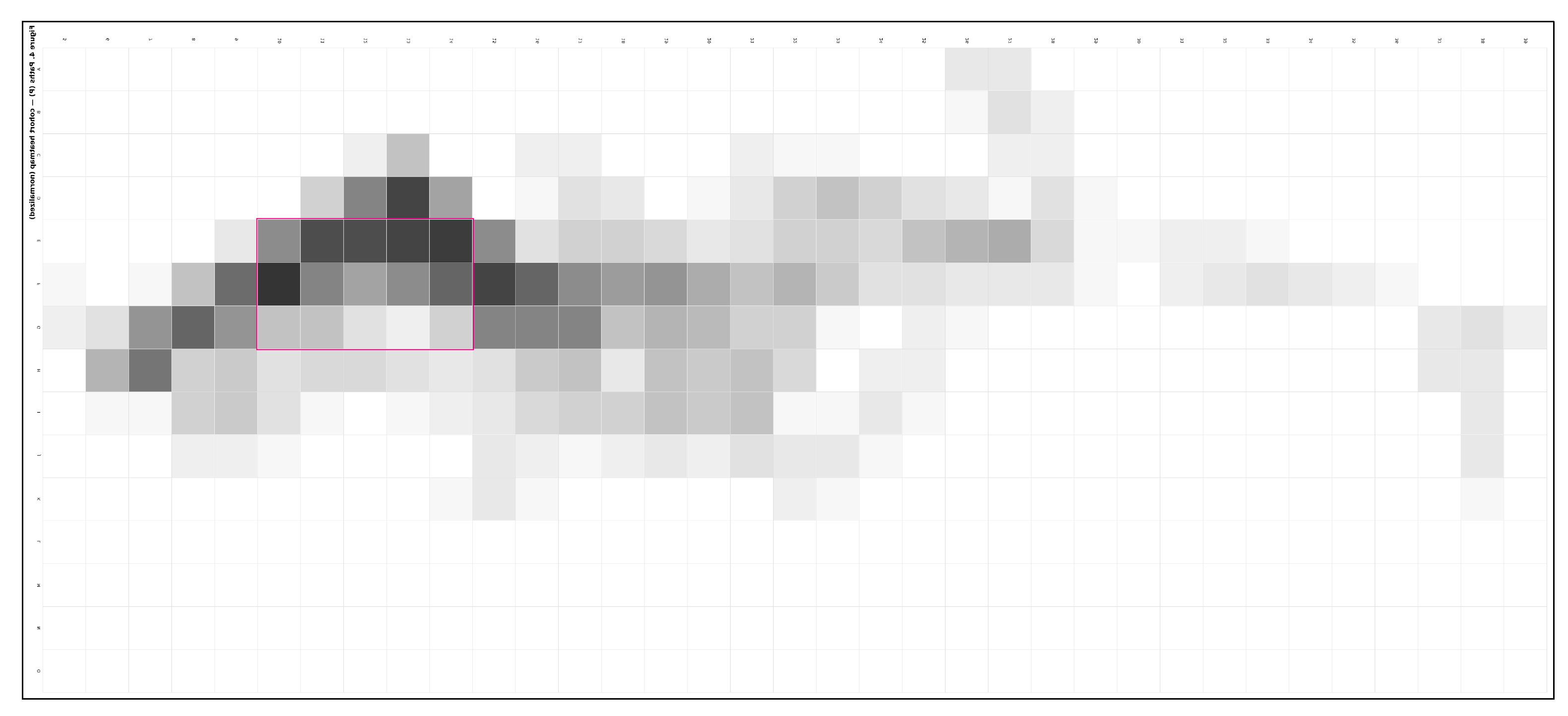
Figure 8.
Permutation null (M = 2,000) for the cohort mean centroid-to-prior distance. The vertical line marks the observed mean (3.664 for the strict prior; 3.002 for the +1-cell buffered prior). One-sided p < 0.001 in both cases; bootstrap 95% CI [1.857, 6.094] for the strict prior.
Figure 8.
Permutation null (M = 2,000) for the cohort mean centroid-to-prior distance. The vertical line marks the observed mean (3.664 for the strict prior; 3.002 for the +1-cell buffered prior). One-sided p < 0.001 in both cases; bootstrap 95% CI [1.857, 6.094] for the strict prior.
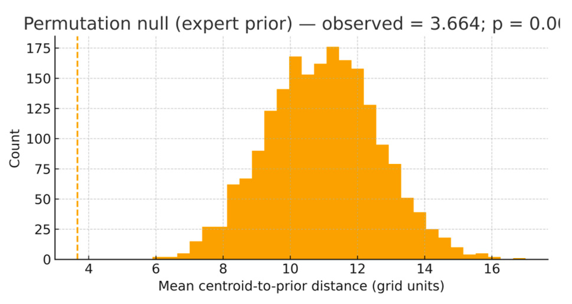
Figure 9.
Paths with local-salience overlay. Top-10 locally dominant connectors highlighted (e.g., E27 highest, z = 1.93).
Figure 9.
Paths with local-salience overlay. Top-10 locally dominant connectors highlighted (e.g., E27 highest, z = 1.93).
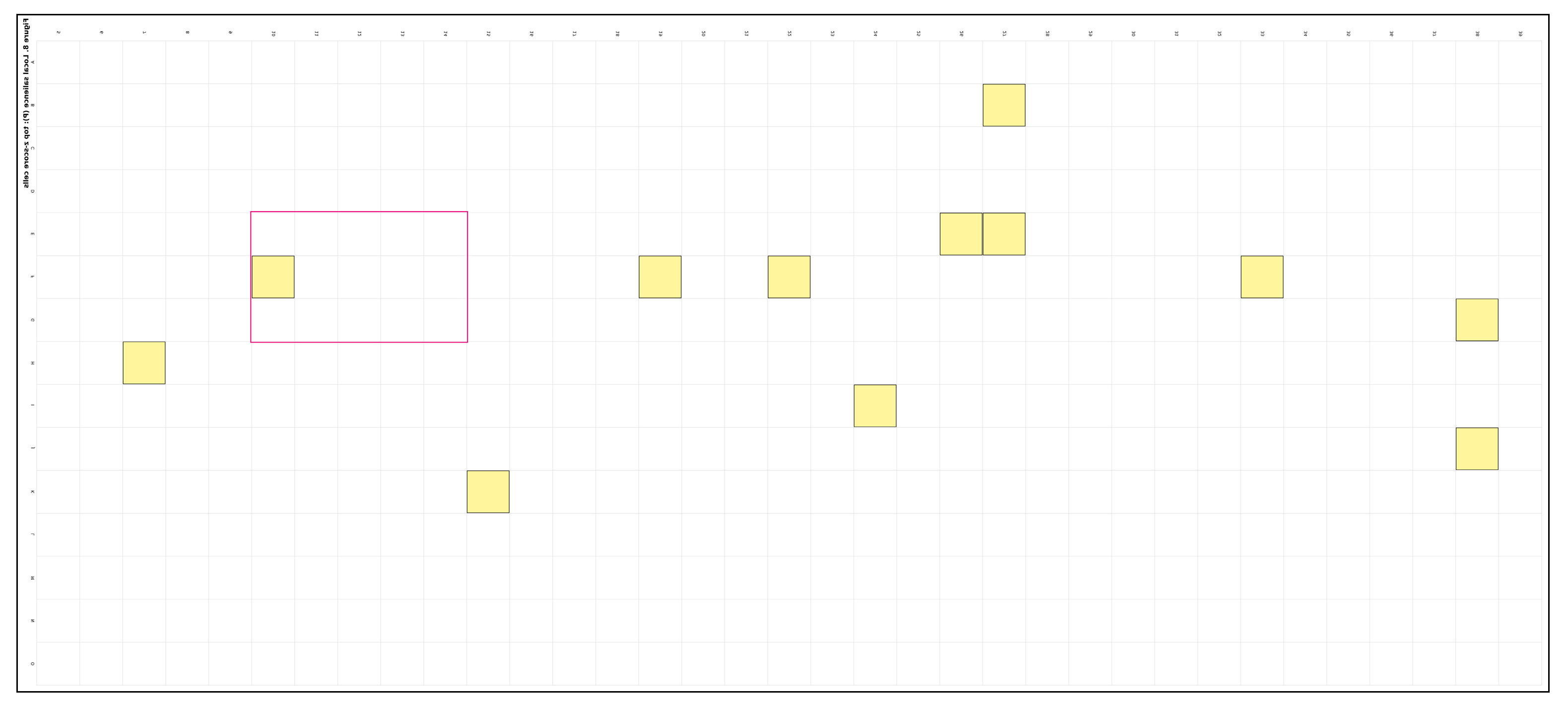
Figure 10.
Paths (P) intensity with local salience overlay on the 15 × 35 grid (A–O × 5–39) over the admissible field. Locally dominant connectors (≥95th percentile). Salient cells within the admissible field; labels at E13–F14, E14–F14, F11–F12, D13, G8.
Figure 10.
Paths (P) intensity with local salience overlay on the 15 × 35 grid (A–O × 5–39) over the admissible field. Locally dominant connectors (≥95th percentile). Salient cells within the admissible field; labels at E13–F14, E14–F14, F11–F12, D13, G8.
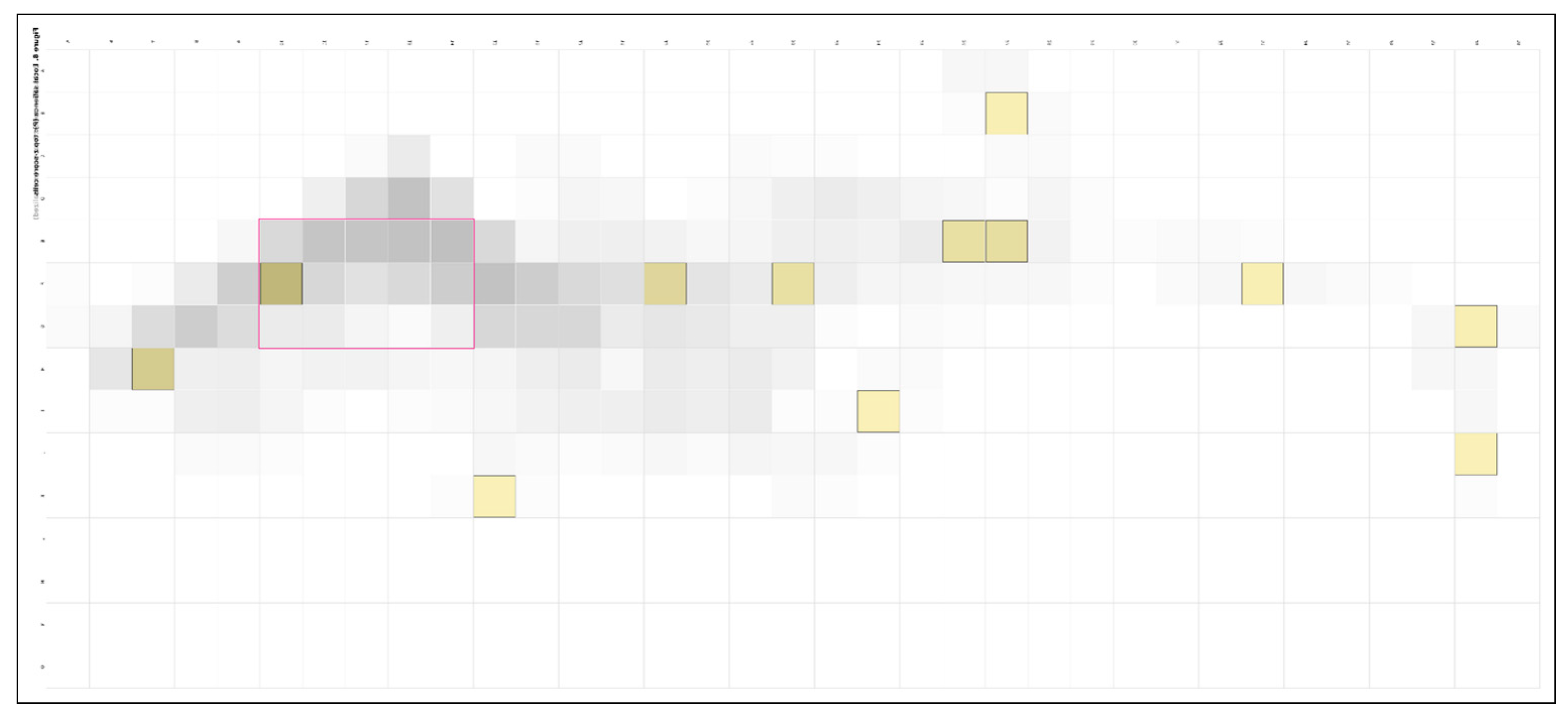
Figure 11.
a-b. Cohort vignettes illustrating typical (edge-anchored, arm-aligned) (left – student S15) and divergent (lower-terrace, ridge-crossings) (right – student S10) solutions.
Figure 11.
a-b. Cohort vignettes illustrating typical (edge-anchored, arm-aligned) (left – student S15) and divergent (lower-terrace, ridge-crossings) (right – student S10) solutions.
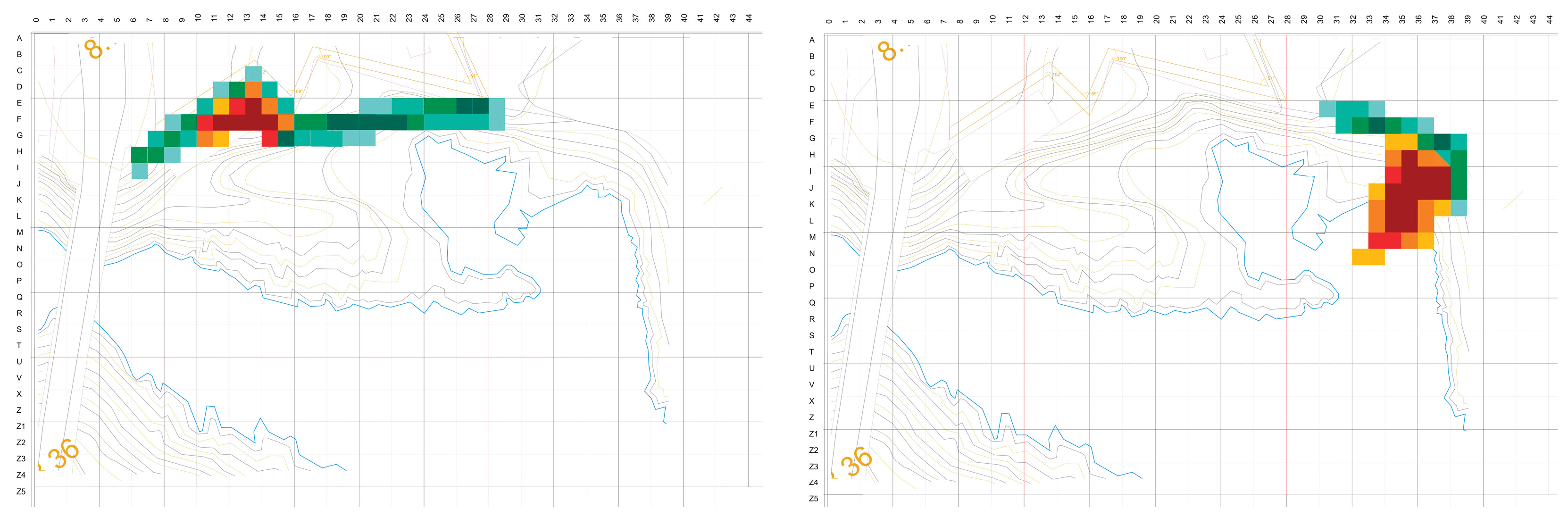
Table 3.
Top-15 admissible cells by weighted usage for B and P layers (N = 22).
 |
Disclaimer/Publisher’s Note: The statements, opinions and data contained in all publications are solely those of the individual author(s) and contributor(s) and not of MDPI and/or the editor(s). MDPI and/or the editor(s) disclaim responsibility for any injury to people or property resulting from any ideas, methods, instructions or products referred to in the content. |
© 2025 by the authors. Licensee MDPI, Basel, Switzerland. This article is an open access article distributed under the terms and conditions of the Creative Commons Attribution (CC BY) license (http://creativecommons.org/licenses/by/4.0/).
Copyright: This open access article is published under a Creative Commons CC BY 4.0 license, which permit the free download, distribution, and reuse, provided that the author and preprint are cited in any reuse.


