Topological Model of Spatial Connectivity: Geometric Anisotropy from G_ik and Cosmological Consequences of Variable c_eff

1. Introduction

The unification of quantum mechanics (QM) and general relativity (GR) remains one of the central unresolved problems of fundamental physics. Beginning with Einstein’s works, numerous attempts have been made to construct a single geometric picture of interactions. However, the known approaches—from classical Kaluza–Klein models to modern string theory [1] and loop quantum gravity (LQG) [2,3]—face a number of difficulties. String theories require additional dimensions and an enormous multiplicity of modes, whereas LQG relies on a discretization of geometry but has not yet produced a self-consistent phenomenology. A common limitation of both directions is the scarcity of testable predictions that go beyond already established observations.

At the same time, within classical GR singularities inevitably arise—black holes, the cosmological singularity—which signal an incompleteness of the theory. The nature of elementary particles also remains geometrically unexplained: the Standard Model successfully describes their interactions but does not provide a geometric interpretation of mass or charge. Topological approaches, from Skyrme’s solitons to modern models of cosmic strings, demonstrate the fruitfulness of topological reasoning but typically require complicated Lagrangians and auxiliary fields.

In this work, we propose an alternative route: to describe space not as a continuous four-dimensional manifold but as a locally connected three-dimensional structure characterized by a single fundamental constant ${\ell }_{*}$—the fundamental connectivity length. Time, in such a picture, emerges as a counter of local connectivity updates. On the basis of three simple postulates we formulate a unified geometric field theory in which:

• global coordinate transformations are absent, and geometry is defined strictly locally;
• a fundamental invariant is preserved under infinitesimal displacements and rotations;
• a universal connectivity constant ${\ell }_{*}$ sets the minimal geometric scale, while local anisotropies are encoded solely in the tensor $G_{ik}$.

The interest of this model lies in its minimalism: only one new scale is introduced—${\ell }_{*}$, directly tied to curvature and topology. From it there naturally follow:

• regularization of singularities (for instance, the Kerr ring singularity is replaced by a minimal radius $r_{min}\sim {\left(R_S{\ell }_{*}^2\right)}^{1/3}$);
• a topological interpretation of elementary particles as stable connectivity defects (electron—a torus, proton/neutron—a trefoil-type knot);
• modifications of cosmological distances while preserving local Lorentz invariance;
• astrophysically testable effects: photon rings and black-hole shadows (EHT), spectroscopy of gravitational-wave ringdown (LIGO/Virgo/KAGRA, LISA), pulsar-timing-array signals (PTA), and weak lensing (Euclid, SKA).

Thus, the proposed framework retains a strictly geometric basis, introduces only one new constant, and yields a broad spectrum of observable consequences, making it a promising target for near-future empirical tests.

The motivation for treating spatial connectivity as a single geometric structure has both historical and conceptual roots. Early speculative works in the mid-twentieth century (unpublished family manuscripts) suggested that all fields might arise from a single locally invariant geometry. The present formulation retains this principle of locality while expressing it in modern differential-geometric language and linking it directly to current cosmological and quantum-gravitational phenomenology.

2. Axioms of the Model

The construction is based on three minimal postulates that specify how local spatial connectivity, metric structure, and the fundamental scale ${\ell }_{*}$ determine all geometric and physical quantities. Together they establish the operational rules by which curvature, anisotropy, and field dynamics emerge from a single underlying connectivity principle.

Axiom 1 (Local invariant). For small spatial displacements and rotations, the scalar

$$I\equiv \sqrt{G_{ik}{X}^i{Y}^k},$$

(1)

is preserved, where $X^i,Y^k$ are infinitesimal local coordinate displacements on the three–dimensional connectivity domain and $G_{ik}$ is the local metric tensor defined on ${\mathrm{\Sigma }}_t$. This expresses the invariance of the local scalar product under infinitesimal transformations, generalizing the preservation of $X·Y$ in Euclidean space. The tensor $G_{ik}$ is assumed $C^2$–smooth on scales $\gtrsim {\ell }_{*}$ so that finite differences admit a well–defined continuum limit. Its symmetric part $S_{ik}$ determines the local spatial metric (curvature), while the antisymmetric part $A_{ik}$ represents the infinitesimal twist of connectivity (a torsion–like component) that couples neighboring directions. In the isotropic limit $A_{ik}\to 0$, the invariant (1) reduces to the Euclidean norm $\sqrt{{\delta }_{ik}{X}^i{Y}^k}$.

Axiom 2 (Locality of geometry). Global coordinate transformations are absent in the general case; geometry is defined strictly locally within each connectivity region. All physical quantities are expressed through local tensors and their derivatives on this region. Derivatives are taken with respect to the Levi–Civita connection of the local four–metric $g_{\mu \nu }$ built from the $3+1$ form (5) in a Gaussian chart ($g_{0i}=0$). Comparisons between neighboring regions use only data on their overlap; no global chart is assumed. All fields are $C^2$ on scales $\gtrsim {\ell }_{*}$ so that coarse–grained derivatives are well defined.

Axiom 3 (Fundamental connectivity scale). Space possesses a universal constant ${\ell }_{*}$—the fundamental connectivity length—which sets the minimal topological separation between neighboring points. Local anisotropies and metric deformations encoded in $G_{ik}$ rescale this invariant unit, giving the effective Planck length

$$L_p(x,\widehat{n})={\ell }_{*}\sqrt{G_{ik}\left(x\right){\widehat{n}}^i{\widehat{n}}^k},$$

(2)

and the corresponding effective speed of light

$$c_{\mathrm{eff}}\left(x\right)={\left({\displaystyle \frac{\hslash G}{{\left[L_p\left(x\right)\right]}^2}}\right)}^{1/3}.$$

(3)

In the isotropic limit $G_{ik}\to {\delta }_{ik}$ one recovers $L_p={\ell }_{*}={\ell }_p$ and $c_{\mathrm{eff}}=c_0$. Thus, ${\ell }_{*}$ is a fixed fundamental constant, while apparent variations of $L_p$ and $c_{\mathrm{eff}}$ reflect geometric anisotropies rather than changes of physical constants.

Locally, the operational light speed $c_{\mathrm{loc}}$ entering (5) is constant (special relativity holds in each small neighborhood), whereas $c_{\mathrm{eff}}$ characterizes large–scale signal propagation that depends on $G_{ik}$ and does not affect local Lorentz invariance. The tensor $G_{ik}$ is a dynamical field of the theory; ${\ell }_{*}$, ℏ, and G are constants. Calibration at the present epoch $t_0$ fixes $L_p\left(t_0\right)={\ell }_p$ and $c_{\mathrm{eff}}\left(t_0\right)=c_0$.

Operational remarks. (i) $L_p$ is inferred from the response of local rods and clocks built from matter, hence depends on $G_{ik}$ via (2); (ii) $c_{\mathrm{eff}}$ enters only in global observables (horizons, cosmography, lensing integrals) and reduces to $c_{\mathrm{loc}}$ in the quasi–isotropic limit; (iii) all small–scale statements are meaningful after coarse–graining on scales $\gtrsim {\ell }_{*}$.

3. Mathematical Basis

3.1. Emergent Time and Local Slicing

Consider a three–dimensional space endowed with local connectivity: two points are regarded as neighbors if their spatial separation is smaller than the fundamental length ${\ell }_{*}$. The microscopic dynamics can be imagined as a sequence of connectivity updates, discrete steps $N\mapsto N+1$ in which the adjacency relations between neighboring points are renewed.

Definition of local time.

We introduce an emergent time coordinate as a counter of these steps:

$$t=N\Delta t,\Delta t=\alpha {\displaystyle \frac{{\ell }_{*}}{c_{\mathrm{loc}}}},$$

(4)

where $c_{\mathrm{loc}}$ is the locally measured speed of light and $\alpha \sim \mathcal{O}\left(1\right)$ depends on the choice of gauge for the step size. In the limit of very frequent reconstructions ($\Delta t\to 0$ at fixed ${\ell }_{*}$), time becomes continuous and ordinary derivatives appear as limits of finite differences:

$${\partial }_{t}f\equiv \underset{\Delta t\to 0}{lim}{\displaystyle \frac{f(N+1)-f\left(N\right)}{\Delta t}}.$$

3+1 representation.

Each instant t corresponds to a spatial hypersurface ${\mathrm{\Sigma }}_t$ with metric $G_{ik}(x,t)$. In local Gaussian coordinates ($g_{0i}=0$) the four–metric reads

$$g_{\mu \nu }(x,t)=\left(\begin{array}{cc}-c_{\mathrm{loc}}^2& 0\\ 0& G_{ik}(x,t)\end{array}\right),$$

(5)

which is the standard $3+1$ decomposition without shift. All covariant quantities below are defined with respect to $g_{\mu \nu }$; local Lorentz invariance is therefore maintained by construction.

3.2. Decomposition of the Local Tensor $G_{ik}$

Any rank–two tensor on ${\mathrm{\Sigma }}_t$ decomposes into symmetric and antisymmetric parts:

$$G_{ik}=S_{ik}+A_{ik},S_{ik}=\frac{1}{2}(G_{ik}+G_{ki}),A_{ik}=\frac{1}{2}(G_{ik}-G_{ki}).$$

(6)

The symmetric part $S_{ik}$ represents the local spatial metric (gravitational geometry), while the antisymmetric part $A_{ik}$ describes the local twist of connectivity, which will later appear as the spatial component of the antisymmetric field tensor $F_{ij}$.

3.3. From Local Phase Connectivity to the Four–Potential

Let a scalar phase function $\varphi (x,t)$ be defined on ${\mathrm{\Sigma }}_t$, whose gradient encodes the local linkage between neighboring points.1 Define

$$\mathbf{A}(x,t)=\nabla \varphi (x,t),\mathrm{\Phi }(x,t)=-{\partial }_t\varphi (x,t),$$

(7)

which are invariant under the gauge shift $\varphi \mapsto \varphi +\mathrm{const}$. Combining them gives the four–potential (using $c_{\mathrm{loc}}=1$ for simplicity2):

$$A_{\mu }=(\mathrm{\Phi },-A_i),A^{\mu }=(\mathrm{\Phi },A^i),$$

(8)

with indices raised and lowered by the metric (5).

3.4. Antisymmetric Part and the Field Tensor $F_{\mu \nu }$

Define the usual antisymmetric field tensor

$$F_{\mu \nu }={\nabla }_{\mu }{A}_{\nu }-{\nabla }_{\nu }{A}_{\mu }={\left(\mathrm{d}A\right)}_{\mu \nu }.$$

(9)

In local coordinates with $g_{0i}=0$:

$$F_{0i}=E_i,F_{ij}={ϵ}_{ijk}{B}^k,\mathbf{E}=-\nabla \mathrm{\Phi }-{\partial }_t\mathbf{A},\mathbf{B}=\nabla \times \mathbf{A}.$$

(10)

Connection to $A_{ik}$.

At the geometric cutoff scale ${\ell }_{*}$ the antisymmetric component $A_{ij}$ reproduces the spatial field tensor up to corrections of order ${\ell }_{*}^2$:

$$A_{ij}=F_{ij}+\mathcal{O}\left({\ell }_{*}^2\right),$$

(11)

i.e. $A_{ij}$ is the geometric carrier of the local twist, whereas $F_{ij}$ is its field representation. In the isotropic limit $G_{ik}\to {\delta }_{ik}$ the corrections vanish.

3.5. Bianchi Identities (Homogeneous Maxwell Equations)

From (9) and ${\mathrm{d}}^2=0$ follows the Bianchi identity

$${\nabla }_{[\alpha }{F}_{\beta \gamma ]}=0⟺{\partial }_{\alpha }{F}_{\beta \gamma }+{\partial }_{\beta }{F}_{\gamma \alpha }+{\partial }_{\gamma }{F}_{\alpha \beta }=0,$$

(12)

which in three–vector form reads

$$\nabla ·\mathbf{B}=0,\nabla \times \mathbf{E}+{\partial }_t\mathbf{B}=0.$$

These are the homogeneous Maxwell equations—absence of magnetic monopoles and Faraday’s induction law.

3.6. Sources as Topological Winding Defects

Phase winding along a small loop $\gamma \subset {\mathrm{\Sigma }}_t$ is quantized:

$${\displaystyle \frac{1}{2\pi }}{\oint }_{\gamma }{\partial }_s\varphi ds=n\in \mathbb{Z}.$$

(13)

The worldlines of such defects $x_a^{\mu }\left(\tau \right)$ define the conserved four–current

$$J^{\mu }\left(x\right)=e\sum _a{n}_a\int d\tau {\displaystyle \frac{d{x}_a^{\mu }}{d\tau }}{\delta }^{\left(4\right)}\left(x-x_a\left(\tau \right)\right),{\partial }_{\mu }{J}^{\mu }=0,$$

(14)

where charge conservation ${\partial }_{\mu }{J}^{\mu }=0$ follows from the gauge symmetry $A_{\mu }\mapsto A_{\mu }+{\partial }_{\mu }\lambda$.

3.7. Variational Derivation of Inhomogeneous Maxwell Equations

The electromagnetic action (in SI units with ${\epsilon }_0{\mu }_0=1/c_{\mathrm{loc}}^2$) is

$$S[A_{\mu };J^{\mu }]=\int d^{4}x\sqrt{-g}\left(-{\displaystyle \frac{1}{4{\mu }_0}}{F}_{\mu \nu }{F}^{\mu \nu }-J_{\mu }{A}^{\mu }\right).$$

(15)

Variation with respect to $A_{\nu }$ using $\delta F_{\mu \nu }={\nabla }_{\mu }\delta A_{\nu }-{\nabla }_{\nu }\delta A_{\mu }$ and integration by parts yield the Euler–Lagrange equations

$$\begin{array}{|c|}\hline {\nabla }_{\mu }{F}^{\mu \nu }={\mu }_0{J}^{\nu }.\\ \hline\end{array}$$

(16)

Together with (12) these form the complete Maxwell system.

3.8. Field Energy and Relation to Curvature

Variation of the field action with respect to the metric gives the electromagnetic stress–energy tensor

$$T_{\mu \nu }^{\left(\mathrm{EM}\right)}={\displaystyle \frac{1}{{\mu }_0}}\left(F_{\mu \alpha }{F_{\nu }}^{\alpha }-\frac{1}{4}{g}_{\mu \nu }{F}_{\alpha \beta }{F}^{\alpha \beta }\right).$$

(17)

The gravitational dynamics of the geometry is governed by

$$\begin{array}{|c|}\hline R_{\mu \nu }-\frac{1}{2}{g}_{\mu \nu }R={\displaystyle \frac{8\pi G}{c_{\mathrm{loc}}^4}}{T}_{\mu \nu },\\ \hline\end{array}$$

(18)

where $T_{\mu \nu }$ includes the electromagnetic contribution (17). In the local frame (5) these reduce to the usual Einstein equations with local $c_{\mathrm{loc}}$.

3.9. Geometric Interpretation of the Field

At the microscopic scale ${\ell }_{*}$ the antisymmetric part $A_{ik}$ of the connectivity tensor encodes the geometric twist of space. There exists a one–form $A=A_{i}d{x}^i$ such that, under smoothness at this scale,

$$A_{ij}={\partial }_i{A}_j-{\partial }_j{A}_i+\mathcal{O}\left({\ell }_{*}^2\right)=F_{ij}+\mathcal{O}\left({\ell }_{*}^2\right).$$

(19)

Hence the electromagnetic field provides an effective continuum description of this geometric antisymmetry. In the isotropic limit and for curvatures small compared to ${\ell }_{*}^{-2}$, the corrections vanish and standard electrodynamics on the background metric $g_{\mu \nu }$ is recovered.

Role of $c_{\mathrm{loc}}$ and global effects.

Locally $c_{\mathrm{loc}}$ is a postulated constant: all physical experiments within a sufficiently small neighborhood obey special relativity. Globally, however, the effective propagation speed of signals may vary through the geometry—for instance, via the metric–dependent scale $L_p\left(x\right)$ and the associated $c_{\mathrm{eff}}\left(x\right)$—without any violation of local Lorentz invariance. Such large–scale effects (e.g., in lensing or cosmography) are discussed in the applications and do not influence the local derivations in (16)–(18).

3.10. Quantum Mechanics as a Limit of Coarse–Graining at the Fundamental Scale ${\ell }_{*}$; Classical Regime for Small Invariants

Step 0: Emergent time and $3+1$ decomposition.

Time arises as a counter of connectivity updates with fixed step $\Delta t=\alpha {\ell }_{*}/c_{\mathrm{loc}}$ (see §3.1), which yields the continuous limit ${\partial }_t$. Locally we choose Gaussian coordinates ($g_{0i}=0$), so that $g_{\mu \nu }=\mathrm{diag}(-c_{\mathrm{loc}}^2,G_{ik})$.

Step 1: Hydrodynamic variables.

For an ensemble of microscopic configurations we introduce the density $\rho (x,t)\ge 0$ and phase $S(x,t)$. In the presence of $A_{\mu }=(\mathrm{\Phi },-\mathbf{A})$ the velocity field is

$$\mathbf{v}(x,t)={\displaystyle \frac{1}{m}}\left(\nabla S-q\mathbf{A}\right),{\partial }_t\rho +\nabla ·\left(\rho \mathbf{v}\right)=0,$$

(20)

which is the local continuity equation.

Step 2: Hamilton–Jacobi equation and quantum correction.

The classical Hamilton–Jacobi (HJ) equation for S reads

$${\partial }_{t}S+{\displaystyle \frac{{(\nabla S-q\mathbf{A})}^2}{2m}}+q\mathrm{\Phi }+U(x,t)=0.$$

(21)

Averaging, or coarse–graining, over fluctuations of the connectivity structure on the scale ${\ell }_{*}$ introduces an additional informational term, proportional to the local Fisher information density.3 The result is the modified HJ equation

$${\partial }_{t}S+{\displaystyle \frac{{(\nabla S-q\mathbf{A})}^2}{2m}}+q\mathrm{\Phi }+U-{\displaystyle \frac{{\hslash }^2}{2m}}{\displaystyle \frac{{\nabla }^2\sqrt{\rho }}{\sqrt{\rho }}}=0,$$

(22)

where the last term represents the quantum potential. Its appearance signals that the coarse–grained dynamics at the fixed geometric cutoff ${\ell }_{*}$ reproduces quantum behaviour.

Step 3: Passage to the Schrödinger equation.

Introducing the complex field $\psi =\sqrt{\rho }exp(iS/\hslash )$, the system (20)–(22) is equivalent to the Schrödinger equation

$$\begin{array}{|c|}\hline i\hslash {\partial }_t\psi =\left[\frac{1}{2m}{(-i\hslash \nabla -q\mathbf{A})}^2+q\mathrm{\Phi }+U(x,t)\right]\psi .\\ \hline\end{array}$$

(23)

Thus, standard quantum mechanics emerges as the hydrodynamic limit of a locally connected geometry when coarse–grained over the fundamental scale ${\ell }_{*}$.

Classical regime.

Define characteristic variation lengths $L_{\rho }\sim \rho /|\nabla \rho |$, $L_A\sim \left|\mathbf{A}\right|/|\nabla \mathbf{A}|$, and $L_U\sim \left|U\right|/|\nabla U|$, and the dimensionless invariants

$${\epsilon }_{\rho }={({\ell }_{*}/L_{\rho })}^2,{\epsilon }_A={({\ell }_{*}/L_A)}^2,{\epsilon }_U={({\ell }_{*}/L_U)}^2.$$

The classical limit corresponds to ${\epsilon }_{\rho },{\epsilon }_A,{\epsilon }_U\ll 1$, in which the quantum potential becomes negligible and Eq. (22) reduces to the classical Hamilton–Jacobi equation (21).

Classical regime: small invariants ${\ell }_{*}/L$.

Let $L_{\rho }\sim \rho /|\nabla \rho |$ be the characteristic length of density variation, $L_A\sim \left|\mathbf{A}\right|/|\nabla \mathbf{A}|$, $L_U\sim \left|U\right|/|\nabla U|$, and the curvature radius $L_{\mathcal{R}}$ be defined by $\left|\mathcal{R}\right|\sim L_{\mathcal{R}}^{-2}$. Introduce the dimensionless invariants

$${\epsilon }_{\rho }={\left({\displaystyle \frac{{\ell }_{*}}{L_{\rho }}}\right)}^2,{\epsilon }_A={\left({\displaystyle \frac{{\ell }_{*}}{L_A}}\right)}^2,{\epsilon }_U={\left({\displaystyle \frac{{\ell }_{*}}{L_U}}\right)}^2,{\epsilon }_{\mathcal{R}}=\left|\mathcal{R}\right|{\ell }_{*}^2.$$

The classical regime corresponds to

$${\epsilon }_{\rho },{\epsilon }_A,{\epsilon }_U,{\epsilon }_{\mathcal{R}}\ll 1,$$

in which the quantum potential $Q\left[\rho \right]=-{\displaystyle \frac{{\hslash }^2}{2m}}{\displaystyle \frac{{\nabla }^2\sqrt{\rho }}{\sqrt{\rho }}}$ is small compared with kinetic and potential energies, and Eq. (22) reduces to the classical Hamilton–Jacobi equation (21).

3.10.0.11. Predictable deviations from standard QM.

The finite and possibly anisotropic geometric scale ${\ell }_{*}$ leads to higher–order corrections that are suppressed by the small invariants defined above:

$$i\hslash {\partial }_t\psi =\left[{\displaystyle \frac{1}{2m}}{(-i\hslash \nabla -q\mathbf{A})}^2+q\mathrm{\Phi }+U\right]\psi +\gamma {\ell }_{*}^2{\left({\mathbf{D}}^2\right)}^2\psi +\psi V_{\mathrm{aniso}}[\rho ;{\beta }^{ij}]+{\displaystyle \frac{{\hslash }^2}{2m}}\xi \mathcal{R}\psi +\dots ,$$

(24)

where $\mathbf{D}=\nabla -i{\displaystyle \frac{q}{\hslash }}\mathbf{A}$, ${\beta }^{ij}$ is a small trace–free anisotropy tensor, and $\gamma ,\xi =\mathcal{O}\left(1\right)$. The first correction term produces weak high–frequency dispersion $\propto {\ell }_{*}^2$, the second encodes directional effects arising from anisotropy of $G_{ik}$, and the third represents a geometric coupling to the scalar curvature $\mathcal{R}$. All such terms vanish in the quasi–isotropic limit ${\epsilon }_{\rho },{\epsilon }_A,{\epsilon }_U,{\epsilon }_{\mathcal{R}}\to 0$, where $L_p\to {\ell }_{*}$ and standard quantum mechanics is recovered.

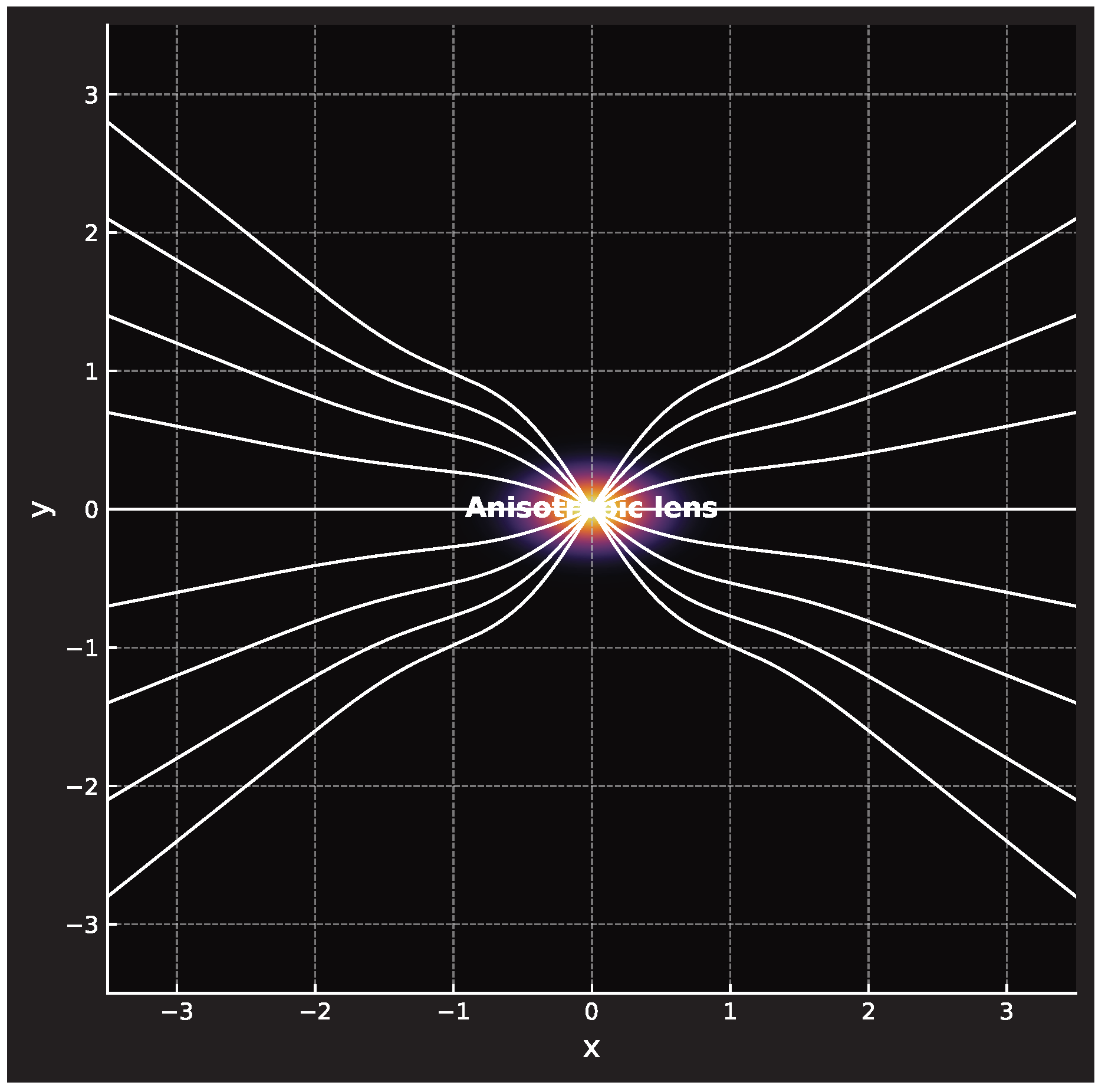
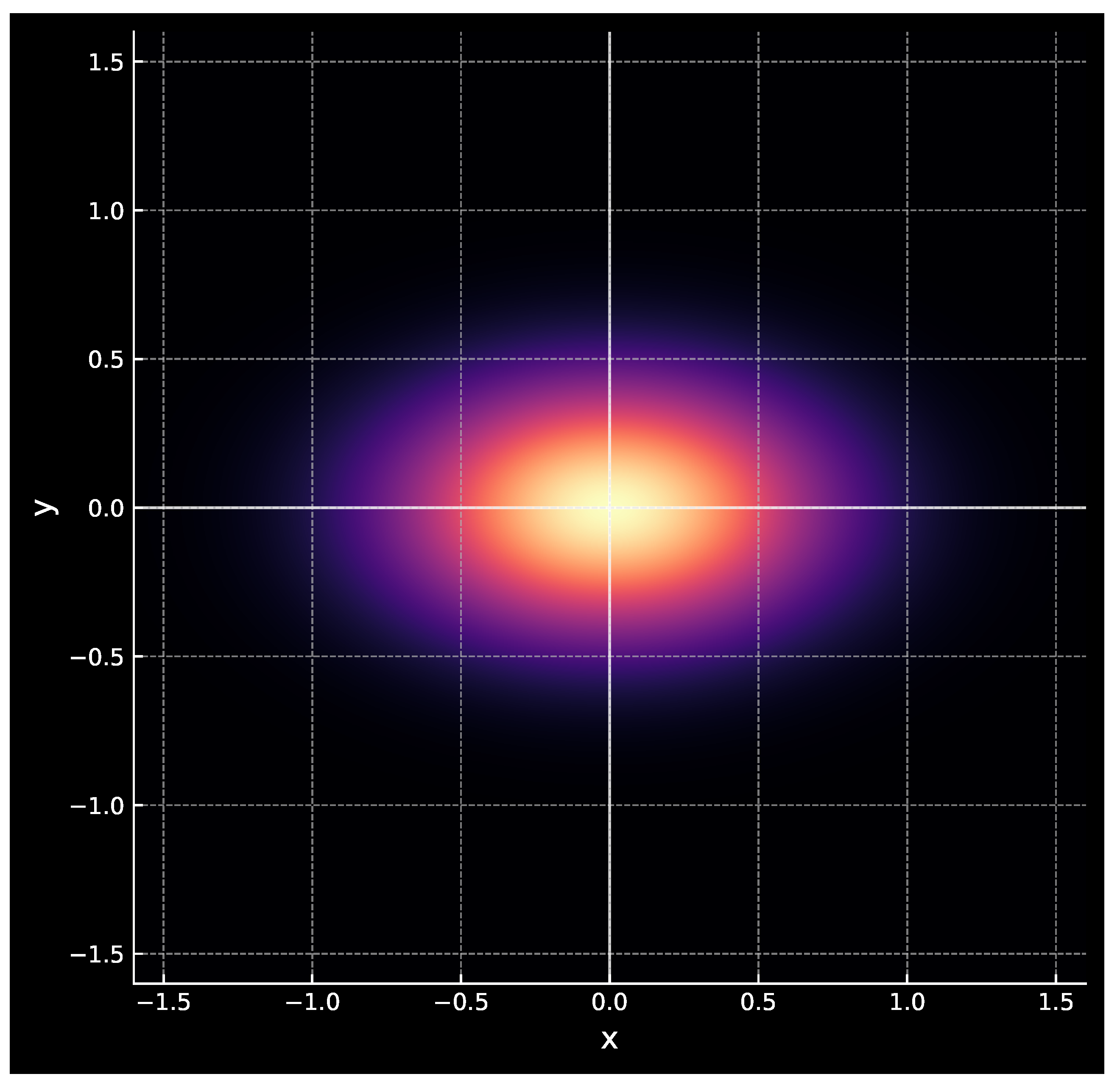
3.11. Anisotropic Regime

Anisotropy of the metric tensor $G_{ik}$ leads to a directional dependence of observables (lensing, propagation of tensor modes, and related effects). Figure 1 schematically illustrates the distribution of anisotropy of the effective Planck scale $L_p(x,\widehat{n})={\ell }_{*}\sqrt{G_{ik}{\widehat{n}}^i{\widehat{n}}^k}$.

4. Cosmology with Geometry–Dependent $L_p$ and $c_{\mathrm{eff}}$

4.1. Setup and Calibration

The fundamental constant ${\ell }_{*}$ is fixed once and for all. However, the local effective Planck length

$$L_p(t,\widehat{n})={\ell }_{*}\sqrt{G_{ik}\left(t\right){\widehat{n}}^i{\widehat{n}}^k}$$

and the corresponding signal speed

$$c_{\mathrm{eff}}\left(t\right)={\left({\displaystyle \frac{\hslash G}{{\left[L_p\left(t\right)\right]}^2}}\right)}^{1/3}$$

may vary with the evolution of the metric tensor $G_{ik}\left(t\right)$. Calibration at the present epoch $t_0$ fixes $L_p\left(t_0\right)={\ell }_p$ and $c_{\mathrm{eff}}\left(t_0\right)=c_0$.

The slow, adiabatic evolution of $G_{ik}\left(t\right)$ ensures that local Lorentz invariance and the causal structure within each neighborhood are preserved at every epoch, while only the large–scale signal cone defined by $c_{\mathrm{eff}}\left(t\right)$ changes in time.

4.2. Modified Friedmann Equations

For a spatially homogeneous and isotropic geometry the line element can be written as

$$d{s}^2=c_{\mathrm{eff}}{\left(t\right)}^{2}d{t}^2-a{\left(t\right)}^{2}d{\mathrm{\Sigma }}_k^2,$$

where $d{\mathrm{\Sigma }}_k^2$ is the metric of constant spatial curvature k. Treating $c_{\mathrm{eff}}\left(t\right)$ as the operational signal speed that sets the causal structure, the Einstein equations take the form

$$\begin{array}{cc}\hfill {\left({\displaystyle \frac{\dot{a}}{a}}\right)}^2& ={\displaystyle \frac{8\pi G}{3}}\rho -{\displaystyle \frac{k{c}_{\mathrm{eff}}{\left(t\right)}^2}{a^2}}+{\displaystyle \frac{\mathrm{\Lambda }{c}_{\mathrm{eff}}{\left(t\right)}^2}{3}},\hfill \end{array}$$

(25)

$$\begin{array}{cc}\hfill {\displaystyle \frac{\ddot{a}}{a}}& =-{\displaystyle \frac{4\pi G}{3}}\left(\rho +{\displaystyle \frac{3p}{c_{\mathrm{eff}}{\left(t\right)}^2}}\right)+{\displaystyle \frac{\mathrm{\Lambda }{c}_{\mathrm{eff}}{\left(t\right)}^2}{3}}.\hfill \end{array}$$

(26)

The operational horizon distance is then

$$d_H\left(t\right)=a\left(t\right){\int }_0^t{\displaystyle \frac{c_{\mathrm{eff}}\left(t^{\prime }\right)}{a\left(t^{\prime }\right)}}d{t}^{\prime },$$

(27)

which measures the maximum comoving separation over which causal contact is possible.

Energy conservation in this framework follows from the covariant identity ${\nabla }_{\mu }{T}^{\mu \nu }=0$, which yields the modified continuity equation

$$\dot{\rho }+3H\left(\rho +{\displaystyle \frac{p}{c_{\mathrm{eff}}^2}}\right)=-\rho {\displaystyle \frac{{\dot{c}}_{\mathrm{eff}}}{c_{\mathrm{eff}}}}.$$

(28)

The right–hand side represents the geometric exchange of energy between matter and the varying causal structure: when $c_{\mathrm{eff}}$ decreases, part of the total energy density is effectively transferred into the background geometry.

If at an early epoch the metric anisotropy causes $L_p\left(t\right)\to 0$ and hence, by Eq. (3), $c_{\mathrm{eff}}\left(t\right)\to \infty$, the integral (27) becomes large even without an inflationary phase, thereby naturally resolving the horizon problem. The same mechanism also regularizes the initial singularity by introducing the finite microscopic scale ${\ell }_{*}$.

4.3. Evolution of $L_p\left(t\right)$ and the Law for $c_{\mathrm{eff}}\left(t\right)$

From Eq. (3) one obtains

$$c_{\mathrm{eff}}\left(t\right)={\left({\displaystyle \frac{\hslash G}{{\left[L_p\left(t\right)\right]}^2}}\right)}^{1/3}=c_0{\left({\displaystyle \frac{L_p\left(t\right)}{L_p\left(t_0\right)}}\right)}^{-2/3}.$$

(29)

Thus, an increase of the effective Planck length $L_p\left(t\right)$ with cosmic time corresponds to a decrease of the effective signal speed $c_{\mathrm{eff}}\left(t\right)$. Because $L_p\left(t\right)$ is determined by the evolving metric component $G_{ik}\left(t\right)$, the apparent variation of $c_{\mathrm{eff}}$ reflects purely geometric evolution rather than any change in the fundamental constants ℏ, G, or ${\ell }_{*}$.

Operationally, $c_{\mathrm{eff}}\left(t\right)$ governs the null–cone for large–scale causal processes (e.g., horizon formation), whereas all local laboratory measurements remain tied to the constant $c_{\mathrm{loc}}$ of the metric (5).

Having established the large–scale consequences of the variable geometric scale, we now turn to its microscopic manifestation—the appearance of stable topological defects that correspond to elementary particles.

5. Elementary Particles as Topological Defects

5.1. General Concept

Elementary particles are interpreted as stable, localized defects of spatial connectivity. Each defect corresponds to a continuous field configuration $A_i\left(x\right)$ whose topology cannot be removed by smooth deformations of the geometry. The associated topological invariants (winding number, linking class, Hopf index) encode the particle’s charge, spin, and baryon number.

5.2. Topological Invariants and Energy Functional

Every finite–energy configuration of the antisymmetric field $A_i$ is characterized by an integer–valued invariant of the form

$$Q_{\mathrm{link}}={\displaystyle \frac{1}{16{\pi }^2}}\int d^{3}x{ϵ}^{ijk}{A}_i{F}_{jk}={\displaystyle \frac{1}{4{\pi }^2}}\int \mathbf{A}·(\nabla \times \mathbf{A})d^{3}x,$$

(30)

which counts the linking of field lines and coincides with the Hopf index H. Here $F_{ij}$ denotes the spatial components of the antisymmetric connectivity tensor introduced in §3.4; in the quasi–isotropic limit $F_{ij}\approx A_{ij}$. Configurations with different $Q_{\mathrm{link}}$ cannot be transformed into each other continuously. The field energy

$$E\left[A_i\right]=\int d^{3}x{\displaystyle \frac{1}{2{\mu }_0}}{F}_{ij}{F}^{ij},$$

(31)

has local minima at fixed $Q_{\mathrm{link}}$, providing topological protection of the defect. This mechanism parallels the stability of solitons in the Faddeev–Niemi and Skyrme models [4,5,6].

5.3. Model Configurations

Stable localized solutions of the energy functional (31) exist for discrete values of the linking number $Q_{\mathrm{link}}$. Below we summarize the lowest–order configurations that correspond to the known elementary fermions.

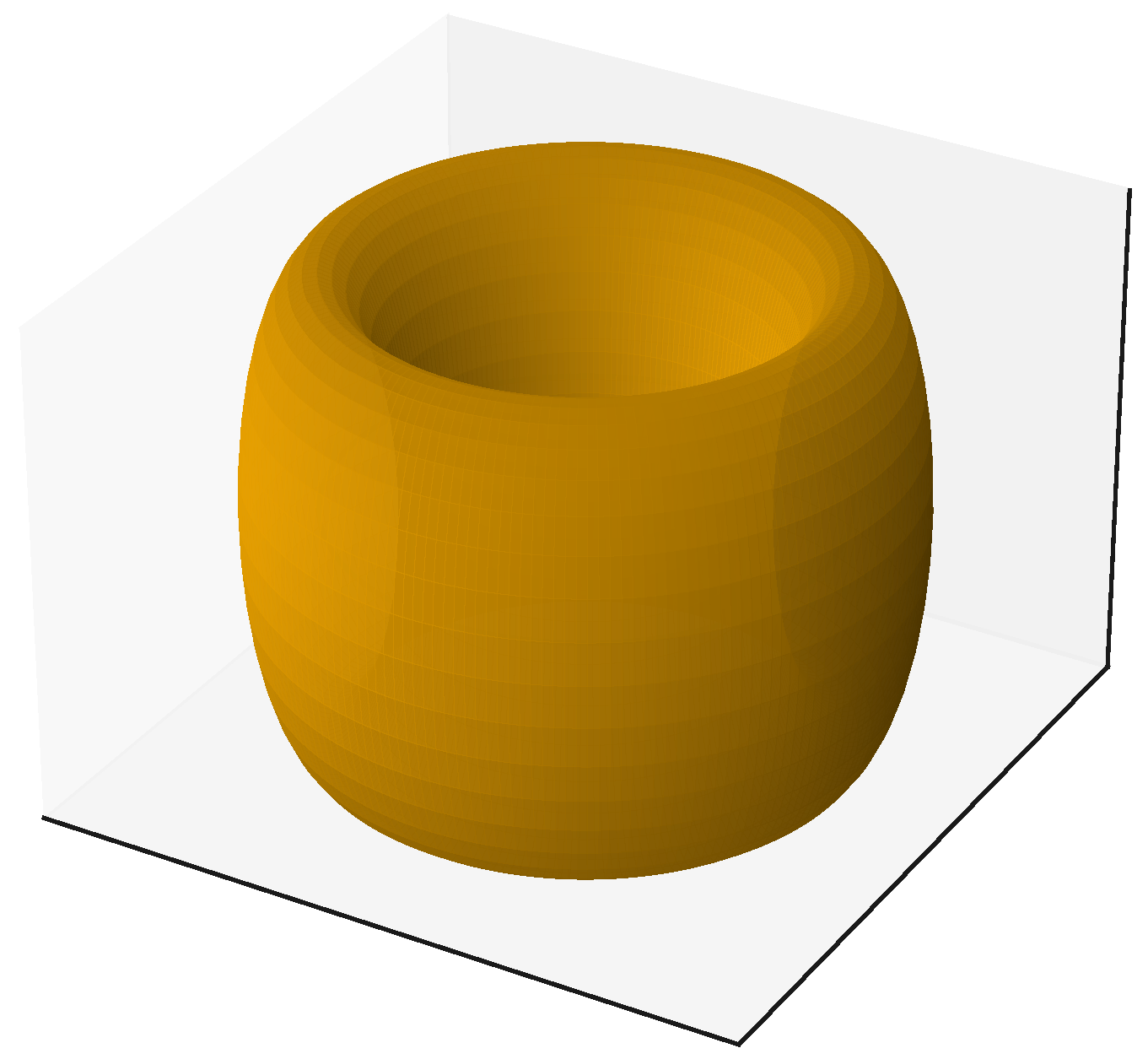
Electron (toroidal defect).

A single–link ($|Q_{\mathrm{link}}|=1$) configuration has toroidal symmetry with a stable circulation of $F_{\mu \nu }$. The electric charge e corresponds to the sign of the linking number, and the spin orientation follows from the direction of circulation. The configuration is single–connected under $2\pi$ rotations and changes sign under a $2\pi$ spatial rotation while returning to itself only after $4\pi$, reproducing the spinor behaviour of a fermion with $s=\frac{1}{2}$.

Figure 2. Model configuration of an electron as a toroidal topological defect with $|Q_{\mathrm{link}}|=1$.

Figure 2. Model configuration of an electron as a toroidal topological defect with $|Q_{\mathrm{link}}|=1$.

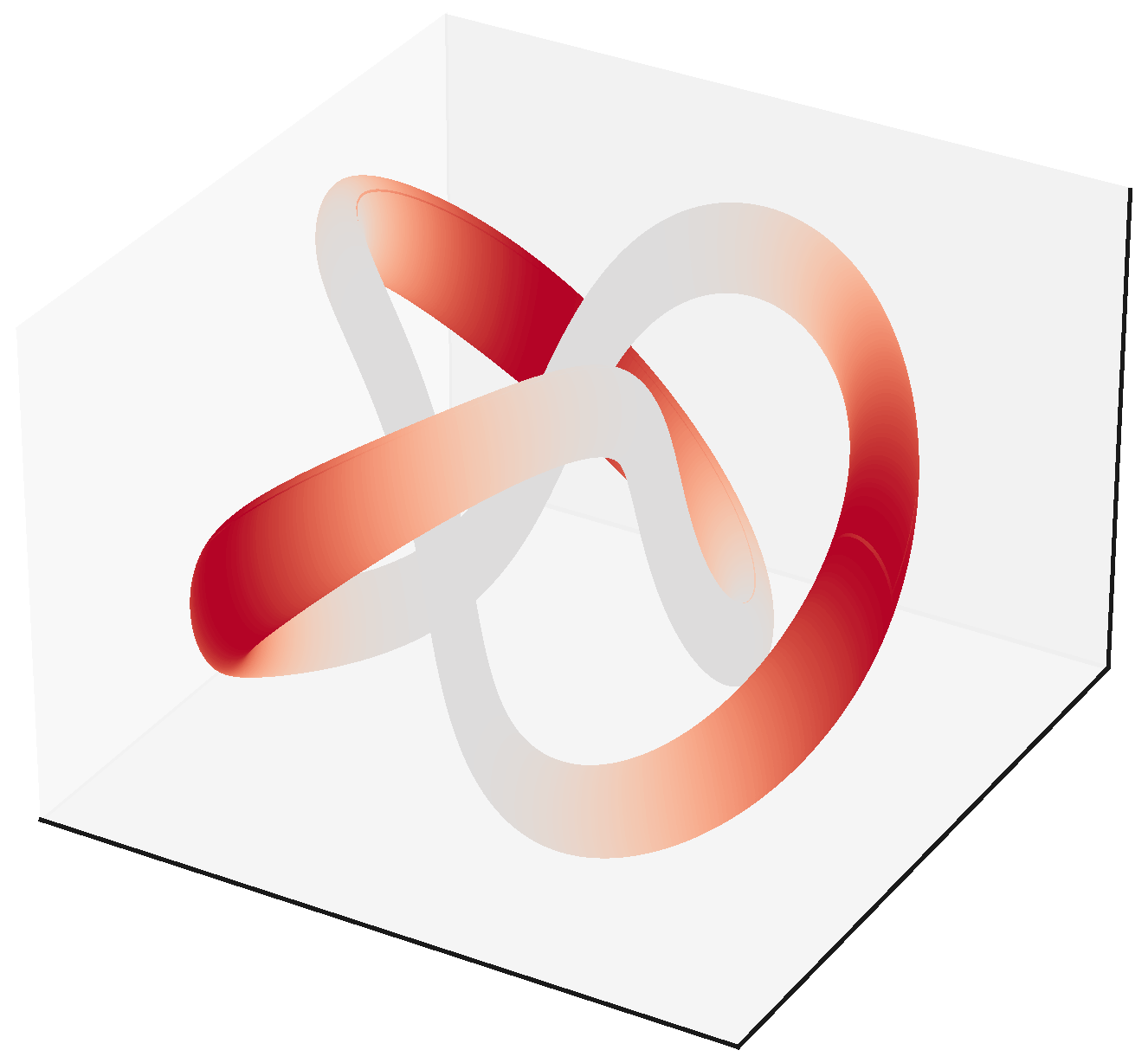
Proton (trefoil–type knot).

A configuration with $|Q_{\mathrm{link}}|=3$ corresponds to a knotted trefoil structure with three intertwined channels of field circulation. These channels naturally parallel the three color degrees of freedom in QCD, while the total orientation of the flows gives net charge $+e$. The trefoil knot belongs to the $C_3$ symmetry class: its three equivalent branches provide a natural geometric analogue of the three $SU{\left(3\right)}_{\mathrm{color}}$ channels in quantum chromodynamics.

Figure 3. Model configuration of a proton as a trefoil–type knot with $|Q_{\mathrm{link}}|=3$.

Figure 3. Model configuration of a proton as a trefoil–type knot with $|Q_{\mathrm{link}}|=3$.

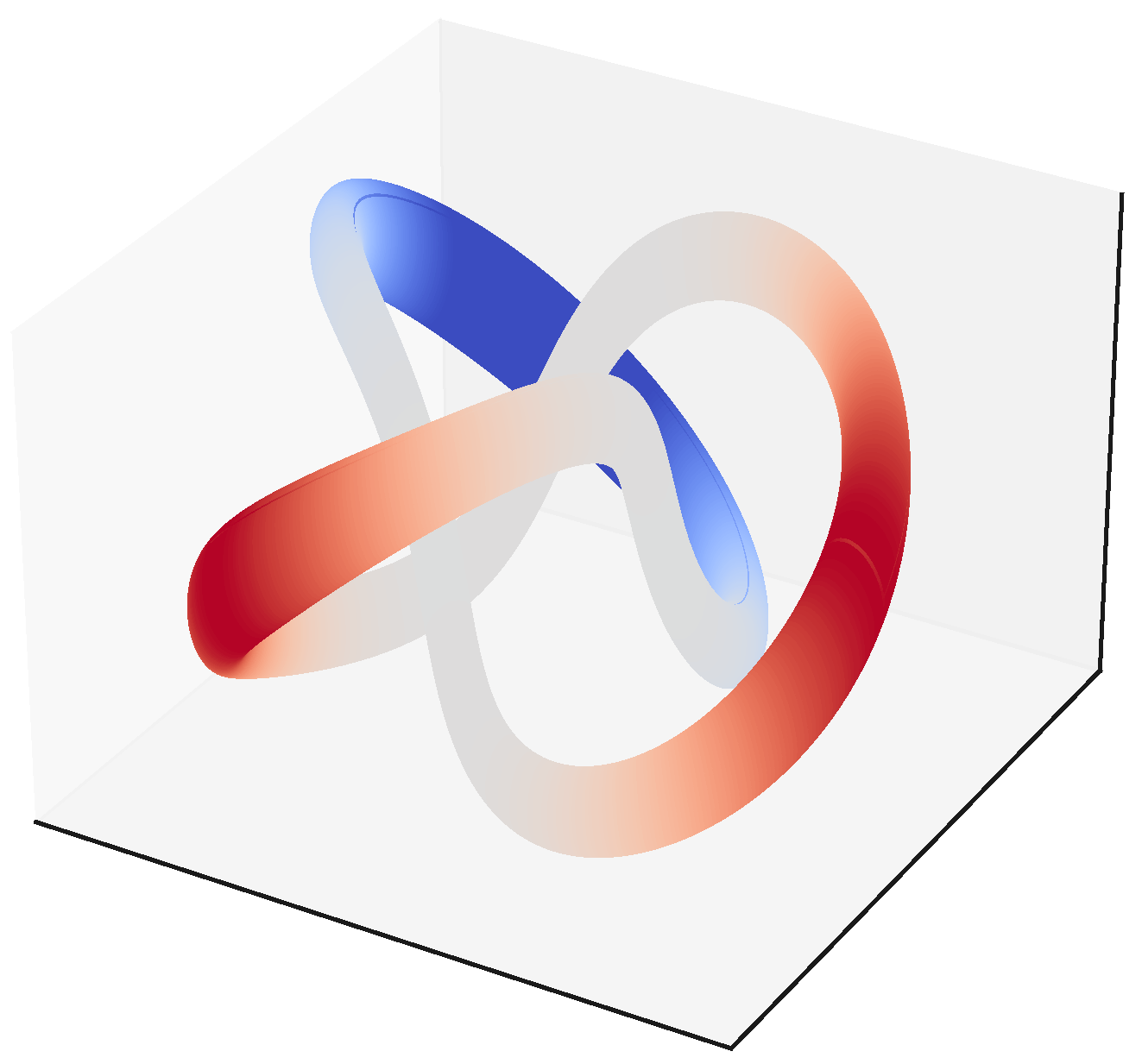
Neutron (balanced knot).

A neutral configuration similar to the proton but with opposite linking in one of the channels, yielding total charge 0. The overall topological class remains the same (${\pi }_3\left(S^3\right)$ invariant conserved), ensuring baryon number conservation, while the internal orientation of one strand is reversed, producing charge neutrality without altering the total spin orientation. Beta decay corresponds to a local reconnection of field lines,

$$n\to p+e^{-}+{\overline{\nu }}_e,$$

which reduces the net linking number by one unit and emits a leptonic filament representing the antineutrino.

Figure 4. Model configuration of a neutron as a balanced neutral knot.

Figure 4. Model configuration of a neutron as a balanced neutral knot.

These configurations form the minimal topological basis of the model; their conserved invariants account for charge, spin, and baryon number, as discussed in the next subsection.

5.4. Physical Properties Derived from Topology

The observable quantum numbers of elementary particles follow directly from the topological invariants of their connectivity configurations. Below we summarize the correspondence between geometric quantities and physical observables.

Charge as winding number.

Electric charge is identified with the integer winding of the $U\left(1\right)$ phase $\varphi$ around a closed loop $\gamma$ in the connectivity domain:

$$Q=ne,{\displaystyle \frac{1}{2\pi }}{\oint }_{\gamma }\nabla \varphi ·d\ell =n\in \mathbb{Z}.$$

(32)

The integer n represents the homotopy class ${\pi }_1\left(S^1\right)$ of the phase map, and the factor e fixes the physical unit of charge by calibration to the electron. Quantization of charge thus follows from the topological quantization of the phase circulation, as in classical soliton models [4,6].

Spin as orientation of circulation.

A toroidal defect admits two stable orientations of phase circulation (clockwise/counter–clockwise). Upon a $2\pi$ spatial rotation the configuration changes sign, while a $4\pi$ rotation restores identity, reproducing the spinor property of fermions ($s=\frac{1}{2}$) [7]. The two orientations correspond to the double covering $SU\left(2\right)\to SO\left(3\right)$ of the rotation group, so that the defect’s phase field lives on a nontrivial spin bundle over ${\mathrm{\Sigma }}_t$.

Stability and mass.

Topological protection ensures stability: a torus or knot cannot be continuously deformed into vacuum without breaking connectivity. The particle mass corresponds to the minimum of the energy functional (31) at fixed $Q_{\mathrm{link}}$. Different topological classes yield different minima, explaining the hierarchy between electron, proton, and neutron masses. The characteristic energy density scales as $E\sim \hslash c_{\mathrm{loc}}/{\ell }_{*}$, so that the rest mass $m\sim E/c_{\mathrm{loc}}^2$ provides a natural link between the geometric cutoff ${\ell }_{*}$ and the observed mass spectrum.

Color and baryon number from knot structure.

Trefoil–type defects possess three intertwined branches, naturally associated with three color channels. The conserved baryon number corresponds to the homotopy invariant ${\pi }_3\left(S^3\right)$ characterizing the knot class, analogous to the Skyrme baryon number [4,6]. The integer associated with ${\pi }_3\left(S^3\right)$ measures the degree of the map from physical space to the compactified field space and remains invariant under smooth deformations, ensuring baryon number conservation.

Beta decay as reconnection.

Neutron decay $n\to p+e^{-}+{\overline{\nu }}_e$ corresponds to a local reconnection that changes $Q_{\mathrm{link}}\mapsto Q_{\mathrm{link}}-1$, reducing the total linking by one unit and emitting a leptonic filament representing the antineutrino. Similar reconnection phenomena are observed in knotted field configurations [8,9,10].

Quantitative estimates.

Experimental bounds on the electron radius $r_e<{10}^{-19}\mathrm{m}$ imply that the toroidal core of the corresponding defect satisfies $r_{\mathrm{core},e}\lesssim {10}^{-19}\mathrm{m}$. For the proton, assuming a core radius $r_{\mathrm{core}}\sim 0.25\mathrm{fm}$ and total trefoil radius $R\sim 0.8\mathrm{fm}$, one obtains an effective charge radius $\sim 0.84\mathrm{fm}$, in agreement with experiment. These values make the model quantitatively falsifiable rather than purely qualitative.

These relations demonstrate that the intrinsic quantum numbers of matter arise from purely geometric invariants of space connectivity, providing a direct bridge between topology and particle phenomenology.

Limitations.

The present correspondence between geometric topology and particle physics remains incomplete. In particular, the chiral structure of weak interactions has not yet been derived explicitly, and anomaly–cancellation conditions are not automatically guaranteed by topology alone. Quantitative predictions such as particle masses, mixing angles, and coupling constants require explicit minimization of the energy functionals for each topological defect. These open issues define natural directions for further development, in line with ongoing studies of topological solitons and knotted field configurations in particle physics.

6. Observable Effects

The framework predicts several potentially observable consequences of metric anisotropy and geometry–dependent effective constants. The most promising channels include gravitational lensing, propagation of gravitational waves, laboratory tests of metric corrections, and cosmological imprints in the early Universe.

Each effect below follows directly from the local anisotropy tensor ${\beta }_{ik}=G_{ik}-{\delta }_{ik}$ and the geometry–dependent signal speed $c_{\mathrm{eff}}\left(x\right)$, providing experimentally accessible constraints on the underlying geometry.

6.1. Anisotropic Lensing

A directional dependence of the deflection angle in weak fields arises from the anisotropy of the spatial metric $G_{ik}={\delta }_{ik}+{\beta }_{ik}$, where $\mathrm{tr}\beta =0$. The effective gravitational potential satisfies the Poisson equation ${\nabla }^2{\mathrm{\Phi }}_{\mathrm{eff}}=4\pi G\rho (1+{\beta }_{ij}{\widehat{n}}^i{\widehat{n}}^j)$, so that the effective mass becomes angle–dependent, $M_{\mathrm{eff}}\left(\phi \right)$. To first order in ${\beta }_{ik}$,

$$\widehat{\alpha }\left(\phi \right)\simeq {\displaystyle \frac{4G{M}_{\mathrm{eff}}\left(\phi \right)}{c_{\mathrm{eff}}^{2}b}}\left[1+\frac{1}{2}{\beta }_{ij}{\widehat{n}}^i{\widehat{n}}^j\right],$$

(33)

where b is the impact parameter. Observation of direction–dependent deflection would therefore probe the anisotropic components of $G_{ik}$. For typical weak–lensing angles $\widehat{\alpha }\sim {10}^{-5}$, an anisotropy $\left|\beta \right|\sim {10}^{-3}$ would produce a differential deflection $\Delta \widehat{\alpha }\sim {10}^{-8}$ rad, within reach of next–generation surveys (Euclid, SKA).

Figure 5. Schematic illustration of anisotropic lensing due to geometric anisotropy of the metric $G_{ik}$.

Figure 5. Schematic illustration of anisotropic lensing due to geometric anisotropy of the metric $G_{ik}$.

6.2. Speed of Gravitational Waves

The effective metric for tensor modes may produce a mild directional dependence of the phase velocity:

$$v_g\left(\widehat{\mathbf{n}}\right)\approx c_{\mathrm{eff}}[1+\delta \left(\widehat{\mathbf{n}}\right)],\left|\delta \right|\ll 1,$$

(34)

where $\delta \left(\widehat{\mathbf{n}}\right)\simeq \frac{1}{2}{\beta }_{ij}{\widehat{n}}^i{\widehat{n}}^j$ at leading order. The observational bound $|v_g-c_{\mathrm{eff}}|/c_{\mathrm{eff}}\lesssim {10}^{-15}$ from GW170817 translates into a constraint on the anisotropy amplitude $|{\beta }_{ik}|\lesssim {10}^{-15}$, confirming that local Lorentz invariance holds with extremely high precision. Future multi–messenger detections with LISA and pulsar–timing arrays could improve this limit by several orders of magnitude.

6.3. Laboratory Tests

Strong electromagnetic fields can induce minute corrections to the metric via the field stress tensor (17). For a uniform field region, the fractional correction to the metric can be estimated as

$${\displaystyle \frac{\delta g}{g}}\sim {\displaystyle \frac{E^2+B^2}{E_{\mathrm{Planck}}^2}},E_{\mathrm{Planck}}\equiv {\displaystyle \frac{c_{\mathrm{loc}}^4}{\sqrt{G}}}\approx 1.3\times {10}^{61}\mathrm{V}/\mathrm{m},$$

(35)

which is exceedingly small ($\sim {10}^{-40}$ for laboratory fields with $E,B\sim {10}^9\mathrm{V}/\mathrm{m}$) but may in principle be enhanced in resonant optical cavities, high–intensity laser systems, or precision interferometric setups where cumulative phase shifts scale with optical path length. A null result at the level of $\delta g/g<{10}^{-35}$ would already constrain ${\ell }_{*}$ to be below $\sim {10}^{-23}\mathrm{m}$.

6.4. Cosmological Signatures

Temporal variation of the geometry–dependent quantities $L_p\left(t\right)$ and $c_{\mathrm{eff}}\left(t\right)$ modifies the sound horizon and the growth of super–horizon correlations in the early Universe. Observable consequences include slight shifts in the positions of the acoustic peaks in the CMB spectrum and potential distortions in the stochastic gravitational–wave background, both of which provide quantitative tests of the model. To first order, the fractional shift of the sound horizon obeys

$${\displaystyle \frac{\Delta r_s}{r_s}}\simeq -{\displaystyle \frac{2}{3}}{\displaystyle \frac{\Delta c_{\mathrm{eff}}}{c_{\mathrm{eff}}}}\approx -{\displaystyle \frac{2}{3}}{\displaystyle \frac{\Delta L_p}{L_p}},$$

(36)

implying that a ${10}^{-3}$ change in $L_p$ during recombination would shift the first acoustic peak by $\Delta \ell \sim 1$, a level detectable with current CMB precision. Similarly, slow temporal drifts of $c_{\mathrm{eff}}\left(t\right)$ alter the transfer function of primordial tensor modes, producing frequency–dependent tilts in the stochastic gravitational–wave background that could be probed by LISA and PTA networks.

Together, these effects translate the purely geometric parameters $({\ell }_{*},G_{ik})$ into observable quantities across a wide range of scales, from tabletop optics to cosmology, offering a falsifiable phenomenology for the unified connectivity framework.

7. Comparison with Current Topological Theories

To place the proposed framework in context, we compare it with the main existing topological and quantum–geometric approaches. The emphasis is on the number of fundamental parameters, the mathematical carriers of topology, and the type of observable predictions.

7.1. Cosmic Defects

The classical Kibble mechanism and the models of Vilenkin and Shellard [11,12] describe the formation of domain walls, strings, and monopoles during phase transitions in the early Universe. Recent PTA results (NANOGrav, EPTA, PPTA) indicate a stochastic gravitational–wave background [13], potentially explainable by cosmic strings [14,15]. In contrast, the present framework treats the defect as the connectivity geometry itself, governed by a single fundamental scale ${\ell }_{*}$. An observational discriminator would be the angular anisotropy of the SGWB in the case of an anisotropic spatial metric $G_{ik}$. The predicted pattern of multipoles depends on the tensor ${\beta }_{ik}$ and may be constrained by future PTA anisotropy measurements.

7.2. Hopfions and Knotted Electromagnetic Fields

Works by Ranada [8], Irvine and Kedia [9], and subsequent reviews [10] demonstrate that Maxwell’s equations admit knotted and linked field configurations (“hopfions”) classified by the Hopf index H. In the present model, similar topological structures arise at the level of spatial connectivity rather than within a separate material field. Nevertheless, the same computational tools for evaluating H apply to our particle–like defects (electron, proton, neutron), enabling quantitative analysis of their stability and energy hierarchy. The geometric cutoff ${\ell }_{*}$ plays the role of a natural ultraviolet regulator that replaces the arbitrary core size used in standard hopfion simulations.

7.3. Skyrme Model of Baryons

The Skyrme model [4] and its modern extensions [16,17] describe baryons as topological solitons in nonlinear $\mathrm{SU}\left(2\right)$ fields, where the baryon number corresponds to a ${\pi }_3\left(S^3\right)$ invariant. In our framework the carrier of topology is the three–dimensional connectivity itself, and the single parameter ${\ell }_{*}$ defines the geometric cutoff scale. This removes the arbitrariness of choosing a specific Lagrangian and facilitates direct comparison with observable quantities such as proton and neutron radii. While Skyrme models contain multiple phenomenological constants ($f_{\pi }$, $e_{\mathrm{Sk}}$, …), the present construction uses only one universal length ${\ell }_{*}$, reducing parameter degeneracy while preserving the same topological content.

7.4. Loop Quantum Gravity and Kerr Regularization

Recent results within loop quantum gravity (LQG) [18,19] demonstrate the removal of the Kerr ring singularity and the emergence of a minimal radius. The present model shares similar phenomenology—absence of closed timelike curves, finite $r_{min}$, and shifts of the ergosphere observable via EHT shadows and GW ringdown spectra. The key distinction is conceptual: in LQG regularization arises from quantization of geometry with several free parameters (e.g. Barbero–Immirzi $\gamma$), whereas here it stems from a single geometric–topological scale ${\ell }_{*}$. This difference yields distinct deformation portraits of the Kerr metric, which can be tested by Bayesian fits to EHT and LIGO/Virgo/KAGRA data. Quantitatively, the expected shift of the photon–ring radius is $\Delta r/r\simeq {({\ell }_{*}^2/R_S^2)}^{1/3}$, yielding $\Delta r/r\sim {10}^{-3}$ for ${\ell }_{*}\sim {10}^{-22}\mathrm{m}$ and a $10M_{\odot }$ black hole—within the reach of next–generation EHT baselines.

7.5. Astrophysical Tests of Kerr

Observations of the M87* and Sgr A* shadows (EHT [20,21]) and of gravitational–wave ringdown spectra (LIGO/Virgo/KAGRA [22]) already provide direct probes of regularized Kerr geometries. Moreover, the constraint on the speed of gravitational waves from GW170817 [23] requires $|c_{\mathrm{gw}}-c|/c\lesssim {10}^{-15}$, which the present model satisfies automatically since local Lorentz invariance with fixed $c_{\mathrm{loc}}$ is preserved by construction.

Summary of distinctions.

Framework	Carrier of topology	Free parameters	Singularities	Observable tests
GR + EM	metric $g_{\mu \nu }$ + field $A_{\mu }$	none	yes	lensing, GW speed
Cosmic strings	scalar/gauge fields	tension $\mu$	yes	SGWB anisotropy
Skyrme model	$SU\left(2\right)$ field $U\left(x\right)$	$f_{\pi },e_{\mathrm{Sk}}$	regular	baryon masses
LQG	spin networks	$\gamma$, etc.	regular	BH area spectrum
This work	connectivity tensor $G_{ik}$	${\ell }_{*}$	regular	CMB, EHT, PTA

The comparison shows that the proposed theory retains the minimal set of assumptions while covering both the microscopic (particle) and macroscopic (cosmological and gravitational) domains. Its falsifiability through direct astronomical and laboratory tests distinguishes it from most existing topological approaches.

8. Discussion and Outlook

The proposed axiomatic framework unifies the geometric description of gravity and electromagnetism through the concept of local spatial connectivity. Within this picture, both curvature and field strength originate from a single tensor $G_{ik}$, whose symmetric and antisymmetric components represent, respectively, gravitational and electromagnetic sectors. The introduction of one universal scale ${\ell }_{*}$ regularizes classical singularities and provides a geometric origin for quantum phenomena. Future work will refine the operational definition of ${\ell }_{*}$, extend the classification of topological defects, and provide numerical modeling of the evolution of $L_p\left(t\right)$ with confrontation to astrophysical and cosmological data.

Phenomenological constraints.

Precision measurements of the electron $g-2$ and electric dipole moment require any internal structure to appear only above a compositeness scale $\mathrm{\Lambda }\gtrsim {10}^{20}{\mathrm{m}}^{-1}\sim 10\mathrm{TeV}$. The present construction is consistent with these limits, since the characteristic core size of the electron defect is expected to satisfy $r_{\mathrm{core},e}\ll {\mathrm{\Lambda }}^{-1}\sim {10}^{-20}\mathrm{m}$. Astrophysical tests from EHT shadows and gravitational–wave ringdown spectra further restrict the geometric scale to ${\ell }_{*}\lesssim {10}^{-22}$–${10}^{-23}\mathrm{m}$, consistent with the absence of measurable deviations from general relativity.

Future directions.

Promising extensions of the framework include:

(i)

numerical minimization of toroidal and knotted configurations to estimate corresponding particle masses and magnetic moments;

(ii)

explicit treatment of chirality and weak interactions within the connectivity picture;

(iii)

confrontation with observational signatures such as particle charge radii, anisotropic gravitational lensing by macroscopic defects, and the angular structure of the SGWB;

(iv)

exploration of links with quantum–information geometry and Fisher–based formulations of quantum mechanics, which may provide an alternative derivation of the quantum potential at the scale ${\ell }_{*}$;

(v)

development of an effective Lagrangian for $G_{ik}$ to connect the present axiomatic model with covariant field theory.

Concluding remark.

Overall, the theory provides a unified geometric language linking gravity, electromagnetism, and quantum structure, while remaining directly testable through cosmological and astrophysical observations. By reducing the number of postulates to a single fundamental scale ${\ell }_{*}$, it opens a route toward a falsifiable and minimal unification scheme where topology, geometry, and dynamics emerge from one underlying principle.

References

- Polchinski, J. String Theory. Vols. 1–2; Cambridge University Press, 1998.
- Rovelli, C. Quantum Gravity; Cambridge University Press, 2004.
- Ashtekar, A.; Lewandowski, J. Background Independent Quantum Gravity: A Status Report. Classical and Quantum Gravity 2004, 21, R53–R152, [gr-qc/0404018]. [CrossRef]
- Skyrme, T.H.R. A Non-Linear Field Theory. Proceedings of the Royal Society A 1961, 260, 127–138. [CrossRef]
- Faddeev, L.D.; Niemi, A.J. Stable knot-like structures in classical field theory. Nature 1997, 387, 58–61. [CrossRef]
- Manton, N.; Sutcliffe, P. Topological Solitons; Cambridge University Press, 2004. [CrossRef]
- Wilczek, F.; Zee, A. Linking Numbers, Spin, and Statistics of Solitons. Physical Review Letters 1983, 51, 2250–2252. [CrossRef]
- Rañada, A.F. A Topological Theory of the Electromagnetic Field. Letters in Mathematical Physics 1989, 18, 97–106. [CrossRef]
- Kedia, H.; Bialynicki-Birula, I.; Peralta-Salas, D.; Irvine, W.T.M. Tying Knots in Light Fields. Physical Review Letters 2013, 111, 150404, [1302.0342]. [CrossRef]
- Guslienko, K.Y. Magnetic Hopfions: A Review. Magnetism 2024, 4, 383–399. [CrossRef]
- Kibble, T.W.B. Topology of Cosmic Domains and Strings. Journal of Physics A: Mathematical and General 1976, 9, 1387–1398. [CrossRef]
- Vilenkin, A.; Shellard, E.P.S. Cosmic Strings and Other Topological Defects; Cambridge University Press, 1994.
- Agazie, G.; et al. The NANOGrav 15-year Data Set: Evidence for a Gravitational-Wave Background. The Astrophysical Journal Letters 2023, 951, L8, [2306.16213]. [CrossRef]
- Auclair, P.; Ringeval, C.; Sakellariadou, M.; Steer, D.A. Probing the gravitational wave background from cosmic strings with LISA. Journal of Cosmology and Astroparticle Physics 2019, 2019, 030, [1909.00819]. [CrossRef]
- LISA Consortium. Laser Interferometer Space Antenna: Science Requirements and Mission Status, 2024.
- Beznogov, M.V.; Raduta, A.R. Bayesian Survey of the Dense Matter Equation of State built upon Skyrme effective interactions, 2023, [2308.15351]. arXiv preprint.
- Beznogov, M.V.; Raduta, A.R. Bayesian inference of the dense matter equation of state built upon extended Skyrme interactions. arXiv preprint 2024, [2403.19325].
- Fazzini, F.; Husain, V.; Wilson-Ewing, E. Shell-crossings and shock formation during gravitational collapse in effective loop quantum gravity. Physical Review D 2024, 109, 084032, [2312.02032]. [CrossRef]
- Fazzini, F. Non-uniqueness of the shockwave dynamics in effective loop quantum gravity. arXiv preprint 2025, [2502.03003].
- Event Horizon Telescope Collaboration. First M87 Event Horizon Telescope Results. I. The Shadow of the Supermassive Black Hole. The Astrophysical Journal Letters 2019, 875, L1. [CrossRef]
- Event Horizon Telescope Collaboration. First Sagittarius A* Event Horizon Telescope Results. I. The Shadow of the Supermassive Black Hole in the Center of the Milky Way. The Astrophysical Journal Letters 2022, 930, L12. [CrossRef]
- LIGO Scientific Collaboration and Virgo Collaboration and KAGRA Collaboration. Tests of General Relativity with GWTC-3 and implications for ringdown spectroscopy. Physical Review D 2022, 106, 104042. [CrossRef]
- Abbott, B.P.; et al. Gravitational Waves and Gamma-Rays from a Binary Neutron Star Merger: GW170817 and GRB 170817A. The Astrophysical Journal Letters 2017, 848, L13. [CrossRef]