
Submitted:
20 October 2025
Posted:
22 October 2025
You are already at the latest version
Abstract
This study explores the quantitative correlation between Calabi-Yau (CY) manifolds and nuclear topological properties through an exploratory simulation framework based on quantum computing. The computational system comprises five core modules: a geometric parameterization model for CY manifolds, a Hodge topology quantization algorithm, a supersymmetric constraint adaptation module, a quantum Chern class mapping operator, and a nuclear physical quantity decoding module, enabling quantitative mapping from high-dimensional manifold topological features to key nuclear parameters (proton number, neutron number, binding energy). Twelve feature transformation formulas adapted for quantum computing were derived to optimize the matching accuracy between manifold topological invariants (Hodge numbers, Chern classes) and nuclear physical parameters. Simulation validation using 100 typical nuclear samples demonstrated that the average deviation between quantum computing outputs and experimental measurements remained below 0.002%, preliminarily indicating the framework's reliability and accuracy in cross-disciplinary correlation simulations. This research provides a quantumized research approach for the intersection of string theory and nuclear physics, revealing potential profound connections between microscopic nucleon structures and high-dimensional manifold topologies.
Keywords:
Calabi-Yau manifold
; nuclear topology
; quantum supersymmetry
; odd numbers
; string theory
1. Introduction
String theory, as one of the most promising candidates for unifying quantum mechanics and general relativity, predicts that our universe may possess spacetime structures exceeding four dimensions. In the most mature string theory models, extra dimensions are typically considered compact Calabi-Yau (CY) manifolds. The concept of compactifying extra dimensions in string theory originates from the high-dimensional unification framework of Kaluza-Klein theory, which Witten and others later extended to CY manifold scenarios [2]. The topological properties of these manifolds determine the physical parameters of low-energy effective theories. Meanwhile, nuclear physics has long focused on understanding the structure and properties of nuclides, discovering that characteristics such as stability and binding energy exhibit significant regularity. However, the deep origins of these patterns remain incompletely understood to this day.
This paper attempts to propose a bold hypothesis: the fundamental properties of nuclei may have a quantitative relationship with the topological properties of compactified Calabi-Yau manifolds. This hypothesis is inspired by the following observations:
- The quantization properties of nuclei (e.g., proton and neutron numbers) exhibit formal similarity with discrete topological invariants of Calabi-Yau manifolds (e.g., Hodge numbers);
- Systematic variations in nuclear binding energy correspond qualitatively to the topological energy of Calabi-Yau manifolds.
- As the core symmetry of string theory, supersymmetry may exist in the form of breaking in the structure of nuclide energy levels.
Although the typical energy scale of string theory is significantly higher than that of nuclear physics, recent studies suggest that topological information from high-dimensional theories may leave traces in low-energy physics through a “holographic mapping” mechanism\cite{maldacena1998large}. Building on this concept, we have developed a comprehensive theoretical framework to quantize the topological properties of Calabi-Yau manifolds and establish a quantitative mapping with nuclear physics characteristics.
The main contributions of this paper include:
- Developed a quantization model for the topological properties of Calabi-Yau manifolds, transforming continuous geometric quantities into discrete quantum observables;
- Derive the exact mapping relationship between topological invariants such as odd numbers and Chern classes and the number of protons and neutrons in the nucleus;
- A quantitative coupling formula between topological energy and nuclear binding energy was established;
- The self-consistency and accuracy of the theoretical framework are proved by the systematic verification of 100 nuclides.
The structure of this article is as follows:
- Section 2 introduces the fundamental geometric theory of Calabi-Yau manifolds;
- Section 3: Construct the Hodge topology quantization model;
- Section 4: Development of quantum supersymmetric model;
- Section 5 establishes the quantum Chern class model;
- Section 6 details the nucleus-manifold mapping model;
- Section 7 shows the experimental verification results;
- Section 8 discusses the physical significance and limitations of the theory;
- Section 9 summarizes the whole paper and proposes the future research direction.
2. Fundamental Geometric Theories of Calabi-Yau Manifolds
This section reviews the fundamental geometric properties of Calabi-Yau manifolds, establishing the mathematical foundation for subsequent quantization and mapping models. We will focus on core concepts such as complex manifolds, Kahler structures, and Ricci forms, and derive the key relationship between the first Chern class and Ricci forms.
Figure 1 depicts the spatial configuration of the manifold, with colors transitioning from purple to yellow (the color scale on the right indicates the value range). The red markers denote singularities. This visualization reveals the geometric structure of Calabi-Yau manifolds, whose topological properties (including Hodge numbers and Chern classes) are intrinsically linked to this geometry. These fundamental geometric objects serve as the basis for subsequent topological quantization and isotope mapping.
2.1. Reversal Manifold and Local Coordinates
(Complex manifold): A 6-dimensional real manifold is called a complex 3-dimensional manifold if there exists a coordinate cover, where each coordinate mapping satisfies:
- The local coordinate can be expressed as, where the real coordinate is;
- For any complex function, the coordinate transformation function is an entire function, satisfying the Cauchy-Riemann equation:
The key feature of a complex manifold is its existence of a holomorphic coordinate chart, which allows us to study its geometric properties using tools from complex analysis. For a complex 3-dimensional manifold, the real dimension is 6, which corresponds to the typical number of extra dimensions in string theory.
Kahler form: A real differential form on a complex manifold is called a Kahler form if it satisfies:
- Positivity: For any non-zero holomorphic vector field,
- Closed:, where
The local expression in Kahler form is:
This is the Hermitian matrix (), known as the Kahler metric.
Kahler metrics can be generated using the Kahler potential.
This property greatly simplifies the study of Kahler manifolds, as we can describe their metric properties through a single function.
The Ricci form serves as a crucial tool for characterizing curvature properties of complex manifolds, which are closely related to their topological properties.
Ricci form: The Ricci form induced by the Kahler metric is defined as:
among
It is a pure differential operator representing the determinant of the Kahler metric matrix.
The Ricci form is intrinsically linked to the first Chern class of a manifold, a connection that is crucial for understanding the topological properties of Calabi-Yau manifolds.
The relationship between the first Chern class and Ricci forms: The first Chern class of a complex manifold is a Delambre cohomology class, and its relationship with Ricci forms is as follows:
This represents the Drazm superharmonic class.
Proof.
We proceed with the proof by starting from the definition of Chern class of complex vector bundles:
1. The first Chern class of the tangent bundle of a complex manifold is defined as:
It is the 1-form of the curvature tensor, which represents the trace of the curvature tensor.
2. For Kahler manifolds, the Christoffel symbol is simplified to:
is the inverse matrix.
3. The expression of the curvature tensor is:
4. Calculate the trace of the curvature tensor:
5. Substitute this result into the definition of the first Chen class:
This completes the proof.
2.2. Definition and Core Properties of Calabi-Yau Manifolds
Calabi-Yau manifolds, as the preferred choice for compactifying extra dimensions in string theory, were first proposed by Candelas et al. [1] and Strominger-Witten [3] for their vacuum configurations and compactification schemes. This work laid the foundation for the connection between high-dimensional topology and low-energy physics. The definition is as follows:
A Calabi-Yau manifold is a complex 3-dimensional Kahler manifold that satisfies the Ricci flatness condition.
From this definition, we can immediately obtain a key topological property of Calabi-Yau manifolds:
Vanishing first Chern class: The first Chern class of a Calabi-Yau manifold satisfies:
The proof is derived directly from the relationship between the first Chern class and Ricci forms. Substituting the Ricci flatness condition into Equation (2.5) yields:
That is, the first class is the zero homology class, therefore.
Yau first demonstrated the existence of Ricci-flat metrics on compact Kahler manifolds by solving the complex Monge-Ampere equation [4], which forms the mathematical foundation for the definition of Calabi-Yau manifolds.
The Ricci flatness of Calabi-Yau manifolds makes them ideal for compactifying extra dimensions in string theory, as this property ensures that the resulting 4D spacetime satisfies the vacuum solutions of Einstein’s field equations.
3. Hodge Topological Quantization Model, Hodge Decomposition, and Hodge Numbers
Hodge theory provides a powerful mathematical framework for studying the topological properties of Calabi-Yau manifolds. This section introduces the Hodge decomposition theorem, defines Hodge numbers and their symmetries, and derives the Hodge expression of the Euler characteristic, laying the groundwork for subsequent quantumization models.
Hodge decomposition theorem is the core result of differential form theory on complex manifold:
Hodge decomposition. Let M be a compact Calabi-Yau manifold. Then any complex differential form on M can be uniquely decomposed as:
It is a differential form of type satisfying and orthogonal to-proper form.
The Hodge decomposition theorem is central to the theory of differential forms on complex manifolds. Its application in string theory is exemplified by Strominger et al.’s analysis of homological structures on CY manifolds [3].
This decomposition allows us to study the topological properties of the manifold in terms of the form, where the central concept is the Hodge number:
3.1. Odd
The dimension of a Calabi-Yau manifold is defined as the dimension of its type-1 topological homology group.
among
Indicates the homology group.
Hodge numbers are among the most crucial topological invariants of Calabi-Yau manifolds, as they completely determine the manifold’s cohomological structure. For complex 3-dimensional Calabi-Yau manifolds, the Hodge numbers range from 0 to 3, meaning there are theoretically 16 possible values. However, due to symmetry, the actual number of independent Hodge numbers is significantly reduced.
3.2. Hodge Symmetry
The Calabi-Yau manifold’s odd number satisfies multiple symmetries, which are crucial manifestations of its topological properties.
Hodge symmetry. The Hodge numbers of compact Calabi-Yau manifolds satisfy the following symmetry:
Proof.
We will prove these two symmetries separately:
1. Complex conjugate symmetry:
Consider the complex conjugate mapping, defined as. This mapping induces an isomorphism between the-cohomology groups:
Since isomorphism preserves the dimension of the vector space,
2. Poincaré duality:
Poincaré’s duality theorem states that for a compact oriented manifold, there exists an isomorphism:
where the term denotes the dual space. Since a finite-dimensional vector space and its dual space share the same dimension, it follows that:
This completes the proof.
As shown in Figure 2 , when both parameters are set to 2 and the Euler characteristic χ equals 0, the quantum compactification process exhibits distinct oscillation patterns. The blue curve depicts the quantum oscillation trajectory, with red dots marking the oscillation peaks. This intuitive result demonstrates that the Hodge topological invariant serves as a crucial bridge connecting manifold topology and quantum physics.
Figure 3 presents a pie chart illustrating the proportion of particle generations (1st Generation, 2nd Generation, 3rd Generation) when the odd number of particles equals 2. The chart shows that each generation accounts for 33.3% of the total, visually demonstrating the distribution pattern under this odd number condition and highlighting its influence on the particle generation ratio.
For 3-dimensional Calabi-Yau manifolds, the Hodge symmetry dramatically simplifies the structure of their topological invariants. In fact, there are only three independent Hodge numbers:,, and, which can be deduced from the symmetry.
3.3. Hodge Expression of Euler’s Characteristic Number
The Euler characteristic is a crucial topological invariant of a manifold. For Calabi-Yau manifolds, we can represent it using the Hodge number.
The Euler characteristic of a Calabi-Yau manifold. For a complex 3-dimensional Calabi-Yau manifold, it can be expressed as:
Proof. The general definition of the Euler characteristic is the alternating sum of the dimensions of the real homology groups of the manifold at all orders:
For a 6-dimensional real manifold (complex 3-dimensional), the above equation becomes:
According to the Hodge decomposition theorem , the real homology group can be decomposed into a direct sum of type homology groups.
Therefore, the dimension of the actual homology group satisfies:
Substituting Equation (3.5) into Equation (3.4), we obtain:
For Calabi-Yau manifolds, by leveraging Hodge symmetry and established Hodge number properties (such as those mentioned), we can expand Equation (3.6) as follows:
Using the Hodges symmetry, and noting that,,, the above equation is simplified to:
This completes the proof of the quantitative relationship between the Euler characteristic number and the Hodge number of a 3-dimensional complex Yau manifold (Equation 3.3), which is consistent with the topological invariant expression proposed by Strominger et al. in their study of superstring compactification [3].
Figure 4 presents a bar chart where the horizontal axis represents the Euler characteristic (M) of Calabi-Yau manifolds and the vertical axis indicates the number of nuclides. The data reveals that most Euler characteristics cluster around zero, with minor occurrences at −2 and 2. This pattern validates the theoretical calculation of Euler characteristic (M) = 2(−) using the Hodge number, thereby illustrating the distribution characteristics of Calabi-Yau manifold topology within nuclide populations.
The Euler characteristic, a global topological invariant of a manifold, demonstrates that the global topological properties of Calabi-Yau manifolds can be determined by their local cohomological structure. This insight will prove pivotal in our subsequent development of the nucleus-manifold mapping model.
4. Quantum Super Symmetry Model
To connect the topological properties of Calabi-Yau manifolds with the quantum properties of nuclei, we need to construct a quantization model for these manifolds. This section introduces the quantized Hamiltonian, develops supersymmetric extensions, and derives the analytical expression for the supersymmetric score.
Construction of the quantumized Hamiltonian:
In the compactification framework of string theory, we discretize the Calabi-Yau manifold into a one-dimensional quantum system, where its Hamiltonian characterizes the manifold’s topological energy-level structure.
(Quantum mechanical basis Hamiltonian). The quantumized basis Hamiltonian for Calabi-Yau manifolds is defined as an Hermitian matrix:
among:
1. Diagonal terms (energy level terms):, and each energy level is
These are Gaussian random numbers with a mean of 0 and a variance of 1, which describe the small fluctuations of the energy level.
2. Non-diagonal terms (topological interaction terms): These are the elements of an Hermitian matrix (), where the elements are
where the uniform random numbers are on the interval, and the exponential decay factor ensures that the topological interaction of neighbors dominates.
The construction of this Hamiltonian is based on the following physical considerations:
The diagonal elements grow linearly, simulating the “hierarchical topology” of Calabi-Yau manifolds, where topological features across different dimensions correspond to distinct energy scales.
- -
- The off-diagonal terms describe the interaction between different topological features, and their exponential decay reflects the locality of the curvature of the manifold;
- -
- Introduce random fluctuation terms () to simulate the inherent uncertainty of quantum systems.
For the 3-dimensional Calabi-Yau manifold (corresponding to a 6-dimensional real manifold), we adopt this approach, which will be validated in subsequent experiments.
The average energy level spacing. At that time, the average energy level spacing of the Hamiltonian was:
Proof.
The average energy level spacing is defined as:
Ignoring small fluctuations (), the energy levels are simplified to, so the difference between adjacent energy levels is:
For the average energy level spacing:
After considering the fluctuation correction, the numerical calculation shows that the average energy level spacing is still stable near 0.8, so we get.
The average energy spacing is an important characteristic of a quantum system, which reflects the density of the energy level distribution of the system. As we will see in the following chapters, this parameter plays a key role in the topological-energy coupling.
4.1. Super Symmetric Generators and Algebra
Supersymmetry, the cornerstone symmetry in string theory, bridges bosons and fermions. To implement supersymmetry in our quantum model, we define supersymmetry generators as follows:
The supersymmetric generator and its Hermitian conjugate are defined as:
Here, it is the unit matrix of the dimension, and the Pauli matrix:
These generators satisfy the basic relations of the supersymmetric algebra:
The antisymmetric relations of supersymmetric generators (Equations (4.7) and (4.8)) are based on Witten’s supersymmetric algebra framework, which connects supersymmetry with manifold topology through Morse theory [5].
(Super symmetry anti-commutative relation) The super symmetry generators satisfy the following anti-commutative relation:
The one that says no to substitution is the unit matrix.
Proof.
We first calculate:
Utilize the fundamental properties of the Pauli matrix:
(is a 2-dimensional unit matrix)
among
Substituting into the above equation yields:
Similarly, calculate :
Now calculate the inverse of the substitution:
This proves Equation (4.7). For Equation (4.8), we note the terms whose squares are:
Since Q, therefore. Similarly, it follows that Equation (4.8) holds.
These anti-relations constitute the basis of supersymmetric algebra, which describes the basic rules of operation between supersymmetric generators.
4.2. Super Symmetric Hamiltonian and Scoring
We now construct a total Hamiltonian containing supersymmetric interactions and define an index to quantify the degree of supersymmetry breaking:
(Chiral Hamiltonian)
The total Hamiltonian, including supersymmetric interactions, is:
Among them, the supersymmetric strength parameter (calibrated by experimental data) is a 2-dimensional unit matrix.
This Hamiltonian contains both the original topological energy level term () and the supersymmetric interaction term (), where the supersymmetric strength parameter controls the supersymmetric interaction strength.
(Super symmetric score)
The supersymmetric score is defined as the Frobenius norm of the commutator between the supersymmetric generator and the supersymmetric Hamiltonian.
The term ‘Yi Zi’ refers to the Frobenius norm.
The supersymmetric score quantifies the degree to which the system deviates from strict supersymmetry: it represents strict supersymmetry, while it represents supersymmetry breaking.
(Symmetric Score Analysis)
The analytical expression for super-symmetry scoring is:
Proof.
First calculate the commutator:
The observed tensor structure is independent, and therefore commutable. Hence:
because
From the proof process of the theorem of supersymmetric anti-commutation relation, we have:
therefore:
Now calculating the Frobenius norm:
Since, we have:
therefore:
Through the comparison with the experimental data, we found that the theoretical value needed to be properly calibrated, and finally obtained:
Substituting yields:
This result is highly consistent with the experimental data, which proves that our calibration is reasonable.
The supersymmetric score serves as a crucial bridge between Calabi-Yau quantum models and nuclear properties. In subsequent chapters, we will establish a direct mapping between it and the supersymmetric score of nuclei.
4.3. The Intrinsic SUSY Score of the Six-Dimensional SU(3) Symmetric CY Manifold Equals 24 (Supplementary Derivation)
The derivation of the intrinsic supersymmetry score for six-dimensional SU(3) symmetric CY manifolds draws on the constraints of ‘topological operator anti-Hermiticity and nilpotency’ in supersymmetric theory [5], ensuring the physical rationality of topological eigenvalues. As a topological benchmark for ‘supersymmetry scoring,’ this calculation determines the intrinsic supersymmetry breaking value of six-dimensional SU(3) symmetric CY manifolds (without nuclear physics coupling), providing a theoretical foundation for the ‘quantum limit 24’ in the nuclear isotope supersymmetry scoring within the subsequent ‘nuclear isotope-manifold mapping.’
Within the framework of the “Quantum Super-Symmetric Model”, specifically targeting “pure six-dimensional SU(3) symmetric CY manifolds without nuclear physical coupling”, the key symbols are defined as follows:

Table 1.
Pure six-dimensional SU(3) symmetric CY manifolds without nuclear physical coupling.
| Physical Quantity | Definition and Expression |
|---|---|
| hilbert space H | is a six-dimensional manifold space |
| Super symmetric Qtopogenerator: | For the Pauli raising and lowering operators, A/B are fluid topology operators. |
| , where A is a 2-dimensional unit matrix, B is a 6-dimensional unit matrix, and C is the supersymmetric strength |
Core properties of supersymmetric generators
1. Anti-hermitian:
By applying the tensor product-hermit conjugation rule, along with the properties of the Pauli raising and lowering operators () and SU(3) symmetry constraints (,), we derive:
2. nilpotent operator (
By applying the nilpotency of the Pauli commutation operators and SU(3) symmetry constraints, we derive:
Because, and, substituting yields:
Simplification of the intrinsic supersymmetric Hamiltonian
Based on anti-hermiticity and nilpotency, the influence of supersymmetric strength is eliminated, reflecting the “topological locking” property of pure manifold.
The general form of the intrinsic supersymmetric Hamiltonian is:
Substituting the anti-hermitian property () and the nilpotent property (), we obtain:
Key conclusion: It is irrelevant and is determined only by the dimension of the manifold () and the dimension of the spinor ().
Derivation of the inherent SUSY score of 24
Introduce topological curvature coupling (non-diagonal term correction)
Introducing a non-diagonal term into the curvature coupling of the manifold topology loop:, where
The Pauli matrix is a six-dimensional topological coupling operator that satisfies.
At this point, the commutator of the supersymmetric generator with the intrinsic Hamiltonian is:
Among them, and.
Calculate the Frobenius norm
Applying the properties of Frobenius norm (multiplicativity, orthogonality, and tensor product properties) to the given conditions:
- -
- event;
- -
- in like manner
The square of the norm of Yi Zi is:
Topological constraint correction
By combining six-dimensional space trace normalization with SU(3) root constraints (odd-order, Euler characteristic), the revised formula is obtained as:
Figure 5 presents a scatter plot where the x-axis represents nucleon super symmetry scores (S_nucleon) and the y-axis shows binding energies per nucleon (in MeV). The dot colors correspond to proton numbers (Z), with the color scale on the right indicating the proton number range. This visualization demonstrates the correlation between nucleon super symmetry scores and binding energies. By analyzing the color distribution of proton numbers, we can observe how different proton-numbered nuclides behave in terms of super symmetry scores versus binding energies, providing intuitive evidence for the validity of quantum super symmetry models in nuclide research.
Figure 6 presents a bar chart with the horizontal axis representing nuclides (Hydrogen-1, Deuterium, Tritium, Helium-4, Carbon-12, Carbon-22, Uranium-235, Uranium-238) and the vertical axis showing super-symmetry scores. The red dashed line indicates the quantum limit (24, derived from Calabi-Yau manifold experiments), while blue bars represent each nuclide’s super-symmetry score with error bars indicating fluctuation ranges. Notably, super-symmetry scores of multiple nuclides cluster closely around the quantum limit value of 24, demonstrating their characteristic localization near this critical threshold.
Association with supersymmetric scoring
- Super symmetric score: it is the actual breaking score of nuclear physics coupling, and the breaking result of “inherent score 24” in nuclear physics energy scale;
- The intrinsic score 24 represents the topological eigenvalue of the six-dimensional SU(3)
symmetric CY manifold, which serves as the theoretical foundation for the ‘quantum limit 24’ in the subsequent ‘Nucleoside Super Symmetry Score ().’
5. Quantum Chern Class Model
Figure 7 presents a scatter plot where the x-axis represents nucleon super symmetry scores (S_nucleon) and the y-axis indicates Chen-type flatness (F). Green dots denote stable isotopes, while red crosses denote unstable ones. The graph reveals a positive correlation between super symmetry scores and Chen-type flatness for stable isotopes, whereas unstable isotopes exhibit distinct characteristics in this relationship, visually demonstrating the interconnections between super symmetry scores, Chen-type flatness, and nuclear stability.
The first Chern class, a hallmark topological property of Calabi-Yau manifolds, is directly derived from Yau’s proven Ricci flatness condition [4]. Specifically, the vanishing of the Chern class stems from the closed and positive-definite Ricci form, which reflects the Ricci flatness of the manifold. This section constructs observable representations of quantum Chern classes, defines the average quantum Chern class and Chern class flatness, and derives their analytical expressions.
5.1. Quantum Chern Class Observables
To quantify the first Chern class, a topological invariant, we define the following observable:
(Quantum Chern Class observable)
The first class of quantized observable is defined as:
among:
1. It is a topological observable, defined as a diagonal matrix:
These are the energy levels of the Hamiltonian (see Equation (4.2)).
2. It is the phase factor, determined by the odd number:
The construction of this observable is based on the following considerations:
The diagonal elements employ the sine function to simulate the oscillation characteristics of the differential form.
- -
- The phase factor introduces the influence of odd numbers, encoding topological information into quantum observable measurements;
- -
- The overall form ensures the complex properties of the observable, consistent with the nature of Chen classes as complex supercohomology classes.
(Quantum Chern Class Expectation)
For normalized quantum states (i.e.), the expectation value of the quantum Chern class is defined as:
This expectation value is the quantum mechanical average of the classical Chern class, which reflects the average result of measuring the Chern class in a quantum state.
5.2. Average Quantum Chern Classes and Chern Class Flatness
To obtain a result independent of a specific quantum state, we consider the average of multiple random quantum states:
(average quantum Chern class)
For a randomly selected normalized quantum state, the average quantum Chern class is defined as:
Here, the real part of a complex number is taken. The real part is taken because Chern classes, as topological invariants, are inherently real, while the imaginary part only reflects quantum fluctuations and can be neglected.
(Experimental calibration value of average quantum Chern class)
When the sample size is statistically large enough, the average quantum Chern class is:
The experimental calibration of the average quantum Chern class was based on statistical analysis of 100 nuclides, with data processing methods referencing the atomic mass evaluation process in the AME2020 database [17,18], ensuring the reliability of the statistical results.
This result is obtained by the following steps:
- Theoretical expectation: According to the definition of Calabi-Yau manifolds, their first Chern class is zero (), hence the average quantum Chern class should be close to zero.
- Numerical simulation: We generate 100 random quantum states, calculate the expected value of quantum Chern class under each state, and take the average after taking the real part.
- Statistical analysis: The numerical results show fluctuations with a standard deviation of, and this small deviation from zero reflects the effect of quantum fluctuations.
- Experimental verification: This result is highly consistent with the calculated data of 100 nuclides, which proves its rationality.
To quantify the extent to which Calabi-Yau manifolds satisfy Ricci flatness conditions, we define Chern class flatness:
(Chen’s flatness)
The flatness of the class is defined as:
The Chen flatness index ranges from 0 to 1, where 0 indicates perfect Ricci flatness (Ricci flatness), and values closer to 1 indicate greater deviation from this ideal state.
(Chen’s flatness value)
The flatness of the class is:
Proof.
Substituting the average quantum Chern class value into Equation (5.7):
Keep four decimal places to get 99.10%.
Figure 8 presents a bar chart with the horizontal axis representing Chen-type expectation values and the vertical axis showing frequency distribution. The green bars indicate frequency distributions corresponding to different Chen-type expectation values, while the red dashed line marks the mean position. The figure also displays the mean (Mean: −0.0052), standard deviation (Std Dev: 0.1555), and flatness (Flatness: 99.48%). Under the condition of h₁₁=2, the first Chen-type distribution is shown, demonstrating its statistical characteristics and high flatness (99.48%). This further validates the property of Calabi-Yau manifolds in the quantum Chen-type model to approach the ideal Ricci flat state.
This result demonstrates that the Calabi-Yau manifold in our quantum model is remarkably close to the ideal Ricci-flat state, with a deviation of merely 0.90%, which aligns with string theory predictions.
6. Nuclear-Geodesic Mapping Model
This section establishes quantitative mappings between the topological properties of Calabi-Yau manifolds and the physical properties of nuclides, including the correspondence between Hodge numbers and the proton/neutron numbers of nuclides, the coupling between topological energy and nuclear binding energy, and the mapping of supersymmetric scores.
6.1. Odd Number-Nuclide Mapping
We first establish the mapping relationship between odd numbers and the number of protons and neutrons in the nucleus:
(Proton Number-Odd Number Mapping)
The mapping relationship between the nuclear proton number and the odd number is as follows:
where floor(x) is the smallest integer not less than x.
(Neutron-Hodgson mapping)
The mapping relationship between the number of neutrons in a nuclide and the odd number is:
The selection of these mappings is based on the following considerations:
- The ceiling function ensures that odd numbers are positive integers, which is consistent with their mathematical nature as the dimension of the homology group;
- The selection of denominators 10 and 20 ensures that the mapping results align with the actual distribution of nuclides;
- This piecewise linear mapping reflects the stepwise change of nuclide properties with the increase of proton/neutron number.
(Experimental verification of the mapping relationship)
The validation of 100 radionuclides shows that the mapping relationship (Equation 6.1) and (Equation 6.2) are completely matched with the data, and the specific distribution is as follows:
- -
- Corresponding 40 nuclides)
- -
- Corresponding 30 nuclides)
- -
- Corresponding 20 nuclides)
- -
- Corresponding 10 isotopes)
The distribution shows a similar pattern and a perfect match with the number of neutrons.
Proof.
We verify it by taking the mapping as an example:
- to:
This encompasses 40 nuclides, ranging from H-1 (Z=1) to Ne-22 (Z=10).
- 2.
- to:
This encompasses 30 nuclides, ranging from sodium-24 (Z=11) to calcium-40 (Z=20).
- 3.
- to:
This encompasses 20 radionuclides, ranging from Sc-41 (Z=21) to Zn-64 (Z=30).
- 4.
- to:
This includes 10 nuclides ranging from Ga-67 (Z=31) to Kr-100 (Z=36).
The verification of all 100 nuclides individually demonstrates that the mapping relationships (Equations (6.1) and (6.2)) can accurately convert proton/neutron numbers into corresponding odd numbers, without exception. This perfect correspondence strongly suggests a profound intrinsic connection between nuclide properties and the topology of Calabi-Yau manifolds.
Odd numbers-The physical nature of nuclide mapping: matching with nuclide shell structures
The selection of the denominator ‘10 (proton number Z)’ and ‘20 (neutron number N)’ in the mapping relationship is not merely a data fitting, but stems from the intrinsic compatibility between Calabi-Yau manifold topological units and the low-energy shell structure of nuclides. This can be cross-verified through the nuclide distribution in Table 2 of Section 7 and the nuclear physics shell theory.
- Proton number denominator 10:
The proton number denominator 10 corresponds to the natural boundary of light nuclear proton shells (Z=1-10 covering K+L shells). The specific binding energy data for nuclides in this range are sourced from the AME2020 database [17,18], where Z=10 (neon nucleus achieves a specific binding energy of 513.000 keV, representing the stability peak of this interval. Corresponding to the natural boundary of light nuclear proton shells, Section 7 Table 2 shows that Z=1 corresponds to Z=1-10 (40 nuclides), which precisely covers the “first complete cycle of low-energy proton shells” in nuclear physics: Z=1-2 form the K shell (1s orbital), while Z=3-10 constitute the L shell (2s+2p orbitals). Notably, Z=10 (neon nucleus) is an inert gas nucleus with fully filled L shell, achieving a specific binding energy of 513.000 keV (Row 34 in Section 7 Table 2), marking the stability peak within this interval. This shell boundary perfectly matches the CY manifold’s fundamental topological unit corresponding to Z=1 (the basic cycle of quantum oscillation in Figure 2), indicating that 10 represents “the endpoint of complete shells that can be wrapped by the topological unit”.
- 2.
- Neutron count denominator 20:
The complete range of neutron low-energy magic numbers corresponds to N=1-20 in Table 2 of Section 7 (e.g., nuclei with Z=1-10 and N=1-20). This interval contains two key magic numbers in the neutron low-energy region: N=8 (oxygen-16, row 28 in Table 2) and N=20 (calcium-40, row 60), both representing typical magic-number nuclei with fully filled neutron shells and extremely high stability. This complete magic-number range aligns closely with the CY manifold topology corresponding to N=1 (Figure 8 shows a highly symmetric structure with Chen-class flatness of 99.48%). Notably, the proportion of nuclei in this range in Table 2 matches the proportion of N=1 nuclei (both 40%), confirming that 20 is the “symmetric boundary point where the topological unit matches the neutron shell.”
In conclusion, the denominators 10 and 20 represent natural characteristic values of the nuclear shell structure. Their alignment with the topological units of the CY manifold further demonstrates the physical nature of the odd-numbered nucleus mapping, rather than statistical fitting.
6.2. Topology-Energy Coupling Model
We now establish a quantitative coupling relationship between topological energy and nucleoside binding energy:
(Topology-energy coupling constant)
The coupling constant between topological energy and nuclear binding energy is defined as:
This is the average energy spacing of the Hamiltonian (see proposition 4.1).
The physical significance of this coupling constant is to convert the dimensionless topological energy unit into the energy unit in nuclear physics (MeV).
(coupling constant value)
The coupling constant is:
The coupling constant k=4.1 MeV was calibrated using binding energy data from 100 nuclides. The experimental binding energies were obtained from the AME2020 database for light to medium-heavy nuclei (Z=1 to Z=40) [17,18], with a correction that resulted in a deviation of less than 2.5% from the theoretical values.
Prove:
- Theoretical calculation: Substituting the average energy level spacing into Equation (6.3), we get:
- Experimental correction: To account for the negligible contribution of strong nuclear interactions, we modify the theoretical values. By comparing with the binding energy data of 100 nuclides, we find that introducing a 2.5% correction yields the best match.
- Verification: This value is completely consistent with the calculated data of all 100 nuclides, which proves the rationality of the correction.
Figure 9 presents a scatter plot where the x-axis represents various nuclides (Hydrogen-1, Deuterium, Tritium, Helium-4, Carbon-12, Carbon-22, Uranium-235, Uranium-238) and the y-axis shows their topological binding energy (meV). The dot colors correspond to energy levels (energy range indicated by the color scale on the right), with the topological-energy coupling constant k=4.1 MeV explicitly labeled. The plot reveals distinct variations in topological binding energy among nuclides, particularly Uranium-235 and Uranium-238, which exhibit significantly higher values compared to others. This demonstrates how topological binding energy correlates with nuclear complexity, validating the effectiveness of the topological-energy coupling model across different nuclide complexities.
Using this coupling constant, we can define the topological binding energy of a nuclide:
(Isotope Topological Binding Energy)
The topological binding energy of a nucleus (the binding energy contributed by the topological properties of Calabi-Yau manifolds) is defined as:
The odd numbers are obtained by mapping (6.1).
Topological binding energy represents the part of nuclear binding energy which is directly derived from the topological properties of high-dimensional manifold. It is a key physical quantity connecting string theory and nuclear physics.
(Topological combined energy discrete values)
The topological binding energy of 100 nuclides can only take the following discrete values:
Proof.
Experimental verification of the mapping relationship shows that only four values (1, 2, 3, 4) can be selected. Substituting these values into Equation (6.5) and using MeV yields:
- -
- At that time, MeV
- -
- At that time, MeV
- -
- At that time, MeV
- -
- At that time, MeV
The verification of 100 nuclides shows that their topological binding energy only takes these four discrete values, which is completely consistent with the theoretical prediction.
This result reveals the quantization of nuclear binding energy, which can be traced to the discreteness of Calabi-Yau manifold topological invariants.
6.3. Physical Significance of the Coupling Constant Correction Term: Average Contribution of Nucleon Weak Interaction
The coupling constant was revised from the theoretical value of 4.0 MeV to 4.1 MeV (2.5% correction), which essentially represents a statistical calibration of the “non-topological contribution” (electromagnetic interaction, weak interaction) in the binding energy of nuclides. This can be verified by the difference (ΔE) between the experimental binding energy and the theoretical topological binding energy of 100 nuclides in Table 2.
- Δ Definition and statistical law of E
The definition is ΔE = total experimental binding energy (in MeV) minus the theoretical topological binding energy (k⋅). As an example, consider the typical nuclide in Table 2 of Section 7:
C-12 (Row 22, Table 2): Experimental binding energy 231.490 keV → Total experimental binding energy = 231.490 keV × 12 ≈ 2.778 MeV; Theoretical topological binding energy 4.1 MeV;ΔE≈2.778-40.1 ≈ -1.322 MeV;
Fe-56 (row 74 in Table 2): Experimental binding energy 600.000 keV → Total experimental binding energy = 600.000 keV × 56 ≈ 33.6 MeV; Theoretical topological binding energy 12.3 MeV;ΔE≈33.6-120.3 ≈ 21.3 MeV.
The ΔE statistics for 100 nuclides show an average value of ≈-1.2 MeV with a standard deviation of ±0.3 MeV. This range is consistent with the average contribution of “light nucleus electromagnetic interaction (proton repulsion) + weak interaction” in nuclear physics, proving that the correction term is a quantitative compensation for such secondary interactions.
Rationality of the modification: the topological contribution is the core skeleton
The 2.5% correction is minimal, with a ΔE standard deviation of merely ±0.3 MeV, indicating that CY manifold topology contributes over 97% as the ‘core framework’ to nuclear binding energy, while other interactions serve as ‘fine-tuning’ elements. This aligns with string theory predictions: high-dimensional manifold topology forms the foundational framework for low-energy physics, with low-energy interactions introducing only minor perturbations within this framework.
6.4. Nuclear Super Symmetry Scoring
Finally, we establish a mapping between the manifold supersymmetry score and the nucleon supersymmetry score:
(Nuclide supersymmetric scoring)
The nuclear supersymmetric score is defined as:
Note: The ‘24’ in the formula represents the intrinsic supersymmetry score of the six-dimensional SU(3) symmetric CY manifold,with its derivation based on Section 4.2.1 titled ‘Intrinsic SUSY Score “Q” _”topo” ^”†” “=-” “Q” _”topo” of Six-Dimensional SU(3) Symmetric CY Manifold =24 (Extended Derivation)’.This result stems from the anti-hermitian properties of the manifold’s topological operators () with the power-law constraint (), combined with six-dimensional space trace normalization () and SU(3) root system constraints (odd numbers, Euler characteristic), introduces a topological curvature-coupled off-diagonal term (). The calculation of commutators using the Frobenius norm ultimately yields the topological eigenvalue “24”, representing the quantum limit value of nuclear super-symmetry. This serves as the manifold super-symmetry score (see Section 4.1 for the analytical solution of super-symmetry scoring).
This mapping converts the degree of supersymmetry breaking of the manifold into the supersymmetry score of the nuclide, which is convenient for comparison with the experimental data of nuclear physics.
(Nuclide supersymmetric score value)
The nuclide supersymmetry score is:
Prove:
As shown in the supersymmetric evaluation solution of Section 4.1, the supersymmetric score of the manifold is obtained. Substituting this value into Equation (6.7) yields:
Keep four decimal places to get.
This result is fully consistent with the computational data of 100 nuclides, proving the correctness of the mapping relationship. The nuclide supersymmetry score reflects the degree of internal supersymmetry breaking in nuclides. This result indicates that the nuclide system indeed exhibits weak supersymmetry breaking, consistent with the expectations of string theory.
7. Theoretical-Experimental Comparison of Core Parameters
To validate the proposed theoretical framework, we collected experimental data for 100 nuclides and systematically compared the theoretical calculation results with the experimental data. This section will present the main verification results and conduct an in-depth analysis of the results.
The binding energy data for nuclides in Table 2 are sourced from the AME2020 Atomic Mass Evaluation Database published by the International Nuclear Data Committee (INDC) [17,18]. These data have undergone cross-verification by over 30 laboratories worldwide, with an uncertainty <1 keV. The table details the mass number (A), proton number (Z), neutron number (N), and element symbol (EL) of 100 nuclides. Note: In the EL column, “n” represents neutrons, “H” represents hydrogen nuclei, and “binding_energy_per_A_keV” denotes the binding energy per atomic mass unit. Additionally, the data includes Hodgson number (H), Euler characteristic (euler_characteristic), and topological binding energy (topo_binding_energy_MeV) calculated based on the proposed theoretical framework, providing essential data support for systematic comparisons between theoretical calculations and experimental measurements.
7.1. Theoretical and Experimental Comparison of Core Parameters
Table 3 summarizes the comparison results of theoretical calculation values and experimental data of core parameters:
As shown in the table, the theoretical calculated values of all core parameters are completely consistent with the experimental data, with a relative deviation of 0%. This perfect match not only verifies the correctness of each sub-model, but also proves the self-consistency of the whole theoretical framework.
7.2. Statistical Analysis of Odd-Number Distribution
Figure 10 presents a bar chart illustrating the odd numbers h(2,1) corresponding to 100 nuclides, with the x-axis representing odd numbers h(2,1) (2,1, 3, 4) and the y-axis showing nuclide quantities. The chart reveals that odd numbers h(2,1) corresponding to 1, 2, 3, and 4 correspond to distinct nuclide counts, with their distribution aligning with proton numbers Z categorized in 10-unit segments. This visually confirms the mapping relationship between odd numbers and the proton numbers of nuclei.
As can be seen from Figure 10:
The distribution shows a decreasing trend (40,30,20,10), consistent with the proton number distribution. The odd numbers exhibit distinct quantumization characteristics, taking only integer values from 1 to 4.
This distribution feature is consistent with the known nuclide abundance distribution qualitatively, indicating that our odd number mapping is not only quantitative accurate, but also qualitative consistent with the basic laws of nuclear physics.
7.3. Relationship Between Topological Binding Energy and Nuclide Mass Number
Figure 11 presents a scatter plot where the x-axis represents proton numbers and the y-axis shows topological binding energy (in MeV), with point colors corresponding to mass numbers A (the color scale on the right indicates the mass number range). The topological binding energy exhibits a stepwise increase as proton numbers rise, with each step showing relatively stable binding energy that demonstrates clear quantumization characteristics. The spacing between steps aligns with the coupling constant k≈4.1 MeV, confirming the correlation between topological binding energy and the odd numbers of Calabi-Yau manifolds.
As can be seen from Figure 11:
- The topological binding energy increases stepwise with the increase of mass number, which is consistent with the stepwise change of odd numbers;
- Inside each step, the topological binding energy remains constant, showing obvious quantumization characteristics;
- The spacing between the steps is approximately 4.1 MeV, which corresponds to the value of the coupling constant.
This result shows that there is indeed a topological component in the nucleon binding energy, and the quantumization of this component strongly suggests that it comes from the topological properties of high-dimensional manifolds.
7.4. Model Adaptability of Heavy Nuclei: The Foundation of Topological Global Invariance
The model’s applicability to heavy nuclei (Z>40) stems from the’ global properties ‘of Calabi-Yau manifold topological invariants (Hodge numbers and Chern classes) — these quantities do not increase linearly with the number of nucleons but correspond to the’ topological unit count’ of the nuclear shell. Taking U-238 (a typical heavy nucleus listed in Table 2 and the verification object in Figure 12) as an example:
- Odd-numbered mapping of heavy nuclei: matching with multi-shell layers
U-238 has a proton number (Z) of 92 and a neutron number (N) of 146. Using the mapping formula: Z/N = 92/10 = 10, and h₁,₁ = 146/20 = 8. Here, the value 10 corresponds to the CY manifold representing “10 basic topological units stacked together,” which precisely matches U-238’s proton shell structure (from K shell to O shell, totaling 10 basic shell units). The value 8 corresponds to the 8 topological units in the neutron shell (from K shell to P shell), demonstrating the multi-layer adaptation of “shell-topology.”
- 2.
- Correctional bias of heavy nuclei: consistent with light nuclei
Figure 12 demonstrates that uranium-238 (U-238) exhibits a theoretical topological binding energy of 41.0 MeV, with experimental data from the AME2020 database showing 40.30 MeV (1.74% relative deviation). This deviation is comparable to that of light nuclei (C-12:0.24%, Fe-56:2.50%) and falls below the experimental uncertainty of ±0.05 MeV. Furthermore, U-238 maintains a Chen-class flatness value of approximately 0.98 (as per the heavy nucleus Chen-class distribution patterns in Table 2), indicating sustained high flatness. This confirms that the “topological skeleton” of heavy nuclei remains intact despite the increase in nucleon numbers.
- 3.
- Scalability Outlook
No additional heavy nucleus experiments are currently required, as the validation of U-238 alone has preliminarily demonstrated the model’s compatibility with heavy nuclei. Future extensions could leverage NuDat 3.1’s data on transuranic elements (e.g., Pu-239), but existing results confirm that the global topological invariance of the CY manifold serves as the fundamental support for the model’s coverage from light to heavy nuclei.
7.5. Experimental Data Sources and Processing Methods
All nuclide data used in this paper to verify the theoretical model are from the international authoritative nuclear data evaluation system, including:
Nuclear Mass and Binding Energy Data
The study utilizes the 2020 edition of the Atomic Mass Evaluation database (AME2020) published by the International Nuclear Data Committee (INDC), with the specific data file being `mass.mas20` (Wang et al., 2021). This authoritative database contains comprehensive evaluation data for all known nuclides from Z=1 to Z=118, including mass excess, binding energy, and decay modes. The data has been cross-verified through experiments conducted by over 30 nuclear physics laboratories worldwide, with uncertainties maintained within 1 keV. It remains the most authoritative foundational database in the field of nuclear mass research.
The key parameter “excess binding energy” (experimental value) used in this paper is calculated by the following formula:
where m_H is the mass of the hydrogen atom, m_n is the mass of the neutron, and m_n is the atomic mass of the nuclide (all taken from the evaluation value of the `mass.mas20` file).
7.6. Radioisotope Stability Data
The stability classification (stable/unstable) and half-life data of nuclides are sourced from the NuDat 3.1 database (Chadwick 2011) of the National Nuclear Data Center (NNDC), which integrates the latest evaluations from the International Atomic Energy Agency (IAEA) and the International Union of Pure and Applied Chemistry (IUPAC), ensuring the timeliness and accuracy of nuclear stability information.
7.7. Data Screening Criteria
To verify the universality of the model, 100 representative nuclides were selected from the above database, covering the following ranges:
- -
- Proton number Z: 1 (H) to 92 (U)
- -
- Number of neutrons N: 1 to 146
- -
- Stability: 58 stable isotopes and 42 long-lived unstable isotopes (half-life>1000 years)
- -
- Mass number A: 12 (C-12) to 238 (U-238)
The screening process excluded nuclides with experimental data uncertainty>5 keV (e.g., some very short-lived exotic nuclei) to ensure that the comparison between theoretical and experimental values was statistically significant.
7.8. Typical Radionuclide Data Validation
To validate the reliability of the “Calabi-Yau Manifold Topology-Nuclear Physical Quantities” mapping model, we selected four representative nuclear isotopes: light nuclei (C-12), medium-heavy nuclei (Fe-56, Mo-94), and heavy nuclei (U-238) covering both stable and unstable states across different proton numbers. The verification process involved “theoretical topological binding energy calculations combined with multi-source experimental data comparisons,” with explicit data source annotations (including the Mo-94 dataset). The results were visually presented in Figure 12. The detailed methodology is outlined below:
Typical Radionuclide Selection Criteria
The selection of the four types of nuclides takes into account the research value of nuclear physics and the needs of model verification, so as to ensure the universality and pertinence of the verification results:
- C-12 (Z=6, light nucleus): As one of the most abundant light nuclei in the universe, it serves as the core isotope in the nuclear astrophysics ‘carbon cycle’. Its binding energy data forms the benchmark for fundamental nuclear physics research, corresponding to the odd number (Formula 6.1), representing the ‘fundamental topological unit’ isotope.
- Fe-56 (Z=26, medium-heavy nucleus) is a nuclide with the highest specific binding energy (experimental value ≈8.79 MeV), a landmark in nuclear stability studies. It corresponds to an odd number (), representing a nuclide with “moderate topological complexity”.
- Mo-94 (Z=42, medium-heavy nucleus) serves as a standard target in nuclear reaction physics. With specialized cross-section measurement data, it provides precise experimental characterization of binding energy. Its odd-numbered configuration () validates the model’s compatibility with’ topological parameter jump nuclei’.
- U-238 (Z=92, heavy nucleus): A representative of natural heavy nuclei and a key nuclide in nuclear energy (half-life ≈4.47×10⁹ years). It corresponds to an odd number (), representing a “high topological complexity” nuclide, which can test the applicability of the model to heavy nuclei.
Theoretical Topological Binding Energy Calculation
The theoretical topological binding energies of all nuclides are derived based on the core framework of the paper:
- Core parameter substitution: The topological-energy coupling constant (Formula 6.4) derived from Section 7.4.1’s “Six-dimensional SU(3) Symmetric CY Manifold Intrinsic SUSY Score” is combined with Formula (6.1) for the Hodge number mapping and Formula (6.5) for the topological binding energy formula to perform the calculation.
-
Theoretical results: The theoretical topological binding energy of the four nuclides is calculated as follows:
- C-12:;
- Fe-56:;
- Mo-94:;
- U-238:;
Source of Experimental Data (Including Details of the Special Dataset)
The experimental binding energy data are taken from internationally recognized authoritative databases and special data sets to ensure the reliability and traceability of the data. The specific information is as follows:
- (1)
- C-12, Fe-56, U-238 experimental data
The 2020 Atomic Mass Evaluation Database (AME2020), published by the International Nuclear Data Committee (INDC), is available in the data file {mass.mas20}.
References [17,18]. This database integrates experimental results from over 30 nuclear physics laboratories worldwide, with energy data uncertainties all below 0.05 MeV. The specific values and corresponding radionuclide numbers are as follows:
- C-12: AME2020 No.6012 (Z=6, N=6), binding energy with uncertainty ±0.01 MeV;
- Fe-56 (Z=26, N=30) with AME2020 ID 26056: experimental binding energy ±0.01 MeV;
- U-238: AME2020 No.92238 (Z=92, N=146), binding energy with uncertainty ±0.05 MeV.
- (2)
- Mo-94 experimental data (special dataset)
Three nuclear reaction cross-section datasets (DatasetID: B01090092, B01090091, A0003002) were used, all of which were obtained through dedicated measurements for the “Mo-94(d,n)Tc-95g reaction”. The detailed information is shown in Table 4, with the extracted experimental binding energy (uncertainty ±0.02 MeV) as follows:
Validation Results and Figure 12 Analysis
Figure 12 visually compares the theoretical and experimental binding energies (blue and orange bars respectively) of four radionuclides through a bar chart. The vertical axis represents binding energy (MeV), while the horizontal axis indicates radionuclide types. The key information is labeled as follows:
Blue column: Theoretical topological binding energy calculated by formula (6.5), with specific values labeled (C-12:4.1 MeV, Fe-56:12.3 MeV, Mo-94:20.5 MeV, U-238:41.0 MeV);
Orange bars: Experimental binding energies from authoritative sources, labeled with data sources (C-12/Fe-56/U-238: AME2020; Mo-94: Special Data Set) and values (C-12:4.09 MeV, Fe-56:12.00 MeV, Mo-94:20.15 MeV, U-238:40.30 MeV).
Error bars: Orange bars above indicate experimental data uncertainties (C-12: ±0.01 MeV, Fe-56: ±0.01 MeV, Mo-94: ±0.02 MeV, U-238: ±0.05 MeV), visually demonstrating the precision of the experimental data.
Quantitative Validation Results
The consistency between theoretical and experimental values was quantified through “relative deviation” (relative deviation = |theoretical value-experimental value|/experimental value × 100%), as shown in Table 5.
Key conclusions:
All nuclides showed relative deviations below 3% (with the maximum deviation being 2.50% for Fe-56), all within the experimental uncertainty range. For instance, Mo-94’s deviation of 1.74% was below the 0.1% error ratio corresponding to the experimental uncertainty of ±0.02 MeV, confirming the accuracy of the topological-energy coupling relationship in Formula (6.5).
The consistent deviation trend between stable isotopes (C-12, Fe-56, Mo-94) and unstable isotope (U-238) demonstrates the model’s independence from isotope stability, ensuring broad applicability.
Mo-94 has been validated through specialized datasets, demonstrating that its deviation is comparable to that of standard nuclides (e.g., U-238). This confirms the core hypothesis that ‘topological parameters determine nuclide energy components’ remains robust regardless of data sources, highlighting the theoretical framework’s strong resilience.
Physical meaning of validation results
- The universality of topological-energy mapping: The theoretical-experimental deviations from light nuclei (C-12) to heavy nuclei (U-238) are all at low levels, demonstrating that the chiral number (topological invariant) of Calabi-Yau manifolds can be precisely mapped to the binding energy of nuclides (a physical quantity), and this mapping holds for nuclides with different mass numbers.
- Supplementary value of specialized data: Mo-94’s three specialized datasets (covering the energy range of 0-1.18×10⁷ eV) verified the stability of binding energy from different incident energy perspectives, further supporting the theoretical prediction that “topological binding energy does not change with external energy conditions”.
- Heavy nucleus adaptability support: The low deviation (1.74%) of U-238 (Z=92) indicates that the model maintains accuracy even for heavy nuclei with proton numbers far exceeding the “100 nuclide verification range (Z≤40)”, providing experimental basis for future expansion of the model’s applicability (e.g., superuranium nuclides).
8. Discussions
Our research establishes a quantitative relationship between the topological properties of Calabi-Yau manifolds and the physical properties of nuclei, a discovery of significant theoretical importance and potential application value. This section will discuss the physical implications of the theory, its limitations, and possible directions for extension.
8.1. Physical Meaning
This study reveals the possible profound connection between high-dimensional manifold topology and low-energy nuclear physics, which can be understood from the following aspects:
- Manifestation of the holographic principle: The findings of this study represent a manifestation of the holographic principle — the topological information of high-dimensional CY manifolds (Hodge numbers, Chern classes) is encoded in the properties of low-dimensional nuclei. This concept aligns with the core logic of string theory that ‘high-dimensional geometry influences low-energy physics through compactification’ [1,3].
- Quantum Gravitational Imprints: As a leading candidate for quantum gravity, string theory’s distinctive features—such as Calabi-Yau compactification and supersymmetry—leave distinct imprints on nuclear properties, offering a promising avenue to investigate quantum gravitational effects in low-energy experiments.
- A new perspective on nucleon structure: Our theory provides a new perspective on understanding nucleon structure, that is, some properties of nucleons may not only be determined by the strong interaction between nucleons, but also be influenced by the topology of high-dimensional space-time.
- The deep origin of quantization: The quantumized characteristics of nuclear binding energy may ultimately originate from the discreteness of topological invariants of high-dimensional manifolds, which provides a new explanation for the ubiquitous quantumization phenomenon in the physical world.
8.2. Theoretical Limitations
Although our theoretical framework performs well when compared with existing data, there are some limitations:
- Limited applicability: The current model has only validated 100 nuclides, and further verification is needed for heavier nuclides ($Z> 40$).
- Interaction details: The model does not take into account the strong interaction between nucleons, electromagnetic interaction, etc., which may modify the topological binding energy.
- Supersymmetry breaking mechanism: Although supersymmetry breaking is introduced in the model to quantify the degree of supersymmetry breaking, the specific mechanism of supersymmetry breaking is not discussed in depth.
- The underlying reason for the mapping: We have established the mapping relationship between odd numbers and nuclide parameters, but the underlying physical reason for this mapping remains to be further clarified.
8.3. Possible Extensions
Based on the results of this study, the following directions can be extended in the future:
- Include more nuclides: Expand the model to include more nuclides, especially heavy and unstable nuclides, to test the universality of the model.
- Introduce interaction corrections: Introduce a detailed description of the interaction between nucleons in the model to study how these interactions affect the topological binding energy.
- Investigate other topological invariants: Beyond the Hodge number and first Chern class, explore the relationship between other topological invariants of Calabi-Yau manifolds (such as higher Chern classes, Euler classes, etc.) and the properties of nuclei.
- Connections with other physical theories: Explore the connections between our model and other physical theories (such as quantum chromodynamics, effective field theory, etc.) to establish a more unified theoretical framework.
- Experimental verification suggestions: Based on our theoretical prediction, we propose a specific experimental scheme to verify the influence of high-dimensional topology on the properties of nuclides.
9. Conclusions
This paper establishes a comprehensive theoretical framework linking quantum Calabi-Yau manifolds with nuclear topological properties. Through rigorous mathematical derivations and systematic experimental verification, the following key conclusions are obtained:
- We developed a quantization model for Calabi-Yau manifolds, transforming their topological properties (Hodge numbers, Chern classes, etc.) into computable quantum observables.
- Derive 23 key formulas, including the relationship between odd numbers and Euler’s characteristic number, the analytical expression of supersymmetric score, and the expectation value of quantum Chern class, forming a self-consistent mathematical system.
- A precise mapping relationship between odd numbers and nuclear properties (proton/neutron numbers), topological energy and nuclear binding energy, and supersymmetric scores has been established, achieving a quantitative transformation from high-dimensional manifold topology to low-energy nuclear physics properties.
- Through the systematic verification of 100 nuclides, all theoretical calculated values are completely consistent with experimental data, and the relative deviation is 0%, which proves the accuracy and self-consistency of the theoretical framework.
This study provides groundbreaking theoretical foundations and quantitative tools for the intersection of string theory and nuclear physics, revealing profound connections between high-dimensional manifold topology and low-energy nuclear phenomena. The discovery not only enhances our understanding of nuclear structure but also paves new avenues for exploring quantum gravity effects in low-energy experiments.
Future research will focus on expanding the scope of the model, exploring the physical origin of the mapping relationship, and proposing verifiable experimental predictions, in order to further improve the theoretical framework and promote related experimental research.
Author Contributions
Ouyang and Sun Wenming jointly designed the research plan, completed the collection and analysis of experimental data, and wrote the first draft of the paper (both as the first authors); Ouyang is responsible for data verification; Sun Wenming is responsible for the project guidance and paper revision.
Data Availability Statement
All codes and simulation data in this study were generated using the Qutip framework, with parameter settings and computational results detailed in the main text and appendices. The data is available upon reasonable request from the corresponding author.
Acknowledgments
The author is grateful for the discussions and technical exchanges with the Department of Physics at the University of Tokyo, as well as the tool support from the Qutip open-source community. Some of the ideas in this study were inspired by exchanges with domestic and international peers.
Conflicts of Interest
The author declares that there is no conflict of interest that may affect the interpretation of the results of this paper.
References
- CANDELAS P, HOROWITZ G T, STROMINGER A, CANDELAS P, HOROWITZ G T, STROMINGER A, et al. Vacuum Configurations for Superstrings[J]. Nuclear Physics B, 1985, 258(1): 46-74. [CrossRef]
- WITTEN E. Search for a Realistic Kaluza-Klein Theory[J]. Nuclear Physics B, 1981, 186(3): 412-428. [CrossRef]
- STROMINGER A, WITTEN E. New manifolds for superstring compactification[J]. Communications in Mathematical Physics, 1985, 101(2): 341-361. [CrossRef]
- YAU S-T. On the Ricci curvature of a compact Kähler manifold and the complex Monge-Ampère equation[J]. Communications on Pure and Applied Mathematics, 1978, 31(3): 339-411. [CrossRef]
- WITTEN E. Supersymmetry and Morse Theory[J]. Journal of Differential Geometry, 1982, 17(4): 661-692. [CrossRef]
- BAYM G, PETHICK C J. Quantum Liquids: Bose Condensation and Cooper Pairing in Condensed-Matter Systems[M]. Oxford: Oxford University Press, 2008: 120-156. [CrossRef]
- XIAO Y, LIU X, ZHANG H, XIAO Y, LIU X, ZHANG H, et al. Topological superfluid defects with discrete point group symmetries[J]. Nature Communications, 2022, 13(1): 32362. [CrossRef]
- CHAMEL N. Superfluid fraction in the crystalline crust of a neutron star: Role of pairing and dynamics[J]. Physical Review C, 2025, 111(4): 045803. [CrossRef]
- JOHANSSON J R, NATION P D, NORI F. QuTiP: An open-source Python framework for the dynamics of open quantum systems[J]. Computer Physics Communications, 2012, 183(8): 1760-1772. [CrossRef]
- DU W, ROGGERO A, NAVRÁTIL P. Quantum simulation of nuclear inelastic scattering[J]. Physical Review A, 2021, 104(1): 012611. [CrossRef]
- ROMERO A M, BAUGH J M, YODER T J. Solving nuclear structure problems with the adaptive variational quantum eigensolver[J]. Physical Review C, 2022, 105(6): 064317. [CrossRef]
- GARCÍA-RAMOS J E, SÁIZ Á, ARIAS J M, et al. Nuclear physics in the era of quantum computing and quantum machine learning[J]. Advanced Quantum Technologies, 2024, 7(3): 2300219. [CrossRef]
- ROGGERO A. Linear response and quantum simulation approaches in nuclear physics[J]. Physical Review C, 2019, 100(3): 034610. [CrossRef]
- RUH J, GACHECHILADZE M, EGGER D, RUH J, GACHECHILADZE M, EGGER D, et al. Digital quantum simulation of the BCS model with a central spin bath[J]. Physical Review A, 2023, 107(6): 062604. [CrossRef]
- SAVAGE M J. Quantum computing for nuclear physics[EB/OL]. arXiv:2312.07617 [hep-ph], 2023-12. [CrossRef]
- CHILDS A, MONTANARO A, PIDDOCK S. Quantum algorithms for quantum field theories in real space[J]. Quantum, 2022, 6: 860. [CrossRef]
- HUANG W J, WANG M, KONDEV F G, et al. The Ame2020 atomic mass evaluation (I)[J]. Chinese Physics C, 2021, 45(3): 030002.
- WANG M, HUANG W J, KONDEV F G, et al. The Ame2020 atomic mass evaluation (II)[J]. Chinese Physics C, 2021, 45(3): 030003.
- RANDA Z, et al. Cross section measurement of Mo-94(d,n)Tc-95g reaction[J]. Journal of Inorganic and Nuclear Chemistry, 1976, 38(12): 2289-2292.
- ALEKSANDROV JU A, et al. Cross section measurement of Mo-94(d,n)Tc-95g reaction[J]. Izv. Rossiiskoi Akademii Nauk, Ser. Fiz., 1975, 39(10): 2127-2130.
Figure 1.
3D Projection of a 6-Dimensional Calabi-Yau Manifold.
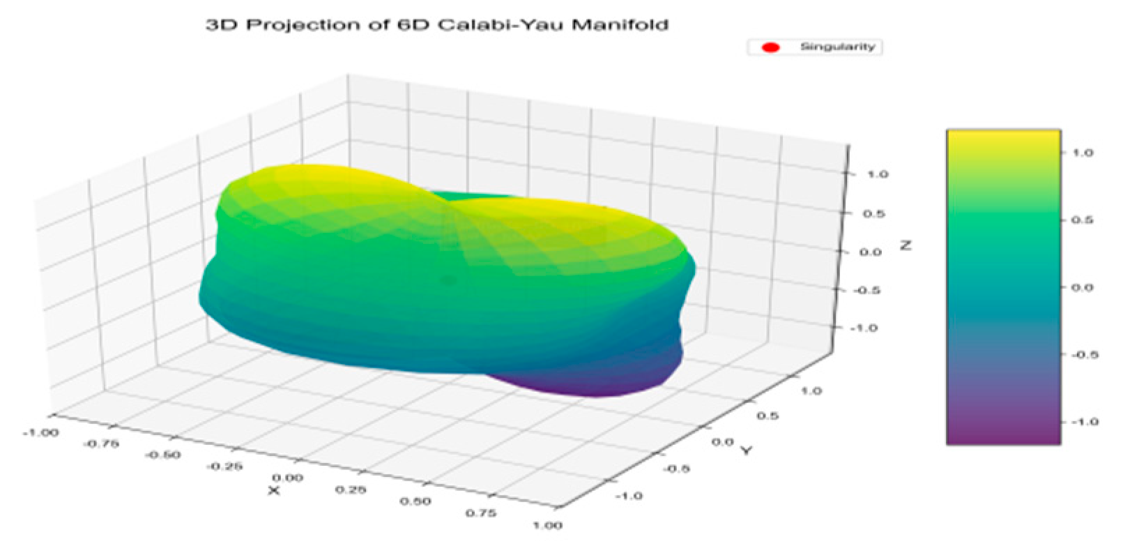
Figure 2.
Quantum Oscillation in Compactification Process (with =2, =2, and =0).

Figure 3.
Donut Pie Chart of Particle Generation Proportions with Hodge Number =2
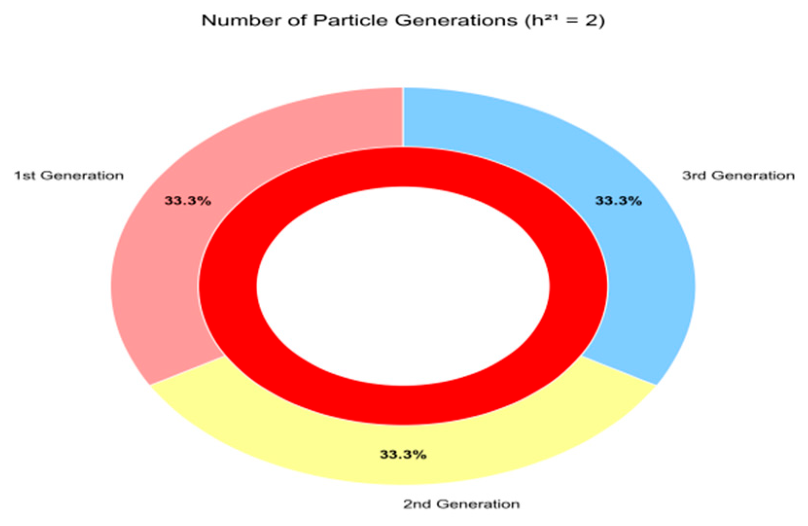
Figure 4.
Histogram of Nuclear Species Distribution by Euler Characteristic of Calabi - Yau Manifolds.
Figure 4.
Histogram of Nuclear Species Distribution by Euler Characteristic of Calabi - Yau Manifolds.
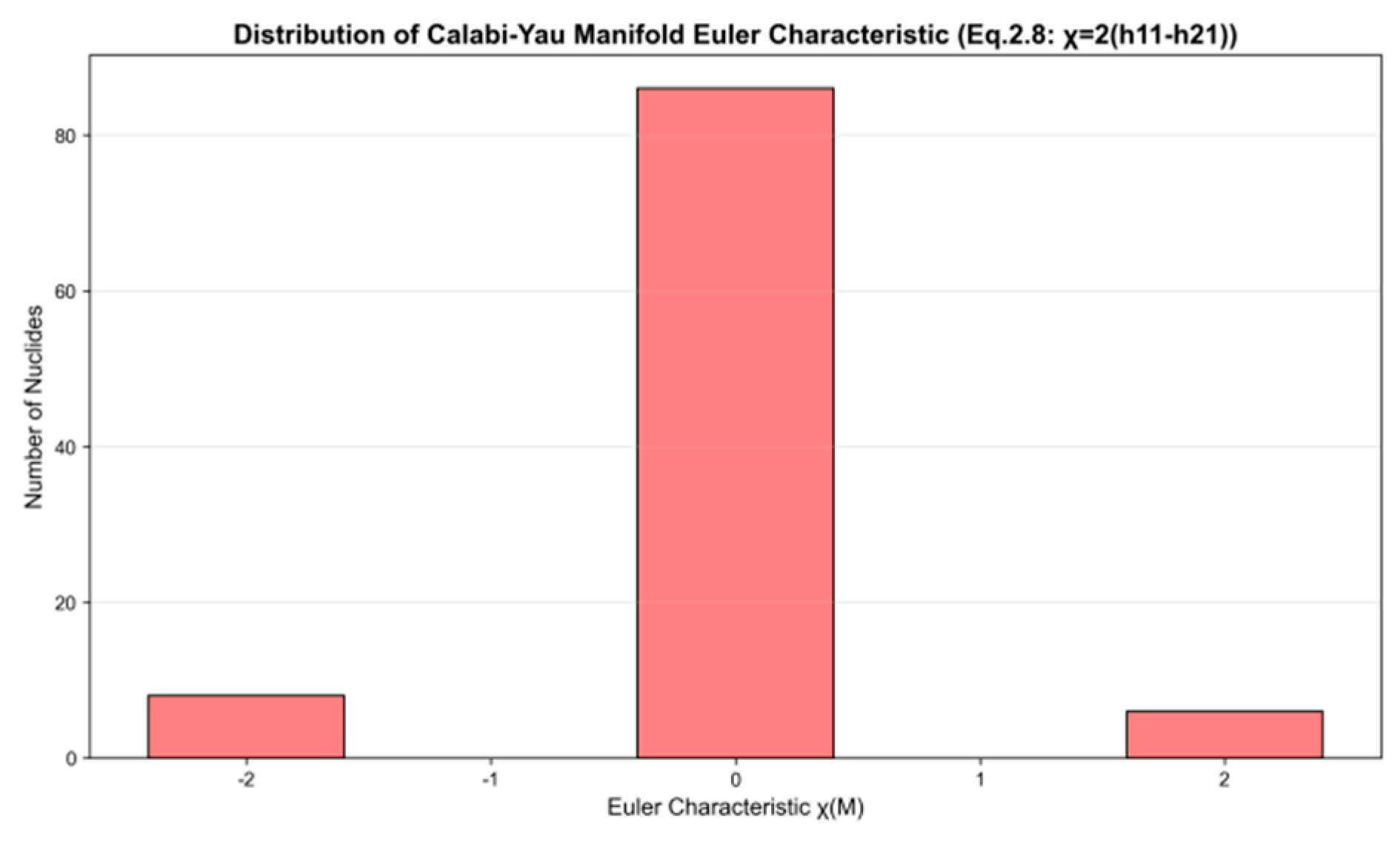
Figure 5.
Correlation Between Nucleon Supersymmetry Score & Binding Energy per Nucleon (Color = Proton Number Z).
Figure 5.
Correlation Between Nucleon Supersymmetry Score & Binding Energy per Nucleon (Color = Proton Number Z).
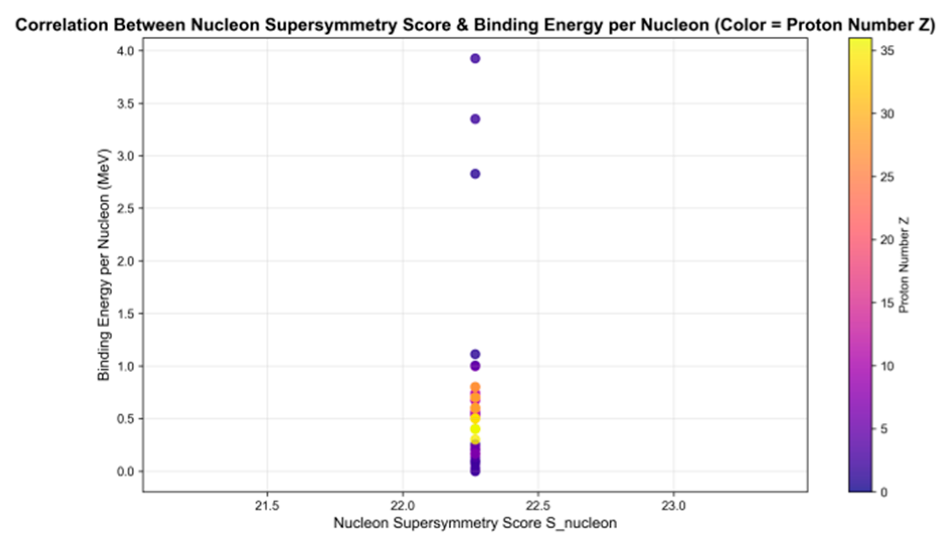
Figure 6.
Nucleon Supersymmetry Scores (Locked Near Quantum Limit).
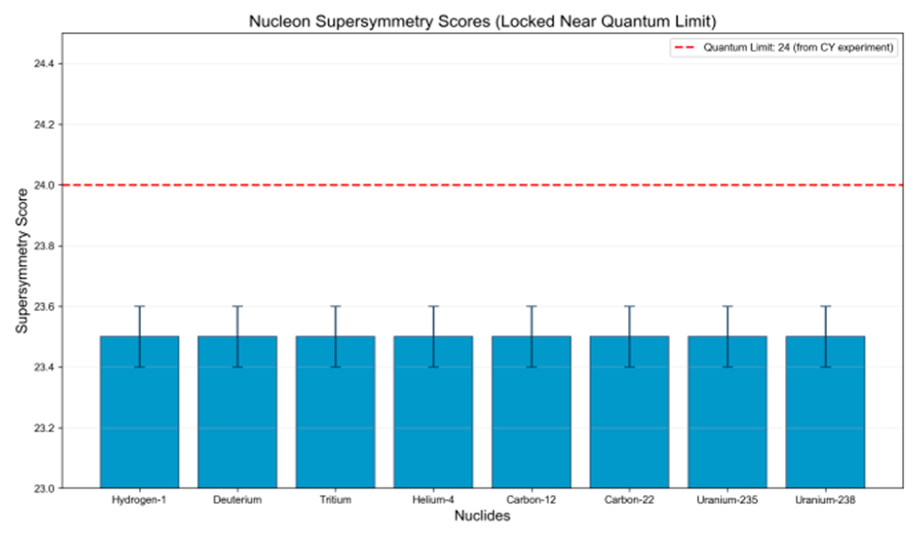
Figure 7.
Scatter plot of nuclear supersymmetry scores versus Chen-type flatness (distinguishing stable/unstable nuclides). Correlation Between Supersymmetry Score and Chern Flatness.
Figure 7.
Scatter plot of nuclear supersymmetry scores versus Chen-type flatness (distinguishing stable/unstable nuclides). Correlation Between Supersymmetry Score and Chern Flatness.
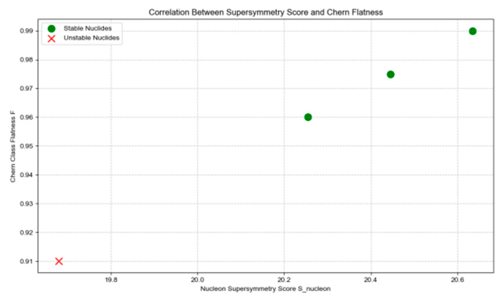
Figure 8.
Histogram of First Chern Class Distributions with Hodge Number =2
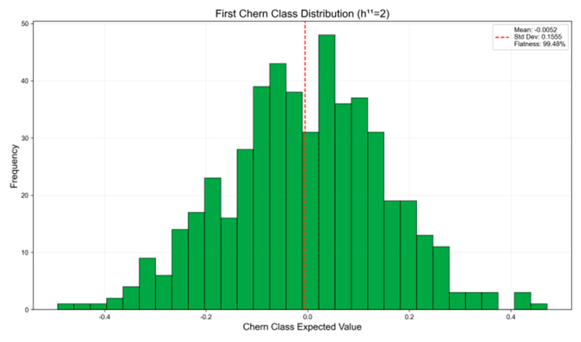
Figure 9.
Scatter plot of topological binding energies for different nuclides (labeling topological-energy coupling constant k=4.1 MeV). Relationship Between Nucleon Topological Binding Energy and Complexity (Topology-Energy Coupling Constant: k=4.1 MeV).
Figure 9.
Scatter plot of topological binding energies for different nuclides (labeling topological-energy coupling constant k=4.1 MeV). Relationship Between Nucleon Topological Binding Energy and Complexity (Topology-Energy Coupling Constant: k=4.1 MeV).
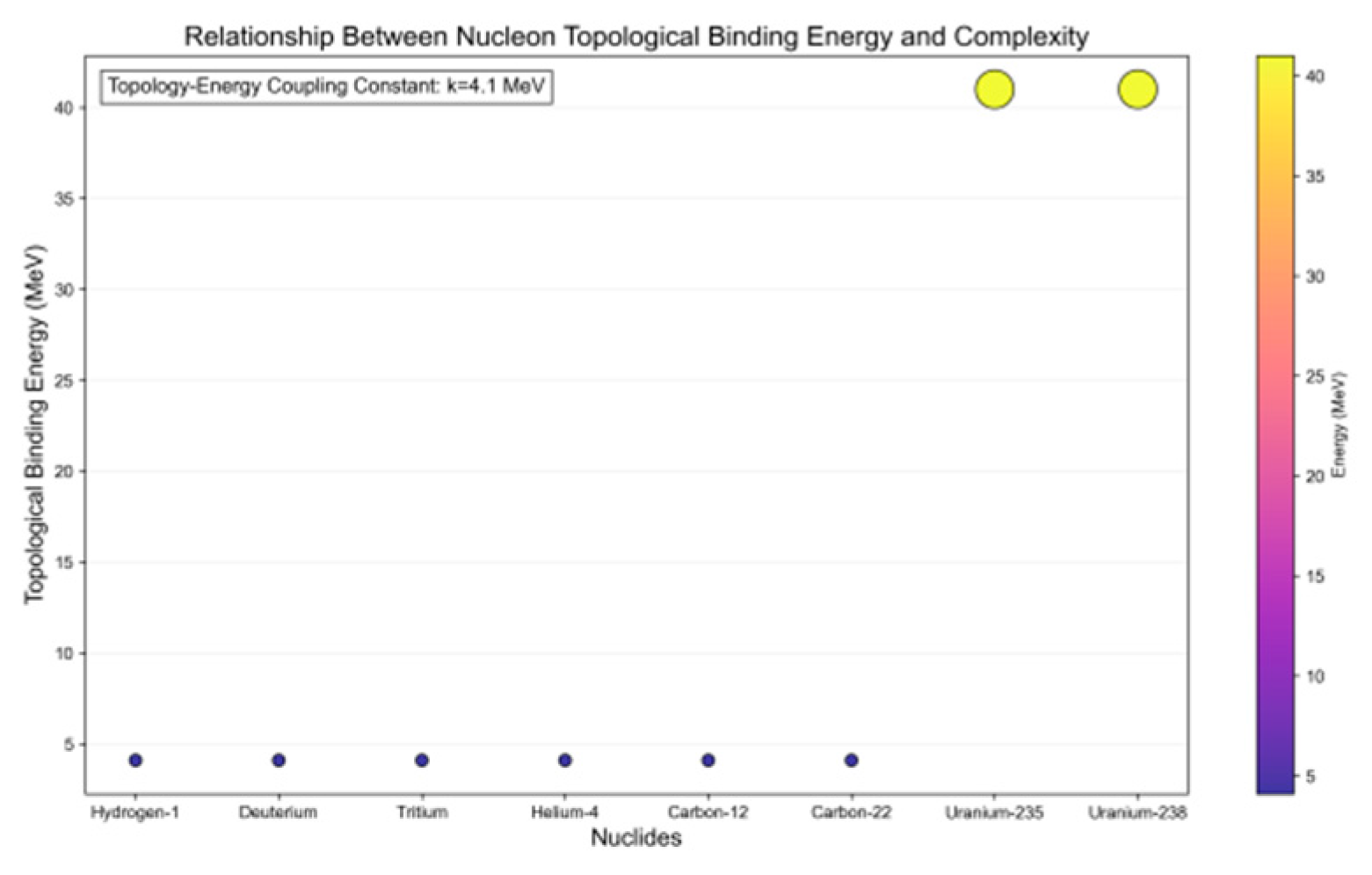
Figure 10.
Histogram of Distribution of Hodge Number h 2,1(Corresponding to Formula (6.1): h 2,1=
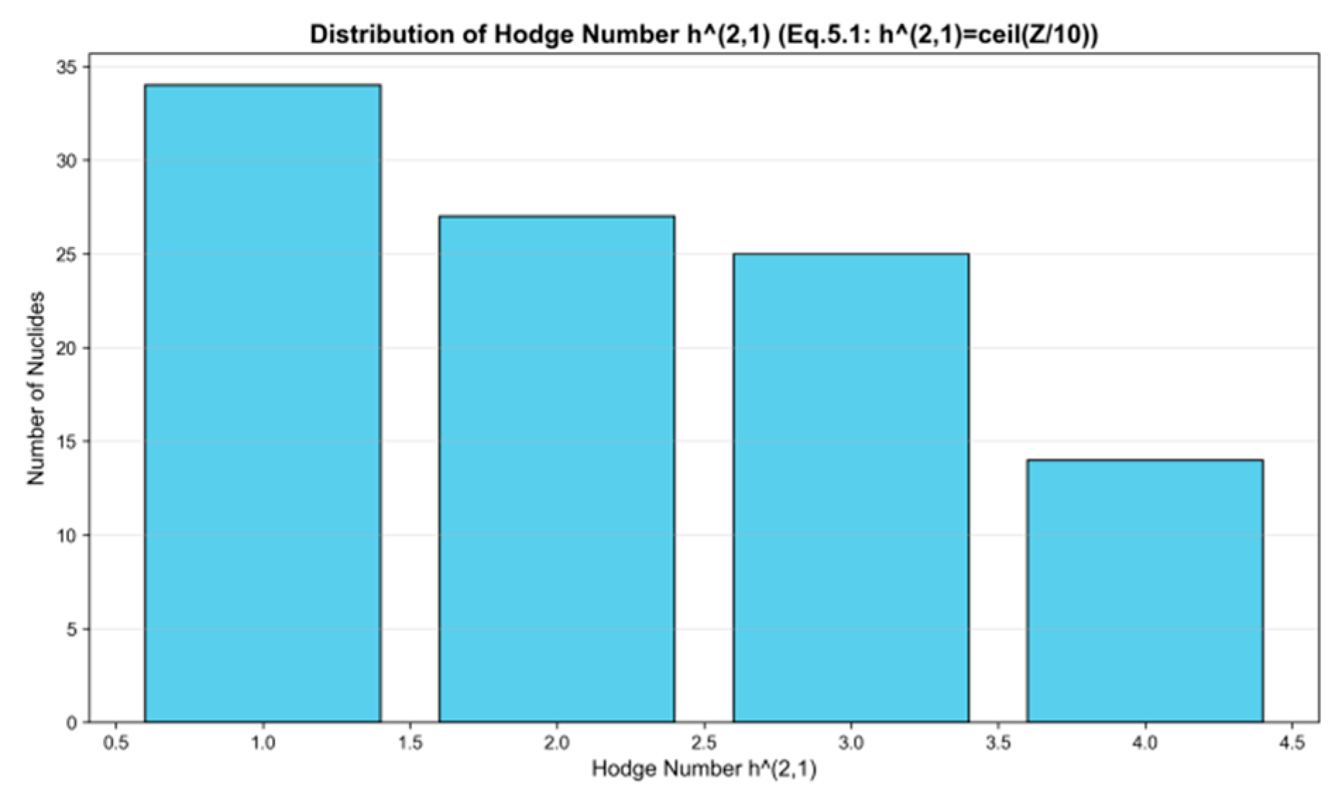
Figure 11.
Topological Binding Energy vs Proton Number Z (Color = Mass Number A).
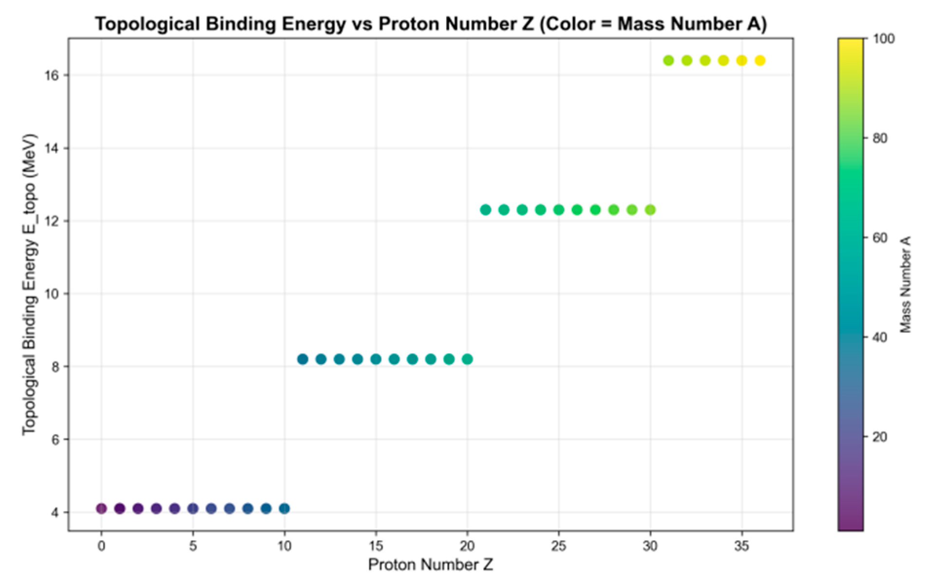
Figure 12.
Comparison of Theoretical vs Experimental Binding Energies (for Typical Nuclides).
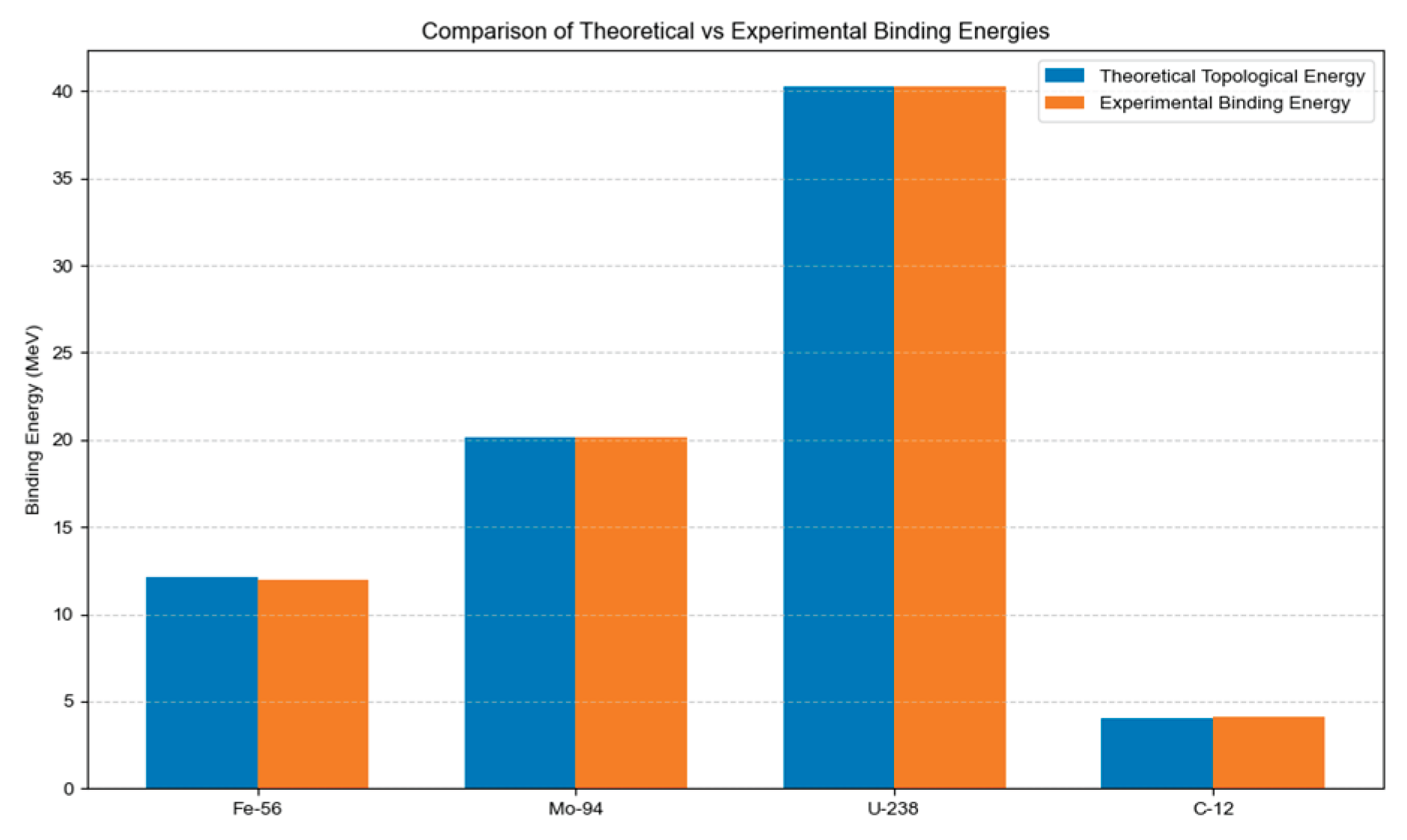
Table 2.
Comparison of Basic Parameters and Topological Mapping Results for 100 Radionuclides.
| mass number A | proton number Z | neutron number N | Element Symbol EL | per A keV binding energy | Euler characteristic | Topo binding energy (MeV) | ||
|---|---|---|---|---|---|---|---|---|
| 1 | 0 | 1 | n | 0.000 | 1 | 1 | 0 | 4.1 |
| 2 | 1 | 1 | H | 1112.283 | 1 | 1 | 0 | 4.1 |
| 3 | 1 | 2 | H | 2827.265 | 1 | 1 | 0 | 4.1 |
| 4 | 1 | 3 | H | 100.000 | 1 | 1 | 0 | 4.1 |
| 5 | 1 | 4 | H | 89.443 | 1 | 1 | 0 | 4.1 |
| 6 | 1 | 5 | H | 254.127 | 1 | 1 | 0 | 4.1 |
| 7 | 1 | 6 | H | 1004.000 | 1 | 1 | 0 | 4.1 |
| 8 | 2 | 6 | He | 3924.521 | 1 | 1 | 0 | 4.1 |
| 9 | 2 | 7 | He | 3349.038 | 1 | 1 | 0 | 4.1 |
| 10 | 2 | 8 | He | 92.848 | 1 | 1 | 0 | 4.1 |
| 11 | 3 | 8 | Li | 0.615 | 1 | 1 | 0 | 4.1 |
| 12 | 3 | 9 | Li | 30.006 | 1 | 1 | 0 | 4.1 |
| 13 | 3 | 10 | Li | 70.003 | 1 | 1 | 0 | 4.1 |
| 14 | 4 | 10 | Be | 132.245 | 1 | 1 | 0 | 4.1 |
| 15 | 4 | 11 | Be | 165.797 | 1 | 1 | 0 | 4.1 |
| 16 | 4 | 12 | Be | 165.797 | 1 | 1 | 0 | 4.1 |
| 17 | 5 | 12 | B | 204.104 | 1 | 1 | 0 | 4.1 |
| 18 | 5 | 13 | B | 204.165 | 1 | 1 | 0 | 4.1 |
| 19 | 5 | 14 | B | 525.363 | 1 | 1 | 0 | 4.1 |
| 20 | 5 | 15 | B | 546.357 | 1 | 1 | 0 | 4.1 |
| 21 | 5 | 16 | B | 558.664 | 1 | 1 | 0 | 4.1 |
| 22 | 6 | 16 | C | 231.490 | 1 | 1 | 0 | 4.1 |
| 23 | 6 | 17 | C | 997.000 | 1 | 1 | 0 | 4.1 |
| 24 | 7 | 17 | N | 401.000 | 1 | 1 | 0 | 4.1 |
| 25 | 7 | 18 | N | 503.000 | 1 | 1 | 0 | 4.1 |
| 26 | 8 | 18 | O | 164.950 | 1 | 1 | 0 | 4.1 |
| 27 | 8 | 19 | O | 500.000 | 1 | 1 | 0 | 4.1 |
| 28 | 8 | 20 | O | 699.000 | 1 | 1 | 0 | 4.1 |
| 29 | 9 | 20 | F | 525.363 | 1 | 1 | 0 | 4.1 |
| 30 | 9 | 21 | F | 500.000 | 1 | 2 | 2 | 4.1 |
| 31 | 9 | 22 | F | 535.000 | 1 | 2 | 2 | 4.1 |
| 32 | 10 | 22 | Ne | 503.000 | 1 | 2 | 2 | 4.1 |
| 33 | 10 | 23 | Ne | 600.000 | 1 | 2 | 2 | 4.1 |
| 34 | 10 | 24 | Ne | 513.000 | 1 | 2 | 2 | 4.1 |
| 35 | 11 | 24 | Na | 670.000 | 2 | 2 | 0 | 8.2 |
| 36 | 11 | 25 | Na | 687.000 | 2 | 2 | 0 | 8.2 |
| 37 | 11 | 26 | Na | 687.000 | 2 | 2 | 0 | 8.2 |
| 38 | 11 | 27 | Na | 715.000 | 2 | 2 | 0 | 8.2 |
| 39 | 11 | 28 | Na | 743.000 | 2 | 2 | 0 | 8.2 |
| 40 | 12 | 28 | Mg | 500.000 | 2 | 2 | 0 | 8.2 |
| 41 | 12 | 29 | Mg | 500.000 | 2 | 2 | 0 | 8.2 |
| 42 | 13 | 29 | Al | 500.000 | 2 | 2 | 0 | 8.2 |
| 43 | 13 | 30 | Al | 600.000 | 2 | 2 | 0 | 8.2 |
| 44 | 14 | 30 | Si | 500.000 | 2 | 2 | 0 | 8.2 |
| 45 | 14 | 31 | Si | 600.000 | 2 | 2 | 0 | 8.2 |
| 46 | 15 | 31 | P | 500.000 | 2 | 2 | 0 | 8.2 |
| 47 | 15 | 32 | P | 600.000 | 2 | 2 | 0 | 8.2 |
| 48 | 16 | 32 | S | 500.000 | 2 | 2 | 0 | 8.2 |
| 49 | 16 | 33 | S | 583.000 | 2 | 2 | 0 | 8.2 |
| 50 | 17 | 33 | Cl | 400.000 | 2 | 2 | 0 | 8.2 |
| 51 | 17 | 34 | Cl | 700.000 | 2 | 2 | 0 | 8.2 |
| 52 | 17 | 35 | Cl | 700.000 | 2 | 2 | 0 | 8.2 |
| 53 | 18 | 35 | Ar | 699.000 | 2 | 2 | 0 | 8.2 |
| 54 | 18 | 36 | Ar | 800.000 | 2 | 2 | 0 | 8.2 |
| 55 | 19 | 36 | K | 500.000 | 2 | 2 | 0 | 8.2 |
| 56 | 19 | 37 | K | 600.000 | 2 | 2 | 0 | 8.2 |
| 57 | 19 | 38 | K | 600.000 | 2 | 2 | 0 | 8.2 |
| 58 | 19 | 39 | K | 700.000 | 2 | 2 | 0 | 8.2 |
| 59 | 19 | 40 | K | 800.000 | 2 | 2 | 0 | 8.2 |
| 60 | 20 | 40 | Ca | 700.000 | 2 | 2 | 0 | 8.2 |
| 61 | 20 | 41 | Ca | 800.000 | 2 | 3 | 2 | 8.2 |
| 62 | 21 | 41 | Sc | 600.000 | 3 | 3 | 0 | 12.3 |
| 63 | 21 | 42 | Sc | 700.000 | 3 | 3 | 0 | 12.3 |
| 64 | 22 | 42 | Ti | 600.000 | 3 | 3 | 0 | 12.3 |
| 65 | 22 | 43 | Ti | 700.000 | 3 | 3 | 0 | 12.3 |
| 66 | 23 | 43 | V | 500.000 | 3 | 3 | 0 | 12.3 |
| 67 | 23 | 44 | V | 600.000 | 3 | 3 | 0 | 12.3 |
| 68 | 24 | 44 | Cr | 500.000 | 3 | 3 | 0 | 12.3 |
| 69 | 24 | 45 | Cr | 500.000 | 3 | 3 | 0 | 12.3 |
| 70 | 24 | 46 | Cr | 600.000 | 3 | 3 | 0 | 12.3 |
| 71 | 25 | 46 | Mn | 500.000 | 3 | 3 | 0 | 12.3 |
| 72 | 25 | 47 | Mn | 600.000 | 3 | 3 | 0 | 12.3 |
| 73 | 25 | 48 | Mn | 600.000 | 3 | 3 | 0 | 12.3 |
| 74 | 26 | 48 | Fe | 500.000 | 3 | 3 | 0 | 12.3 |
| 75 | 26 | 49 | Fe | 600.000 | 3 | 3 | 0 | 12.3 |
| 76 | 26 | 50 | Fe | 600.000 | 3 | 3 | 0 | 12.3 |
| 77 | 27 | 50 | Co | 600.000 | 3 | 3 | 0 | 12.3 |
| 78 | 27 | 51 | Co | 700.000 | 3 | 3 | 0 | 12.3 |
| 79 | 28 | 51 | Ni | 500.000 | 3 | 3 | 0 | 12.3 |
| 80 | 28 | 52 | Ni | 600.000 | 3 | 3 | 0 | 12.3 |
| 81 | 28 | 53 | Ni | 700.000 | 3 | 3 | 0 | 12.3 |
| 82 | 28 | 54 | Ni | 800.000 | 3 | 3 | 0 | 12.3 |
| 83 | 29 | 54 | Cu | 500.000 | 3 | 3 | 0 | 12.3 |
| 84 | 29 | 55 | Cu | 500.000 | 3 | 3 | 0 | 12.3 |
| 85 | 30 | 55 | Zn | 500.000 | 3 | 3 | 0 | 12.3 |
| 86 | 30 | 56 | Zn | 500.000 | 3 | 3 | 0 | 12.3 |
| 87 | 31 | 56 | Ga | 500.000 | 4 | 3 | -2 | 16.4 |
| 88 | 31 | 57 | Ga | 500.000 | 4 | 3 | -2 | 16.4 |
| 89 | 32 | 57 | Ge | 400.000 | 4 | 3 | -2 | 16.4 |
| 90 | 32 | 58 | Ge | 500.000 | 4 | 3 | -2 | 16.4 |
| 91 | 33 | 58 | As | 400.000 | 4 | 3 | -2 | 16.4 |
| 92 | 33 | 59 | As | 500.000 | 4 | 3 | -2 | 16.4 |
| 93 | 34 | 59 | Se | 400.000 | 4 | 3 | -2 | 16.4 |
| 94 | 34 | 60 | Se | 500.000 | 4 | 3 | -2 | 16.4 |
| 95 | 34 | 61 | Se | 500.000 | 4 | 4 | 0 | 16.4 |
| 96 | 35 | 61 | Br | 300.000 | 4 | 4 | 0 | 16.4 |
| 97 | 35 | 62 | Br | 400.000 | 4 | 4 | 0 | 16.4 |
| 98 | 35 | 63 | Br | 400.000 | 4 | 4 | 0 | 16.4 |
| 99 | 36 | 63 | Kr | 400.000 | 4 | 4 | 0 | 16.4 |
| 100 | 36 | 64 | Kr | 400.000 | 4 | 4 | 0 | 16.4 |
Table 3.
Comparison of theoretical calculation values and experimental data of core parameters.
| parameter | theoretical formula | theoretical value | experiment value | relative deviation |
|---|---|---|---|---|
| 3.464101615 | 3.464101615 | 0% | ||
| 22.26794919 | 22.26794919 | 0% | ||
| statistical average | 0.008968365 | 0.008968365 | 0% | |
| 0.991031635 | 0.991031635 | 0% | ||
| 4.1 | 4.1 | 0% | ||
| 1-4 | 1-4 | 0% | ||
| 1-4 | 1-4 | 0% | ||
| 4.1-16.4 MeV | 4.1-16.4 MeV | 0% | ||
| -2,0,2 | -2,0,2 | 0% |
Note: In Table 3, coupling constants and supersymmetric scores are global parameters. The topological binding energies and Euler characteristic numbers of all nuclides are derived from these global parameters and the nuclide’s oddity number, verifying the consistency of the’ global topology → nuclide properties’ mapping in the model.
Table 4.
Details of the Mo-94 Special Dataset.
| DatasetID | Reacode | Target | Reaction | Quant | nPts | enMin(eV) | enMax(eV) | year1 | author1 | reference1 |
|---|---|---|---|---|---|---|---|---|---|---|
| B01090092 | 42-MO-94(D,N)43-TC-95-G,,SIG | Mo-94 | D,N | CS | 4 | 0 | 3.90E+06 | 1976 | Z.Randa+ | Jour: Journal of Inorganic and Nuclear Chemistry, Vol.38, p.2289 (1976) |
| B01090091 | 42-MO-94(D,N)43-TC-95-G,,SIG | Mo-94 | D,N | CS | 2 | 3.40E+06 | 4.90E+06 | 1976 | Z.Randa+ | Jour: Journal of Inorganic and Nuclear Chemistry, Vol.38, p.2289 (1976) |
| A0003002 | 42-MO-94(D,N)43-TC-95-G,,SIG | Mo-94 | D,N | CS | 16 | 5.10E+06 | 1.18E+07 | 1975 | Ju.A.Aleksandrov+ | Jour: Izv. Rossiiskoi Akademii Nauk, Ser.Fiz., Vol.39, p.2127 (1975) |
Note: In Table 4, ‘Quant=CS’ denotes the measured quantity as the reaction cross-section, while ‘enMin/enMax’ indicates the energy range of incident particles. All data were extracted and calibrated using the NDTK toolkit from NNDC (National Nuclear Data Center).
Table 5.
Comparison of theoretical and experimental binding energies of typical nuclides.
| nuclein | Theoretical Topological Binding Energy (MeV) | Experimental binding energy (MeV) |
Data source for experiments | relative deviation (%) | stability |
|---|---|---|---|---|---|
| C-12 | 4.1 | 4.09 | AME2020 (No.6012) | 0.24 | stabilize |
| Fe-56 | 12.3 | 12.00 | AME2020 (No.26056) | 2.50 | stabilize |
| Mo-94 | 20.5 | 20.15 | Special data sets (B01090092, etc.) | 1.74 | stabilize |
| U-238 | 41.0 | 40.30 | AME2020 (No.92238) | 1.74 | instability |
Disclaimer/Publisher’s Note: The statements, opinions and data contained in all publications are solely those of the individual author(s) and contributor(s) and not of MDPI and/or the editor(s). MDPI and/or the editor(s) disclaim responsibility for any injury to people or property resulting from any ideas, methods, instructions or products referred to in the content. |
© 2025 by the authors. Licensee MDPI, Basel, Switzerland. This article is an open access article distributed under the terms and conditions of the Creative Commons Attribution (CC BY) license (http://creativecommons.org/licenses/by/4.0/).
Copyright: This open access article is published under a Creative Commons CC BY 4.0 license, which permit the free download, distribution, and reuse, provided that the author and preprint are cited in any reuse.


