
Submitted:
10 September 2025
Posted:
10 September 2025
You are already at the latest version
Abstract
Precise determination of nuclear radii and charge radii is a cornerstone of nuclear physics, essential for understanding nuclear structure, reaction dynamics, and astrophysical phenomena. Traditional empirical models often include numerous corrections to address isotopic asymmetry, shell effects, and pairing energies, resulting in complex formulae with many fitted parameters that restrict practical use. Building on the 4G model of final unification, this work introduces a simplified, physically motivated nuclear radius framework. It separately accounts for proton and neutron contributions based on their cubic root form and incorporates an adjustable mass distribution coefficient (Cmd), empirically dependent on the fine structure ratio and the strong coupling constant. Crucially, the mass radius is formulated as the product of (Cmd) and the nuclear charge radius—a feature that directly relates unified scaling parameters to experimentally accessible quantities. Close to the stable mass numbers of Z = (2 to 118), Cmd = (1.127 to 1.382). It needs fine tuning. This novel approach’s predictive performance is rigorously benchmarked against advanced formulae incorporating detailed nuclear structure corrections. Results show that this minimalistic method achieves accuracy comparable to complex models across a broad range of nuclei while substantially reducing computational complexity. It thus provides an efficient and physically transparent tool for rapid nuclear radius estimation, suitable for both theoretical studies and practical nuclear science applications.
Keywords:
nuclear mass radius
; nuclear charge radius
; mass distribution coefficient
; proton and neutron contributions
; fine structure ratio
; strong coupling constant
; 4G model of final unification
1. Introduction
The nuclear radius is a primary characteristic of atomic nuclei, influencing cross sections, decay properties, and nuclear matter distributions. Traditionally, the nuclear radius RA is approximated by the empirical formula [1]:
where A=Z+N is the mass number, and R0 is a constant of about 1.2–1.3 fm. However, as experimental data and theoretical understanding advanced, formulas began incorporating corrections for proton-neutron asymmetry, pairing, shell closures, and surface diffuseness to improve accuracy, leading to complex multi-term models [2,3,4,5,6,7,8].
Despite these improvements, the complexity restricts practical use, especially in applications requiring quick estimates or large-scale computations. Motivated by this, we investigate a simple formula for mass distribution radius [9,10,11]:
where Rp is a 4G model of characteristic radius constant associated with proton and Cmd is a coefficient that can be empirically tuned. This respects the separate roles of protons and neutrons in nuclear size and offers flexibility with a minimal parameter set.
2. Three Assumptions and Two Applications of Our 4G Model of Final Unification
- (1)
- There exists a characteristic electroweak fermion of rest energy, . It can be considered as the zygote of all elementary particles.
- (2)
- There exists a nuclear elementary charge in such a way that, = Strong coupling constant and .
- (3)
- Each atomic interaction is associated with a characteristic large gravitational coupling constant. Their fitted magnitudes are,
It may be noted that,
- (1)
- In a unified approach, most important point to be noted is that,
Clearly speaking, based on the electroweak interaction, the well believed quantum constant seems to have a deep inner meaning. Following this kind of relation, there is a possibility to understand the integral nature of quantum mechanics with a relation of the form, It needs further study with reference to EPR argument [12].
- (2)
- Another interesting application is that, string theory [9] can be made practical with reference to the three atomic gravitational constants associated with weak, strong, and electromagnetic interaction gravitational constants. These constants provide a framework to bridge the gap between quantum mechanics and gravity at the atomic scale, offering new insights into particle interactions. By incorporating these gravitational couplings into string theory models, it becomes possible to explore unified descriptions of fundamental forces. This approach may lead to testable predictions linking microscopic string dynamics with observable nuclear phenomena, thereby advancing both theoretical and experimental physics. See Table 1. and Table 2. for sample string tensions and energies without any coupling constants.
- (3)
- Weak interaction point of view [13], following our assumptions, Fermi’s weak coupling constant can be fitted with the following relations.
3. Formula Development and Methodology
3.1. Advanced Nuclear Mass Radius Formula
We adopt an advanced mass radius formula [14,15,16,17,18,19,20] used in nuclear physics literature incorporating empirical corrections for nuclear structure effects:
where
- ➢
- The aA1/3 base term originates from the classic geometric model of the nucleus, where the radius scales with the cube root of the mass number, describing the approximate constancy of nuclear density across the chart.
- ➢
- The bI isospin asymmetry term I=(N−Z)/A represents the correction for neutron-proton imbalance, which is known to influence nuclear size and is included in several radius fitting studies.
- ➢
- The cδ pairing correction accounts for the variation in nuclear radii depending on whether the nucleus has even or odd numbers of protons and neutrons; such terms appear in both mass and radius systematics.
- ➢
- The dA−1/3 inverse scaling term and the constant e are added for additional fitting flexibility and improved regression accuracy.
- ➢
- The fS shell correction term incorporates effects from nuclear shell structure, particularly close to magic numbers, as described in various empirical and theoretical studies
- ➢
- a,b,c,d,e,f are coefficients fitted to experimental data.
- ➢
- This formula is given by AI by considering so many references. It needs proper citation and confirmation. For the time being, we consider it as an advanced mass radius formula. For details, see the python program presented in section (6).
- ➢
- It is very interesting to note that, numerically, output of this advanced mass radius relation can be compared with 4G model relation, See Table 3, columns 4 and 5.
- ➢
- This formula captures detailed nuclear structure features but involves multiple fitted parameters and terms.
3.2. Proposed Simple Formula
It may be noted that, the mass radius and charge radius of atomic nuclides are related but distinct nuclear properties, each reflecting different aspects of nuclear structure:
- (A)
- Mass Radius:
- (1)
- The mass radius refers to the spatial extent of the total nuclear mass distribution, considering both protons and neutrons as massive particles within the nucleus.
- (2)
- It describes the radius at which the nuclear matter density drops to half its central value and is defined through gravitational form factors or nuclear density profiles.
- (3)
- Mass radii can be probed in specialized reactions and models but are not directly measured in typical scattering experiments.
- (B)
- Charge Radius:
- (1)
- The charge radius is the root-mean-square (rms) distance of the distribution of the proton (electric charge) density inside the nucleus.
- (2)
- It is measured directly by high-precision experiments, such as elastic electron scattering, muonic atom spectroscopy, or optical isotope shifts, since these techniques respond to the nuclear electric field produced by protons.
- (3)
- The charge radius is particularly sensitive to the spatial arrangement of protons, not neutrons, in the nucleus.
- (C)
- Key Differences:
- (1)
- The mass radius reflects the distribution of all nucleons (protons and neutrons), while the charge radius primarily describes the distribution of protons only.
- (2)
- Experimental nuclear charge radii are typically slightly smaller than mass radii in nuclei with a neutron excess, because neutron-rich nuclei have a more extended neutron distribution (sometimes called a neutron skin).
- (3)
- In some light nuclei (e.g., 4He), mass radius and charge radius can be nearly identical due to similar proton and neutron distributions, but differences become apparent in heavier or neutron-rich nuclei.
- (D)
- Proposed Formulae
Close to the stable mass numbers of any Z, we propose the mass radius Rmd as follows.
For Z > 1,
[21]
For estimating the mass radii of isotopes of Z=2 to 118, we are working on refining this mass distribution coefficient with reference to fine structure constant [21], strong coupling constant [22,23] and the approximate stable mass numbers of Z [9,10,11]. With further study, things can be improved well and back ground physics can be explored in a unified approach. One such approximate relation can be expressed as,
Based on relations (6) and (7), it is possible to give some physical meaning to the proposed mass distribution factor as follows. With reference to nuclear charge radius,
- (1)
- Fine structure ratio helps in increasing the mass distribution radius by a factor of
- (2)
- Strong coupling coefficient helps in increasing the mass distribution by a factor of.
- (3)
- Close to stable mass numbers, mass distribution radius takes the following form,
- (4)
- Above and below the stable mass numbers, mass distribution radius takes the following form,
4. Results: Figures and Data Table
The key phenomenological scaling factor “0.0016 appearing in our proposed nuclear line of beta stability is the ratio of the geometric mean of the charged and neutral pion masses (~137.26 MeV) to that of the weak boson masses (~85.61 GeV), which numerically evaluates to approximately 0.0016. This dimensionless ratio encapsulates the profound hierarchical gap between the strong interaction scale and the electroweak scale and forms a cornerstone of the mass relations underlying our 585 GeV electroweak fermion. Importantly, this ratio is not merely a numerical coincidence but has substantive implications for understanding nuclear stability and nuclear binding energy. The interplay of these fundamental mass scales suggests that the dynamics governing nuclear forces and nucleon interactions may be intimately connected to electroweak-scale physics mediated by the 585 GeV fermion. For a deeper exploration of how this mass ratio informs nuclear binding mechanisms and stability criteria, interested readers are encouraged to refer our recent preprints and other peer-reviewed publications [24,25], where these connections are discussed in detail with complementary theoretical and phenomenological analyses.
Based on this electroweak coefficient , stability corresponding to nuclear beta decay can be understood with the following relation.
One can find a similar relation in the literature. This relation can be well tested for Z=21 to 92. For example,
This is one best practical and quantitative application of our proposed electroweak fermion and bosons. Following this relation and based on various semi empirical mass formulae [26,27], by knowing any stable mass number, its corresponding proton number can be estimated with,
Based on these relations and concepts, we have prepared Table 3 & Figure 1 for the approximate stable mass numbers of Z=2 to 118. See Figure 2, Figure 3, Figure 4, Figure 5, Figure 6, Figure 7, Figure 8 for the isotopes of the magic numbers 2,8,20,28,50,82 and 114.
The simple formula with minimal fitting achieves less than 2% error for medium to heavy nuclei and reasonable accuracy even for lighter nuclei, apart from extremely light cases like He-4 where nuclear structure effects dominate beyond mass scaling.

Table 3.
Approximate fitting of nuclear mass radii based on cubic root of proton and neutron numbers.
Table 3.
Approximate fitting of nuclear mass radii based on cubic root of proton and neutron numbers.
| Z | N | Approximate stable mass number (As) |
Advanced Mass Radius (fm) | A(1/3)*1.24 (fm) |
Estimated Nuclear Charge Radius [28] (fm) | Mass Distribution Factor | Estimated Mass Radius (fm) |
Error (fm) |
Percentage Error (%) |
|---|---|---|---|---|---|---|---|---|---|
| 2 | 2 | 4 | 1.695 | 1.968 | 1.562 | 1.127 | 1.760 | -0.065 | 3.84 |
| 3 | 3 | 6 | 2.071 | 2.253 | 1.788 | 1.177 | 2.106 | -0.035 | 1.67 |
| 4 | 4 | 8 | 2.315 | 2.480 | 1.968 | 1.191 | 2.345 | -0.03 | 1.28 |
| 5 | 5 | 10 | 2.562 | 2.671 | 2.120 | 1.200 | 2.544 | 0.018 | 0.70 |
| 6 | 6 | 12 | 2.712 | 2.839 | 2.253 | 1.206 | 2.717 | -0.005 | 0.17 |
| 7 | 7 | 14 | 2.906 | 2.989 | 2.372 | 1.211 | 2.872 | 0.034 | 1.16 |
| 8 | 8 | 16 | 3.032 | 3.125 | 2.480 | 1.215 | 3.013 | 0.019 | 0.63 |
| 9 | 10 | 19 | 3.293 | 3.309 | 2.594 | 1.222 | 3.169 | 0.124 | 3.75 |
| 10 | 11 | 21 | 3.317 | 3.421 | 2.686 | 1.224 | 3.289 | 0.028 | 0.84 |
| 11 | 12 | 23 | 3.517 | 3.526 | 2.771 | 1.227 | 3.401 | 0.116 | 3.30 |
| 12 | 13 | 25 | 3.525 | 3.626 | 2.852 | 1.230 | 3.507 | 0.018 | 0.52 |
| 13 | 14 | 27 | 3.743 | 3.720 | 2.928 | 1.232 | 3.608 | 0.135 | 3.60 |
| 14 | 15 | 29 | 3.740 | 3.810 | 3.000 | 1.235 | 3.704 | 0.036 | 0.95 |
| 15 | 16 | 31 | 3.917 | 3.895 | 3.069 | 1.237 | 3.797 | 0.12 | 3.08 |
| 16 | 18 | 34 | 3.994 | 4.017 | 3.145 | 1.241 | 3.902 | 0.092 | 2.30 |
| 17 | 19 | 36 | 4.102 | 4.094 | 3.208 | 1.243 | 3.987 | 0.115 | 2.81 |
| 18 | 20 | 38 | 4.157 | 4.169 | 3.269 | 1.245 | 4.068 | 0.089 | 2.12 |
| 19 | 21 | 40 | 4.259 | 4.241 | 3.327 | 1.247 | 4.148 | 0.111 | 2.60 |
| 20 | 23 | 43 | 4.290 | 4.344 | 3.392 | 1.249 | 4.239 | 0.051 | 1.21 |
| 21 | 24 | 45 | 4.461 | 4.411 | 3.447 | 1.251 | 4.313 | 0.148 | 3.33 |
| 22 | 25 | 47 | 4.430 | 4.475 | 3.499 | 1.253 | 4.385 | 0.045 | 1.01 |
| 23 | 26 | 49 | 4.611 | 4.538 | 3.551 | 1.255 | 4.455 | 0.156 | 3.38 |
| 24 | 28 | 52 | 4.655 | 4.628 | 3.608 | 1.257 | 4.536 | 0.119 | 2.55 |
| 25 | 29 | 54 | 4.727 | 4.687 | 3.656 | 1.259 | 4.603 | 0.124 | 2.62 |
| 26 | 30 | 56 | 4.763 | 4.744 | 3.703 | 1.261 | 4.668 | 0.095 | 1.98 |
| 27 | 32 | 59 | 4.898 | 4.827 | 3.755 | 1.263 | 4.743 | 0.155 | 3.16 |
| 28 | 33 | 61 | 4.855 | 4.881 | 3.800 | 1.265 | 4.806 | 0.049 | 1.02 |
| 29 | 34 | 63 | 5.011 | 4.934 | 3.844 | 1.266 | 4.867 | 0.144 | 2.87 |
| 30 | 36 | 66 | 5.040 | 5.011 | 3.892 | 1.268 | 4.937 | 0.103 | 2.04 |
| 31 | 37 | 68 | 5.118 | 5.061 | 3.934 | 1.270 | 4.996 | 0.122 | 2.39 |
| 32 | 39 | 71 | 5.118 | 5.135 | 3.980 | 1.272 | 5.063 | 0.055 | 1.08 |
| 33 | 40 | 73 | 5.268 | 5.182 | 4.020 | 1.273 | 5.120 | 0.148 | 2.83 |
| 34 | 41 | 75 | 5.218 | 5.229 | 4.059 | 1.275 | 5.175 | 0.043 | 0.82 |
| 35 | 43 | 78 | 5.363 | 5.298 | 4.103 | 1.277 | 5.239 | 0.124 | 2.32 |
| 36 | 44 | 80 | 5.400 | 5.343 | 4.141 | 1.278 | 5.293 | 0.107 | 1.99 |
| 37 | 46 | 83 | 5.518 | 5.409 | 4.183 | 1.280 | 5.354 | 0.164 | 2.97 |
| 38 | 47 | 85 | 5.448 | 5.452 | 4.219 | 1.282 | 5.406 | 0.042 | 0.77 |
| 39 | 49 | 88 | 5.588 | 5.515 | 4.259 | 1.283 | 5.466 | 0.122 | 2.19 |
| 40 | 50 | 90 | 5.607 | 5.557 | 4.294 | 1.285 | 5.517 | 0.09 | 1.61 |
| 41 | 52 | 93 | 5.719 | 5.618 | 4.333 | 1.286 | 5.574 | 0.145 | 2.53 |
| 42 | 53 | 95 | 5.661 | 5.658 | 4.367 | 1.288 | 5.623 | 0.038 | 0.66 |
| 43 | 55 | 98 | 5.796 | 5.717 | 4.404 | 1.290 | 5.680 | 0.116 | 2.01 |
| 44 | 56 | 100 | 5.812 | 5.756 | 4.437 | 1.291 | 5.728 | 0.084 | 1.45 |
| 45 | 58 | 103 | 5.920 | 5.813 | 4.474 | 1.292 | 5.782 | 0.138 | 2.33 |
| 46 | 60 | 106 | 5.927 | 5.868 | 4.510 | 1.294 | 5.836 | 0.091 | 1.53 |
| 47 | 61 | 108 | 5.990 | 5.905 | 4.541 | 1.295 | 5.882 | 0.108 | 1.81 |
| 48 | 63 | 111 | 5.971 | 5.959 | 4.576 | 1.297 | 5.935 | 0.036 | 0.60 |
| 49 | 64 | 113 | 6.108 | 5.995 | 4.606 | 1.298 | 5.980 | 0.128 | 2.10 |
| 50 | 66 | 116 | 6.112 | 6.047 | 4.640 | 1.300 | 6.031 | 0.081 | 1.32 |
| 51 | 68 | 119 | 6.214 | 6.099 | 4.673 | 1.301 | 6.082 | 0.132 | 2.14 |
| 52 | 69 | 121 | 6.150 | 6.133 | 4.702 | 1.303 | 6.125 | 0.025 | 0.40 |
| 53 | 71 | 124 | 6.291 | 6.183 | 4.735 | 1.304 | 6.175 | 0.116 | 1.85 |
| 54 | 73 | 127 | 6.267 | 6.233 | 4.767 | 1.306 | 6.224 | 0.043 | 0.69 |
| 55 | 74 | 129 | 6.386 | 6.265 | 4.795 | 1.307 | 6.266 | 0.12 | 1.87 |
| 56 | 76 | 132 | 6.385 | 6.314 | 4.826 | 1.308 | 6.314 | 0.071 | 1.11 |
| 57 | 78 | 135 | 6.483 | 6.361 | 4.857 | 1.310 | 6.361 | 0.122 | 1.88 |
| 58 | 80 | 138 | 6.481 | 6.408 | 4.887 | 1.311 | 6.408 | 0.073 | 1.12 |
| 59 | 81 | 140 | 6.538 | 6.439 | 4.914 | 1.312 | 6.449 | 0.089 | 1.36 |
| 60 | 83 | 143 | 6.510 | 6.484 | 4.944 | 1.314 | 6.495 | 0.015 | 0.23 |
| 61 | 85 | 146 | 6.631 | 6.529 | 4.973 | 1.315 | 6.540 | 0.091 | 1.36 |
| 62 | 87 | 149 | 6.601 | 6.574 | 5.002 | 1.317 | 6.585 | 0.016 | 0.23 |
| 63 | 88 | 151 | 6.731 | 6.603 | 5.027 | 1.318 | 6.625 | 0.106 | 1.58 |
| 64 | 90 | 154 | 6.726 | 6.647 | 5.056 | 1.319 | 6.669 | 0.057 | 0.84 |
| 65 | 92 | 157 | 6.819 | 6.689 | 5.084 | 1.320 | 6.713 | 0.106 | 1.56 |
| 66 | 94 | 160 | 6.812 | 6.732 | 5.112 | 1.322 | 6.756 | 0.056 | 0.82 |
| 67 | 96 | 163 | 6.905 | 6.774 | 5.139 | 1.323 | 6.799 | 0.106 | 1.53 |
| 68 | 98 | 166 | 6.897 | 6.815 | 5.166 | 1.324 | 6.842 | 0.055 | 0.80 |
| 69 | 99 | 168 | 6.951 | 6.842 | 5.190 | 1.326 | 6.880 | 0.071 | 1.02 |
| 70 | 101 | 171 | 6.917 | 6.883 | 5.217 | 1.327 | 6.922 | -0.005 | 0.07 |
| 71 | 103 | 174 | 7.033 | 6.923 | 5.243 | 1.328 | 6.963 | 0.07 | 0.98 |
| 72 | 105 | 177 | 6.998 | 6.962 | 5.269 | 1.329 | 7.005 | -0.007 | 0.10 |
| 73 | 107 | 180 | 7.113 | 7.001 | 5.295 | 1.331 | 7.046 | 0.067 | 0.94 |
| 74 | 109 | 183 | 7.077 | 7.040 | 5.320 | 1.332 | 7.087 | -0.01 | 0.13 |
| 75 | 111 | 186 | 7.191 | 7.078 | 5.346 | 1.333 | 7.127 | 0.064 | 0.89 |
| 76 | 113 | 189 | 7.155 | 7.116 | 5.371 | 1.334 | 7.167 | -0.012 | 0.17 |
| 77 | 115 | 192 | 7.268 | 7.154 | 5.396 | 1.336 | 7.207 | 0.061 | 0.84 |
| 78 | 117 | 195 | 7.231 | 7.191 | 5.420 | 1.337 | 7.246 | -0.015 | 0.22 |
| 79 | 119 | 198 | 7.343 | 7.227 | 5.445 | 1.338 | 7.286 | 0.057 | 0.78 |
| 80 | 121 | 201 | 7.305 | 7.264 | 5.469 | 1.339 | 7.325 | -0.02 | 0.27 |
| 81 | 123 | 204 | 7.417 | 7.300 | 5.493 | 1.341 | 7.363 | 0.054 | 0.72 |
| 82 | 125 | 207 | 7.378 | 7.335 | 5.516 | 1.342 | 7.402 | -0.024 | 0.32 |
| 83 | 127 | 210 | 7.489 | 7.370 | 5.540 | 1.343 | 7.440 | 0.049 | 0.65 |
| 84 | 129 | 213 | 7.450 | 7.405 | 5.563 | 1.344 | 7.478 | -0.028 | 0.38 |
| 85 | 131 | 216 | 7.560 | 7.440 | 5.586 | 1.345 | 7.516 | 0.044 | 0.58 |
| 86 | 133 | 219 | 7.520 | 7.474 | 5.609 | 1.347 | 7.553 | -0.033 | 0.44 |
| 87 | 135 | 222 | 7.629 | 7.508 | 5.632 | 1.348 | 7.590 | 0.039 | 0.51 |
| 88 | 138 | 226 | 7.650 | 7.553 | 5.657 | 1.349 | 7.631 | 0.019 | 0.24 |
| 89 | 140 | 229 | 7.733 | 7.586 | 5.679 | 1.350 | 7.668 | 0.065 | 0.85 |
| 90 | 142 | 232 | 7.717 | 7.619 | 5.701 | 1.351 | 7.704 | 0.013 | 0.17 |
| 91 | 144 | 235 | 7.800 | 7.652 | 5.723 | 1.352 | 7.740 | 0.06 | 0.77 |
| 92 | 146 | 238 | 7.783 | 7.684 | 5.745 | 1.354 | 7.777 | 0.006 | 0.09 |
| 93 | 148 | 241 | 7.866 | 7.717 | 5.767 | 1.355 | 7.812 | 0.054 | 0.68 |
| 94 | 151 | 245 | 7.809 | 7.759 | 5.791 | 1.356 | 7.852 | -0.043 | 0.55 |
| 95 | 153 | 248 | 7.916 | 7.791 | 5.812 | 1.357 | 7.887 | 0.029 | 0.36 |
| 96 | 155 | 251 | 7.873 | 7.822 | 5.833 | 1.358 | 7.922 | -0.049 | 0.63 |
| 97 | 157 | 254 | 7.980 | 7.853 | 5.854 | 1.359 | 7.957 | 0.023 | 0.28 |
| 98 | 159 | 257 | 7.936 | 7.884 | 5.875 | 1.360 | 7.992 | -0.056 | 0.71 |
| 99 | 162 | 261 | 8.077 | 7.924 | 5.898 | 1.362 | 8.030 | 0.047 | 0.58 |
| 100 | 164 | 264 | 8.058 | 7.955 | 5.918 | 1.363 | 8.065 | -0.007 | 0.09 |
| 101 | 166 | 267 | 8.138 | 7.985 | 5.939 | 1.364 | 8.099 | 0.039 | 0.48 |
| 102 | 169 | 271 | 8.078 | 8.024 | 5.961 | 1.365 | 8.137 | -0.059 | 0.72 |
| 103 | 171 | 274 | 8.183 | 8.054 | 5.981 | 1.366 | 8.170 | 0.013 | 0.16 |
| 104 | 173 | 277 | 8.138 | 8.083 | 6.001 | 1.367 | 8.204 | -0.066 | 0.81 |
| 105 | 176 | 281 | 8.277 | 8.122 | 6.023 | 1.368 | 8.241 | 0.036 | 0.44 |
| 106 | 178 | 284 | 8.257 | 8.151 | 6.042 | 1.369 | 8.274 | -0.017 | 0.21 |
| 107 | 180 | 287 | 8.336 | 8.179 | 6.062 | 1.370 | 8.308 | 0.028 | 0.34 |
| 108 | 183 | 291 | 8.274 | 8.217 | 6.083 | 1.372 | 8.344 | -0.07 | 0.84 |
| 109 | 185 | 294 | 8.378 | 8.245 | 6.103 | 1.373 | 8.377 | 0.001 | 0.01 |
| 110 | 187 | 297 | 8.331 | 8.273 | 6.122 | 1.374 | 8.410 | -0.079 | 0.94 |
| 111 | 190 | 301 | 8.469 | 8.310 | 6.143 | 1.375 | 8.445 | 0.024 | 0.27 |
| 112 | 192 | 304 | 8.447 | 8.338 | 6.162 | 1.376 | 8.478 | -0.031 | 0.37 |
| 113 | 195 | 308 | 8.508 | 8.374 | 6.182 | 1.377 | 8.513 | -0.005 | 0.06 |
| 114 | 197 | 311 | 8.461 | 8.401 | 6.201 | 1.378 | 8.545 | -0.084 | 1.00 |
| 115 | 200 | 315 | 8.597 | 8.437 | 6.221 | 1.379 | 8.580 | 0.017 | 0.20 |
| 116 | 202 | 318 | 8.574 | 8.464 | 6.240 | 1.380 | 8.612 | -0.038 | 0.44 |
| 117 | 205 | 322 | 8.635 | 8.499 | 6.260 | 1.381 | 8.647 | -0.012 | 0.14 |
| 118 | 207 | 325 | 8.587 | 8.525 | 6.278 | 1.382 | 8.678 | -0.091 | 1.07 |
Figure 2.
Estimated mass radii of isotopes of Z=2 based on cubic root of proton and neutron numbers.
Figure 2.
Estimated mass radii of isotopes of Z=2 based on cubic root of proton and neutron numbers.
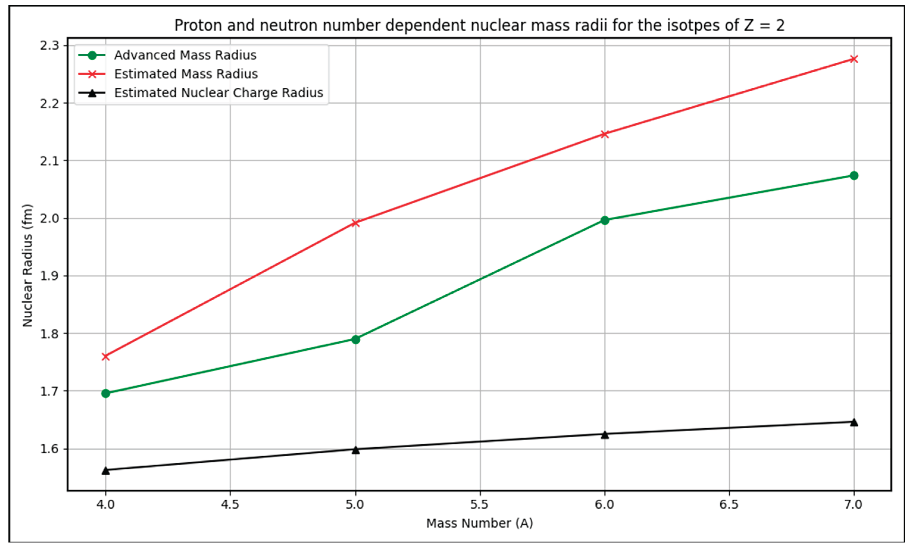
Figure 3.
Estimated mass radii of isotopes of Z=8 based on cubic root of proton and neutron numbers.
Figure 3.
Estimated mass radii of isotopes of Z=8 based on cubic root of proton and neutron numbers.
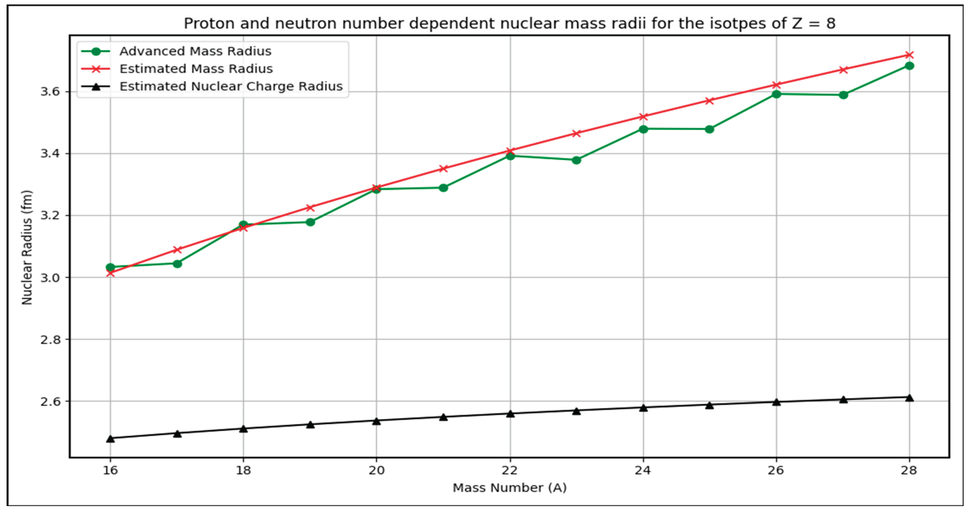
Figure 4.
Estimated mass radii of isotopes of Z=20 based on cubic root of proton and neutron numbers.
Figure 4.
Estimated mass radii of isotopes of Z=20 based on cubic root of proton and neutron numbers.
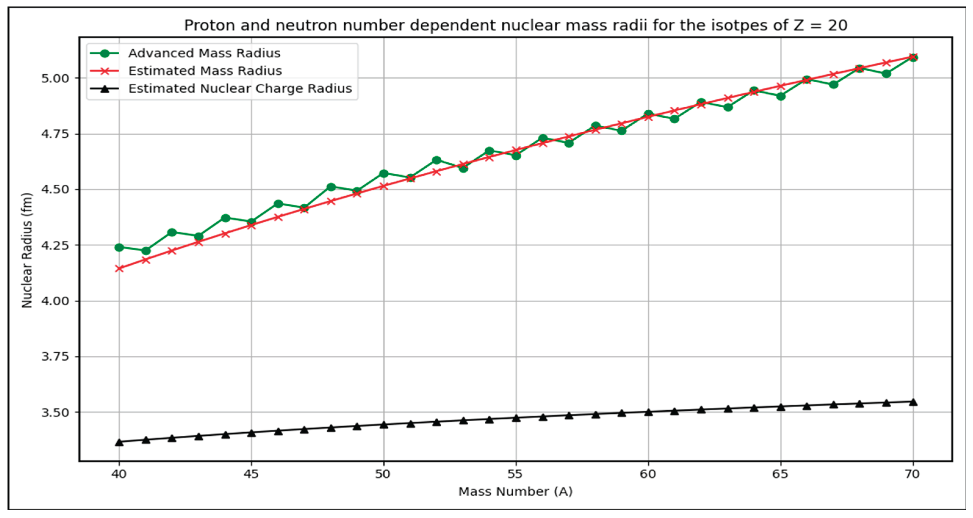
Figure 5.
Estimated mass radii of isotopes of Z=28 based on cubic root of proton and neutron numbers.
Figure 5.
Estimated mass radii of isotopes of Z=28 based on cubic root of proton and neutron numbers.
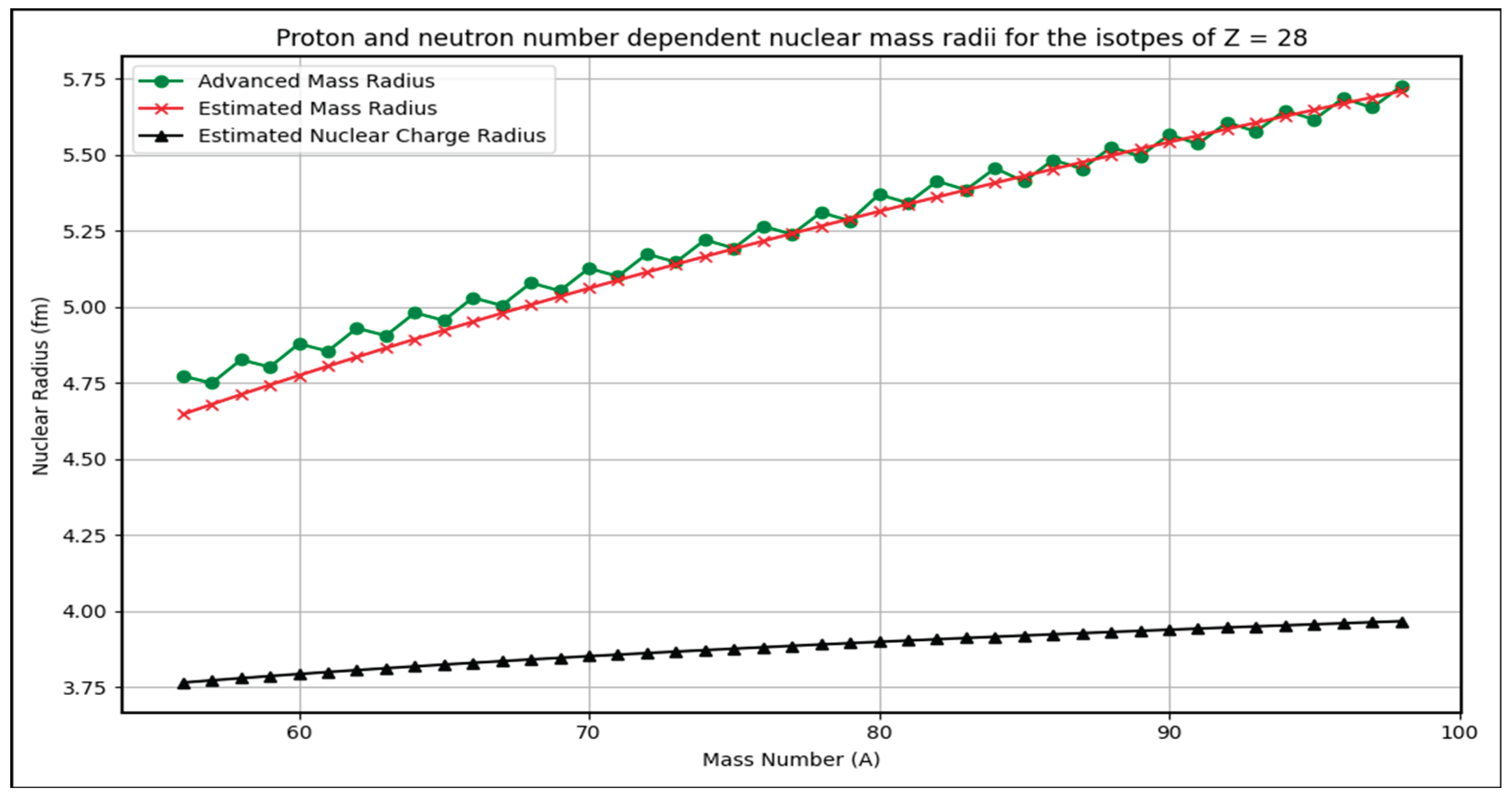
Figure 6.
Estimated mass radii of isotopes of Z=50 based on cubic root of proton and neutron numbers.
Figure 6.
Estimated mass radii of isotopes of Z=50 based on cubic root of proton and neutron numbers.
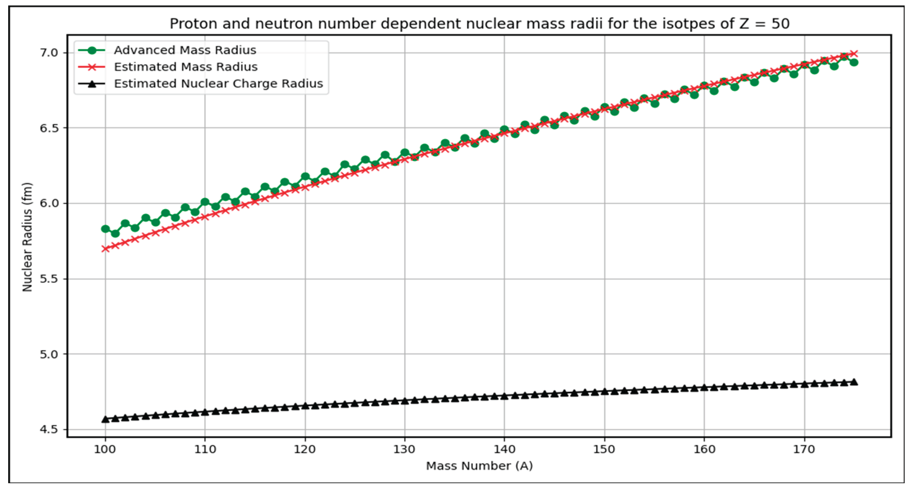
Figure 7.
Estimated mass radii of isotopes of Z=82 based on cubic root of proton and neutron numbers.
Figure 7.
Estimated mass radii of isotopes of Z=82 based on cubic root of proton and neutron numbers.
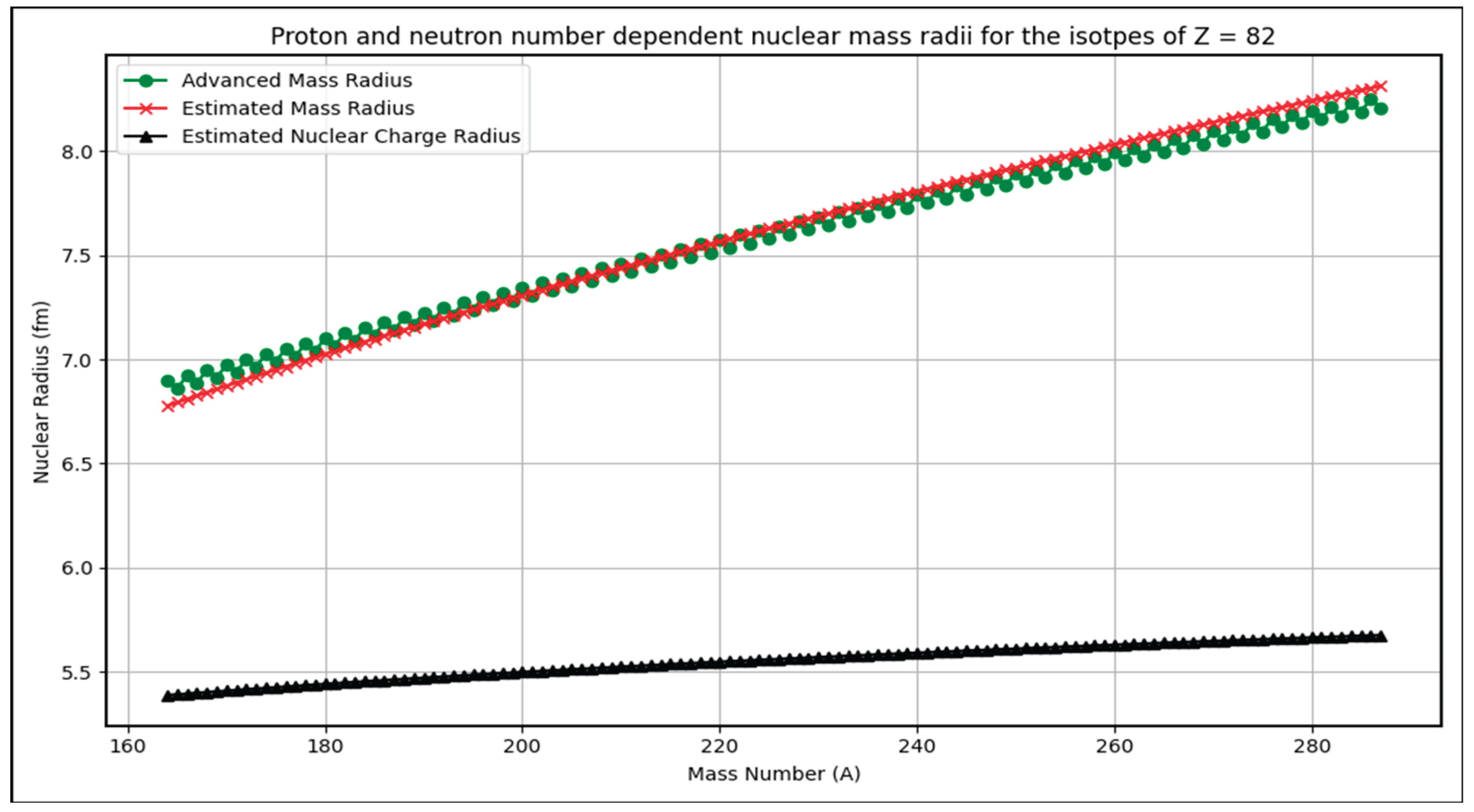
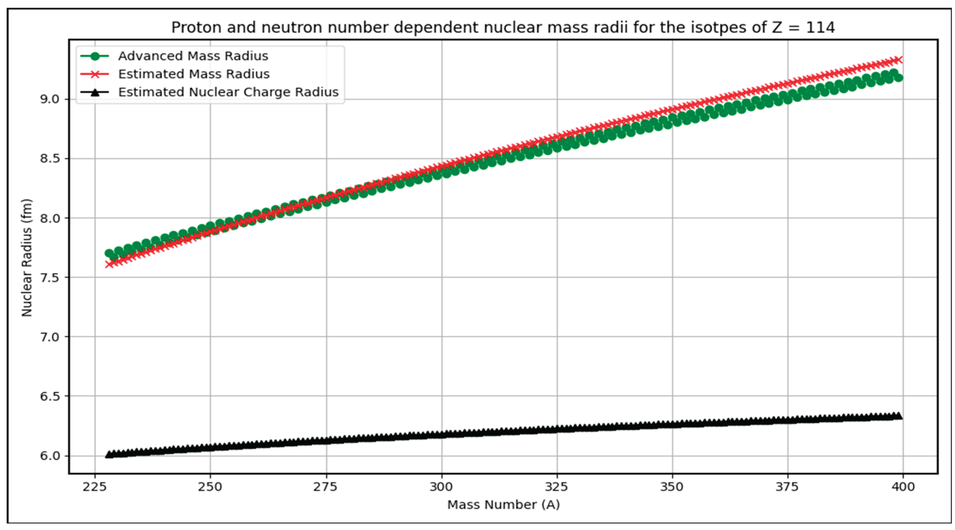
Figure 8.
Estimated mass radii of isotopes of Z=114 based on cubic root of proton and neutron numbers.
Figure 8.
Estimated mass radii of isotopes of Z=114 based on cubic root of proton and neutron numbers.
4.1. Data Table Observations and analysis
- (1)
- The table shows data for various nuclides with proton number (Z), neutron number (N), and mass number (A).
- (2)
- It lists the advanced radius, estimated nuclear charge radius (using relation involving Z1/3 and N1/3, mass distribution factor, estimated mass radius, and percentage error between the estimated and advanced mass radii.
- (3)
- The percentage error is generally very low, often below 2%, especially for medium and heavy nuclei. For example, for larger nuclei like Z=50 and above, errors hover near or below 1%, indicating high accuracy of the simple formula.
- (4)
- This confirms the simple formula’s efficacy for rapid nuclear radius estimation with minimal parameters, particularly suitable for large-scale or educational applications where complex calculations are impractical.
- (5)
- For Z=2 and its isotopes, average % error is 8.1%. Similarly for Z=8,20,28,50,82 and 114, average % errors are, 1.29%, 0.725%, 0.81%, 0.665%, 0.632% and 0.784% respectively. These percentage errors can be considered for further analysis positively.
- (6)
- Even though percentage errors are slightly larger (3 to 12 %) in very light nuclei, range of difference in radii is (0.03 to 0.14) fm. It needs further study.
4.2. Graphical Observations
- (1)
- The graphs depict estimated nuclear mass radii for isotopes of magic numbers Z=2, 8,20,28,50,82,114 as a function of mass number A.
- (2)
- Trends show a smooth increase in radius with increasing A, consistent with the power-law dependence on proton and neutron numbers.
- (3)
- The estimated radii closely track the advanced formula results across isotopes, validating the model’s predictive power.
- (4)
- Regions near magic numbers show slight structural effects possibly reflected in minor deviations or curvature in the radii trends.
The simple formula manages to capture these global trends well despite its simplicity, further supporting its practical utility.
4.3. Overall Commentary
The data table and accompanying graphs demonstrate that the proposed simple cubic-root-based formula with a tuneable mass distribution factor performs very well across a wide range of nuclei. It achieves accuracy comparable to more complex, parameter-heavy advanced formulas while offering significant simplicity in implementation. This balance makes it valuable for nuclear physics research, applications, and educational purposes focused on nuclear size estimation. Limitations are mainly restricted to very light nuclei where more detailed nuclear structure effects need consideration.
This strong agreement between experiment-based advanced formulas and the minimalistic approach underscores the 4G model’s foundational insight into nuclear size scaling using unified gravitational-electroweak parameters, serving as a promising theoretical tool.
5. Simplicity of the Proposed Formula
The minimalistic formula possesses several advantages:
- (1)
- It separately accounts for proton and neutron contributions through Z1/3 and N1/3, physically motivated by differing mass distributions.
- (2)
- The mass distribution coefficient Cmd introduces a tuneable mild dependence on proton number, neutron number and mass number offering empirical flexibility without excessive complication.
- (3)
- Compared to the multi-parameter advanced formula, it is computationally simpler and easier to implement in broad nuclear system studies or educational settings.
- (4)
- Despite its simplicity, it exhibits high fidelity across a broad mass range, supporting its utility for approximate radius calculations when detailed corrections are unavailable or unnecessary.
- (5)
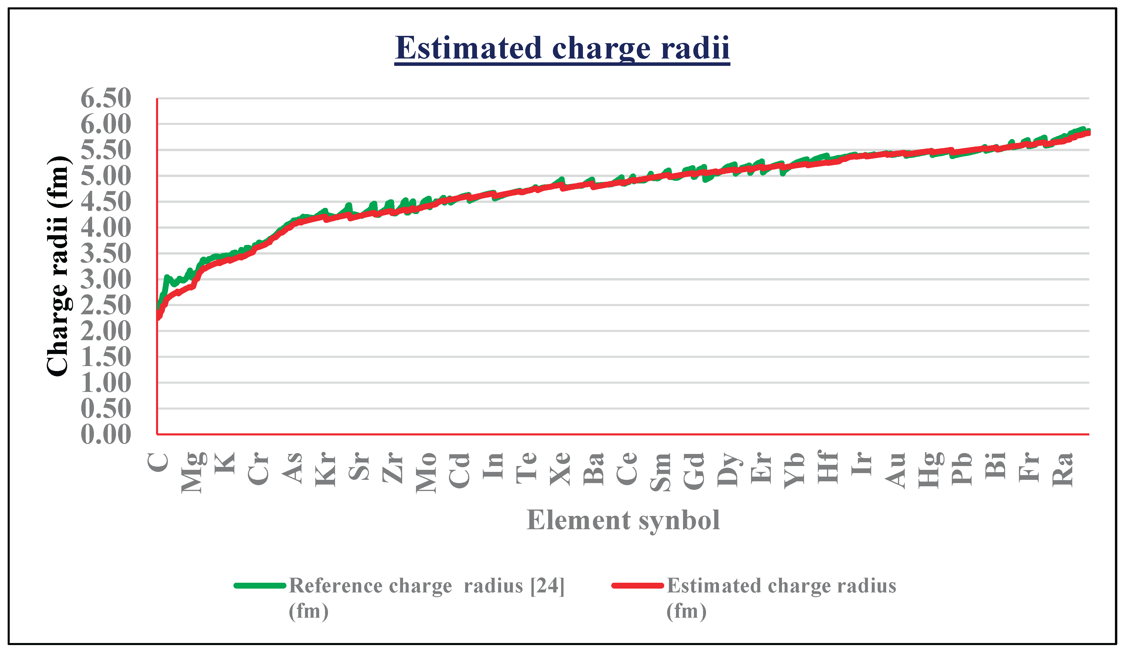
- Crucially, reliably approximates experimental nuclear charge radii [28,29,30,31] for a wide spectrum of elements. This strong correspondence validates the formula’s capability to capture essential aspects of nuclear spatial charge distribution, underscoring its scientific robustness and practical utility. See the following Figure 9 and Table 4. For light atomic nuclides, charge radius can be approximated with,
Figure 9.
Estimated charge radii of Z= (6 to 96) based on cubic root of proton and neutron numbers.
6. Python Program for Nuclear Mass Radius Calculation
This section provides a Python implementation of both the advanced nuclear radius formula and the proposed minimalistic formula incorporating the separate contributions of proton and neutron numbers with an empirical scaling factor. The program also calculates the percentage error between the two formulas to evaluate the accuracy of the simpler approach.
Proposed minimalistic formula reflects the intimate connection between nuclear structure and unified gravitational-electromagnetic interactions at the nuclear scale. It explicitly accounts for distinct mass distributions of protons and neutrons through terms Z1/3 and N1/3, providing a physically grounded representation of nuclear size. This approach, rooted in fundamental physics, demonstrates the 4G model’s potential for predictive power by bridging microscopic nuclear dimensions and universal constants.
| import math import csv import os import matplotlib.pyplot as plt def calculate_nuclear_radius_advanced(Z, A): N = A - Z I = (N - Z) / A if (Z % 2 == 0) and (N % 2 == 0): delta = 0 elif (Z % 2 == 1) and (N % 2 == 1): delta = 0.5 elif (Z % 2 == 1) and (N % 2 == 0): delta = 1 elif (Z % 2 == 0) and (N % 2 == 1): delta = -1 else: delta = 0 magic_numbers = [2, 8, 20, 28, 50, 82, 126] S = 0.1 if any(abs(A - m) <= 2 for m in magic_numbers) else 0 a = 1.25 b = -0.15 c = 0.05 d = -0.8 e = 0.2 f = 0.15 R = a * A ** (1/3) + b * I + c * delta + d * A ** (-1/3) + e + f * S return R # precision kept for calculations def calculate_estimated_radii(Z, A): N = A - Z estimated_charge_radius = 0.62 * (pow(Z,1/3)+pow(Z*Z*N,1/9)) sms = int((2 * Z) + (0.0064 * Z * Z)) mass_distribution_factor =1 + (pow(pow(Z*Z,0.5), 2/3) * 0.0073) + (0.1152*(1+pow((pow(N*N,0.5)-2)/A,0.5))) mass_distribution_factor =mass_distribution_factor*pow(A/sms,0.25) estimated_mass_radius = mass_distribution_factor * estimated_charge_radius return N, estimated_charge_radius, mass_distribution_factor, estimated_mass_radius def get_positive_integer(prompt): while True: try: value = int(input(prompt)) if value > 0: return value else: print("Please enter a positive integer greater than zero.") except ValueError: print("Invalid input. Please enter a positive integer.") def save_results_to_csv(Z, A_values, neutrons, advanced_radii, estimated_charge_radii, mass_distribution_factors, estimated_mass_radii, filename_csv): with open(filename_csv, mode='w', newline='') as file: writer = csv.writer(file) writer.writerow([ "Z", "N", "A", "Advanced Mass Radius (fm)", "Estimated Nuclear Charge Radius (fm)", "Mass Distribution Factor", "Estimated Mass Radius (fm)", "Percentage Error (%)" ]) error_sum = 0 count = 0 for i, A in enumerate(A_values): radius_adv = advanced_radii[i] radius_charge = estimated_charge_radii[i] mdf = mass_distribution_factors[i] radius_mass = estimated_mass_radii[i] neutron = neutrons[i] percent_error = abs((radius_mass - radius_adv) / radius_adv) * 100 writer.writerow([ Z, neutron, A, round(radius_adv, 4), round(radius_charge, 4), round(mdf, 5), round(radius_mass, 4), round(percent_error, 3) ]) error_sum += percent_error count += 1 avg_error = error_sum / count writer.writerow([]) writer.writerow(["Average % Error", "", "", "", "", "", "", round(avg_error, 3)]) print(f"Data has been saved to '{filename_csv}'.") def plot_nuclear_radii(Z, A_values, advanced_radii, estimated_charge_radii, estimated_mass_radii, filename_graph): fig, ax = plt.subplots(figsize=(10, 6)) ax.plot(A_values, advanced_radii, label='Advanced Mass Radius', marker='o', color='green') ax.plot(A_values, estimated_mass_radii, label='Estimated Mass Radius', marker='x', color='red') ax.plot(A_values, estimated_charge_radii, label='Estimated Nuclear Charge Radius', marker='^', color='black') ax.set_xlabel('Mass Number (A)') ax.set_ylabel('Nuclear Radius (fm)') ax.set_title(f'Proton and neutron number dependent nuclear mass radii for the isotpes of Z = {Z}') ax.legend() ax.grid(True) # Set border thickness for all four axis spines for spine in ax.spines.values(): spine.set_linewidth(1.5) # Add border around entire figure fig.patch.set_linewidth(2) fig.patch.set_edgecolor('black') fig.patch.set_facecolor('white') # Keep background white plt.tight_layout() plt.savefig(filename_graph) print(f"Graph has been saved as '{filename_graph}'.") plt.show() def main(): print("Current working directory:", os.getcwd()) Z = get_positive_integer("Enter proton number Z: ") A_lower = 2 * Z A_upper = int(3.5 * Z) A_values = list(range(A_lower, A_upper + 1)) neutrons = [] advanced_radii = [] estimated_charge_radii = [] mass_distribution_factors = [] estimated_mass_radii = [] for A in A_values: N, charge_r, mdf, mass_r = calculate_estimated_radii(Z, A) neutrons.append(N) estimated_charge_radii.append(charge_r) mass_distribution_factors.append(mdf) estimated_mass_radii.append(mass_r) advanced_radii.append(calculate_nuclear_radius_advanced(Z, A)) filename_csv = f"nuclear_radius_output_Z{Z}.csv" filename_graph = f"nuclear_radius_plot_Z{Z}.png" save_results_to_csv(Z, A_values, neutrons, advanced_radii, estimated_charge_radii, mass_distribution_factors, estimated_mass_radii, filename_csv) plot_nuclear_radii(Z, A_values, advanced_radii, estimated_charge_radii, estimated_mass_radii, filename_graph) if __name__ == "__main__": main() |
7. Discussion
The present study introduces a simplified yet physically insightful formula for estimating nuclear mass and charge radii, founded on the 4G model of final unification. This model fundamentally distinguishes itself by emphasizing the distinct contributions of protons and neutrons to the nuclear radius through separate cubic root dependencies, Z1/3 and N1/3. This separation aligns with the physical reality that protons and neutrons have different spatial distributions and roles within the nucleus due to their differing charges, masses, and interactions.
7.1. Physical Rationale for Separate Contributions
Traditional empirical formulas often treat the nucleus as a single entity characterized by the mass number A=Z+N. However, nuclear structure details—such as proton-neutron asymmetry, shell effects, and pairing correlations—play a pivotal role in defining size and shape. Incorporating separate proton and neutron terms allows nuanced capture of mass distribution asymmetries, especially significant in nuclei far from stability or near magic numbers. This feature explains why the proposed formula maintains respectable accuracy even for nuclei exhibiting moderate isospin imbalance or structural complexities, without resorting to a large number of empirical parameters.
7.2. Role of the Mass Distribution Coefficient
The introduction of the proton-number-dependent mass distribution coefficient Cmd is a crucial enhancement, providing empirical flexibility to the model. It fine-tunes the overall radial scale in a manner reflecting changes in spatial distribution associated with increasing proton numbers starting from Z=(2 to 118). This approach encapsulates subtle structural shifts such as deformation and changes in density profiles, which manifest more evidently in heavier nuclei. By avoiding highly complex functional forms or excessive fitting parameters, the model achieves a balanced trade-off between simplicity and precision.
7.3. Accuracy and Limitations Across the Nuclear Chart
Benchmarking results show the simplified formula competes well with advanced formulas that include multiple correction terms for isospin asymmetry, shell closure effects, and odd-even staggering. The percent error remains generally under 2% for medium to heavy nuclei, underscoring the model's robustness and practical utility in nuclear physics applications demanding fast and reasonably accurate radius estimates.
However, as is typical for simplistic power-law approximations, the model exhibits larger deviations in very light nuclei (e.g., 4He), where quantum effects, cluster structures, and strong pairing correlations dominate spatial characteristics beyond mere mass scaling. This recognition invites further refinement or complementary modelling efforts to address these special cases.
7.4. Implications for Nuclear Modelling and Astrophysical Phenomena
Accurate nuclear radius estimation is critical for diverse fields including nuclear reaction modelling, astrophysical nucleosynthesis, and neutron star matter characterization. The 4G model’s simplicity facilitates incorporation into computational frameworks, Monte Carlo simulations, and educational tools where computational efficiency is prized. Its grounding in unified interaction scales, tying nuclear size parameters to fundamental constants and coupling strengths, may yield novel insights into the interplay between nuclear microphysics and overarching fundamental forces.
7.5. Connection to Fundamental Constants
By linking the mass radius scaling to electroweak and large gravitational coupling constants, the model hints at a deeper unification of nuclear dimensions with universal physical constants. This perspective aligns with ongoing efforts in theoretical physics to connect quantum mechanical scales with cosmological and gravitational phenomena, potentially bridging gaps in understanding nuclear matter across scales.
7.6. Limitations, Outlook and Future Directions
A) Limitations and Open Questions
- (1)
- Light Nuclei Accuracy: For light nuclei (e.g., Helium-4), the simplified formula cannot accommodate quantum effects, cluster structures, or strong pairing correlations captured by detailed advanced models; errors rise above 5–10% in some cases.
- (2)
- Physical Basis for Mass Distribution Coefficient: The mass distribution factor Cmd is currently tuned with fine structure ratio and the strong coupling constant. Even though there is limited discussion on its theoretical underpinnings—further studies or density functional theory analyses might clarify its physical interpretation.
- (3)
- Neglect of Higher Order Corrections: While the formula’s simplicity is a virtue, effects such as deformation, nuclear skin thickness, or isospin-dependent density variations are only indirectly and approximately encoded.
B) Outlook and Future Directions
The encouraging results prompt several avenues for enhancement and exploration. Incorporating deformation-dependent corrections or pairing-gap influences without sacrificing simplicity could extend accuracy to light and deformed nuclei. Further empirical analyses across isotopic chains near drip lines would clarify model robustness under extreme conditions. Moreover, exploring theoretical foundations of the mass distribution coefficient in the context of nuclear density functional theory or ab initio calculations could provide firmer physical interpretation and predictive capabilities.
Overall, this discussion highlights that the presented 4G-based nuclear radius formula offers a promising framework that respects the nuanced roles of proton and neutron distributions while maintaining usable simplicity. It stands as a practical tool for rapid nuclear size estimation with solid physical relevance and potential for integration into broader nuclear and astrophysical modelling landscapes.
The advanced nuclear mass radius formula coefficients a,b,c,d,e,f indeed vary due to differing datasets and fitting approaches, making a unique or standardized set elusive. Our outlined uncertainty ranges for these coefficients reflect realistic parameter sensitivities and provide valuable guidance for robustness testing or refined empirical fits:
Coefficient, a =1.25 and its range, 1.1875 to 1.3125
Coefficient, b = -0.15 and its range, -0.1575 to -0.1425
Coefficient, c =0.05 and its range, 0.0475 to 0.0525
Coefficient, d = -0.8 and its range, -0.84 to -0.76
Coefficient, e = 0.2 and its range, 0.19 to 0.21
Coefficient, f = 0.15 and its range, 0.1425 to 0.1575
This explicit representation of coefficient variability facilitates more transparent sensitivity analyses and refinement efforts in nuclear mass radius modelling, addressing the non-uniqueness concerns in empirical approaches.
Simultaneously, our proposed simplified 4G model-based formula incorporating:
- Separate proton (Z1/3) and neutron (N1/3) contributions,
- A physically motivated, tuneable mass distribution coefficient (Cmd) linked to fundamental constants (fine structure ratio, strong coupling constant),
- Minimal adjustable parameters compared to multi-coefficient advanced formulas,
provides a compelling alternative framework. It achieves comparable accuracy across medium to heavy nuclei with reduced complexity and increased physical transparency. This approach shifts focus from fine-tuning within a non-unique parameter space to grounding radius estimation in unified interaction scales, enhancing theoretical consistency and practical usability.
The bibliographic references of this paper reinforce these insights by offering a wide foundation of experimental and theoretical nuclear radius data, model variations, and related nuclear physics fundamentals. These can be used for further validation and contextualization of coefficient ranges and formula applicability.
Thus,
- The advanced formula coefficients are best applied acknowledging typical ±5% variability or uncertainty.
- The 4G model’s simplified formula stands as a robust, physically transparent, and practical nuclear radius estimation method, reducing reliance on complex empirical parameter calibrations.
- This dual perspective—combining empirical coefficient sensitivity awareness and physically motivated simplification—provides a comprehensive, precise, and efficient framework for nuclear radius evaluations in both academic and applied contexts.
This presentation style—clarifying coefficient uncertainties alongside physically based model advantages—can indeed improve precision and usability throughout related academic and practical documents on nuclear mass and charge radii estimation.
8. Conclusion
This study presents a simple and physically motivated formula for estimating nuclear radii that effectively balances minimal parameterization with reasonable accuracy. By explicitly incorporating the separate contributions of proton and neutron numbers through cubic-root dependencies and introducing a mass distribution coefficient of the form (1+ x + y) assumed to be associated with fine structure ratio and strong coupling constant, the formula achieves excellent agreement with an advanced nuclear radius formula that includes detailed nuclear structure corrections.
The proposed formula’s simplicity enables rapid and transparent nuclear radius estimations, making it particularly valuable for applications where computational efficiency and clear physical interpretation are essential. It provides a practical alternative for nuclear physics research and education, facilitating studies across a broad range of nuclei without requiring complex fitting parameters.
While the formula is highly reliable for medium to heavy nuclei, limitations exist for very light nuclei where effects such as pairing, deformation, and clustering play a significant role and are not captured by simple power laws. Future work may focus on refining the scaling factors or incorporating additional physical effects to enhance accuracy for these cases.
Overall, the approach exemplifies the potential of the 4G model of final unification to unify nuclear structural properties with universal fundamental constants, supporting its role as a valuable tool for efficient and insightful nuclear radius estimation.
Data Availability Statement
The data that support the findings of this study are openly available.
Acknowledgements
Author Seshavatharam is indebted to professors Padma Shri M. Nagaphani Sarma, Chairman, Shri K.V. Krishna Murthy, founder Chairman, Institute of Scientific Research in Vedas (ISERVE), Hyderabad, India and Shri K.V.R.S. Murthy, former scientist IICT (CSIR), Govt. of India, Director, Research and Development, I-SERVE, for their valuable guidance and great support in developing this subject. Author is very much thankful to AI for a useful discussion and guidance.
Conflict of Interest
Authors declare no conflict of interest in this paper or subject.
References
- Rutherford, E. The scattering of α and β particles by matter and the structure of the atom. Philosophical Magazine, 21(125), 669-688, 1911.
- N. Gauthier; Deriving a formula for nuclear radii using the measured atomic masses of elements. Am. J. Phys. 57 (4): 344–346, 1989. [CrossRef]
- Nerlo-Pomorska, B., Pomorski, K. Simple formula for nuclear charge radius. Z. Physik A - Hadrons and Nuclei. 348, 169–172, 1994. [CrossRef]
- Hiroyuki Koura, Masahiro Unoa, Takahiro Tachibana, Masami Yamadaa. Nuclear mass formula with shell energies calculated by a new method. Nuclear Physics A 674. 47–76, 2000. [CrossRef]
- Möller, P., Nix, J.R., Myers, W.D., Swiatecki, W.J., Nuclear Ground-State Masses and Deformations, Atomic Data and Nuclear Data Tables 59, 185–381 (1995). [CrossRef]
- Audi, G., Wang, M., Wapstra, A.H., et al., The Ame2012 Atomic Mass Evaluation: (II). Tables, Graphs, and References, Chinese Physics C, 36(12), 1287–1602 (2012).
- Brown, B.A., Proton and neutron radii in nuclei, Phys. Rev. Lett. 85, 5296–5299 (2000).
- Yao, J.M., et al. Constraints on nuclear symmetry energy and neutron skins from nuclear collective oscillations, Frontiers in Physics 8, Article 55 (2020).
- Seshavatharam U. V. S, Gunavardhana Naidu T and Lakshminarayana S. Nuclear evidences for confirming the physical existence of 585 GeV weak fermion and galactic observations of TeV radiation. International Journal of Advanced Astronomy. 13(1):1-17, 2025.
- Seshavatharam U V S and Lakshminarayana S. 4G model of final unification – A brief report Journal of Physics: Conference Series 2197 p 012029, 2022.
- Seshavatharam U.V.S and Lakshminarayana S. A very brief review on strong and electroweak mass formula pertaining to 4G model of final unification. Proceedings of the DAE Symp. on Nucl. Phys. 67,1173, 2023.
- Apoorva D. Patel. EPR Paradox, Bell Inequalities and Peculiarities of Quantum Correlations.arXiv:2502.06791v1,2025. [CrossRef]
- Clifford Cheung, Aaron Hillman, Grant N. Remmen. String Theory May Be Inevitable as a Unified Theory of Physics. Physics World, 2025.
- Ahmed Abokhalil. The Higgs Mechanism and Higgs Boson: Unveiling the Symmetry of the Universe. arXiv:2306.01019v2 [hep-ph].
- Koura, H., Uno, M., Tachibana, T., & Yamada, M. Nuclidic mass formula with shell and pairing corrections. Nucl. Phys. A 674, 47–70. 2005.
- LI Ru-Heng, HU Yong-Mao and LI Mao-Cai. An analysis of nuclear charge radii based on the empirical formula.CPC(HEP & NP), 33(Suppl.): 123—125 C, 2009. [CrossRef]
- Lu Tang and Zhen-Hua Zhang. Nuclear charge radius predictions by kernel ridge regression with odd-even effects. Nucl. Sci. Tech. 35, 19, 2024. [CrossRef]
- Tuncay Bayram, Serkan Akkoyun, S.Okan Kara, Alper Sinan. New Parameters for Nuclear Charge Radius Formulas. Acta Phys. Polon.B 44, 8, 1791-1799,2013. [CrossRef]
- Y.H. Wang, D.Y. Pang, W.D. Chen, Y.P. Xu, W.L. Hai. Nuclear radii from total reaction cross section measurements at intermediate energies with complex turning point corrections to the eikonal model.Phys.Rev.C 109, 1, 014621, 2024. [CrossRef]
- Takayuki Miyagi. Nuclear radii from first principles. Front. Phys., 09 May 2025. [CrossRef]
- S. Navas et al. Electroweak Model and Constraints on New Physics.
- S. Navas et al. Quantum Chromodynamics. (Particle Data Group), Phys. Rev. D 110, 030001, 2024.
- D d’Enterria et al. The strong coupling constant: state of the art and the decade ahead. J. Phys. G: Nucl. Part. Phys. 51 090501, 2024. [CrossRef]
- Seshavatharam U.V.S and Lakshminarayana S. Computing unified atomic mass unit and Avogadro number with various nuclear binding energy formulae coded in Python. Int. J. Chem. Stud. 2025;13(1):24-30.
- Seshavatharam, U. V. S.; Lakshminarayana, S. Revised Electroweak and Asymmetry Terms of the Strong and Electroweak Mass Formula Associated with 4G Model of Final Unification. Preprints 2025050425, 2025.
- P.R. Chowdhury, C. Samanta, D.N. Basu, Modified Bethe– Weizsacker mass formula with isotonic shift and new driplines. Mod. Phys. Lett. A 20, 1605–1618, 2005.
- G. Royer, On the coefficients of the liquid drop model mass formulae and nuclear radii. Nuclear Physics A, 807, 3–4, 105-118, 2008. [CrossRef]
- I. Angeli, K.P. Marinova, Table of experimental nuclear ground state charge radii: An update, Atomic Data and Nuclear Data Tables 99, 69–95, 2013. [CrossRef]
- Ning Wang and Tao Li. Shell and isospin effects in nuclear charge radii.Phys. Rev. C 88, 011301(R). [CrossRef]
- Rong An, Xiang Jiang, Na Tang, Li-Gang Cao, Feng-Shou Zhang. An improved description of nuclear charge radii: Global trends beyond N = 28 shell closure.arXiv:2312.04912v1 [nucl-th], 2024.
- Tao Li, Yani Luo, Ning Wang, Compilation of recent nuclear ground state charge radius measurements and tests for models, Atomic Data and Nuclear Data Tables, 140, 2021. [CrossRef]
Figure 1.
Estimated mass radii of Z=2 to 118 based on proton and neutron numbers.
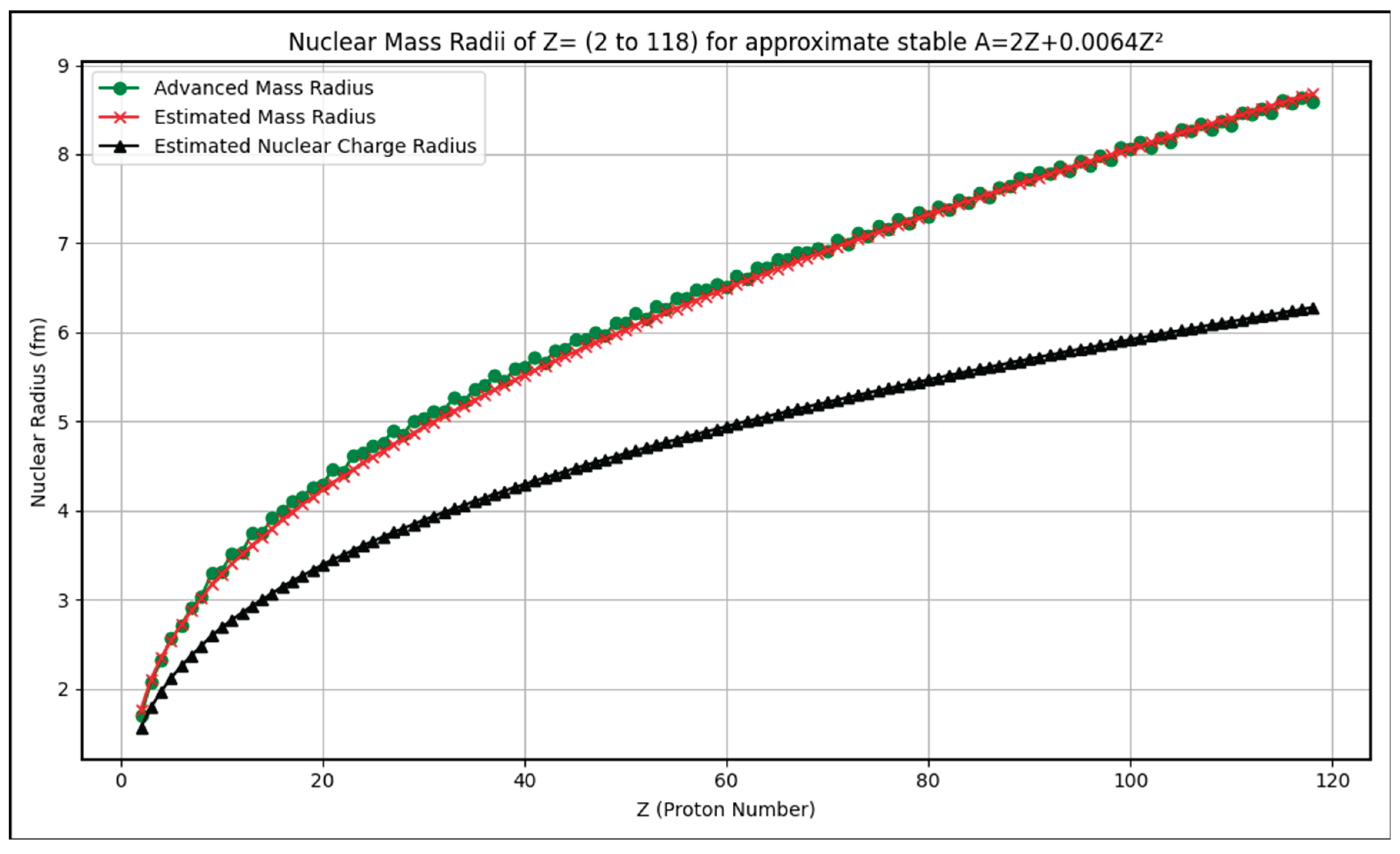
Table 1.
Charge dependent string tensions and string energies.
| S.No | Interaction | String Tension | String Energy |
|---|---|---|---|
|
1 |
Weak |
||
|
2 |
Strong |
||
|
3 |
Electromagnetic |
Table 2.
Quantum string tensions and string energies.
| S.No | Interaction | String Tension | String Energy |
|---|---|---|---|
|
1 |
Weak |
||
|
2 |
Strong |
||
|
3 |
Electromagnetic |
Table 4.
Estimated nuclear charge radii.
| Symbol | Z | N | Approximate Stable Mass Number As | Reference Charge Radius [24] (fm) |
Reference Uncertainty (fm) | Estimated Charge Radius (fm) | Difference (fm) |
%Error |
|---|---|---|---|---|---|---|---|---|
| C | 6 | 6 | 12 | 2.4702 | 0.0022 | 2.2532 | 0.2170 | 8.78 |
| C | 6 | 7 | 13 | 2.4614 | 0.0034 | 2.2727 | 0.1887 | 7.67 |
| C | 6 | 8 | 14 | 2.5025 | 0.0087 | 2.2898 | 0.2127 | 8.50 |
| N | 7 | 7 | 14 | 2.5582 | 0.007 | 2.3720 | 0.1862 | 7.28 |
| N | 7 | 8 | 15 | 2.6058 | 0.008 | 2.3898 | 0.2160 | 8.29 |
| O | 8 | 8 | 16 | 2.6991 | 0.0052 | 2.4800 | 0.2191 | 8.12 |
| O | 8 | 9 | 17 | 2.6932 | 0.0075 | 2.4963 | 0.1969 | 7.31 |
| O | 8 | 10 | 18 | 2.7726 | 0.0056 | 2.5111 | 0.2615 | 9.43 |
| F | 9 | 10 | 19 | 2.8976 | 0.0025 | 2.5945 | 0.3031 | 10.46 |
| Ne | 10 | 7 | 17 | 3.0413 | 0.0088 | 2.6196 | 0.4217 | 13.87 |
| Ne | 10 | 8 | 18 | 2.9714 | 0.0076 | 2.6388 | 0.3326 | 11.19 |
| Ne | 10 | 9 | 19 | 3.0082 | 0.004 | 2.6560 | 0.3522 | 11.71 |
| Ne | 10 | 10 | 20 | 3.0055 | 0.0021 | 2.6715 | 0.3340 | 11.11 |
| Ne | 10 | 11 | 21 | 2.9695 | 0.0033 | 2.6857 | 0.2838 | 9.56 |
| Ne | 10 | 12 | 22 | 2.9525 | 0.004 | 2.6988 | 0.2537 | 8.59 |
| Ne | 10 | 13 | 23 | 2.9104 | 0.0071 | 2.7110 | 0.1994 | 6.85 |
| Ne | 10 | 14 | 24 | 2.9007 | 0.0078 | 2.7224 | 0.1783 | 6.15 |
| Ne | 10 | 15 | 25 | 2.9316 | 0.0088 | 2.7331 | 0.1985 | 6.77 |
| Ne | 10 | 16 | 26 | 2.9251 | 0.01 | 2.7431 | 0.1820 | 6.22 |
| Ne | 10 | 18 | 28 | 2.9642 | 0.0134 | 2.7616 | 0.2026 | 6.83 |
| Na | 11 | 9 | 20 | 2.9718 | 0.042 | 2.7273 | 0.2445 | 8.23 |
| Na | 11 | 10 | 21 | 3.0136 | 0.0284 | 2.7432 | 0.2704 | 8.97 |
| Na | 11 | 11 | 22 | 2.9852 | 0.0169 | 2.7577 | 0.2275 | 7.62 |
| Na | 11 | 12 | 23 | 2.9936 | 0.0021 | 2.7711 | 0.2225 | 7.43 |
| Na | 11 | 13 | 24 | 2.9735 | 0.0169 | 2.7836 | 0.1899 | 6.39 |
| Na | 11 | 14 | 25 | 2.9769 | 0.0252 | 2.7952 | 0.1817 | 6.10 |
| Na | 11 | 15 | 26 | 2.9928 | 0.0331 | 2.8061 | 0.1867 | 6.24 |
| Na | 11 | 16 | 27 | 3.0136 | 0.0467 | 2.8164 | 0.1972 | 6.55 |
| Na | 11 | 17 | 28 | 3.04 | 0.0581 | 2.8261 | 0.2139 | 7.04 |
| Na | 11 | 18 | 29 | 3.0922 | 0.0723 | 2.8353 | 0.2569 | 8.31 |
| Na | 11 | 19 | 30 | 3.118 | 0.0884 | 2.8441 | 0.2739 | 8.79 |
| Na | 11 | 20 | 31 | 3.1704 | 0.0893 | 2.8524 | 0.3180 | 10.03 |
| Mg | 12 | 12 | 24 | 3.057 | 0.0016 | 2.8389 | 0.2181 | 7.13 |
| Mg | 12 | 13 | 25 | 3.0284 | 0.0022 | 2.8516 | 0.1768 | 5.84 |
| Mg | 12 | 14 | 26 | 3.0337 | 0.0018 | 2.8634 | 0.1703 | 5.61 |
| Al | 13 | 14 | 27 | 3.061 | 0.0031 | 2.9277 | 0.1333 | 4.35 |
| Si | 14 | 14 | 28 | 3.1224 | 0.0024 | 2.9886 | 0.1338 | 4.29 |
| Si | 14 | 15 | 29 | 3.1176 | 0.0052 | 3.0001 | 0.1175 | 3.77 |
| Si | 14 | 16 | 30 | 3.1336 | 0.004 | 3.0109 | 0.1227 | 3.92 |
| P | 15 | 16 | 31 | 3.1889 | 0.0019 | 3.0691 | 0.1198 | 3.76 |
| S | 16 | 16 | 32 | 3.2611 | 0.0018 | 3.1246 | 0.1365 | 4.19 |
| S | 16 | 18 | 34 | 3.2847 | 0.0021 | 3.1452 | 0.1395 | 4.25 |
| S | 16 | 20 | 36 | 3.2985 | 0.0024 | 3.1638 | 0.1347 | 4.08 |
| Cl | 17 | 18 | 35 | 3.3654 | 0.0191 | 3.1985 | 0.1669 | 4.96 |
| Cl | 17 | 20 | 37 | 3.384 | 0.017 | 3.2174 | 0.1666 | 4.92 |
| Ar | 18 | 14 | 32 | 3.3468 | 0.0062 | 3.2050 | 0.1418 | 4.24 |
| Ar | 18 | 15 | 33 | 3.3438 | 0.0058 | 3.2171 | 0.1267 | 3.79 |
| Ar | 18 | 16 | 34 | 3.3654 | 0.004 | 3.2286 | 0.1368 | 4.07 |
| Ar | 18 | 17 | 35 | 3.3636 | 0.0042 | 3.2394 | 0.1242 | 3.69 |
| Ar | 18 | 18 | 36 | 3.3905 | 0.0023 | 3.2497 | 0.1408 | 4.15 |
| Ar | 18 | 19 | 37 | 3.3908 | 0.0022 | 3.2595 | 0.1313 | 3.87 |
| Ar | 18 | 20 | 38 | 3.4028 | 0.0019 | 3.2689 | 0.1339 | 3.94 |
| Ar | 18 | 21 | 39 | 3.4093 | 0.0031 | 3.2778 | 0.1315 | 3.86 |
| Ar | 18 | 22 | 40 | 3.4274 | 0.0026 | 3.2864 | 0.1410 | 4.12 |
| Ar | 18 | 23 | 41 | 3.4251 | 0.003 | 3.2946 | 0.1305 | 3.81 |
| Ar | 18 | 24 | 42 | 3.4414 | 0.0041 | 3.3025 | 0.1389 | 4.04 |
| Ar | 18 | 25 | 43 | 3.4354 | 0.0039 | 3.3101 | 0.1253 | 3.65 |
| Ar | 18 | 26 | 44 | 3.4454 | 0.0046 | 3.3175 | 0.1279 | 3.71 |
| Ar | 18 | 28 | 46 | 3.4377 | 0.0044 | 3.3315 | 0.1062 | 3.09 |
| K | 19 | 19 | 38 | 3.4264 | 0.0051 | 3.3088 | 0.1176 | 3.43 |
| K | 19 | 20 | 39 | 3.4349 | 0.0019 | 3.3183 | 0.1166 | 3.40 |
| K | 19 | 21 | 40 | 3.4381 | 0.0028 | 3.3273 | 0.1108 | 3.22 |
| K | 19 | 22 | 41 | 3.4518 | 0.0055 | 3.3360 | 0.1158 | 3.36 |
| K | 19 | 23 | 42 | 3.4517 | 0.007 | 3.3443 | 0.1074 | 3.11 |
| K | 19 | 24 | 43 | 3.4556 | 0.0086 | 3.3523 | 0.1033 | 2.99 |
| K | 19 | 25 | 44 | 3.4563 | 0.0101 | 3.3600 | 0.0963 | 2.78 |
| K | 19 | 26 | 45 | 3.4605 | 0.0118 | 3.3675 | 0.0930 | 2.69 |
| K | 19 | 27 | 46 | 3.4558 | 0.0126 | 3.3747 | 0.0811 | 2.35 |
| K | 19 | 28 | 47 | 3.4534 | 0.0138 | 3.3817 | 0.0717 | 2.08 |
| Ca | 20 | 19 | 39 | 3.4595 | 0.0025 | 3.3563 | 0.1032 | 2.98 |
| Ca | 20 | 20 | 40 | 3.4776 | 0.0019 | 3.3659 | 0.1117 | 3.21 |
| Ca | 20 | 21 | 41 | 3.478 | 0.0019 | 3.3750 | 0.1030 | 2.96 |
| Ca | 20 | 22 | 42 | 3.5081 | 0.0021 | 3.3838 | 0.1243 | 3.54 |
| Ca | 20 | 23 | 43 | 3.4954 | 0.0019 | 3.3922 | 0.1032 | 2.95 |
| Ca | 20 | 24 | 44 | 3.5179 | 0.0021 | 3.4003 | 0.1176 | 3.34 |
| Ca | 20 | 25 | 45 | 3.4944 | 0.0021 | 3.4081 | 0.0863 | 2.47 |
| Ca | 20 | 26 | 46 | 3.4953 | 0.002 | 3.4157 | 0.0796 | 2.28 |
| Ca | 20 | 27 | 47 | 3.4783 | 0.0024 | 3.4229 | 0.0554 | 1.59 |
| Ca | 20 | 28 | 48 | 3.4771 | 0.002 | 3.4300 | 0.0471 | 1.35 |
| Ca | 20 | 30 | 50 | 3.5168 | 0.0064 | 3.4434 | 0.0734 | 2.09 |
| Sc | 21 | 21 | 42 | 3.5702 | 0.0238 | 3.4211 | 0.1491 | 4.18 |
| Sc | 21 | 22 | 43 | 3.5575 | 0.0147 | 3.4299 | 0.1276 | 3.59 |
| Sc | 21 | 23 | 44 | 3.5432 | 0.0016 | 3.4384 | 0.1048 | 2.96 |
| Sc | 21 | 24 | 45 | 3.5459 | 0.0025 | 3.4466 | 0.0993 | 2.80 |
| Sc | 21 | 25 | 46 | 3.5243 | 0.0089 | 3.4545 | 0.0698 | 1.98 |
| Ti | 22 | 22 | 44 | 3.6115 | 0.0051 | 3.4745 | 0.1370 | 3.79 |
| Ti | 22 | 23 | 45 | 3.5939 | 0.0032 | 3.4831 | 0.1108 | 3.08 |
| Ti | 22 | 24 | 46 | 3.607 | 0.0022 | 3.4914 | 0.1156 | 3.20 |
| Ti | 22 | 25 | 47 | 3.5962 | 0.0019 | 3.4994 | 0.0968 | 2.69 |
| Ti | 22 | 26 | 48 | 3.5921 | 0.0017 | 3.5071 | 0.0850 | 2.37 |
| Ti | 22 | 27 | 49 | 3.5733 | 0.0021 | 3.5145 | 0.0588 | 1.65 |
| Ti | 22 | 28 | 50 | 3.5704 | 0.0022 | 3.5217 | 0.0487 | 1.36 |
| V | 23 | 28 | 51 | 3.6002 | 0.0022 | 3.5654 | 0.0348 | 0.97 |
| Cr | 24 | 26 | 50 | 3.6588 | 0.0065 | 3.5928 | 0.0660 | 1.81 |
| Cr | 24 | 28 | 52 | 3.6452 | 0.0042 | 3.6077 | 0.0375 | 1.03 |
| Cr | 24 | 29 | 53 | 3.6511 | 0.0075 | 3.6148 | 0.0363 | 0.99 |
| Cr | 24 | 30 | 54 | 3.6885 | 0.0074 | 3.6217 | 0.0668 | 1.81 |
| Mn | 25 | 25 | 50 | 3.712 | 0.0196 | 3.6258 | 0.0862 | 2.32 |
| Mn | 25 | 26 | 51 | 3.7026 | 0.0212 | 3.6337 | 0.0689 | 1.86 |
| Mn | 25 | 27 | 52 | 3.6706 | 0.0128 | 3.6414 | 0.0292 | 0.80 |
| Mn | 25 | 28 | 53 | 3.6662 | 0.0076 | 3.6488 | 0.0174 | 0.48 |
| Mn | 25 | 29 | 54 | 3.6834 | 0.0049 | 3.6559 | 0.0275 | 0.75 |
| Mn | 25 | 30 | 55 | 3.7057 | 0.0022 | 3.6629 | 0.0428 | 1.16 |
| Mn | 25 | 31 | 56 | 3.7146 | 0.0052 | 3.6696 | 0.0450 | 1.21 |
| Fe | 26 | 28 | 54 | 3.6933 | 0.0019 | 3.6887 | 0.0046 | 0.13 |
| Fe | 26 | 30 | 56 | 3.7377 | 0.0016 | 3.7029 | 0.0348 | 0.93 |
| Fe | 26 | 31 | 57 | 3.7532 | 0.0017 | 3.7097 | 0.0435 | 1.16 |
| Fe | 26 | 32 | 58 | 3.7745 | 0.0014 | 3.7164 | 0.0581 | 1.54 |
| Co | 27 | 32 | 59 | 3.7875 | 0.0021 | 3.7554 | 0.0321 | 0.85 |
| Ni | 28 | 30 | 58 | 3.7757 | 0.002 | 3.7799 | -0.0042 | -0.11 |
| Ni | 28 | 32 | 60 | 3.8118 | 0.0016 | 3.7935 | 0.0183 | 0.48 |
| Ni | 28 | 33 | 61 | 3.8225 | 0.0019 | 3.8001 | 0.0224 | 0.59 |
| Ni | 28 | 34 | 62 | 3.8399 | 0.0021 | 3.8064 | 0.0335 | 0.87 |
| Ni | 28 | 36 | 64 | 3.8572 | 0.0023 | 3.8187 | 0.0385 | 1.00 |
| Cu | 29 | 34 | 63 | 3.8823 | 0.0015 | 3.8436 | 0.0387 | 1.00 |
| Cu | 29 | 36 | 65 | 3.9022 | 0.0014 | 3.8560 | 0.0462 | 1.18 |
| Zn | 30 | 34 | 64 | 3.9283 | 0.0015 | 3.8799 | 0.0484 | 1.23 |
| Zn | 30 | 36 | 66 | 3.9491 | 0.0014 | 3.8924 | 0.0567 | 1.44 |
| Zn | 30 | 37 | 67 | 3.953 | 0.0027 | 3.8984 | 0.0546 | 1.38 |
| Zn | 30 | 38 | 68 | 3.9658 | 0.0014 | 3.9042 | 0.0616 | 1.55 |
| Zn | 30 | 40 | 70 | 3.9845 | 0.0019 | 3.9155 | 0.0690 | 1.73 |
| Ga | 31 | 38 | 69 | 3.9973 | 0.0017 | 3.9399 | 0.0574 | 1.44 |
| Ga | 31 | 40 | 71 | 4.0118 | 0.0018 | 3.9513 | 0.0605 | 1.51 |
| Ge | 32 | 38 | 70 | 4.0414 | 0.0012 | 3.9747 | 0.0667 | 1.65 |
| Ge | 32 | 40 | 72 | 4.0576 | 0.0013 | 3.9862 | 0.0714 | 1.76 |
| Ge | 32 | 41 | 73 | 4.0632 | 0.0014 | 3.9917 | 0.0715 | 1.76 |
| Ge | 32 | 42 | 74 | 4.0742 | 0.0012 | 3.9971 | 0.0771 | 1.89 |
| Ge | 32 | 44 | 76 | 4.0811 | 0.0012 | 4.0077 | 0.0734 | 1.80 |
| As | 33 | 42 | 75 | 4.0968 | 0.002 | 4.0314 | 0.0654 | 1.60 |
| Se | 34 | 40 | 74 | 4.07 | 0.02 | 4.0537 | 0.0163 | 0.40 |
| Se | 34 | 42 | 76 | 4.1395 | 0.0016 | 4.0648 | 0.0747 | 1.80 |
| Se | 34 | 43 | 77 | 4.1395 | 0.0018 | 4.0702 | 0.0693 | 1.67 |
| Se | 34 | 44 | 78 | 4.1406 | 0.0017 | 4.0755 | 0.0651 | 1.57 |
| Se | 34 | 46 | 80 | 4.14 | 0.0018 | 4.0857 | 0.0543 | 1.31 |
| Se | 34 | 48 | 82 | 4.14 | 0.0019 | 4.0956 | 0.0444 | 1.07 |
| Br | 35 | 44 | 79 | 4.1629 | 0.0021 | 4.1084 | 0.0545 | 1.31 |
| Br | 35 | 46 | 81 | 4.1599 | 0.0021 | 4.1187 | 0.0412 | 0.99 |
| Kr | 36 | 36 | 72 | 4.1635 | 0.006 | 4.0944 | 0.0691 | 1.66 |
| Kr | 36 | 38 | 74 | 4.187 | 0.0041 | 4.1067 | 0.0803 | 1.92 |
| Kr | 36 | 39 | 75 | 4.2097 | 0.0041 | 4.1127 | 0.0970 | 2.30 |
| Kr | 36 | 40 | 76 | 4.202 | 0.0036 | 4.1185 | 0.0835 | 1.99 |
| Kr | 36 | 41 | 77 | 4.2082 | 0.0037 | 4.1242 | 0.0840 | 2.00 |
| Kr | 36 | 42 | 78 | 4.2038 | 0.0033 | 4.1298 | 0.0740 | 1.76 |
| Kr | 36 | 43 | 79 | 4.2034 | 0.0032 | 4.1352 | 0.0682 | 1.62 |
| Kr | 36 | 44 | 80 | 4.197 | 0.0029 | 4.1405 | 0.0565 | 1.35 |
| Kr | 36 | 45 | 81 | 4.1952 | 0.0026 | 4.1458 | 0.0494 | 1.18 |
| Kr | 36 | 46 | 82 | 4.1919 | 0.0025 | 4.1509 | 0.0410 | 0.98 |
| Kr | 36 | 47 | 83 | 4.1871 | 0.0023 | 4.1559 | 0.0312 | 0.74 |
| Kr | 36 | 48 | 84 | 4.1884 | 0.0022 | 4.1609 | 0.0275 | 0.66 |
| Kr | 36 | 49 | 85 | 4.1846 | 0.0022 | 4.1657 | 0.0189 | 0.45 |
| Kr | 36 | 50 | 86 | 4.1835 | 0.0021 | 4.1705 | 0.0130 | 0.31 |
| Kr | 36 | 51 | 87 | 4.1984 | 0.0027 | 4.1752 | 0.0232 | 0.55 |
| Kr | 36 | 52 | 88 | 4.2171 | 0.0043 | 4.1798 | 0.0373 | 0.89 |
| Kr | 36 | 53 | 89 | 4.2286 | 0.0054 | 4.1843 | 0.0443 | 1.05 |
| Kr | 36 | 54 | 90 | 4.2423 | 0.0069 | 4.1887 | 0.0536 | 1.26 |
| Kr | 36 | 55 | 91 | 4.2543 | 0.0081 | 4.1931 | 0.0612 | 1.44 |
| Kr | 36 | 56 | 92 | 4.2724 | 0.0099 | 4.1974 | 0.0750 | 1.76 |
| Kr | 36 | 57 | 93 | 4.2794 | 0.0107 | 4.2016 | 0.0778 | 1.82 |
| Kr | 36 | 58 | 94 | 4.3002 | 0.0129 | 4.2058 | 0.0944 | 2.20 |
| Kr | 36 | 59 | 95 | 4.3067 | 0.0136 | 4.2099 | 0.0968 | 2.25 |
| Kr | 36 | 60 | 96 | 4.3267 | 0.0158 | 4.2139 | 0.1128 | 2.61 |
| Rb | 37 | 39 | 76 | 4.2273 | 0.007 | 4.1441 | 0.0832 | 1.97 |
| Rb | 37 | 40 | 77 | 4.2356 | 0.008 | 4.1499 | 0.0857 | 2.02 |
| Rb | 37 | 41 | 78 | 4.2385 | 0.0083 | 4.1557 | 0.0828 | 1.95 |
| Rb | 37 | 42 | 79 | 4.2284 | 0.0065 | 4.1613 | 0.0671 | 1.59 |
| Rb | 37 | 43 | 80 | 4.2271 | 0.0061 | 4.1667 | 0.0604 | 1.43 |
| Rb | 37 | 44 | 81 | 4.2213 | 0.0051 | 4.1721 | 0.0492 | 1.17 |
| Rb | 37 | 45 | 82 | 4.216 | 0.0042 | 4.1774 | 0.0386 | 0.92 |
| Rb | 37 | 46 | 83 | 4.2058 | 0.0028 | 4.1825 | 0.0233 | 0.55 |
| Rb | 37 | 47 | 84 | 4.1999 | 0.0023 | 4.1876 | 0.0123 | 0.29 |
| Rb | 37 | 48 | 85 | 4.2036 | 0.0024 | 4.1926 | 0.0110 | 0.26 |
| Rb | 37 | 49 | 86 | 4.2025 | 0.0023 | 4.1975 | 0.0050 | 0.12 |
| Rb | 37 | 50 | 87 | 4.1989 | 0.0021 | 4.2022 | -0.0033 | -0.08 |
| Rb | 37 | 51 | 88 | 4.217 | 0.0038 | 4.2069 | 0.0101 | 0.24 |
| Rb | 37 | 52 | 89 | 4.2391 | 0.0074 | 4.2116 | 0.0275 | 0.65 |
| Rb | 37 | 53 | 90 | 4.2554 | 0.0102 | 4.2161 | 0.0393 | 0.92 |
| Rb | 37 | 54 | 91 | 4.2723 | 0.0131 | 4.2206 | 0.0517 | 1.21 |
| Rb | 37 | 55 | 92 | 4.2903 | 0.0163 | 4.2250 | 0.0653 | 1.52 |
| Rb | 37 | 56 | 93 | 4.3048 | 0.0187 | 4.2293 | 0.0755 | 1.75 |
| Rb | 37 | 57 | 94 | 4.3184 | 0.0211 | 4.2336 | 0.0848 | 1.96 |
| Rb | 37 | 58 | 95 | 4.3391 | 0.0248 | 4.2378 | 0.1013 | 2.34 |
| Rb | 37 | 59 | 96 | 4.3501 | 0.0267 | 4.2419 | 0.1082 | 2.49 |
| Rb | 37 | 60 | 97 | 4.4231 | 0.0395 | 4.2460 | 0.1771 | 4.00 |
| Rb | 37 | 61 | 98 | 4.4336 | 0.0414 | 4.2500 | 0.1836 | 4.14 |
| Sr | 38 | 39 | 77 | 4.2569 | 0.0044 | 4.1749 | 0.0820 | 1.93 |
| Sr | 38 | 40 | 78 | 4.2561 | 0.004 | 4.1808 | 0.0753 | 1.77 |
| Sr | 38 | 41 | 79 | 4.2586 | 0.0039 | 4.1865 | 0.0721 | 1.69 |
| Sr | 38 | 42 | 80 | 4.2562 | 0.0037 | 4.1922 | 0.0640 | 1.50 |
| Sr | 38 | 43 | 81 | 4.2547 | 0.0034 | 4.1977 | 0.0570 | 1.34 |
| Sr | 38 | 44 | 82 | 4.2478 | 0.003 | 4.2031 | 0.0447 | 1.05 |
| Sr | 38 | 45 | 83 | 4.2455 | 0.0027 | 4.2084 | 0.0371 | 0.87 |
| Sr | 38 | 46 | 84 | 4.2394 | 0.0024 | 4.2136 | 0.0258 | 0.61 |
| Sr | 38 | 47 | 85 | 4.2304 | 0.0021 | 4.2187 | 0.0117 | 0.28 |
| Sr | 38 | 48 | 86 | 4.2307 | 0.002 | 4.2237 | 0.0070 | 0.17 |
| Sr | 38 | 49 | 87 | 4.2249 | 0.0019 | 4.2286 | -0.0037 | -0.09 |
| Sr | 38 | 50 | 88 | 4.224 | 0.0018 | 4.2334 | -0.0094 | -0.22 |
| Sr | 38 | 51 | 89 | 4.2407 | 0.0023 | 4.2381 | 0.0026 | 0.06 |
| Sr | 38 | 52 | 90 | 4.2611 | 0.0037 | 4.2428 | 0.0183 | 0.43 |
| Sr | 38 | 53 | 91 | 4.274 | 0.0046 | 4.2473 | 0.0267 | 0.62 |
| Sr | 38 | 54 | 92 | 4.2924 | 0.0064 | 4.2518 | 0.0406 | 0.94 |
| Sr | 38 | 55 | 93 | 4.3026 | 0.0075 | 4.2563 | 0.0463 | 1.08 |
| Sr | 38 | 56 | 94 | 4.3191 | 0.0091 | 4.2606 | 0.0585 | 1.35 |
| Sr | 38 | 57 | 95 | 4.3305 | 0.0102 | 4.2649 | 0.0656 | 1.51 |
| Sr | 38 | 58 | 96 | 4.3522 | 0.0125 | 4.2691 | 0.0831 | 1.91 |
| Sr | 38 | 59 | 97 | 4.3625 | 0.0135 | 4.2733 | 0.0892 | 2.05 |
| Sr | 38 | 60 | 98 | 4.4377 | 0.0214 | 4.2774 | 0.1603 | 3.61 |
| Sr | 38 | 61 | 99 | 4.4495 | 0.0226 | 4.2814 | 0.1681 | 3.78 |
| Sr | 38 | 62 | 100 | 4.464 | 0.024 | 4.2854 | 0.1786 | 4.00 |
| Y | 39 | 47 | 86 | 4.2513 | 0.0023 | 4.2491 | 0.0022 | 0.05 |
| Y | 39 | 48 | 87 | 4.2498 | 0.0022 | 4.2542 | -0.0044 | -0.10 |
| Y | 39 | 49 | 88 | 4.2441 | 0.0021 | 4.2591 | -0.0150 | -0.35 |
| Y | 39 | 50 | 89 | 4.243 | 0.0021 | 4.2640 | -0.0210 | -0.49 |
| Y | 39 | 51 | 90 | 4.2573 | 0.0026 | 4.2687 | -0.0114 | -0.27 |
| Y | 39 | 53 | 92 | 4.2887 | 0.005 | 4.2780 | 0.0107 | 0.25 |
| Y | 39 | 54 | 93 | 4.3052 | 0.0065 | 4.2825 | 0.0227 | 0.53 |
| Y | 39 | 55 | 94 | 4.3142 | 0.0074 | 4.2870 | 0.0272 | 0.63 |
| Y | 39 | 56 | 95 | 4.3284 | 0.0087 | 4.2913 | 0.0371 | 0.86 |
| Y | 39 | 57 | 96 | 4.3402 | 0.0099 | 4.2957 | 0.0445 | 1.03 |
| Y | 39 | 58 | 97 | 4.358 | 0.0116 | 4.2999 | 0.0581 | 1.33 |
| Y | 39 | 59 | 98 | 4.3711 | 0.0129 | 4.3041 | 0.0670 | 1.53 |
| Y | 39 | 60 | 99 | 4.4658 | 0.0223 | 4.3082 | 0.1576 | 3.53 |
| Y | 39 | 61 | 100 | 4.4705 | 0.0228 | 4.3122 | 0.1583 | 3.54 |
| Y | 39 | 62 | 101 | 4.4863 | 0.0244 | 4.3162 | 0.1701 | 3.79 |
| Y | 39 | 63 | 102 | 4.4911 | 0.0249 | 4.3202 | 0.1709 | 3.81 |
| Zr | 40 | 47 | 87 | 4.2789 | 0.003 | 4.2791 | -0.0002 | 0.00 |
| Zr | 40 | 48 | 88 | 4.2787 | 0.0025 | 4.2841 | -0.0054 | -0.13 |
| Zr | 40 | 49 | 89 | 4.2706 | 0.001 | 4.2891 | -0.0185 | -0.43 |
| Zr | 40 | 50 | 90 | 4.2694 | 0.001 | 4.2940 | -0.0246 | -0.58 |
| Zr | 40 | 51 | 91 | 4.2845 | 0.0013 | 4.2988 | -0.0143 | -0.33 |
| Zr | 40 | 52 | 92 | 4.3057 | 0.0013 | 4.3035 | 0.0022 | 0.05 |
| Zr | 40 | 54 | 94 | 4.332 | 0.0013 | 4.3126 | 0.0194 | 0.45 |
| Zr | 40 | 56 | 96 | 4.3512 | 0.0015 | 4.3215 | 0.0297 | 0.68 |
| Zr | 40 | 57 | 97 | 4.3792 | 0.0136 | 4.3258 | 0.0534 | 1.22 |
| Zr | 40 | 58 | 98 | 4.4012 | 0.0164 | 4.3301 | 0.0711 | 1.62 |
| Zr | 40 | 59 | 99 | 4.4156 | 0.0181 | 4.3343 | 0.0813 | 1.84 |
| Zr | 40 | 60 | 100 | 4.4891 | 0.0289 | 4.3385 | 0.1506 | 3.36 |
| Zr | 40 | 61 | 101 | 4.5119 | 0.0318 | 4.3425 | 0.1694 | 3.75 |
| Zr | 40 | 62 | 102 | 4.5292 | 0.034 | 4.3465 | 0.1827 | 4.03 |
| Nb | 41 | 49 | 90 | 4.2891 | 0.004 | 4.3186 | -0.0295 | -0.69 |
| Nb | 41 | 50 | 91 | 4.2878 | 0.004 | 4.3235 | -0.0357 | -0.83 |
| Nb | 41 | 51 | 92 | 4.3026 | 0.0043 | 4.3283 | -0.0257 | -0.60 |
| Nb | 41 | 52 | 93 | 4.324 | 0.0017 | 4.3330 | -0.0090 | -0.21 |
| Nb | 41 | 58 | 99 | 4.4062 | 0.0125 | 4.3598 | 0.0464 | 1.05 |
| Nb | 41 | 60 | 101 | 4.4861 | 0.0203 | 4.3682 | 0.1179 | 2.63 |
| Nb | 41 | 62 | 103 | 4.5097 | 0.0227 | 4.3763 | 0.1334 | 2.96 |
| Mo | 42 | 48 | 90 | 4.3265 | 0.0016 | 4.3425 | -0.0160 | -0.37 |
| Mo | 42 | 49 | 91 | 4.3182 | 0.0012 | 4.3475 | -0.0293 | -0.68 |
| Mo | 42 | 50 | 92 | 4.3151 | 0.0012 | 4.3524 | -0.0373 | -0.87 |
| Mo | 42 | 52 | 94 | 4.3529 | 0.0013 | 4.3620 | -0.0091 | -0.21 |
| Mo | 42 | 53 | 95 | 4.3628 | 0.0018 | 4.3667 | -0.0039 | -0.09 |
| Mo | 42 | 54 | 96 | 4.3847 | 0.0015 | 4.3713 | 0.0134 | 0.31 |
| Mo | 42 | 55 | 97 | 4.388 | 0.0015 | 4.3758 | 0.0122 | 0.28 |
| Mo | 42 | 56 | 98 | 4.4091 | 0.0018 | 4.3803 | 0.0288 | 0.65 |
| Mo | 42 | 58 | 100 | 4.4468 | 0.0025 | 4.3890 | 0.0578 | 1.30 |
| Mo | 42 | 60 | 102 | 4.4914 | 0.0038 | 4.3974 | 0.0940 | 2.09 |
| Mo | 42 | 61 | 103 | 4.5145 | 0.0046 | 4.4015 | 0.1130 | 2.50 |
| Mo | 42 | 62 | 104 | 4.5249 | 0.0051 | 4.4056 | 0.1193 | 2.64 |
| Mo | 42 | 63 | 105 | 4.5389 | 0.0057 | 4.4096 | 0.1293 | 2.85 |
| Mo | 42 | 64 | 106 | 4.549 | 0.0058 | 4.4135 | 0.1355 | 2.98 |
| Mo | 42 | 66 | 108 | 4.5602 | 0.0067 | 4.4213 | 0.1389 | 3.05 |
| Ru | 44 | 52 | 96 | 4.3908 | 0.0047 | 4.4186 | -0.0278 | -0.63 |
| Ru | 44 | 54 | 98 | 4.4229 | 0.0055 | 4.4280 | -0.0051 | -0.12 |
| Ru | 44 | 55 | 99 | 4.4338 | 0.0042 | 4.4326 | 0.0012 | 0.03 |
| Ru | 44 | 56 | 100 | 4.4531 | 0.0031 | 4.4371 | 0.0160 | 0.36 |
| Ru | 44 | 57 | 101 | 4.4606 | 0.002 | 4.4415 | 0.0191 | 0.43 |
| Ru | 44 | 58 | 102 | 4.4809 | 0.0018 | 4.4459 | 0.0350 | 0.78 |
| Ru | 44 | 60 | 104 | 4.5098 | 0.002 | 4.4544 | 0.0554 | 1.23 |
| Rh | 45 | 58 | 103 | 4.4945 | 0.0023 | 4.4736 | 0.0209 | 0.46 |
| Pd | 46 | 56 | 102 | 4.4827 | 0.0044 | 4.4921 | -0.0094 | -0.21 |
| Pd | 46 | 58 | 104 | 4.5078 | 0.0027 | 4.5009 | 0.0069 | 0.15 |
| Pd | 46 | 59 | 105 | 4.515 | 0.003 | 4.5053 | 0.0097 | 0.22 |
| Pd | 46 | 60 | 106 | 4.5318 | 0.0029 | 4.5095 | 0.0223 | 0.49 |
| Pd | 46 | 62 | 108 | 4.5563 | 0.0027 | 4.5179 | 0.0384 | 0.84 |
| Pd | 46 | 64 | 110 | 4.5782 | 0.003 | 4.5260 | 0.0522 | 1.14 |
| Ag | 47 | 54 | 101 | 4.4799 | 0.0088 | 4.5097 | -0.0298 | -0.67 |
| Ag | 47 | 56 | 103 | 4.5036 | 0.0065 | 4.5189 | -0.0153 | -0.34 |
| Ag | 47 | 57 | 104 | 4.5119 | 0.0058 | 4.5234 | -0.0115 | -0.26 |
| Ag | 47 | 58 | 105 | 4.5269 | 0.0045 | 4.5278 | -0.0009 | -0.02 |
| Ag | 47 | 60 | 107 | 4.5454 | 0.0031 | 4.5365 | 0.0089 | 0.20 |
| Ag | 47 | 62 | 109 | 4.5638 | 0.0025 | 4.5449 | 0.0189 | 0.41 |
| Cd | 48 | 54 | 102 | 4.481 | 0.0122 | 4.5361 | -0.0551 | -1.23 |
| Cd | 48 | 55 | 103 | 4.4951 | 0.0105 | 4.5408 | -0.0457 | -1.02 |
| Cd | 48 | 56 | 104 | 4.5122 | 0.0083 | 4.5454 | -0.0332 | -0.74 |
| Cd | 48 | 57 | 105 | 4.5216 | 0.007 | 4.5499 | -0.0283 | -0.63 |
| Cd | 48 | 58 | 106 | 4.5383 | 0.0036 | 4.5543 | -0.0160 | -0.35 |
| Cd | 48 | 59 | 107 | 4.5466 | 0.0039 | 4.5587 | -0.0121 | -0.27 |
| Cd | 48 | 60 | 108 | 4.5577 | 0.0031 | 4.5630 | -0.0053 | -0.12 |
| Cd | 48 | 61 | 109 | 4.5601 | 0.0035 | 4.5673 | -0.0072 | -0.16 |
| Cd | 48 | 62 | 110 | 4.5765 | 0.0026 | 4.5715 | 0.0050 | 0.11 |
| Cd | 48 | 63 | 111 | 4.5845 | 0.0058 | 4.5756 | 0.0089 | 0.19 |
| Cd | 48 | 64 | 112 | 4.5944 | 0.0024 | 4.5796 | 0.0148 | 0.32 |
| Cd | 48 | 65 | 113 | 4.6012 | 0.0028 | 4.5837 | 0.0175 | 0.38 |
| Cd | 48 | 66 | 114 | 4.6087 | 0.0023 | 4.5876 | 0.0211 | 0.46 |
| Cd | 48 | 67 | 115 | 4.6114 | 0.0046 | 4.5915 | 0.0199 | 0.43 |
| Cd | 48 | 68 | 116 | 4.6203 | 0.0059 | 4.5954 | 0.0249 | 0.54 |
| Cd | 48 | 69 | 117 | 4.6136 | 0.0025 | 4.5992 | 0.0144 | 0.31 |
| Cd | 48 | 70 | 118 | 4.6246 | 0.006 | 4.6029 | 0.0217 | 0.47 |
| Cd | 48 | 72 | 120 | 4.63 | 0.0069 | 4.6103 | 0.0197 | 0.43 |
| In | 49 | 55 | 104 | 4.5184 | 0.0117 | 4.5668 | -0.0484 | -1.07 |
| In | 49 | 56 | 105 | 4.5311 | 0.0103 | 4.5715 | -0.0404 | -0.89 |
| In | 49 | 57 | 106 | 4.5375 | 0.0095 | 4.5760 | -0.0385 | -0.85 |
| In | 49 | 58 | 107 | 4.5494 | 0.0082 | 4.5804 | -0.0310 | -0.68 |
| In | 49 | 59 | 108 | 4.5571 | 0.0071 | 4.5848 | -0.0277 | -0.61 |
| In | 49 | 60 | 109 | 4.5685 | 0.0061 | 4.5892 | -0.0207 | -0.45 |
| In | 49 | 61 | 110 | 4.5742 | 0.0056 | 4.5934 | -0.0192 | -0.42 |
| In | 49 | 62 | 111 | 4.5856 | 0.0044 | 4.5976 | -0.0120 | -0.26 |
| In | 49 | 63 | 112 | 4.5907 | 0.0041 | 4.6018 | -0.0111 | -0.24 |
| In | 49 | 64 | 113 | 4.601 | 0.0031 | 4.6059 | -0.0049 | -0.11 |
| In | 49 | 65 | 114 | 4.6056 | 0.0029 | 4.6099 | -0.0043 | -0.09 |
| In | 49 | 66 | 115 | 4.6156 | 0.0026 | 4.6139 | 0.0017 | 0.04 |
| In | 49 | 67 | 116 | 4.6211 | 0.0027 | 4.6178 | 0.0033 | 0.07 |
| In | 49 | 68 | 117 | 4.6292 | 0.0032 | 4.6217 | 0.0075 | 0.16 |
| In | 49 | 69 | 118 | 4.6335 | 0.0033 | 4.6255 | 0.0080 | 0.17 |
| In | 49 | 70 | 119 | 4.6407 | 0.004 | 4.6293 | 0.0114 | 0.25 |
| In | 49 | 71 | 120 | 4.6443 | 0.0042 | 4.6330 | 0.0113 | 0.24 |
| In | 49 | 72 | 121 | 4.6505 | 0.0047 | 4.6367 | 0.0138 | 0.30 |
| In | 49 | 73 | 122 | 4.6534 | 0.0051 | 4.6403 | 0.0131 | 0.28 |
| In | 49 | 74 | 123 | 4.6594 | 0.0056 | 4.6439 | 0.0155 | 0.33 |
| In | 49 | 75 | 124 | 4.6625 | 0.006 | 4.6474 | 0.0151 | 0.32 |
| In | 49 | 76 | 125 | 4.667 | 0.0064 | 4.6509 | 0.0161 | 0.34 |
| In | 49 | 77 | 126 | 4.6702 | 0.0068 | 4.6544 | 0.0158 | 0.34 |
| In | 49 | 78 | 127 | 4.6733 | 0.0071 | 4.6578 | 0.0155 | 0.33 |
| Sn | 50 | 58 | 108 | 4.5605 | 0.0029 | 4.6062 | -0.0457 | -1.00 |
| Sn | 50 | 59 | 109 | 4.5679 | 0.0027 | 4.6106 | -0.0427 | -0.93 |
| Sn | 50 | 60 | 110 | 4.5785 | 0.0025 | 4.6149 | -0.0364 | -0.80 |
| Sn | 50 | 61 | 111 | 4.5836 | 0.0024 | 4.6192 | -0.0356 | -0.78 |
| Sn | 50 | 62 | 112 | 4.5948 | 0.0022 | 4.6234 | -0.0286 | -0.62 |
| Sn | 50 | 63 | 113 | 4.6015 | 0.0021 | 4.6276 | -0.0261 | -0.57 |
| Sn | 50 | 64 | 114 | 4.6099 | 0.002 | 4.6317 | -0.0218 | -0.47 |
| Sn | 50 | 65 | 115 | 4.6148 | 0.0019 | 4.6358 | -0.0210 | -0.45 |
| Sn | 50 | 66 | 116 | 4.625 | 0.0019 | 4.6398 | -0.0148 | -0.32 |
| Sn | 50 | 67 | 117 | 4.6302 | 0.0019 | 4.6437 | -0.0135 | -0.29 |
| Sn | 50 | 68 | 118 | 4.6393 | 0.0019 | 4.6476 | -0.0083 | -0.18 |
| Sn | 50 | 69 | 119 | 4.6438 | 0.002 | 4.6514 | -0.0076 | -0.16 |
| Sn | 50 | 70 | 120 | 4.6519 | 0.0021 | 4.6552 | -0.0033 | -0.07 |
| Sn | 50 | 71 | 121 | 4.6566 | 0.0021 | 4.6589 | -0.0023 | -0.05 |
| Sn | 50 | 72 | 122 | 4.6634 | 0.0022 | 4.6626 | 0.0008 | 0.02 |
| Sn | 50 | 73 | 123 | 4.6665 | 0.0023 | 4.6663 | 0.0002 | 0.00 |
| Sn | 50 | 74 | 124 | 4.6735 | 0.0023 | 4.6699 | 0.0036 | 0.08 |
| Sn | 50 | 75 | 125 | 4.6765 | 0.0026 | 4.6735 | 0.0030 | 0.07 |
| Sn | 50 | 76 | 126 | 4.6833 | 0.0043 | 4.6770 | 0.0063 | 0.14 |
| Sn | 50 | 77 | 127 | 4.6867 | 0.0048 | 4.6805 | 0.0062 | 0.13 |
| Sn | 50 | 78 | 128 | 4.6921 | 0.0054 | 4.6839 | 0.0082 | 0.17 |
| Sn | 50 | 79 | 129 | 4.6934 | 0.0058 | 4.6873 | 0.0061 | 0.13 |
| Sn | 50 | 80 | 130 | 4.7019 | 0.0066 | 4.6907 | 0.0112 | 0.24 |
| Sn | 50 | 81 | 131 | 4.7078 | 0.0073 | 4.6940 | 0.0138 | 0.29 |
| Sn | 50 | 82 | 132 | 4.7093 | 0.0076 | 4.6973 | 0.0120 | 0.26 |
| Sb | 51 | 70 | 121 | 4.6802 | 0.0026 | 4.6808 | -0.0006 | -0.01 |
| Sb | 51 | 72 | 123 | 4.6879 | 0.0025 | 4.6883 | -0.0004 | -0.01 |
| Te | 52 | 64 | 116 | 4.6847 | 0.0128 | 4.6823 | 0.0024 | 0.05 |
| Te | 52 | 66 | 118 | 4.6956 | 0.0105 | 4.6904 | 0.0052 | 0.11 |
| Te | 52 | 68 | 120 | 4.7038 | 0.0088 | 4.6983 | 0.0055 | 0.12 |
| Te | 52 | 70 | 122 | 4.7095 | 0.0031 | 4.7060 | 0.0035 | 0.07 |
| Te | 52 | 71 | 123 | 4.7117 | 0.0035 | 4.7098 | 0.0019 | 0.04 |
| Te | 52 | 72 | 124 | 4.7183 | 0.0029 | 4.7135 | 0.0048 | 0.10 |
| Te | 52 | 73 | 125 | 4.7204 | 0.003 | 4.7172 | 0.0032 | 0.07 |
| Te | 52 | 74 | 126 | 4.7266 | 0.0032 | 4.7208 | 0.0058 | 0.12 |
| Te | 52 | 76 | 128 | 4.7346 | 0.0029 | 4.7280 | 0.0066 | 0.14 |
| Te | 52 | 78 | 130 | 4.7423 | 0.0025 | 4.7350 | 0.0073 | 0.15 |
| Te | 52 | 80 | 132 | 4.75 | 0.0031 | 4.7418 | 0.0082 | 0.17 |
| Te | 52 | 82 | 134 | 4.7569 | 0.0041 | 4.7484 | 0.0085 | 0.18 |
| Te | 52 | 84 | 136 | 4.7815 | 0.0089 | 4.7550 | 0.0265 | 0.55 |
| I | 53 | 74 | 127 | 4.75 | 0.0081 | 4.7458 | 0.0042 | 0.09 |
| Xe | 54 | 62 | 116 | 4.7211 | 0.0096 | 4.7232 | -0.0021 | -0.04 |
| Xe | 54 | 64 | 118 | 4.7387 | 0.007 | 4.7316 | 0.0071 | 0.15 |
| Xe | 54 | 66 | 120 | 4.7509 | 0.0063 | 4.7397 | 0.0112 | 0.23 |
| Xe | 54 | 68 | 122 | 4.759 | 0.0059 | 4.7477 | 0.0113 | 0.24 |
| Xe | 54 | 70 | 124 | 4.7661 | 0.0055 | 4.7555 | 0.0106 | 0.22 |
| Xe | 54 | 72 | 126 | 4.7722 | 0.0052 | 4.7630 | 0.0092 | 0.19 |
| Xe | 54 | 73 | 127 | 4.7747 | 0.0038 | 4.7667 | 0.0080 | 0.17 |
| Xe | 54 | 74 | 128 | 4.7774 | 0.005 | 4.7704 | 0.0070 | 0.15 |
| Xe | 54 | 75 | 129 | 4.7775 | 0.005 | 4.7740 | 0.0035 | 0.07 |
| Xe | 54 | 76 | 130 | 4.7818 | 0.0049 | 4.7776 | 0.0042 | 0.09 |
| Xe | 54 | 77 | 131 | 4.7808 | 0.0049 | 4.7811 | -0.0003 | -0.01 |
| Xe | 54 | 78 | 132 | 4.7859 | 0.0048 | 4.7846 | 0.0013 | 0.03 |
| Xe | 54 | 79 | 133 | 4.7831 | 0.0048 | 4.7881 | -0.0050 | -0.10 |
| Xe | 54 | 80 | 134 | 4.7899 | 0.0047 | 4.7915 | -0.0016 | -0.03 |
| Xe | 54 | 82 | 136 | 4.7964 | 0.0047 | 4.7982 | -0.0018 | -0.04 |
| Xe | 54 | 83 | 137 | 4.8094 | 0.0049 | 4.8015 | 0.0079 | 0.16 |
| Xe | 54 | 84 | 138 | 4.8279 | 0.0079 | 4.8048 | 0.0231 | 0.48 |
| Xe | 54 | 85 | 139 | 4.8409 | 0.01 | 4.8081 | 0.0328 | 0.68 |
| Xe | 54 | 86 | 140 | 4.8566 | 0.0125 | 4.8113 | 0.0453 | 0.93 |
| Xe | 54 | 87 | 141 | 4.8694 | 0.0147 | 4.8144 | 0.0550 | 1.13 |
| Xe | 54 | 88 | 142 | 4.8841 | 0.0169 | 4.8176 | 0.0665 | 1.36 |
| Xe | 54 | 89 | 143 | 4.8942 | 0.0187 | 4.8207 | 0.0735 | 1.50 |
| Xe | 54 | 90 | 144 | 4.9082 | 0.0208 | 4.8238 | 0.0844 | 1.72 |
| Xe | 54 | 92 | 146 | 4.9315 | 0.0245 | 4.8298 | 0.1017 | 2.06 |
| Cs | 55 | 63 | 118 | 4.7832 | 0.0092 | 4.7515 | 0.0317 | 0.66 |
| Cs | 55 | 64 | 119 | 4.7896 | 0.0089 | 4.7557 | 0.0339 | 0.71 |
| Cs | 55 | 65 | 120 | 4.7915 | 0.0075 | 4.7598 | 0.0317 | 0.66 |
| Cs | 55 | 66 | 121 | 4.7769 | 0.0078 | 4.7639 | 0.0130 | 0.27 |
| Cs | 55 | 67 | 122 | 4.7773 | 0.007 | 4.7679 | 0.0094 | 0.20 |
| Cs | 55 | 68 | 123 | 4.782 | 0.007 | 4.7719 | 0.0101 | 0.21 |
| Cs | 55 | 69 | 124 | 4.7828 | 0.0062 | 4.7758 | 0.0070 | 0.15 |
| Cs | 55 | 70 | 125 | 4.788 | 0.0062 | 4.7797 | 0.0083 | 0.17 |
| Cs | 55 | 71 | 126 | 4.7872 | 0.0056 | 4.7835 | 0.0037 | 0.08 |
| Cs | 55 | 72 | 127 | 4.7936 | 0.0055 | 4.7873 | 0.0063 | 0.13 |
| Cs | 55 | 73 | 128 | 4.7921 | 0.0052 | 4.7910 | 0.0011 | 0.02 |
| Cs | 55 | 74 | 129 | 4.7981 | 0.005 | 4.7947 | 0.0034 | 0.07 |
| Cs | 55 | 75 | 130 | 4.7992 | 0.0049 | 4.7983 | 0.0009 | 0.02 |
| Cs | 55 | 76 | 131 | 4.8026 | 0.0047 | 4.8019 | 0.0007 | 0.01 |
| Cs | 55 | 77 | 132 | 4.8002 | 0.0046 | 4.8055 | -0.0053 | -0.11 |
| Cs | 55 | 78 | 133 | 4.8041 | 0.0046 | 4.8090 | -0.0049 | -0.10 |
| Cs | 55 | 79 | 134 | 4.8031 | 0.0046 | 4.8125 | -0.0094 | -0.19 |
| Cs | 55 | 80 | 135 | 4.8067 | 0.0047 | 4.8159 | -0.0092 | -0.19 |
| Cs | 55 | 81 | 136 | 4.8059 | 0.0052 | 4.8193 | -0.0134 | -0.28 |
| Cs | 55 | 82 | 137 | 4.8128 | 0.005 | 4.8226 | -0.0098 | -0.20 |
| Cs | 55 | 83 | 138 | 4.8255 | 0.005 | 4.8260 | -0.0005 | -0.01 |
| Cs | 55 | 84 | 139 | 4.8422 | 0.0069 | 4.8293 | 0.0129 | 0.27 |
| Cs | 55 | 85 | 140 | 4.8554 | 0.0088 | 4.8325 | 0.0229 | 0.47 |
| Cs | 55 | 86 | 141 | 4.8689 | 0.0108 | 4.8357 | 0.0332 | 0.68 |
| Cs | 55 | 87 | 142 | 4.8825 | 0.0132 | 4.8389 | 0.0436 | 0.89 |
| Cs | 55 | 88 | 143 | 4.8965 | 0.0151 | 4.8421 | 0.0544 | 1.11 |
| Cs | 55 | 89 | 144 | 4.9055 | 0.0161 | 4.8452 | 0.0603 | 1.23 |
| Cs | 55 | 90 | 145 | 4.9188 | 0.0191 | 4.8483 | 0.0705 | 1.43 |
| Cs | 55 | 91 | 146 | 4.9281 | 0.0193 | 4.8513 | 0.0768 | 1.56 |
| Ba | 56 | 64 | 120 | 4.8092 | 0.0058 | 4.7795 | 0.0297 | 0.62 |
| Ba | 56 | 65 | 121 | 4.8176 | 0.0052 | 4.7837 | 0.0339 | 0.70 |
| Ba | 56 | 66 | 122 | 4.8153 | 0.0054 | 4.7878 | 0.0275 | 0.57 |
| Ba | 56 | 67 | 123 | 4.8135 | 0.0055 | 4.7918 | 0.0217 | 0.45 |
| Ba | 56 | 68 | 124 | 4.8185 | 0.0052 | 4.7958 | 0.0227 | 0.47 |
| Ba | 56 | 69 | 125 | 4.8177 | 0.0052 | 4.7997 | 0.0180 | 0.37 |
| Ba | 56 | 70 | 126 | 4.8221 | 0.005 | 4.8036 | 0.0185 | 0.38 |
| Ba | 56 | 71 | 127 | 4.8204 | 0.0051 | 4.8075 | 0.0129 | 0.27 |
| Ba | 56 | 72 | 128 | 4.8255 | 0.0048 | 4.8112 | 0.0143 | 0.30 |
| Ba | 56 | 73 | 129 | 4.8248 | 0.0049 | 4.8150 | 0.0098 | 0.20 |
| Ba | 56 | 74 | 130 | 4.8283 | 0.0047 | 4.8187 | 0.0096 | 0.20 |
| Ba | 56 | 75 | 131 | 4.8276 | 0.0048 | 4.8223 | 0.0053 | 0.11 |
| Ba | 56 | 76 | 132 | 4.8303 | 0.0047 | 4.8259 | 0.0044 | 0.09 |
| Ba | 56 | 77 | 133 | 4.8286 | 0.0047 | 4.8295 | -0.0009 | -0.02 |
| Ba | 56 | 78 | 134 | 4.8322 | 0.0047 | 4.8330 | -0.0008 | -0.02 |
| Ba | 56 | 79 | 135 | 4.8294 | 0.0047 | 4.8365 | -0.0071 | -0.15 |
| Ba | 56 | 80 | 136 | 4.8334 | 0.0046 | 4.8400 | -0.0066 | -0.14 |
| Ba | 56 | 81 | 137 | 4.8314 | 0.0047 | 4.8434 | -0.0120 | -0.25 |
| Ba | 56 | 82 | 138 | 4.8378 | 0.0046 | 4.8467 | -0.0089 | -0.18 |
| Ba | 56 | 83 | 139 | 4.8513 | 0.0049 | 4.8501 | 0.0012 | 0.03 |
| Ba | 56 | 84 | 140 | 4.8684 | 0.0059 | 4.8534 | 0.0150 | 0.31 |
| Ba | 56 | 85 | 141 | 4.8807 | 0.0069 | 4.8566 | 0.0241 | 0.49 |
| Ba | 56 | 86 | 142 | 4.8953 | 0.0083 | 4.8599 | 0.0354 | 0.72 |
| Ba | 56 | 87 | 143 | 4.9087 | 0.0096 | 4.8631 | 0.0456 | 0.93 |
| Ba | 56 | 88 | 144 | 4.9236 | 0.0112 | 4.8662 | 0.0574 | 1.17 |
| Ba | 56 | 89 | 145 | 4.9345 | 0.0123 | 4.8694 | 0.0651 | 1.32 |
| Ba | 56 | 90 | 146 | 4.9479 | 0.0138 | 4.8725 | 0.0754 | 1.52 |
| Ba | 56 | 92 | 148 | 4.9731 | 0.0167 | 4.8786 | 0.0945 | 1.90 |
| La | 57 | 78 | 135 | 4.8488 | 0.006 | 4.8568 | -0.0080 | -0.16 |
| La | 57 | 80 | 137 | 4.8496 | 0.0053 | 4.8637 | -0.0141 | -0.29 |
| La | 57 | 81 | 138 | 4.8473 | 0.0051 | 4.8671 | -0.0198 | -0.41 |
| La | 57 | 82 | 139 | 4.855 | 0.0049 | 4.8705 | -0.0155 | -0.32 |
| Ce | 58 | 78 | 136 | 4.8739 | 0.0018 | 4.8802 | -0.0063 | -0.13 |
| Ce | 58 | 80 | 138 | 4.8737 | 0.0018 | 4.8872 | -0.0135 | -0.28 |
| Ce | 58 | 82 | 140 | 4.8771 | 0.0018 | 4.8940 | -0.0169 | -0.35 |
| Ce | 58 | 84 | 142 | 4.9063 | 0.002 | 4.9007 | 0.0056 | 0.11 |
| Ce | 58 | 86 | 144 | 4.9303 | 0.0024 | 4.9073 | 0.0230 | 0.47 |
| Ce | 58 | 88 | 146 | 4.959 | 0.0028 | 4.9137 | 0.0453 | 0.91 |
| Ce | 58 | 90 | 148 | 4.9893 | 0.0035 | 4.9200 | 0.0693 | 1.39 |
| Pr | 59 | 82 | 141 | 4.8919 | 0.005 | 4.9172 | -0.0253 | -0.52 |
| Nd | 60 | 72 | 132 | 4.9174 | 0.0026 | 4.9041 | 0.0133 | 0.27 |
| Nd | 60 | 74 | 134 | 4.9128 | 0.0026 | 4.9117 | 0.0011 | 0.02 |
| Nd | 60 | 75 | 135 | 4.9086 | 0.0026 | 4.9154 | -0.0068 | -0.14 |
| Nd | 60 | 76 | 136 | 4.9111 | 0.0026 | 4.9190 | -0.0079 | -0.16 |
| Nd | 60 | 77 | 137 | 4.908 | 0.0026 | 4.9227 | -0.0147 | -0.30 |
| Nd | 60 | 78 | 138 | 4.9123 | 0.0026 | 4.9262 | -0.0139 | -0.28 |
| Nd | 60 | 79 | 139 | 4.9076 | 0.0025 | 4.9298 | -0.0222 | -0.45 |
| Nd | 60 | 80 | 140 | 4.9101 | 0.0026 | 4.9333 | -0.0232 | -0.47 |
| Nd | 60 | 81 | 141 | 4.9057 | 0.0026 | 4.9367 | -0.0310 | -0.63 |
| Nd | 60 | 82 | 142 | 4.9123 | 0.0025 | 4.9402 | -0.0279 | -0.57 |
| Nd | 60 | 83 | 143 | 4.9254 | 0.0026 | 4.9435 | -0.0181 | -0.37 |
| Nd | 60 | 84 | 144 | 4.9421 | 0.0027 | 4.9469 | -0.0048 | -0.10 |
| Nd | 60 | 85 | 145 | 4.9535 | 0.0028 | 4.9502 | 0.0033 | 0.07 |
| Nd | 60 | 86 | 146 | 4.9696 | 0.003 | 4.9535 | 0.0161 | 0.32 |
| Nd | 60 | 88 | 148 | 4.9999 | 0.0036 | 4.9600 | 0.0399 | 0.80 |
| Nd | 60 | 90 | 150 | 5.04 | 0.0044 | 4.9663 | 0.0737 | 1.46 |
| Sm | 62 | 76 | 138 | 4.9599 | 0.0034 | 4.9639 | -0.0040 | -0.08 |
| Sm | 62 | 77 | 139 | 4.9556 | 0.0034 | 4.9676 | -0.0120 | -0.24 |
| Sm | 62 | 78 | 140 | 4.9565 | 0.0034 | 4.9712 | -0.0147 | -0.30 |
| Sm | 62 | 79 | 141 | 4.9517 | 0.0034 | 4.9748 | -0.0231 | -0.47 |
| Sm | 62 | 80 | 142 | 4.9518 | 0.0034 | 4.9783 | -0.0265 | -0.53 |
| Sm | 62 | 81 | 143 | 4.9479 | 0.0034 | 4.9818 | -0.0339 | -0.68 |
| Sm | 62 | 82 | 144 | 4.9524 | 0.0034 | 4.9852 | -0.0328 | -0.66 |
| Sm | 62 | 83 | 145 | 4.9651 | 0.0034 | 4.9886 | -0.0235 | -0.47 |
| Sm | 62 | 84 | 146 | 4.9808 | 0.0035 | 4.9920 | -0.0112 | -0.22 |
| Sm | 62 | 85 | 147 | 4.9892 | 0.0035 | 4.9953 | -0.0061 | -0.12 |
| Sm | 62 | 86 | 148 | 5.0042 | 0.0034 | 4.9986 | 0.0056 | 0.11 |
| Sm | 62 | 87 | 149 | 5.0134 | 0.0035 | 5.0019 | 0.0115 | 0.23 |
| Sm | 62 | 88 | 150 | 5.0387 | 0.0048 | 5.0052 | 0.0335 | 0.67 |
| Sm | 62 | 89 | 151 | 5.055 | 0.0057 | 5.0084 | 0.0466 | 0.92 |
| Sm | 62 | 90 | 152 | 5.0819 | 0.006 | 5.0115 | 0.0704 | 1.38 |
| Sm | 62 | 91 | 153 | 5.0925 | 0.0068 | 5.0147 | 0.0778 | 1.53 |
| Sm | 62 | 92 | 154 | 5.1053 | 0.0067 | 5.0178 | 0.0875 | 1.71 |
| Eu | 63 | 74 | 137 | 4.9762 | 0.0095 | 4.9785 | -0.0023 | -0.05 |
| Eu | 63 | 75 | 138 | 4.9779 | 0.0094 | 4.9823 | -0.0044 | -0.09 |
| Eu | 63 | 76 | 139 | 4.976 | 0.0093 | 4.9860 | -0.0100 | -0.20 |
| Eu | 63 | 77 | 140 | 4.9695 | 0.0091 | 4.9897 | -0.0202 | -0.41 |
| Eu | 63 | 78 | 141 | 4.9697 | 0.0091 | 4.9933 | -0.0236 | -0.47 |
| Eu | 63 | 79 | 142 | 4.9607 | 0.0091 | 4.9969 | -0.0362 | -0.73 |
| Eu | 63 | 80 | 143 | 4.9636 | 0.0091 | 5.0004 | -0.0368 | -0.74 |
| Eu | 63 | 81 | 144 | 4.9612 | 0.0091 | 5.0039 | -0.0427 | -0.86 |
| Eu | 63 | 82 | 145 | 4.9663 | 0.0091 | 5.0074 | -0.0411 | -0.83 |
| Eu | 63 | 83 | 146 | 4.9789 | 0.0092 | 5.0108 | -0.0319 | -0.64 |
| Eu | 63 | 84 | 147 | 4.9938 | 0.0094 | 5.0142 | -0.0204 | -0.41 |
| Eu | 63 | 85 | 148 | 5.0045 | 0.0097 | 5.0175 | -0.0130 | -0.26 |
| Eu | 63 | 86 | 149 | 5.0202 | 0.0103 | 5.0208 | -0.0006 | -0.01 |
| Eu | 63 | 87 | 150 | 5.0296 | 0.0108 | 5.0241 | 0.0055 | 0.11 |
| Eu | 63 | 88 | 151 | 5.0522 | 0.0046 | 5.0274 | 0.0248 | 0.49 |
| Eu | 63 | 89 | 152 | 5.1064 | 0.0066 | 5.0306 | 0.0758 | 1.48 |
| Eu | 63 | 90 | 153 | 5.1115 | 0.0062 | 5.0338 | 0.0777 | 1.52 |
| Eu | 63 | 91 | 154 | 5.1239 | 0.0079 | 5.0369 | 0.0870 | 1.70 |
| Eu | 63 | 92 | 155 | 5.1221 | 0.0069 | 5.0400 | 0.0821 | 1.60 |
| Eu | 63 | 93 | 156 | 5.1264 | 0.0071 | 5.0431 | 0.0833 | 1.62 |
| Eu | 63 | 94 | 157 | 5.1351 | 0.0075 | 5.0462 | 0.0889 | 1.73 |
| Eu | 63 | 95 | 158 | 5.1413 | 0.0078 | 5.0492 | 0.0921 | 1.79 |
| Eu | 63 | 96 | 159 | 5.1498 | 0.0084 | 5.0522 | 0.0976 | 1.89 |
| Gd | 64 | 81 | 145 | 4.9786 | 0.0077 | 5.0258 | -0.0472 | -0.95 |
| Gd | 64 | 82 | 146 | 4.9801 | 0.014 | 5.0292 | -0.0491 | -0.99 |
| Gd | 64 | 84 | 148 | 5.008 | 0.0171 | 5.0361 | -0.0281 | -0.56 |
| Gd | 64 | 86 | 150 | 5.0342 | 0.0159 | 5.0428 | -0.0086 | -0.17 |
| Gd | 64 | 88 | 152 | 5.0774 | 0.0048 | 5.0493 | 0.0281 | 0.55 |
| Gd | 64 | 90 | 154 | 5.1223 | 0.004 | 5.0557 | 0.0666 | 1.30 |
| Gd | 64 | 91 | 155 | 5.1319 | 0.0041 | 5.0589 | 0.0730 | 1.42 |
| Gd | 64 | 92 | 156 | 5.142 | 0.0042 | 5.0620 | 0.0800 | 1.55 |
| Gd | 64 | 93 | 157 | 5.1449 | 0.0042 | 5.0651 | 0.0798 | 1.55 |
| Gd | 64 | 94 | 158 | 5.1569 | 0.0043 | 5.0682 | 0.0887 | 1.72 |
| Gd | 64 | 96 | 160 | 5.1734 | 0.0044 | 5.0743 | 0.0991 | 1.92 |
| Tb | 65 | 82 | 147 | 4.9201 | 0.1508 | 5.0509 | -0.1308 | -2.66 |
| Tb | 65 | 83 | 148 | 4.9291 | 0.1507 | 5.0543 | -0.1252 | -2.54 |
| Tb | 65 | 84 | 149 | 4.9427 | 0.1506 | 5.0577 | -0.1150 | -2.33 |
| Tb | 65 | 85 | 150 | 4.9499 | 0.1505 | 5.0611 | -0.1112 | -2.25 |
| Tb | 65 | 86 | 151 | 4.963 | 0.1504 | 5.0645 | -0.1015 | -2.04 |
| Tb | 65 | 87 | 152 | 4.9689 | 0.1504 | 5.0678 | -0.0989 | -1.99 |
| Tb | 65 | 88 | 153 | 4.995 | 0.1502 | 5.0710 | -0.0760 | -1.52 |
| Tb | 65 | 89 | 154 | 5.0333 | 0.1501 | 5.0743 | -0.0410 | -0.81 |
| Tb | 65 | 90 | 155 | 5.0391 | 0.15 | 5.0775 | -0.0384 | -0.76 |
| Tb | 65 | 92 | 157 | 5.0489 | 0.15 | 5.0838 | -0.0349 | -0.69 |
| Tb | 65 | 94 | 159 | 5.06 | 0.15 | 5.0900 | -0.0300 | -0.59 |
| Dy | 66 | 80 | 146 | 5.0438 | 0.2389 | 5.0653 | -0.0215 | -0.43 |
| Dy | 66 | 82 | 148 | 5.0455 | 0.2389 | 5.0723 | -0.0268 | -0.53 |
| Dy | 66 | 83 | 149 | 5.0567 | 0.2394 | 5.0758 | -0.0191 | -0.38 |
| Dy | 66 | 84 | 150 | 5.0706 | 0.2413 | 5.0792 | -0.0086 | -0.17 |
| Dy | 66 | 85 | 151 | 5.0801 | 0.2435 | 5.0826 | -0.0025 | -0.05 |
| Dy | 66 | 86 | 152 | 5.095 | 0.2482 | 5.0859 | 0.0091 | 0.18 |
| Dy | 66 | 87 | 153 | 5.1035 | 0.2516 | 5.0892 | 0.0143 | 0.28 |
| Dy | 66 | 88 | 154 | 5.1241 | 0.2618 | 5.0925 | 0.0316 | 0.62 |
| Dy | 66 | 89 | 155 | 5.1457 | 0.2751 | 5.0958 | 0.0499 | 0.97 |
| Dy | 66 | 90 | 156 | 5.1622 | 0.2869 | 5.0990 | 0.0632 | 1.22 |
| Dy | 66 | 91 | 157 | 5.1709 | 0.2936 | 5.1022 | 0.0687 | 1.33 |
| Dy | 66 | 92 | 158 | 5.1815 | 0.3023 | 5.1053 | 0.0762 | 1.47 |
| Dy | 66 | 93 | 159 | 5.1825 | 0.3031 | 5.1085 | 0.0740 | 1.43 |
| Dy | 66 | 94 | 160 | 5.1951 | 0.3139 | 5.1115 | 0.0836 | 1.61 |
| Dy | 66 | 95 | 161 | 5.1962 | 0.0459 | 5.1146 | 0.0816 | 1.57 |
| Dy | 66 | 96 | 162 | 5.2074 | 0.0172 | 5.1177 | 0.0897 | 1.72 |
| Dy | 66 | 97 | 163 | 5.2099 | 0.012 | 5.1207 | 0.0892 | 1.71 |
| Dy | 66 | 98 | 164 | 5.2218 | 0.0106 | 5.1236 | 0.0982 | 1.88 |
| Ho | 67 | 84 | 151 | 5.0398 | 0.0354 | 5.1004 | -0.0606 | -1.20 |
| Ho | 67 | 85 | 152 | 5.0614 | 0.0343 | 5.1038 | -0.0424 | -0.84 |
| Ho | 67 | 86 | 153 | 5.076 | 0.0339 | 5.1071 | -0.0311 | -0.61 |
| Ho | 67 | 87 | 154 | 5.0856 | 0.0333 | 5.1105 | -0.0249 | -0.49 |
| Ho | 67 | 88 | 155 | 5.1076 | 0.0326 | 5.1138 | -0.0062 | -0.12 |
| Ho | 67 | 89 | 156 | 5.1156 | 0.0326 | 5.1170 | -0.0014 | -0.03 |
| Ho | 67 | 90 | 157 | 5.1535 | 0.0316 | 5.1203 | 0.0332 | 0.64 |
| Ho | 67 | 91 | 158 | 5.1571 | 0.0316 | 5.1235 | 0.0336 | 0.65 |
| Ho | 67 | 92 | 159 | 5.1675 | 0.0314 | 5.1266 | 0.0409 | 0.79 |
| Ho | 67 | 93 | 160 | 5.1662 | 0.0315 | 5.1298 | 0.0364 | 0.71 |
| Ho | 67 | 94 | 161 | 5.1785 | 0.0313 | 5.1329 | 0.0456 | 0.88 |
| Ho | 67 | 95 | 162 | 5.1817 | 0.0313 | 5.1359 | 0.0458 | 0.88 |
| Ho | 67 | 96 | 163 | 5.1907 | 0.0313 | 5.1390 | 0.0517 | 1.00 |
| Ho | 67 | 98 | 165 | 5.2022 | 0.0312 | 5.1450 | 0.0572 | 1.10 |
| Er | 68 | 82 | 150 | 5.0548 | 0.0254 | 5.1144 | -0.0596 | -1.18 |
| Er | 68 | 84 | 152 | 5.0843 | 0.0257 | 5.1214 | -0.0371 | -0.73 |
| Er | 68 | 86 | 154 | 5.1129 | 0.0268 | 5.1282 | -0.0153 | -0.30 |
| Er | 68 | 88 | 156 | 5.1429 | 0.0285 | 5.1348 | 0.0081 | 0.16 |
| Er | 68 | 90 | 158 | 5.1761 | 0.0312 | 5.1413 | 0.0348 | 0.67 |
| Er | 68 | 92 | 160 | 5.2045 | 0.0336 | 5.1477 | 0.0568 | 1.09 |
| Er | 68 | 94 | 162 | 5.2246 | 0.004 | 5.1540 | 0.0706 | 1.35 |
| Er | 68 | 96 | 164 | 5.2389 | 0.0035 | 5.1601 | 0.0788 | 1.50 |
| Er | 68 | 98 | 166 | 5.2516 | 0.0031 | 5.1661 | 0.0855 | 1.63 |
| Er | 68 | 99 | 167 | 5.256 | 0.0031 | 5.1691 | 0.0869 | 1.65 |
| Er | 68 | 100 | 168 | 5.2644 | 0.0035 | 5.1721 | 0.0923 | 1.75 |
| Er | 68 | 102 | 170 | 5.2789 | 0.0041 | 5.1779 | 0.1010 | 1.91 |
| Tm | 69 | 84 | 153 | 5.0643 | 0.019 | 5.1421 | -0.0778 | -1.54 |
| Tm | 69 | 85 | 154 | 5.0755 | 0.0166 | 5.1456 | -0.0701 | -1.38 |
| Tm | 69 | 87 | 156 | 5.0976 | 0.0135 | 5.1523 | -0.0547 | -1.07 |
| Tm | 69 | 88 | 157 | 5.114 | 0.0074 | 5.1556 | -0.0416 | -0.81 |
| Tm | 69 | 89 | 158 | 5.1235 | 0.0069 | 5.1589 | -0.0354 | -0.69 |
| Tm | 69 | 90 | 159 | 5.1392 | 0.006 | 5.1621 | -0.0229 | -0.45 |
| Tm | 69 | 91 | 160 | 5.1504 | 0.0055 | 5.1654 | -0.0150 | -0.29 |
| Tm | 69 | 92 | 161 | 5.1616 | 0.005 | 5.1685 | -0.0069 | -0.13 |
| Tm | 69 | 93 | 162 | 5.1713 | 0.0048 | 5.1717 | -0.0004 | -0.01 |
| Tm | 69 | 94 | 163 | 5.1849 | 0.0042 | 5.1748 | 0.0101 | 0.19 |
| Tm | 69 | 95 | 164 | 5.1906 | 0.0042 | 5.1779 | 0.0127 | 0.24 |
| Tm | 69 | 96 | 165 | 5.2004 | 0.0038 | 5.1810 | 0.0194 | 0.37 |
| Tm | 69 | 97 | 166 | 5.2046 | 0.0038 | 5.1840 | 0.0206 | 0.40 |
| Tm | 69 | 98 | 167 | 5.2129 | 0.0036 | 5.1870 | 0.0259 | 0.50 |
| Tm | 69 | 99 | 168 | 5.217 | 0.0036 | 5.1900 | 0.0270 | 0.52 |
| Tm | 69 | 100 | 169 | 5.2256 | 0.0035 | 5.1930 | 0.0326 | 0.62 |
| Tm | 69 | 101 | 170 | 5.2303 | 0.0036 | 5.1959 | 0.0344 | 0.66 |
| Tm | 69 | 102 | 171 | 5.2388 | 0.0037 | 5.1988 | 0.0400 | 0.76 |
| Tm | 69 | 103 | 172 | 5.2411 | 0.0052 | 5.2017 | 0.0394 | 0.75 |
| Yb | 70 | 82 | 152 | 5.0423 | 0.0146 | 5.1557 | -0.1134 | -2.25 |
| Yb | 70 | 84 | 154 | 5.0875 | 0.0105 | 5.1627 | -0.0752 | -1.48 |
| Yb | 70 | 85 | 155 | 5.104 | 0.011 | 5.1661 | -0.0621 | -1.22 |
| Yb | 70 | 86 | 156 | 5.1219 | 0.0103 | 5.1695 | -0.0476 | -0.93 |
| Yb | 70 | 87 | 157 | 5.1324 | 0.01 | 5.1729 | -0.0405 | -0.79 |
| Yb | 70 | 88 | 158 | 5.1498 | 0.0088 | 5.1762 | -0.0264 | -0.51 |
| Yb | 70 | 89 | 159 | 5.1629 | 0.0084 | 5.1795 | -0.0166 | -0.32 |
| Yb | 70 | 90 | 160 | 5.1781 | 0.0076 | 5.1828 | -0.0047 | -0.09 |
| Yb | 70 | 91 | 161 | 5.1889 | 0.0072 | 5.1860 | 0.0029 | 0.06 |
| Yb | 70 | 92 | 162 | 5.2054 | 0.0067 | 5.1892 | 0.0162 | 0.31 |
| Yb | 70 | 93 | 163 | 5.2157 | 0.0064 | 5.1923 | 0.0234 | 0.45 |
| Yb | 70 | 94 | 164 | 5.2307 | 0.006 | 5.1955 | 0.0352 | 0.67 |
| Yb | 70 | 95 | 165 | 5.2399 | 0.0058 | 5.1986 | 0.0413 | 0.79 |
| Yb | 70 | 96 | 166 | 5.2525 | 0.0057 | 5.2017 | 0.0508 | 0.97 |
| Yb | 70 | 97 | 167 | 5.2621 | 0.0056 | 5.2047 | 0.0574 | 1.09 |
| Yb | 70 | 98 | 168 | 5.2702 | 0.0056 | 5.2077 | 0.0625 | 1.19 |
| Yb | 70 | 99 | 169 | 5.2771 | 0.0056 | 5.2107 | 0.0664 | 1.26 |
| Yb | 70 | 100 | 170 | 5.2853 | 0.0056 | 5.2137 | 0.0716 | 1.35 |
| Yb | 70 | 101 | 171 | 5.2906 | 0.0057 | 5.2166 | 0.0740 | 1.40 |
| Yb | 70 | 102 | 172 | 5.2995 | 0.0058 | 5.2195 | 0.0800 | 1.51 |
| Yb | 70 | 103 | 173 | 5.3046 | 0.0059 | 5.2224 | 0.0822 | 1.55 |
| Yb | 70 | 104 | 174 | 5.3108 | 0.006 | 5.2253 | 0.0855 | 1.61 |
| Yb | 70 | 105 | 175 | 5.3135 | 0.0061 | 5.2281 | 0.0854 | 1.61 |
| Yb | 70 | 106 | 176 | 5.3215 | 0.0062 | 5.2310 | 0.0905 | 1.70 |
| Lu | 71 | 90 | 161 | 5.2293 | 0.032 | 5.2032 | 0.0261 | 0.50 |
| Lu | 71 | 91 | 162 | 5.2398 | 0.0317 | 5.2064 | 0.0334 | 0.64 |
| Lu | 71 | 92 | 163 | 5.2567 | 0.0312 | 5.2096 | 0.0471 | 0.90 |
| Lu | 71 | 93 | 164 | 5.2677 | 0.031 | 5.2128 | 0.0549 | 1.04 |
| Lu | 71 | 94 | 165 | 5.283 | 0.0307 | 5.2159 | 0.0671 | 1.27 |
| Lu | 71 | 95 | 166 | 5.2972 | 0.0305 | 5.2190 | 0.0782 | 1.48 |
| Lu | 71 | 96 | 167 | 5.3108 | 0.0303 | 5.2221 | 0.0887 | 1.67 |
| Lu | 71 | 97 | 168 | 5.3227 | 0.0302 | 5.2252 | 0.0975 | 1.83 |
| Lu | 71 | 98 | 169 | 5.329 | 0.0302 | 5.2282 | 0.1008 | 1.89 |
| Lu | 71 | 99 | 170 | 5.3364 | 0.0302 | 5.2312 | 0.1052 | 1.97 |
| Lu | 71 | 100 | 171 | 5.3436 | 0.0302 | 5.2342 | 0.1094 | 2.05 |
| Lu | 71 | 101 | 172 | 5.3486 | 0.0302 | 5.2371 | 0.1115 | 2.08 |
| Lu | 71 | 102 | 173 | 5.3577 | 0.0303 | 5.2401 | 0.1176 | 2.20 |
| Lu | 71 | 103 | 174 | 5.3634 | 0.0303 | 5.2430 | 0.1204 | 2.25 |
| Lu | 71 | 104 | 175 | 5.37 | 0.0304 | 5.2458 | 0.1242 | 2.31 |
| Lu | 71 | 105 | 176 | 5.3739 | 0.0304 | 5.2487 | 0.1252 | 2.33 |
| Lu | 71 | 106 | 177 | 5.3815 | 0.0305 | 5.2515 | 0.1300 | 2.42 |
| Lu | 71 | 107 | 178 | 5.3857 | 0.0306 | 5.2543 | 0.1314 | 2.44 |
| Lu | 71 | 108 | 179 | 5.3917 | 0.0307 | 5.2571 | 0.1346 | 2.50 |
| Hf | 72 | 98 | 170 | 5.2898 | 0.0055 | 5.2485 | 0.0413 | 0.78 |
| Hf | 72 | 99 | 171 | 5.3041 | 0.0049 | 5.2515 | 0.0526 | 0.99 |
| Hf | 72 | 100 | 172 | 5.3065 | 0.0043 | 5.2545 | 0.0520 | 0.98 |
| Hf | 72 | 101 | 173 | 5.314 | 0.0038 | 5.2575 | 0.0565 | 1.06 |
| Hf | 72 | 102 | 174 | 5.3201 | 0.0035 | 5.2604 | 0.0597 | 1.12 |
| Hf | 72 | 103 | 175 | 5.3191 | 0.0036 | 5.2633 | 0.0558 | 1.05 |
| Hf | 72 | 104 | 176 | 5.3286 | 0.0032 | 5.2662 | 0.0624 | 1.17 |
| Hf | 72 | 105 | 177 | 5.3309 | 0.0031 | 5.2690 | 0.0619 | 1.16 |
| Hf | 72 | 106 | 178 | 5.3371 | 0.0031 | 5.2719 | 0.0652 | 1.22 |
| Hf | 72 | 107 | 179 | 5.3408 | 0.0031 | 5.2747 | 0.0661 | 1.24 |
| Hf | 72 | 108 | 180 | 5.347 | 0.0032 | 5.2775 | 0.0695 | 1.30 |
| Hf | 72 | 110 | 182 | 5.3516 | 0.0036 | 5.2830 | 0.0686 | 1.28 |
| Ta | 73 | 108 | 181 | 5.3507 | 0.0034 | 5.2976 | 0.0531 | 0.99 |
| W | 74 | 106 | 180 | 5.3491 | 0.0022 | 5.3120 | 0.0371 | 0.69 |
| W | 74 | 108 | 182 | 5.3559 | 0.0017 | 5.3176 | 0.0383 | 0.71 |
| W | 74 | 109 | 183 | 5.3611 | 0.002 | 5.3204 | 0.0407 | 0.76 |
| W | 74 | 110 | 184 | 5.3658 | 0.0023 | 5.3232 | 0.0426 | 0.79 |
| W | 74 | 112 | 186 | 5.3743 | 0.0026 | 5.3286 | 0.0457 | 0.85 |
| Re | 75 | 110 | 185 | 5.3596 | 0.0172 | 5.3429 | 0.0167 | 0.31 |
| Re | 75 | 112 | 187 | 5.3698 | 0.0173 | 5.3484 | 0.0214 | 0.40 |
| Os | 76 | 108 | 184 | 5.3823 | 0.0022 | 5.3570 | 0.0253 | 0.47 |
| Os | 76 | 110 | 186 | 5.3909 | 0.0017 | 5.3626 | 0.0283 | 0.53 |
| Os | 76 | 111 | 187 | 5.3933 | 0.0018 | 5.3653 | 0.0280 | 0.52 |
| Os | 76 | 112 | 188 | 5.3993 | 0.0011 | 5.3680 | 0.0313 | 0.58 |
| Os | 76 | 113 | 189 | 5.4016 | 0.0012 | 5.3708 | 0.0308 | 0.57 |
| Os | 76 | 114 | 190 | 5.4062 | 0.0013 | 5.3734 | 0.0328 | 0.61 |
| Os | 76 | 116 | 192 | 5.4126 | 0.0015 | 5.3788 | 0.0338 | 0.63 |
| Ir | 77 | 105 | 182 | 5.3705 | 0.1061 | 5.3678 | 0.0027 | 0.05 |
| Ir | 77 | 106 | 183 | 5.378 | 0.1061 | 5.3707 | 0.0073 | 0.14 |
| Ir | 77 | 107 | 184 | 5.3805 | 0.1061 | 5.3736 | 0.0069 | 0.13 |
| Ir | 77 | 108 | 185 | 5.3854 | 0.1061 | 5.3764 | 0.0090 | 0.17 |
| Ir | 77 | 109 | 186 | 5.39 | 0.1061 | 5.3792 | 0.0108 | 0.20 |
| Ir | 77 | 110 | 187 | 5.3812 | 0.1061 | 5.3820 | -0.0008 | -0.01 |
| Ir | 77 | 111 | 188 | 5.3838 | 0.1061 | 5.3848 | -0.0010 | -0.02 |
| Ir | 77 | 112 | 189 | 5.3898 | 0.1061 | 5.3875 | 0.0023 | 0.04 |
| Ir | 77 | 114 | 191 | 5.3968 | 0.1061 | 5.3929 | 0.0039 | 0.07 |
| Ir | 77 | 116 | 193 | 5.4032 | 0.1061 | 5.3982 | 0.0050 | 0.09 |
| Pt | 78 | 100 | 178 | 5.3728 | 0.0066 | 5.3722 | 0.0006 | 0.01 |
| Pt | 78 | 101 | 179 | 5.3915 | 0.005 | 5.3753 | 0.0162 | 0.30 |
| Pt | 78 | 102 | 180 | 5.3891 | 0.0049 | 5.3782 | 0.0109 | 0.20 |
| Pt | 78 | 103 | 181 | 5.3996 | 0.0041 | 5.3812 | 0.0184 | 0.34 |
| Pt | 78 | 104 | 182 | 5.3969 | 0.0041 | 5.3841 | 0.0128 | 0.24 |
| Pt | 78 | 105 | 183 | 5.4038 | 0.0036 | 5.3871 | 0.0167 | 0.31 |
| Pt | 78 | 106 | 184 | 5.4015 | 0.0036 | 5.3899 | 0.0116 | 0.21 |
| Pt | 78 | 107 | 185 | 5.4148 | 0.0028 | 5.3928 | 0.0220 | 0.41 |
| Pt | 78 | 108 | 186 | 5.4037 | 0.0036 | 5.3956 | 0.0081 | 0.15 |
| Pt | 78 | 109 | 187 | 5.4063 | 0.0037 | 5.3984 | 0.0079 | 0.15 |
| Pt | 78 | 110 | 188 | 5.4053 | 0.0034 | 5.4012 | 0.0041 | 0.08 |
| Pt | 78 | 111 | 189 | 5.406 | 0.0035 | 5.4040 | 0.0020 | 0.04 |
| Pt | 78 | 112 | 190 | 5.4108 | 0.003 | 5.4068 | 0.0040 | 0.07 |
| Pt | 78 | 113 | 191 | 5.4102 | 0.0031 | 5.4095 | 0.0007 | 0.01 |
| Pt | 78 | 114 | 192 | 5.4169 | 0.0028 | 5.4122 | 0.0047 | 0.09 |
| Pt | 78 | 115 | 193 | 5.4191 | 0.0027 | 5.4149 | 0.0042 | 0.08 |
| Pt | 78 | 116 | 194 | 5.4236 | 0.0025 | 5.4175 | 0.0061 | 0.11 |
| Pt | 78 | 117 | 195 | 5.427 | 0.0026 | 5.4202 | 0.0068 | 0.13 |
| Pt | 78 | 118 | 196 | 5.4307 | 0.0027 | 5.4228 | 0.0079 | 0.15 |
| Pt | 78 | 120 | 198 | 5.4383 | 0.0032 | 5.4280 | 0.0103 | 0.19 |
| Au | 79 | 104 | 183 | 5.4247 | 0.0043 | 5.4032 | 0.0215 | 0.40 |
| Au | 79 | 105 | 184 | 5.4306 | 0.0041 | 5.4061 | 0.0245 | 0.45 |
| Au | 79 | 106 | 185 | 5.4296 | 0.0041 | 5.4090 | 0.0206 | 0.38 |
| Au | 79 | 107 | 186 | 5.4354 | 0.0039 | 5.4118 | 0.0236 | 0.43 |
| Au | 79 | 108 | 187 | 5.4018 | 0.0058 | 5.4147 | -0.0129 | -0.24 |
| Au | 79 | 109 | 188 | 5.4049 | 0.0055 | 5.4175 | -0.0126 | -0.23 |
| Au | 79 | 110 | 189 | 5.4084 | 0.0052 | 5.4203 | -0.0119 | -0.22 |
| Au | 79 | 111 | 190 | 5.4109 | 0.0049 | 5.4231 | -0.0122 | -0.23 |
| Au | 79 | 112 | 191 | 5.4147 | 0.0046 | 5.4258 | -0.0111 | -0.21 |
| Au | 79 | 113 | 192 | 5.4179 | 0.0044 | 5.4286 | -0.0107 | -0.20 |
| Au | 79 | 114 | 193 | 5.4221 | 0.0042 | 5.4313 | -0.0092 | -0.17 |
| Au | 79 | 115 | 194 | 5.4252 | 0.004 | 5.4340 | -0.0088 | -0.16 |
| Au | 79 | 116 | 195 | 5.4298 | 0.004 | 5.4366 | -0.0068 | -0.13 |
| Au | 79 | 117 | 196 | 5.4332 | 0.0039 | 5.4393 | -0.0061 | -0.11 |
| Au | 79 | 118 | 197 | 5.4371 | 0.0038 | 5.4419 | -0.0048 | -0.09 |
| Au | 79 | 119 | 198 | 5.44 | 0.0038 | 5.4445 | -0.0045 | -0.08 |
| Au | 79 | 120 | 199 | 5.4454 | 0.0039 | 5.4471 | -0.0017 | -0.03 |
| Hg | 80 | 101 | 181 | 5.4364 | 0.0032 | 5.4131 | 0.0233 | 0.43 |
| Hg | 80 | 102 | 182 | 5.3833 | 0.0052 | 5.4161 | -0.0328 | -0.61 |
| Hg | 80 | 103 | 183 | 5.4405 | 0.0031 | 5.4191 | 0.0214 | 0.39 |
| Hg | 80 | 104 | 184 | 5.3949 | 0.0047 | 5.4220 | -0.0271 | -0.50 |
| Hg | 80 | 105 | 185 | 5.4397 | 0.0031 | 5.4249 | 0.0148 | 0.27 |
| Hg | 80 | 106 | 186 | 5.4017 | 0.0043 | 5.4279 | -0.0262 | -0.48 |
| Hg | 80 | 107 | 187 | 5.4046 | 0.0042 | 5.4307 | -0.0261 | -0.48 |
| Hg | 80 | 108 | 188 | 5.4085 | 0.004 | 5.4336 | -0.0251 | -0.46 |
| Hg | 80 | 109 | 189 | 5.41 | 0.004 | 5.4364 | -0.0264 | -0.49 |
| Hg | 80 | 110 | 190 | 5.4158 | 0.0037 | 5.4392 | -0.0234 | -0.43 |
| Hg | 80 | 111 | 191 | 5.4171 | 0.0037 | 5.4420 | -0.0249 | -0.46 |
| Hg | 80 | 112 | 192 | 5.4232 | 0.0035 | 5.4448 | -0.0216 | -0.40 |
| Hg | 80 | 113 | 193 | 5.4238 | 0.0035 | 5.4475 | -0.0237 | -0.44 |
| Hg | 80 | 114 | 194 | 5.4309 | 0.0033 | 5.4502 | -0.0193 | -0.36 |
| Hg | 80 | 115 | 195 | 5.4345 | 0.0032 | 5.4529 | -0.0184 | -0.34 |
| Hg | 80 | 116 | 196 | 5.4385 | 0.0031 | 5.4556 | -0.0171 | -0.31 |
| Hg | 80 | 117 | 197 | 5.4412 | 0.0031 | 5.4583 | -0.0171 | -0.31 |
| Hg | 80 | 118 | 198 | 5.4463 | 0.0031 | 5.4609 | -0.0146 | -0.27 |
| Hg | 80 | 119 | 199 | 5.4474 | 0.0031 | 5.4635 | -0.0161 | -0.30 |
| Hg | 80 | 120 | 200 | 5.4551 | 0.0031 | 5.4661 | -0.0110 | -0.20 |
| Hg | 80 | 121 | 201 | 5.4581 | 0.0032 | 5.4687 | -0.0106 | -0.19 |
| Hg | 80 | 122 | 202 | 5.4648 | 0.0033 | 5.4712 | -0.0064 | -0.12 |
| Hg | 80 | 123 | 203 | 5.4679 | 0.0035 | 5.4738 | -0.0059 | -0.11 |
| Hg | 80 | 124 | 204 | 5.4744 | 0.0036 | 5.4763 | -0.0019 | -0.03 |
| Hg | 80 | 125 | 205 | 5.4776 | 0.0038 | 5.4788 | -0.0012 | -0.02 |
| Hg | 80 | 126 | 206 | 5.4837 | 0.004 | 5.4813 | 0.0024 | 0.04 |
| Tl | 81 | 107 | 188 | 5.4017 | 0.0072 | 5.4494 | -0.0477 | -0.88 |
| Tl | 81 | 109 | 190 | 5.4121 | 0.0056 | 5.4551 | -0.0430 | -0.80 |
| Tl | 81 | 110 | 191 | 5.4169 | 0.0048 | 5.4580 | -0.0411 | -0.76 |
| Tl | 81 | 111 | 192 | 5.4191 | 0.0051 | 5.4607 | -0.0416 | -0.77 |
| Tl | 81 | 112 | 193 | 5.4243 | 0.0042 | 5.4635 | -0.0392 | -0.72 |
| Tl | 81 | 113 | 194 | 5.4259 | 0.0046 | 5.4663 | -0.0404 | -0.74 |
| Tl | 81 | 114 | 195 | 5.4325 | 0.0039 | 5.4690 | -0.0365 | -0.67 |
| Tl | 81 | 115 | 196 | 5.4327 | 0.0042 | 5.4717 | -0.0390 | -0.72 |
| Tl | 81 | 116 | 197 | 5.4388 | 0.0036 | 5.4744 | -0.0356 | -0.65 |
| Tl | 81 | 117 | 198 | 5.4396 | 0.0036 | 5.4770 | -0.0374 | -0.69 |
| Tl | 81 | 118 | 199 | 5.4479 | 0.0031 | 5.4797 | -0.0318 | -0.58 |
| Tl | 81 | 119 | 200 | 5.4491 | 0.0031 | 5.4823 | -0.0332 | -0.61 |
| Tl | 81 | 120 | 201 | 5.4573 | 0.0029 | 5.4849 | -0.0276 | -0.51 |
| Tl | 81 | 121 | 202 | 5.4595 | 0.0027 | 5.4875 | -0.0280 | -0.51 |
| Tl | 81 | 122 | 203 | 5.4666 | 0.0027 | 5.4901 | -0.0235 | -0.43 |
| Tl | 81 | 123 | 204 | 5.4704 | 0.0028 | 5.4926 | -0.0222 | -0.41 |
| Tl | 81 | 124 | 205 | 5.4759 | 0.0026 | 5.4951 | -0.0192 | -0.35 |
| Tl | 81 | 126 | 207 | 5.4853 | 0.0027 | 5.5001 | -0.0148 | -0.27 |
| Tl | 81 | 127 | 208 | 5.4946 | 0.0028 | 5.5026 | -0.0080 | -0.15 |
| Pb | 82 | 100 | 182 | 5.3788 | 0.0035 | 5.4472 | -0.0684 | -1.27 |
| Pb | 82 | 101 | 183 | 5.3869 | 0.003 | 5.4503 | -0.0634 | -1.18 |
| Pb | 82 | 102 | 184 | 5.393 | 0.0029 | 5.4533 | -0.0603 | -1.12 |
| Pb | 82 | 103 | 185 | 5.3984 | 0.0028 | 5.4563 | -0.0579 | -1.07 |
| Pb | 82 | 104 | 186 | 5.4027 | 0.0027 | 5.4592 | -0.0565 | -1.05 |
| Pb | 82 | 105 | 187 | 5.4079 | 0.0026 | 5.4622 | -0.0543 | -1.00 |
| Pb | 82 | 106 | 188 | 5.4139 | 0.0025 | 5.4651 | -0.0512 | -0.95 |
| Pb | 82 | 107 | 189 | 5.4177 | 0.0024 | 5.4680 | -0.0503 | -0.93 |
| Pb | 82 | 108 | 190 | 5.4222 | 0.0023 | 5.4709 | -0.0487 | -0.90 |
| Pb | 82 | 109 | 191 | 5.4229 | 0.0026 | 5.4737 | -0.0508 | -0.94 |
| Pb | 82 | 110 | 192 | 5.43 | 0.0025 | 5.4765 | -0.0465 | -0.86 |
| Pb | 82 | 111 | 193 | 5.431 | 0.0023 | 5.4793 | -0.0483 | -0.89 |
| Pb | 82 | 112 | 194 | 5.4372 | 0.0023 | 5.4821 | -0.0449 | -0.83 |
| Pb | 82 | 113 | 195 | 5.4389 | 0.0045 | 5.4849 | -0.0460 | -0.85 |
| Pb | 82 | 114 | 196 | 5.4444 | 0.0024 | 5.4876 | -0.0432 | -0.79 |
| Pb | 82 | 115 | 197 | 5.4446 | 0.0024 | 5.4903 | -0.0457 | -0.84 |
| Pb | 82 | 116 | 198 | 5.4524 | 0.0022 | 5.4930 | -0.0406 | -0.74 |
| Pb | 82 | 117 | 199 | 5.4529 | 0.0022 | 5.4957 | -0.0428 | -0.78 |
| Pb | 82 | 118 | 200 | 5.4611 | 0.002 | 5.4983 | -0.0372 | -0.68 |
| Pb | 82 | 119 | 201 | 5.4629 | 0.0019 | 5.5010 | -0.0381 | -0.70 |
| Pb | 82 | 120 | 202 | 5.4705 | 0.0017 | 5.5036 | -0.0331 | -0.60 |
| Pb | 82 | 121 | 203 | 5.4727 | 0.0017 | 5.5062 | -0.0335 | -0.61 |
| Pb | 82 | 122 | 204 | 5.4803 | 0.0014 | 5.5087 | -0.0284 | -0.52 |
| Pb | 82 | 123 | 205 | 5.4828 | 0.0015 | 5.5113 | -0.0285 | -0.52 |
| Pb | 82 | 124 | 206 | 5.4902 | 0.0014 | 5.5138 | -0.0236 | -0.43 |
| Pb | 82 | 125 | 207 | 5.4943 | 0.0014 | 5.5163 | -0.0220 | -0.40 |
| Pb | 82 | 126 | 208 | 5.5012 | 0.0013 | 5.5188 | -0.0176 | -0.32 |
| Pb | 82 | 127 | 209 | 5.51 | 0.0014 | 5.5213 | -0.0113 | -0.21 |
| Pb | 82 | 128 | 210 | 5.5208 | 0.0016 | 5.5238 | -0.0030 | -0.05 |
| Pb | 82 | 129 | 211 | 5.529 | 0.0017 | 5.5262 | 0.0028 | 0.05 |
| Pb | 82 | 130 | 212 | 5.5396 | 0.0019 | 5.5287 | 0.0109 | 0.20 |
| Pb | 82 | 132 | 214 | 5.5577 | 0.0023 | 5.5335 | 0.0242 | 0.44 |
| Bi | 83 | 119 | 202 | 5.484 | 0.0912 | 5.5194 | -0.0354 | -0.65 |
| Bi | 83 | 120 | 203 | 5.4911 | 0.0911 | 5.5220 | -0.0309 | -0.56 |
| Bi | 83 | 121 | 204 | 5.4934 | 0.091 | 5.5246 | -0.0312 | -0.57 |
| Bi | 83 | 122 | 205 | 5.5008 | 0.0909 | 5.5272 | -0.0264 | -0.48 |
| Bi | 83 | 123 | 206 | 5.5034 | 0.0909 | 5.5298 | -0.0264 | -0.48 |
| Bi | 83 | 124 | 207 | 5.5103 | 0.0907 | 5.5323 | -0.0220 | -0.40 |
| Bi | 83 | 125 | 208 | 5.5147 | 0.0907 | 5.5349 | -0.0202 | -0.37 |
| Bi | 83 | 126 | 209 | 5.5211 | 0.0906 | 5.5374 | -0.0163 | -0.29 |
| Bi | 83 | 127 | 210 | 5.53 | 0.0904 | 5.5399 | -0.0099 | -0.18 |
| Bi | 83 | 129 | 212 | 5.5489 | 0.0901 | 5.5448 | 0.0041 | 0.07 |
| Bi | 83 | 130 | 213 | 5.5586 | 0.09 | 5.5472 | 0.0114 | 0.20 |
| Po | 84 | 108 | 192 | 5.522 | 0.0178 | 5.5075 | 0.0145 | 0.26 |
| Po | 84 | 110 | 194 | 5.5167 | 0.0178 | 5.5132 | 0.0035 | 0.06 |
| Po | 84 | 112 | 196 | 5.5136 | 0.0178 | 5.5188 | -0.0052 | -0.09 |
| Po | 84 | 114 | 198 | 5.5146 | 0.0178 | 5.5243 | -0.0097 | -0.18 |
| Po | 84 | 116 | 200 | 5.5199 | 0.0178 | 5.5298 | -0.0099 | -0.18 |
| Po | 84 | 118 | 202 | 5.5281 | 0.0177 | 5.5351 | -0.0070 | -0.13 |
| Po | 84 | 120 | 204 | 5.5378 | 0.0177 | 5.5404 | -0.0026 | -0.05 |
| Po | 84 | 121 | 205 | 5.5389 | 0.0177 | 5.5430 | -0.0041 | -0.07 |
| Po | 84 | 122 | 206 | 5.548 | 0.0177 | 5.5456 | 0.0024 | 0.04 |
| Po | 84 | 123 | 207 | 5.5501 | 0.0177 | 5.5481 | 0.0020 | 0.04 |
| Po | 84 | 124 | 208 | 5.5584 | 0.0176 | 5.5507 | 0.0077 | 0.14 |
| Po | 84 | 125 | 209 | 5.5628 | 0.0176 | 5.5532 | 0.0096 | 0.17 |
| Po | 84 | 126 | 210 | 5.5704 | 0.0176 | 5.5557 | 0.0147 | 0.26 |
| Po | 84 | 132 | 216 | 5.6359 | 0.0174 | 5.5704 | 0.0655 | 1.16 |
| Po | 84 | 134 | 218 | 5.6558 | 0.0173 | 5.5752 | 0.0806 | 1.42 |
| Rn | 86 | 116 | 202 | 5.5521 | 0.0181 | 5.5659 | -0.0138 | -0.25 |
| Rn | 86 | 118 | 204 | 5.5568 | 0.018 | 5.5713 | -0.0145 | -0.26 |
| Rn | 86 | 119 | 205 | 5.5569 | 0.018 | 5.5739 | -0.0170 | -0.31 |
| Rn | 86 | 120 | 206 | 5.564 | 0.0178 | 5.5766 | -0.0126 | -0.23 |
| Rn | 86 | 121 | 207 | 5.5652 | 0.0178 | 5.5792 | -0.0140 | -0.25 |
| Rn | 86 | 122 | 208 | 5.5725 | 0.0177 | 5.5818 | -0.0093 | -0.17 |
| Rn | 86 | 123 | 209 | 5.5743 | 0.0177 | 5.5844 | -0.0101 | -0.18 |
| Rn | 86 | 124 | 210 | 5.5813 | 0.0177 | 5.5869 | -0.0056 | -0.10 |
| Rn | 86 | 125 | 211 | 5.585 | 0.0176 | 5.5895 | -0.0045 | -0.08 |
| Rn | 86 | 126 | 212 | 5.5915 | 0.0176 | 5.5920 | -0.0005 | -0.01 |
| Rn | 86 | 132 | 218 | 5.654 | 0.0187 | 5.6068 | 0.0472 | 0.83 |
| Rn | 86 | 133 | 219 | 5.6648 | 0.0191 | 5.6092 | 0.0556 | 0.98 |
| Rn | 86 | 134 | 220 | 5.6731 | 0.0194 | 5.6116 | 0.0615 | 1.08 |
| Rn | 86 | 135 | 221 | 5.6834 | 0.0199 | 5.6140 | 0.0694 | 1.22 |
| Rn | 86 | 136 | 222 | 5.6915 | 0.0203 | 5.6163 | 0.0752 | 1.32 |
| Fr | 87 | 120 | 207 | 5.572 | 0.0176 | 5.5944 | -0.0224 | -0.40 |
| Fr | 87 | 121 | 208 | 5.5729 | 0.0176 | 5.5971 | -0.0242 | -0.43 |
| Fr | 87 | 122 | 209 | 5.5799 | 0.0176 | 5.5997 | -0.0198 | -0.35 |
| Fr | 87 | 123 | 210 | 5.5818 | 0.0176 | 5.6023 | -0.0205 | -0.37 |
| Fr | 87 | 124 | 211 | 5.5882 | 0.0176 | 5.6048 | -0.0166 | -0.30 |
| Fr | 87 | 125 | 212 | 5.5915 | 0.0176 | 5.6074 | -0.0159 | -0.28 |
| Fr | 87 | 126 | 213 | 5.5977 | 0.0176 | 5.6099 | -0.0122 | -0.22 |
| Fr | 87 | 133 | 220 | 5.6688 | 0.0177 | 5.6272 | 0.0416 | 0.73 |
| Fr | 87 | 134 | 221 | 5.679 | 0.0177 | 5.6296 | 0.0494 | 0.87 |
| Fr | 87 | 135 | 222 | 5.689 | 0.0177 | 5.6319 | 0.0571 | 1.00 |
| Fr | 87 | 136 | 223 | 5.6951 | 0.0178 | 5.6343 | 0.0608 | 1.07 |
| Fr | 87 | 137 | 224 | 5.7061 | 0.0178 | 5.6367 | 0.0694 | 1.22 |
| Fr | 87 | 138 | 225 | 5.7112 | 0.0178 | 5.6390 | 0.0722 | 1.26 |
| Fr | 87 | 139 | 226 | 5.719 | 0.0178 | 5.6413 | 0.0777 | 1.36 |
| Fr | 87 | 140 | 227 | 5.7335 | 0.0179 | 5.6436 | 0.0899 | 1.57 |
| Fr | 87 | 141 | 228 | 5.7399 | 0.0179 | 5.6459 | 0.0940 | 1.64 |
| Ra | 88 | 120 | 208 | 5.585 | 0.0183 | 5.6122 | -0.0272 | -0.49 |
| Ra | 88 | 121 | 209 | 5.5853 | 0.0182 | 5.6148 | -0.0295 | -0.53 |
| Ra | 88 | 122 | 210 | 5.5917 | 0.018 | 5.6174 | -0.0257 | -0.46 |
| Ra | 88 | 123 | 211 | 5.5929 | 0.0179 | 5.6200 | -0.0271 | -0.48 |
| Ra | 88 | 124 | 212 | 5.5991 | 0.0177 | 5.6226 | -0.0235 | -0.42 |
| Ra | 88 | 125 | 213 | 5.602 | 0.0177 | 5.6251 | -0.0231 | -0.41 |
| Ra | 88 | 126 | 214 | 5.6079 | 0.0177 | 5.6277 | -0.0198 | -0.35 |
| Ra | 88 | 132 | 220 | 5.6683 | 0.0215 | 5.6426 | 0.0257 | 0.45 |
| Ra | 88 | 133 | 221 | 5.6795 | 0.0228 | 5.6450 | 0.0345 | 0.61 |
| Ra | 88 | 134 | 222 | 5.6874 | 0.0239 | 5.6474 | 0.0400 | 0.70 |
| Ra | 88 | 135 | 223 | 5.6973 | 0.0253 | 5.6498 | 0.0475 | 0.83 |
| Ra | 88 | 136 | 224 | 5.7046 | 0.0263 | 5.6521 | 0.0525 | 0.92 |
| Ra | 88 | 137 | 225 | 5.715 | 0.0279 | 5.6545 | 0.0605 | 1.06 |
| Ra | 88 | 138 | 226 | 5.7211 | 0.0288 | 5.6568 | 0.0643 | 1.12 |
| Ra | 88 | 139 | 227 | 5.7283 | 0.03 | 5.6592 | 0.0691 | 1.21 |
| Ra | 88 | 140 | 228 | 5.737 | 0.0315 | 5.6615 | 0.0755 | 1.32 |
| Ra | 88 | 141 | 229 | 5.7455 | 0.0329 | 5.6638 | 0.0817 | 1.42 |
| Ra | 88 | 142 | 230 | 5.7551 | 0.0346 | 5.6661 | 0.0890 | 1.55 |
| Ra | 88 | 144 | 232 | 5.7714 | 0.0375 | 5.6706 | 0.1008 | 1.75 |
| Th | 90 | 137 | 227 | 5.7404 | 0.0165 | 5.6897 | 0.0507 | 0.88 |
| Th | 90 | 138 | 228 | 5.7488 | 0.0152 | 5.6921 | 0.0567 | 0.99 |
| Th | 90 | 139 | 229 | 5.7557 | 0.0143 | 5.6944 | 0.0613 | 1.06 |
| Th | 90 | 140 | 230 | 5.767 | 0.0131 | 5.6967 | 0.0703 | 1.22 |
| Th | 90 | 142 | 232 | 5.7848 | 0.0124 | 5.7014 | 0.0834 | 1.44 |
| U | 92 | 141 | 233 | 5.8203 | 0.0049 | 5.7338 | 0.0865 | 1.49 |
| U | 92 | 142 | 234 | 5.8291 | 0.0052 | 5.7361 | 0.0930 | 1.60 |
| U | 92 | 143 | 235 | 5.8337 | 0.0041 | 5.7384 | 0.0953 | 1.63 |
| U | 92 | 144 | 236 | 5.8431 | 0.0038 | 5.7407 | 0.1024 | 1.75 |
| U | 92 | 146 | 238 | 5.8571 | 0.0033 | 5.7452 | 0.1119 | 1.91 |
| Pu | 94 | 144 | 238 | 5.8535 | 0.0378 | 5.7749 | 0.0786 | 1.34 |
| Pu | 94 | 145 | 239 | 5.8601 | 0.0378 | 5.7772 | 0.0829 | 1.42 |
| Pu | 94 | 146 | 240 | 5.8701 | 0.0379 | 5.7794 | 0.0907 | 1.54 |
| Pu | 94 | 147 | 241 | 5.8748 | 0.0379 | 5.7817 | 0.0931 | 1.59 |
| Pu | 94 | 148 | 242 | 5.8823 | 0.038 | 5.7839 | 0.0984 | 1.67 |
| Pu | 94 | 150 | 244 | 5.8948 | 0.0382 | 5.7883 | 0.1065 | 1.81 |
| Am | 95 | 146 | 241 | 5.8928 | 0.0042 | 5.7964 | 0.0964 | 1.64 |
| Am | 95 | 148 | 243 | 5.9048 | 0.0035 | 5.8008 | 0.1040 | 1.76 |
| Cm | 96 | 146 | 242 | 5.8285 | 0.0192 | 5.8132 | 0.0153 | 0.26 |
| Cm | 96 | 148 | 244 | 5.8429 | 0.0181 | 5.8177 | 0.0252 | 0.43 |
| Cm | 96 | 149 | 245 | 5.8475 | 0.0182 | 5.8199 | 0.0276 | 0.47 |
| Cm | 96 | 150 | 246 | 5.8562 | 0.0184 | 5.8221 | 0.0341 | 0.58 |
| Cm | 96 | 152 | 248 | 5.8687 | 0.0193 | 5.8265 | 0.0422 | 0.72 |
Disclaimer/Publisher’s Note: The statements, opinions and data contained in all publications are solely those of the individual author(s) and contributor(s) and not of MDPI and/or the editor(s). MDPI and/or the editor(s) disclaim responsibility for any injury to people or property resulting from any ideas, methods, instructions or products referred to in the content. |
© 2025 by the authors. Licensee MDPI, Basel, Switzerland. This article is an open access article distributed under the terms and conditions of the Creative Commons Attribution (CC BY) license (http://creativecommons.org/licenses/by/4.0/).
Copyright: This open access article is published under a Creative Commons CC BY 4.0 license, which permit the free download, distribution, and reuse, provided that the author and preprint are cited in any reuse.


