A Unified Cosmology in a 5D Hypersphere: A Geometric Framework Without Inflation, Dark Matter, or Dark Energy

1. Introduction

Modern cosmology is based on the Friedmann–Lemaître–Robertson–Walker metric, or FLRW metric. This four-dimensional metric (three spatial dimensions and one temporal dimension) is considered the most general form compatible with the cosmological principle, which assumes that the universe is homogeneous and isotropic on large scales. The most common form of the FLRW metric is:

$$d{s}^2=c^{2}d{t}^2-a{\left(t\right)}^2\left({\displaystyle \frac{d{r}^2}{1-k{r}^2}}+r^{2}d{\theta }^2+r^2{\mathrm{s}\mathrm{i}\mathrm{n}}^2\theta d{\mathsf{\varphi }}^2\right)$$

(1)

Here, the time coordinate t is known as cosmological time, which is the proper time measured by an observer whose peculiar motion is negligible, i.e., whose motion is due only to the expansion or contraction of the homogeneous and isotropic space-time. Such observers, who all share the same cosmological time, are often referred to as fundamental observers. In an expanding universe like ours, all fundamental observers move with the Hubble flow.

The spatial coordinates (r, θ, ϕ), assigned by a fundamental observer, are called comoving coordinates and remain constant over time for any given point. The curvature parameter k can take one of three discrete values: 0, +1, or -1, corresponding respectively to flat, positively curved, or negatively curved three-dimensional hypersurfaces.

Another cornerstone of modern cosmology is Einstein’s General Relativity, whose field equations are:

$$G_{\alpha \beta }\equiv R_{\alpha \beta }-{\displaystyle \frac{1}{2}}R{g}_{\alpha \beta }+\Lambda g_{\alpha \beta }={\displaystyle \frac{8\pi G}{c^4}}{T}_{\alpha \beta }$$

(2)

For convenience, we will use the mixed-index form:

$$G_{\beta }^{\alpha }\equiv R_{\beta }^{\alpha }-{\displaystyle \frac{1}{2}}R{g}_{\beta }^{\alpha }+\mathsf{\Lambda }{g}_{\beta }^{\alpha }={\displaystyle \frac{8\pi G}{c^4}}{T}_{\beta }^{\alpha }$$

(3)

Assuming that the energy-momentum tensor of the universe corresponds to a perfect fluid:

$$T_{\alpha \beta }=\left(\rho +p\right)u_{\alpha }{u}_{\beta }+p{g}_{\alpha \beta }$$

(4)

In the absence of peculiar motions, the four-velocity is u^α=(1, 0, 0, 0), then the mixed energy-momentum tensor takes the form (this representation simplifies calculations involving the Einstein tensor in mixed-index form):

$$T_{\beta }^{\alpha }=\left(\begin{array}{cccc}\rho c^2& 0& 0& 0\\ 0& -p& 0& 0\\ 0& 0& -p& 0\\ 0& 0& 0& -p\end{array}\right)$$

(5)

Now, we can apply the Einstein equations to the FLRW metric to obtain the well-known Friedmann equations:

$${\displaystyle \frac{\ddot{a}}{a}}=-{\displaystyle \frac{4\pi G}{3}}\left(\rho +3p\right)+{\displaystyle \frac{\Lambda }{3}}$$

(6)

$${\left({\displaystyle \frac{\dot{a}}{a}}\right)}^2={\displaystyle \frac{8\pi G}{3}}\rho -{\displaystyle \frac{k{c}^2}{a^2}}+{\displaystyle \frac{\Lambda }{3}}$$

(7)

These equations, given appropriate values of k and the initial matter and energy densities of the universe, describe the dynamics of the cosmos and yield a wide variety of cosmological models. For this reason, the Friedmann equations are generally regarded as the foundational equations of modern cosmology.

2. Proposal for a New Metric of the Universe

In our proposal, although the FLRW metric is usually regarded as the most general form consistent with the cosmological principle, we start instead from the hyperspherical metric in four spatial dimensions:

$$d{s}^2=d{R}^2+R^2[d{\chi }^2+S_k^2(\chi )(d{\theta }^2+{\mathit{sin}}^2\theta d{\varphi }^2)]$$

(8)

where S_k(χ) is defined as

$$S_k(\chi )=\left\{\begin{array}{l}\sin \chi fork=+1(closeduniverse)\\ \sinh \chi fork=-1(openuniverse)\\ \chi fork=0(flatuniverse)\end{array}\right.$$

(9)

and where k is the curvature parameter and it takes the discrete values +1, −1, 0, corresponding to the closed, open, and flat cases, respectively.

Introducing the following change of variable

$$r=\left\{\begin{array}{l}\mathit{sin}\chi , 0 ⩽ r ⩽1, for k=+1 (closed universe)\\ \mathit{sinh}\chi , 0 ⩽ r<\infty , for k=-1 (open universe)\\ \chi , 0 ⩽ r<\infty , for k=0 (flat universe)\end{array}\right.$$

(10)

Differentiating and making use of the fundamental identities ${\sin }^2\chi +{\cos }^2\chi =1$and ${\cosh }^2\chi -{\sinh }^2\chi =1$ we obtain:

$$d{\chi }^2={\displaystyle \frac{d{r}^2}{1-k{r}^2}}$$

(11)

which leads (8) to the generic form:

$$d{s}^2=d{R}^2+R^2({\displaystyle \frac{d{r}^2}{1-k{r}^2}}+r^{2}d{\theta }^2+r^{2}si{n}^2\theta d{\mathsf{\varphi }}^2)$$

(12)

Adding the time component using the trace (+ - - - -), the full five-dimensional metric becomes:

$$d{s}^2=c^{2}d{t}^2-d{R}^2-R^2({\displaystyle \frac{d{r}^2}{1-k{r}^2}}+r^{2}d{\theta }^2+r^{2}si{n}^2\theta d{\mathsf{\varphi }}^2)$$

(13)

Now, if we assume that the hyperspherical radius R is a function of cosmological time, R = R(ct), then its differential becomes:

$$\mathrm{d}R\left(ct\right)={\displaystyle \frac{\mathrm{d}R\left(ct\right)}{\mathrm{d}ct}}\mathrm{d}ct=\dot{R}\left(ct\right)\mathrm{d}ct=c\cdot \dot{R}\left(ct\right)\mathrm{d}t$$

(14)

where the dot notation denotes derivatives with respect to ct.

Substituting into the metric yields

$$d{s}^2=c^{2}d{t}^2-c^2{\dot{R}}^2(ct)d{t}^2-R^2(ct)({\displaystyle \frac{d{r}^2}{1-k{r}^2}}+r^{2}d{\theta }^2+r^{2}si{n}^2\theta d{\mathsf{\varphi }}^2)$$

(15)

Grouping time components:

$$\mathrm{d}{s}^2=\left(1-\dot{R^2}\left(ct\right)\right)c^2\mathrm{d}{t}^2-R^2\left(ct\right)\left({\displaystyle \frac{\mathrm{d}{r}^2}{1-r^2}}+r^2\mathrm{d}{\theta }^2+r^{2}si{n}^2\theta \mathrm{d}{\varphi }^2\right)$$

(16)

By comparing this expression with the standard FLRW metric (1), we see that the spatial part is equivalent under the identification a(t) = R(t). However, the temporal component differs due to its dependence on the expansion rate dR(t)/dt, which modifies the form of g_tt

$$g_{tt}(t)=1-\dot{R^2}(ct)$$

(17)

Furthermore, by performing the change of variable

$$d\tau =\sqrt{1-{\dot{R}}^2(ct)}\cdot dt$$

(18)

we recover the usual FLRW metric:

$$d{s}^2=c^{2}d{\tau }^2-R^2(\tau )({\displaystyle \frac{d{r}^2}{1-k{r}^2}}+r^{2}d{\theta }^2+r^{2}si{n}^2\theta d{\mathsf{\varphi }}^2)$$

(19)

At this juncture, it is crucial to elaborate on the distinction between the coordinate observer and the comoving observer, as this is fundamental to the conceptual framework of our model.

The coordinate observer is a theoretical construct residing in the 5D embedding space (the "bulk"), external to the hypersphere and at rest with respect to its expansion. By construction, their state of rest defines a privileged frame of reference. This observer has access to the extrinsic parameters of the geometry, such as the hypersphere's radius R(t) and its expansion velocity Ṙ(t). The time measured by their clock, the coordinate time t, functions as a universal cosmic clock that establishes absolute simultaneity across the entire hypersphere. This implies that major cosmological epochs, such as the end of the Planck era or recombination, are globally synchronous events. The universe's evolution is therefore intrinsically coherent, eliminating the need for prior causal contact to explain its large-scale homogeneity.

The comoving observer, in contrast, represents a physical observer "trapped" on the surface of the hypersphere, whose trajectory follows the expansion flow. This is the fundamental observer of the FLRW metric and the ΛCDM model. Being limited to measurements within the 3-brane, they only have access to the intrinsic parameters of the geometry. They perceive the effects of the extrinsic dynamics as emergent phenomena, as they lack the perspective to attribute them to the underlying 5D geometry. A comoving observer's clock measures proper time τ, which undergoes relativistic time dilation with respect to the coordinate time t, as described in Equation (18), due to their absolute motion through the fifth dimension. In fact, the kinematic effect of comparing time dilations of comoving observers at different epochs is equivalent to:

$${\displaystyle \frac{d{\tau }_1}{d{\tau }_2}}={\displaystyle \frac{{\gamma }_2}{{\gamma }_1}}=\sqrt{{\displaystyle \frac{1-v_1^2}{1-v_2^2}}}=\sqrt{{\displaystyle \frac{1-\dot{R_1^2}}{1-\dot{R_2^2}}}}=\sqrt{{\displaystyle \frac{g_{t{t}_1}}{g_{t{t}_2}}}}$$

(20)

Once the above concepts, which are key to understanding the proposed model, are clarified, we can continue.

Assuming the energy-momentum tensor still corresponds to a perfect fluid, we write:

$$T_{\beta }^{\alpha }=\left(\begin{array}{cccc}\rho c^2& 0& 0& 0\\ 0& -p& 0& 0\\ 0& 0& -p& 0\\ 0& 0& 0& -p\end{array}\right)$$

(21)

Using the new metric (16), the Einstein's field equations (3) give for the temporal component:

$$G_0^0={\displaystyle \frac{3\dot{R^2}(ct)(1-k)+3k}{R^2(ct)(1-{\dot{R}}^2(ct))}}={\displaystyle \frac{8\pi G}{c^4}}{T}_0^0={\displaystyle \frac{8\pi G}{c^2}}\rho$$

(22)

Extracting the common factor 3, we obtain

$${\displaystyle \frac{\dot{R^2}(ct)(1-k)+k}{R^2(ct)(1-{\dot{R}}^2(ct))}}={\displaystyle \frac{8\pi G}{3c^2}}\rho$$

(23)

For the spatial diagonal components:

$$G_1^1=G_2^2=G_3^3={\displaystyle \frac{(1-{\dot{R}}^2(ct){)}^2\cdot k+2R(ct)\ddot{R}(ct)-{\dot{R}}^4(ct)+{\dot{R}}^2(ct)}{R^2(ct)(1-{\dot{R}}^2(ct){)}^2}}={\displaystyle \frac{8\pi G}{c^4}}{T}_1^1={\displaystyle \frac{8\pi G}{c^4}}{T}_2^2={\displaystyle \frac{8\pi G}{c^4}}{T}_3^3=-{\displaystyle \frac{8\pi G}{c^4}}p$$

(24)

From (23) we isolate

$${\displaystyle \frac{1}{R^2(ct)(1-{\dot{R}}^2(ct))}}={\displaystyle \frac{8\pi G}{3c^2}}\cdot {\displaystyle \frac{\rho }{\dot{R^2}(ct)(1-k)+k}}$$

(25)

and substituting into (24) gives

$${\displaystyle \frac{(1-{\dot{R}}^2(ct){)}^2\cdot k+2R(ct)\ddot{R}(ct)-{\dot{R}}^4(ct)+{\dot{R}}^2(ct)}{(1-{\dot{R}}^2(ct))}}\cdot {\displaystyle \frac{8\pi G}{3c^2}}\cdot {\displaystyle \frac{\rho }{\dot{R^2}(ct)(1-k)+k}}=-{\displaystyle \frac{8\pi G}{c^4}}p$$

(26)

This simplifies to:

$$p=-{\displaystyle \frac{(1-{\dot{R}}^2(ct){)}^2\cdot k+2R(ct)\ddot{R}(ct)-{\dot{R}}^4(ct)+{\dot{R}}^2(ct)}{(1-{\dot{R}}^2(ct))\cdot (\dot{R^2}(ct)(1-k)+k)}}\cdot {\displaystyle \frac{\rho }{3}}$$

(27)

Therefore, equations (23) and (27) can be considered the modified Friedman equations derived from the new five-dimensional hyperspherical metric (16).

Finally, starting from (23) we can recover the standard Friedmann equation (7), which will be used throughout the rest of the paper to describe the dynamics.

Multiplying out:

$${\displaystyle \frac{\dot{R^2}(ct)(1-k)+k}{R^2(ct)}}={\displaystyle \frac{8\pi G}{3c^2}}(1-{\dot{R}}^2(ct))\cdot \rho$$

(28)

Rearranging,

$${\displaystyle \frac{\dot{R^2}(ct)(1-k)+k}{R^2(ct)}}={\displaystyle \frac{\dot{R^2}(ct)-\dot{R^2}(ct)k+k}{R^2(ct)}}={\displaystyle \frac{\dot{R^2}(ct)+k(1-\dot{R^2}(ct))}{R^2(ct)}}$$

(29)

so that

$${\displaystyle \frac{\dot{R^2}(ct)}{R^2(ct)}}+{\displaystyle \frac{k(1-\dot{R^2}(ct))}{R^2(ct)}}={\displaystyle \frac{8\pi G}{3c^2}}(1-{\dot{R}}^2(ct))\cdot \rho$$

(30)

Moving the k-term to the right-hand side:

$${\displaystyle \frac{\dot{R^2}(ct)}{R^2(ct)}}={\displaystyle \frac{8\pi G}{3c^2}}\rho \cdot (1-{\dot{R}}^2(ct))-{\displaystyle \frac{k\cdot (1-{\dot{R}}^2(ct))}{R^2(ct)}}$$

(31)

Now, since

$$\dot{R}(ct)={\displaystyle \frac{dR}{dct}}={\displaystyle \frac{dR}{dc\tau }}{\displaystyle \frac{dc\tau }{dct}}=\dot{R}(c\tau ){\displaystyle \frac{d\tau }{dt}}$$

(32)

and using (18), we find

$${\dot{R}}^2(ct)={\dot{R}}^2(c\tau )(1-{\dot{R}}^2(ct))$$

(33)

Substituting into (31):

$${\displaystyle \frac{{\dot{R}}^2(c\tau )(1-{\dot{R}}^2(ct))}{R^2(ct)}}={\displaystyle \frac{8\pi G}{3c^2}}\rho \cdot (1-{\dot{R}}^2(ct))-{\displaystyle \frac{k\cdot (1-{\dot{R}}^2(ct))}{R^2(ct)}}$$

(34)

Since R(ct) = R(cτ) we finally obtain

$${\displaystyle \frac{{\dot{R}}^2(c\tau )}{R^2(c\tau )}}={\displaystyle \frac{8\pi G}{3c^2}}\rho -{\displaystyle \frac{k}{R^2(c\tau )}}$$

(35)

recovering the standard Friedmann equation (7) for a comoving observer.

In summary, we began from the hyperspherical metric (8). After introducing the temporal component ct and assuming that R depends on coordinate time, we arrived at the new metric (16), which resembles the FLRW metric but with two key differences: the scale factor is replaced by R(t), and the temporal component acquires a non-trivial form (g_tt≠1). Applying Einstein’s field equations (3) to this metric yields the modified Friedmann equations (23) and (27) for a coordinate observer. Finally, from (23) we showed that the standard Friedmann equation (7) is recovered for a comoving observer, thereby proving the internal consistency of the new metric (16) and establishing that FLRW appears as a particular case for comoving frames.

3. Dynamics of the Universe According to a Coordinate Observer

We now derive the equations that determine the expansion rate of the universe. Throughout this section and all the document, we assume a vanishing cosmological constant, Λ=0.

Starting from Eq. (23), after some algebra we can isolate the expansion velocity as:

$${\dot{R}}^2(ct)=1-{\displaystyle \frac{1}{1-k+\frac{8\pi G}{3c^2}\rho R^2(ct)}}$$

(36)

From this expression, several deductions can already be made. First, it is evident that at the beginning of the universe, when R(ct) ≈ 0, its the expansion velocity equals the speed of light. Moreover, since at that early stage the dominant density is the radiation density, which scales as R⁻⁴, one can also deduce that the density-dependent term in the denominator will be much larger than 1−k. Therefore, the universe expands in a manner nearly independent of the value of k. In other words, the early universe expands as if it were flat.

To obtain a dynamics that spans the entire history of the universe, we consider that the total density is composed of a radiation energy density and a dust-like matter density, namely:

$$\rho (ct)={\rho }_E(ct)+{\rho }_M(ct)$$

(37)

For the radiation energy density, defined by:

$${\rho }_E\left(ct\right)={\displaystyle \frac{E\left(ct\right)}{c^{2}V\left(ct\right)}}={\displaystyle \frac{E\left(ct\right)}{c^2\frac{4\pi }{3}{R}^3\left(ct\right)}}$$

(38)

its time dependence arises from the cosmic expansion: as the radius R(ct) increases, the wavelength λ of the radiation grows, leading to a decrease in the energy E(ct) inversely proportional to R(ct) (cosmological redshift). To preserve correct physical dimensions, we introduce a scaling radius R_S,whose value we will try to determine later, such that:

$$E\left(ct\right)={\displaystyle \frac{R_S}{R\left(ct\right)}}{E}_U$$

(39)

where E_U is the initial radiation energy content of the universe. Thus, we obtain:

$${\rho }_E(ct)={\displaystyle \frac{R_S}{\frac{4\pi }{3}{R}^4(ct)}}{\displaystyle \frac{E_U}{c^2}}$$

(40)

For matter, the density is simply:

$${\rho }_M(ct)={\displaystyle \frac{M_U}{\frac{4\pi }{3}{R}^3(ct)}}$$

(41)

Before proceeding, we note that for the volume we have used the Euclidean expression rather than the one corresponding to a 3-sphere. This is correct as long as the curvature of the universe, as will be shown later, is negligible.

Substituting the above densities into Eq. (36), we obtain:

$${\displaystyle \frac{8\pi G}{3c^2}}\rho R^2(ct)={\displaystyle \frac{8\pi G}{3c^2}}({\displaystyle \frac{3M_U}{4\pi R^3(ct)}}+{\displaystyle \frac{3E_U{R}_S}{4\pi c^2{R}^4(ct)}})R^2(ct)={\displaystyle \frac{2G}{c^2}}({\displaystyle \frac{M_U}{R^3(ct)}}+{\displaystyle \frac{E_U{R}_S}{c^2{R}^4(ct)}})$$

(42)

Defining the characteristic radii:

$$\begin{array}{ll}{R}_M& ={\displaystyle \frac{2G{M}_U}{c^2}}\\ R_R& ={\displaystyle \frac{2G{M}_R}{c^2}}\end{array}$$

(43)

with the radiation mass, M_R, defined as

$$M_R={\displaystyle \frac{E_R}{c^2}}$$

(44)

we can rewrite Eq. (42) as:

$${\displaystyle \frac{8\pi G}{3c^2}}\rho R^2(ct)={\displaystyle \frac{R_R{R}_S+R_{M}R(ct)}{R^2(ct)}}$$

(45)

This allows us to express the expansion velocity as:

$${\dot{R}}^2(ct)=1-{\displaystyle \frac{R^2(ct)}{(1-k)R^2(ct)+R_R{R}_s+R_{M}R(ct)}}$$

(46)

From the above expression it can be easily deduced that the universe will reach a maximum radius only if its expansion velocity comes to a halt, i.e. if $\dot{R}(ct)=0$. This is only possible when k =1, that is, for a closed universe.

If we assume that expansion halts when R(ct) reaches its maximum value, denoted R_S​—which is the same scaling factor introduced for the radiation density (this scaling factor R_S ensures that when R=R_S, the density reduces to the expected form “total radiation mass over volume”)—then we have:

$$1={\displaystyle \frac{R_S^2}{R_S{R}_R+R_M{R}_S}}={\displaystyle \frac{R_S}{R_R+R_M}}$$

(47)

which implies

$$R_S=R_M+R_R$$

(48)

Since, as will be shown later (and consistent with current matter and radiation densities), M_U >> M_R, we may approximate

$$R_S\simeq R_M={\displaystyle \frac{2G{M}_U}{c^2}}$$

(49)

This leads to the simplified expression:

$${\dot{R}}^2(ct)=1-{\displaystyle \frac{R^2(ct)}{(1-k)R^2(ct)+R_s(R_R+R(ct))}}$$

(50)

and finally:

$$\dot{R}(ct)=\sqrt{1-{\displaystyle \frac{R^2(ct)}{(1-k)R^2(ct)+R_s(R_R+R(ct))}}}$$

(51)

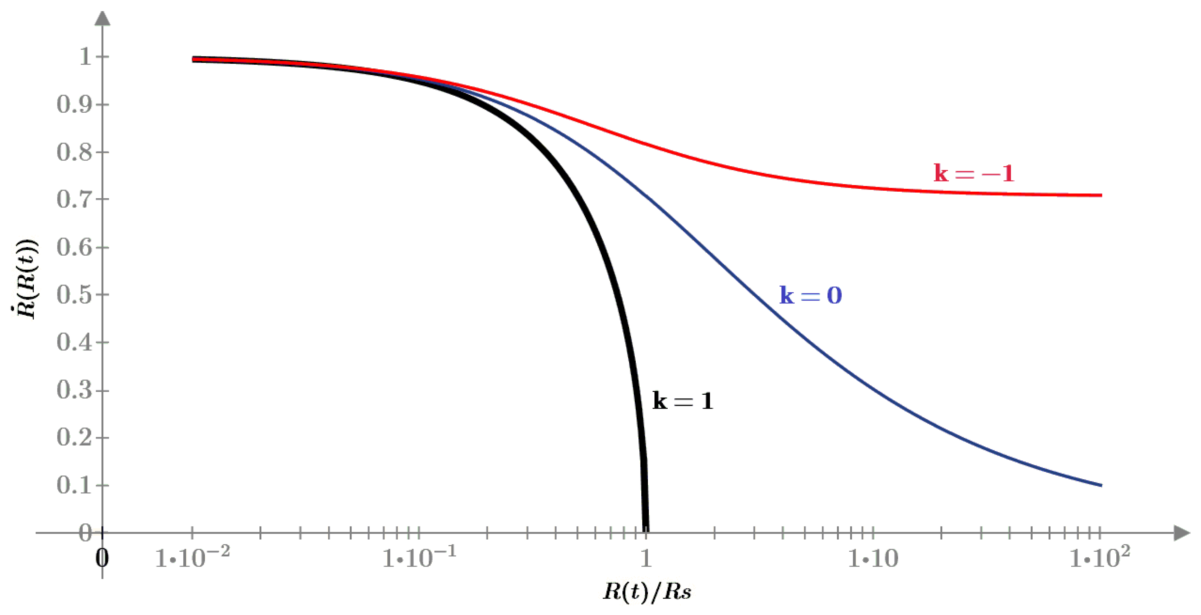
From the above expression we can now infer how the universe behaves for each type of curvature:

• Flat universe (k = 0): the universe expands indefinitely, with its expansion velocity gradually decreasing but never vanishing ($\dot{R}(ct)$→ 0 as R(ct) →∞).

• Open universe (k = −1): the universe also expands indefinitely, with the velocity tending asymptotically to $c/\sqrt{2}$ as R(ct) →∞.
• Closed universe (k = 1): the universe expands in a decelerated manner until it reaches the maximum size R_S, after which a phase of accelerated contraction begins.

The following figure shows the expansion velocity as a function of the radius R(t), the k parameter and the values shown in Table 3.

Figure 1. The rate of expansion of the universe as a function of its radius R(t) and the k value.

Figure 1. The rate of expansion of the universe as a function of its radius R(t) and the k value.

Differentiating with respect to time yields the acceleration of the cosmic expansion:

$$\ddot{R}(ct)={\displaystyle \frac{d\dot{R}(ct)}{cdt}}={\displaystyle \frac{d\dot{R}(ct)}{dR}}{\displaystyle \frac{dR}{cdt}}={\displaystyle \frac{d\dot{R}(ct)}{dR}}\dot{R}(ct)==-{\displaystyle \frac{1}{2}}{\displaystyle \frac{R_{S}R(ct)(R(ct)+2R_R)}{[(1-k)R^2(ct)+R_S(R(ct)+R_R){]}^2}}$$

(52)

where the negative sign indicates that the expansion is decelerated. Thus, the universe begins at R(0) = 0 with an initial expansion velocity equal to c, which gradually decreases over time, coming to rest only in the case of a closed universe (k = 1 ).

Substituting Eq. (50) into the metric (16), we obtain:

$$d{s}^2={\displaystyle \frac{R^2(ct)}{(1-k)R^2(ct)+R_s(R_R+R(ct))}}{c}^{2}d{t}^2-R^2(ct)({\displaystyle \frac{d{r}^2}{1-r^2}}+r^{2}d{\theta }^2+r^{2}si{n}^2\theta d{\mathsf{\varphi }}^2)$$

(53)

Introducing the variable change

$$d\tau =\sqrt{{\displaystyle \frac{R^2(ct)}{(1-k)R^2(ct)+R_s(R_R+R(ct))}}}\cdot dt$$

(54)

we recover the standard FLRW metric (where the scale factor a(τ) is replaced by the radius R(τ):

$$d{s}^2=c^{2}d{\tau }^2-R^2(\tau )({\displaystyle \frac{d{r}^2}{1-r^2}}+r^{2}d{\theta }^2+r^{2}si{n}^2\theta d{\varphi }^2)$$

(55)

Here, τ represents the proper time of a comoving observer, while t is the cosmic coordinate time.

To relate R with the coordinate time t, one needs to integrate

$$t={\displaystyle \frac{1}{c}}{\int }_0^R{\displaystyle \frac{dR}{\dot{R}}}$$

(56)

For Eq. (51), this integral has no known analytical solution. However, assuming a matter-dominated universe and using the approximation R(t) >> R_R, and for the closed universe, k = 1, we obtain

$$t(R)\simeq {\displaystyle \frac{1}{c}}{\int }_0^R\sqrt{{\displaystyle \frac{R_S}{R_S-R}}}dR={\displaystyle \frac{2R_S}{c}}(1-\sqrt{{\displaystyle \frac{R_S-R}{R_S}}})$$

(57)

4. Dynamics of the Universe According to a Comoving Observer

From the metric obtained in the previous section, the standard Friedmann equations can now be applied, which in our framework take the form:

$$H^2(\tau )={\displaystyle \frac{8\pi G}{3}}\rho (\tau )-{\displaystyle \frac{k{c}^2}{R^2(\tau )}}$$

(58)

$${\displaystyle \frac{\ddot{R}(\tau )}{R(\tau )}}=-{\displaystyle \frac{4\pi G}{3}}(\rho (\tau )+3p(\tau ))$$

(59)

Here, the Hubble parameter H(τ) is defined as

$$H(\tau )={\displaystyle \frac{\dot{R}(\tau )}{R(\tau )}}$$

(60)

From this point onward, we work in the comoving frame, where proper time τ is used instead of the coordinate time t. Accordingly, derivatives with respect to τ are denoted by $\dot{R}$ and $\ddot{R}$.

It is useful to introduce the concept of the critical density, defined as the density for which the universe would be spatially flat (k = 0):

$${\rho }_c(\tau )={\displaystyle \frac{3H(\tau {)}^2}{8\pi G}}$$

(61)

Dividing the second Friedmann equation by H²(τ), one obtains:

$$1={\displaystyle \frac{8\pi G}{3H^2(\tau )}}\rho (\tau )-{\displaystyle \frac{k{c}^2}{R^2(\tau )H^2(\tau )}}={\displaystyle \frac{\rho (\tau )}{{\rho }_c(\tau )}}-{\displaystyle \frac{k{c}^2}{R^2(\tau )H^2(\tau )}}$$

(62)

This can be expressed as

$$1=\Omega (\tau )+{\Omega }_k(\tau )$$

(63)

where we define the density parameter as

$$\Omega (\tau ):={\displaystyle \frac{\rho (\tau )}{{\rho }_c(\tau )}}$$

(64)

and the curvature parameter as

$${\Omega }_k(\tau ):=-{\displaystyle \frac{c^2}{R^2(\tau )H^2(\tau )}}$$

(65)

From these definitions, if ρ(τ) = ρ_c(τ), then Ω(τ) = 1 and consequently Ω_k(τ) = 0, implying a flat universe.

Repeating the same procedure as in the previous section, and using the same assumptions for matter and radiation densities together with the definitions of R_R and R_M given in Eq. (43), the first Friedmann equation yields:

$$\dot{R^2}(\tau )=c^2({\displaystyle \frac{R_S{R}_R}{R^2(\tau )}}+{\displaystyle \frac{R_M}{R(\tau )}}-k)=c^2({\displaystyle \frac{R_S{R}_R+R_{M}R(\tau )}{R^2(\tau )}}-k)$$

(66)

Previously, the radiation density was scaled with R_S, under the assumption that this would be the maximum radius attained by the expanding closed universe. Therefore, when R(τ) = R_S, the expansion must stop, i.e.

$$\dot{R^2}(t)=0\Rightarrow {\displaystyle \frac{R_S{R}_R+R_M{R}_S}{R_S^2}}=1$$

(67)

From which it follows that the maximum radius is

$$R_S=R_R+R_M$$

(68)

Considering the present-day matter density ρ_M ≈ ρ_c ≈ 9.31 x 10^-27 kg/m³ and the radiation density ρ_R ≈ 7.8 x 10^-31 kg/m³ we may approximate

$$R_S\simeq R_M={\displaystyle \frac{2G{M}_U}{c^2}}$$

(69)

Thus, we finally obtain

$$\dot{R}(\tau )\simeq c\sqrt{{\displaystyle \frac{R_S(R_R+R(\tau ))}{R^2(\tau )}}-k}$$

(70)

from which it follows that the transition from the radiation era to the matter era occurs when R(τ) ≥ R_R.

The following figure shows the expansion velocity as a function of the radius R(t), the k parameter and the values shown in Table 3.

The consequences that can be drawn from expression (70) and shown in the previous figure, are that the dynamics of the three universes are very similar for values R << R_S.

Figure 1. The rate of expansion of the universe as a function of its radius R(τ) and the k value.

Figure 1. The rate of expansion of the universe as a function of its radius R(τ) and the k value.

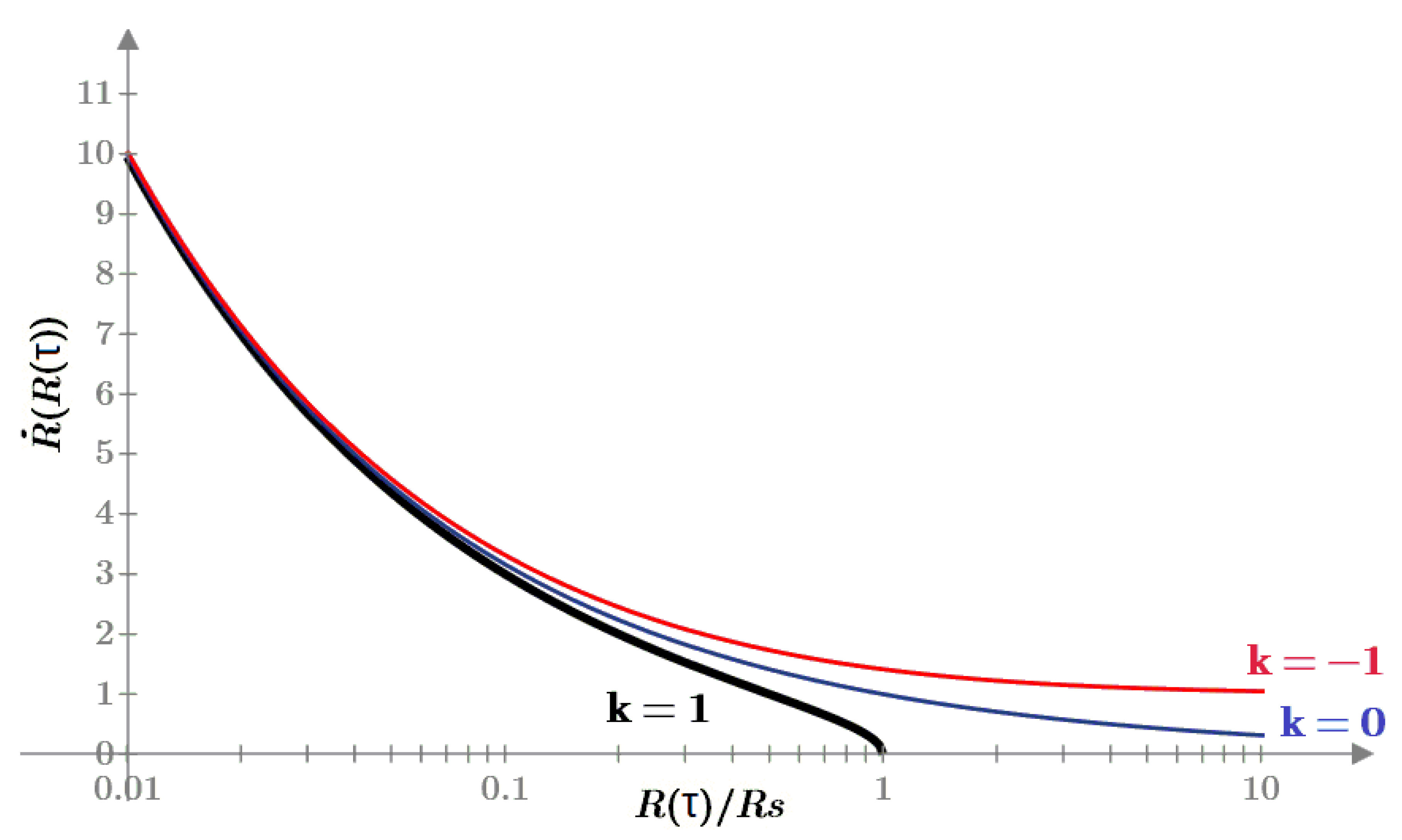
On the other hand, we can conclude that, similar to what was obtained for a coordinate observer, we have:

• Flat universe (k = 0): the universe will expand indefinitely, with the expansion velocity gradually decreasing but never reaching zero ($\dot{R}(ct)$→ 0 as R(ct) →∞)
• Open universe (k = −1): the universe will also expand indefinitely, with the expansion velocity gradually decreasing and tending to c when R(ct) →∞.
• Closed universe (k = 1): the universe will expand in a decelerated way until it reaches a maximum size R_S, at which point a phase of accelerated contraction of its radius will begin.

From Eq. (70), the Hubble parameter is computed as

$$H(\tau )=c{\displaystyle \frac{\sqrt{R_S(R_R+R(\tau ))-k{R}^2}}{R^2(\tau )}}$$

(71)

and the curvature parameter as

$${\mathsf{\Omega }}_k(\tau )={\displaystyle \frac{-R^2(\tau )}{R_S(R_R+R(\tau ))-k{R}^2(\tau )}}$$

(72)

Finally, differentiating Eq. (70), the cosmic acceleration is obtained as

$$\ddot{R}(\tau )=-{\displaystyle \frac{R_S(R(\tau )+2R_R)}{2R^3(\tau )}}{c}^2$$

(73)

value that is independent of k and which, using the definition of R_S given in Eq. (30), becomes

$$\ddot{R}(\tau )=-{\displaystyle \frac{G{M}_U}{R^2(\tau )}}(1+2{\displaystyle \frac{R_R}{R(\tau )}})$$

(74)

Therefore, we conclude that the expansion of the universe is decelerated, consistent with the result previously obtained.

4.1. Kinematic Framework and the Scope of Special Relativity

A noteworthy consequence of the dynamics derived for the comoving observer is that the expansion velocity of the hypersphere, Ṙ(τ), can formally exceed the speed of light c. Using the parameters from Table 3, its present-day value is calculated from (70) to be approximately 213c (independent of k).

This superluminal result does not signal a departure from General Relativity, but arises naturally from applying it to our proposed 5D metric. The apparent paradox is resolved by distinguishing between the comoving observer’s proper time τ and the coordinate observer’s time t. The expansion rate in the privileged frame, Ṙ(t), remains strictly subluminal, thus preserving causality. The superluminal value of Ṙ(τ) is a direct consequence of the time dilation experienced by comoving observers due to their extrinsic motion.

More broadly, our model's kinematic framework necessitates a re-evaluation of the scope of Special Relativity (SR) in a cosmological context. Two arguments underpin this view:

• The Existence of a Privileged Frame: The rest frame of the 5D bulk constitutes a privileged reference frame. While not directly accessible from within the 3-brane, its existence is incompatible with the global validity of the Principle of Relativity. Furthermore, for a closed universe, a comoving observer could, in principle, measure their absolute peculiar velocity and establish an absolute synchronization scheme, as shown in [16], leading to the "Generic Transformations" also derived therein.
• Cosmic Expansion: Independently of curvature, the expansion of space prevents the strict application of the Einstein synchronization convention, which requires fixed distances between clocks. The operational basis of SR is therefore fundamentally limited on cosmological scales.

Despite these fundamental limitations, SR emerges as an effective and highly accurate local working framework. Because absolute synchronization is not operationally accessible, the Einstein convention remains the only practical procedure, which by construction imposes the Lorentz transformations onto our measurements. In this sense, SR should be regarded not as a fundamental law of the universe, but as an emergent local symmetry—an excellent approximation for laboratory and most astrophysical contexts, but not the ultimate foundation of cosmology.

4.2. Radiation-Dominated Era

At this stage, we must distinguish between the two main evolutionary eras of the universe. For the radiation-dominated era, we have R(τ) << R_R. Since R_SR_R >> k R(τ), the first term inside the square root dominates over unity. Therefore, we obtain:

$$\dot{R}(\tau )\simeq {\displaystyle \frac{\sqrt{R_S{R}_R}}{R(\tau )}}\cdot c$$

(75)

This result shows that, during the radiation era, the universe expands as if it were completely flat, since the unity term inside the square root—which corresponds to the curvature contribution k—is negligible compared to the first term.

From Eq. (75), the Hubble parameter can be expressed as:

$$H_R(\tau )=c{\displaystyle \frac{\sqrt{R_S{R}_R}}{R^2(\tau )}}$$

(76)

and the curvature parameter as:

$${\Omega }_{kR}(\tau )=-{\displaystyle \frac{R^2(\tau )}{R_S{R}_R}}$$

(77)

Furthermore, integrating the expansion velocity in the radiation era yields:

$$R(\tau )=\sqrt{2c\tau \sqrt{R_R{R}_S}}$$

(78)

In this regime, the Hubble parameter becomes:

$$H_R(\tau )={\displaystyle \frac{\dot{R}(\tau )}{R(\tau )}}\simeq c{\displaystyle \frac{\sqrt{R_S{R}_R}}{R^2(\tau )}}={\displaystyle \frac{1}{2\tau }}$$

(79)

This implies that the Hubble parameter in a radiation-dominated universe depends only on cosmic time τ, and not on the initial density, as expected for a flat expanding universe.

Using the expression for R(τ), we can also compute the curvature parameter as:

$${\Omega }_{k_R}(\tau )=-{\displaystyle \frac{2c\tau }{\sqrt{R_S{R}_R}}}$$

(80)

Finally, differentiating Eq. (75), the acceleration of the expansion takes the form:

$$\ddot{R}(\tau )=-{\displaystyle \frac{2G{M}_U{R}_R}{R^3(\tau )}}=-{\displaystyle \frac{4G^2{M}_U{M}_R}{R^3(\tau )c^2}}$$

(81)

4.3. Matter-Dominated Era

For the matter-dominated era, we have R(t) >> R_R. In this regime, the expansion velocity becomes

$$\dot{R}(\tau )\simeq c\sqrt{{\displaystyle \frac{R_S}{R(\tau )}}-k}$$

(82)

From Eq. (82), if R(t) << R_S, the universe still expands as if it were spatially flat. In this limit, the curvature parameter can be approximated as

$${\Omega }_{k_M}(\tau )\simeq -{\displaystyle \frac{R(\tau )}{R_S}}$$

(83)

Thus, the curvature parameter directly measures the ratio between the current size of the universe and its maximum possible size R_S.

Integrating the expansion velocity leads to

$$R(\tau )=({\displaystyle \frac{3}{2}}c\tau \sqrt{R_S}{)}^{{\displaystyle \frac{2}{3}}}$$

(84)

In this case, the Hubble parameter becomes

$$H_M(\tau )={\displaystyle \frac{\dot{R}(\tau )}{R(\tau )}}\simeq c\sqrt{{\displaystyle \frac{R_S}{R^3(\tau )}}}={\displaystyle \frac{2}{3\tau }}$$

(85)

This result again coincides with that of a flat universe dominated by dust-like matter.

Finally, the acceleration of the expansion is obtained as

$$\ddot{R}(\tau )\simeq -{\displaystyle \frac{G{M}_U}{R^2(\tau )}}$$

(86)

5. Alternative to Dark Energy: A Luminosity–Redshift Bias in Type Ia Supernova

In the previous sections, we have shown that the universe described by our model—closed and evolving on the surface of a three-sphere—undergoes expansion, but in a decelerated manner. This result stands in direct contradiction with the standard ΛCDM paradigm, according to which the universe is currently undergoing accelerated expansion driven by a dark energy component.

In addition to this discrepancy, the proposed model faces a second apparent difficulty: its predicted age is too young to accommodate the oldest stellar objects observed to date, such as the so-called Methuselah star (HD 140283), whose estimated age exceeds 12 Gyr.

As an approximation, for a matter-dominated universe the present cosmic age τ0\tau_0τ0​ can be computed from Eq. (85) as

$${\tau }_0={\displaystyle \frac{2}{3H_0}}$$

(87)

Substituting the actual value H₀ = 73.0 km/s/Mpc, one obtains

$${\tau }_0\simeq 8.94\cdot 10^{9}years$$

(88)

which is clearly incompatible with the existence of the oldest known stellar populations. In order to recover an age close to the commonly accepted value of ∼13.8×10⁹ years, a significantly lower Hubble parameter, H0 ≃ 47 - 49 km/ s/ Mpc, would be required.

Although they may appear unrelated, these two issues—the accelerated expansion and the age problem—are in fact closely connected. The value of H₀ is inferred from distance–redshift relations, so any systematic bias in those relations directly propagates into the inferred expansion rate and, consequently, into the estimated age of the universe.

The hypothesis of accelerated expansion was originally proposed as a response to observations of Type Ia supernovae, which appeared systematically dimmer at high redshift than expected in a purely matter-dominated universe. In the standard interpretation, this dimming implies that distant supernovae are farther away than predicted by CDM cosmology, leading to the inference of an accelerated expansion phase.

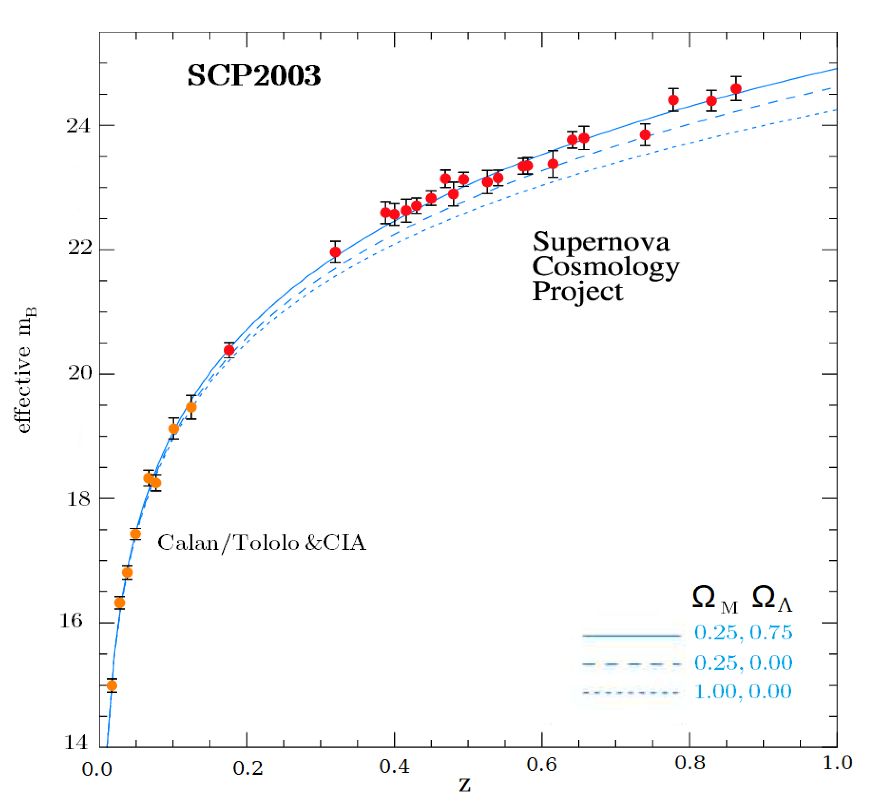
The figure below shows the Hubble diagram obtained by the Supernova Cosmology Project in 2003 1, which reports the effective value of m_B as a function of redshift z. We assume m_B is defined as:

$$m_B^{effective}=M+5\cdot \log \left(D_L\left(z,{\mathsf{\Omega }}_M,{\mathsf{\Omega }}_{\mathsf{\Lambda }}\right)\right)+25$$

(89)

where, in a ΛCDM universe with density parameters Ω_M and Ω_Λ, the luminosity distance is given by

$$D_L(z,{\mathsf{\Omega }}_M,{\mathsf{\Omega }}_{\mathsf{\Lambda }}))=(1+z)\cdot D_C(z,{\mathsf{\Omega }}_M,{\mathsf{\Omega }}_{\mathsf{\Lambda }})$$

(90)

And the comoving distance is

$$D_C(z,{\mathsf{\Omega }}_M,{\mathsf{\Omega }}_{\mathsf{\Lambda }})={\displaystyle \frac{c}{H_0}}{\int }_0^z{\displaystyle \frac{dz’}{\sqrt{{\mathsf{\Omega }}_M(1+z’{)}^3+{\mathsf{\Omega }}_{\mathsf{\Lambda }}}}}$$

(91)

Hence, the luminosity distance reads

$$D_L(z,{\mathsf{\Omega }}_M,{\mathsf{\Omega }}_{\mathsf{\Lambda }})={\displaystyle \frac{(1+z)\cdot c}{H_0}}{\int }_0^z{\displaystyle \frac{dz\text{'}}{\sqrt{{\mathsf{\Omega }}_M(1+z\text{'}{)}^3+{\mathsf{\Omega }}_{\mathsf{\Lambda }}}}}$$

(92)

For a CDM universe without dark energy (Ω_M = 1 and Ω_Λ = 0), this expression reduces to

$$D_L(z)={\displaystyle \frac{2c}{H_0}}(1+z)(1-{\displaystyle \frac{1}{\sqrt{1+z}}})$$

(93)

Figure 3. Hubble diagram obtained by the Supernova Cosmology Project in 2003.

Figure 3. Hubble diagram obtained by the Supernova Cosmology Project in 2003.

Recently, several studies 23 have suggested that the apparent need for dark energy may be an artefact arising from an unaccounted evolution of Type Ia supernova luminosity with cosmic time. In particular, younger progenitor systems (corresponding to higher redshifts) may intrinsically produce fainter explosions.

Although Type Ia supernovae are standardizable candles, their intrinsic luminosity is expected to evolve mildly with redshift due to well-known astrophysical effects such as progenitor metallicity, stellar population age, and the evolving mixture of progenitor channels.

Following this line of reasoning, we propose in this work the hypothesis that the intrinsic luminosity of Type Ia supernovae follows the relation

$$L(z)={\displaystyle \frac{L_0}{1+z}}$$

(94)

This correction does not arise from the geometry of the present model, but it removes the need for dark energy and, as shown below, leads to a self-consistent description of the full set of cosmological observables.

The observed flux is defined as

$$F(z)={\displaystyle \frac{L(z)}{4\pi D_L^2(z)}}$$

(95)

Taking into account the cosmological redshift factor (1+z) and the corresponding time-dilation between emission and observation, also given by(1+z), the observed flux scales as

$$F(z)\propto {\displaystyle \frac{L(z)}{(1+z{)}^2}}\propto {\displaystyle \frac{1}{(1+z{)}^3}}$$

(96)

Solving Eq. (95) for the luminosity distance, the standard expression

$$D_L\left(z\right)=r{R}_o\left(1+z\right)$$

(97)

Is replaced by

$$D_{Ld}\left(z\right)=r{R}_o{\left(1+z\right)}^{{\displaystyle \frac{3}{2}}}=D_L\left(z\right)\sqrt{1+z}$$

(98)

Therefore, the corrected luminosity distance becomes

$$D_{Ld}(z)={\displaystyle \frac{2c}{H_0}}(1+z{)}^{3/2}(1-{\displaystyle \frac{1}{\sqrt{1+z}}})={\displaystyle \frac{2c}{H_0}}(1+z)(\sqrt{1+z}-1)$$

(99)

Comparing this result with Eq. (90), we define an effective comoving distance

$$D_C^{eff}(z)={\displaystyle \frac{2c}{H_0}}(\sqrt{1+z}-1)$$

(100)

Including the luminosity evolution hypothesis L(z), one obtains

$$m_{Bd}^{eff}\left(z\right)=M+5\cdot \log \left(D_{Ld}\left(z\right)\right)+25=M+5\cdot \log \left(D_L\left(z\right)\sqrt{1+z}\right)+25$$

(101)

and if we continue to operate, we get that:

$$m_{Bd}^{eff}\left(z\right)=M+5\cdot \log \left(D_L\left(z\right)\right)+{\displaystyle \frac{5}{2}}\cdot \log \left(1+z\right)+25$$

(102)

Therefore, the effective value of m_Bd^eff(z) will be:

$$m_{Bd}^{eff}\left(z\right)=m_B^{eff}\left(z\right)+{\displaystyle \frac{5}{2}}\cdot \log \left(1+z\right)=m_B^{eff}\left(z\right)+\mathsf{\Delta }{m}_B(z)$$

(103)

As a result, introducing the luminosity decay (94) leads to a magnitude correction

$$\mathsf{\Delta }{m}_B(z)={\displaystyle \frac{5}{2}}\log (1+z)$$

(104)

If we now represent graphically (red line) the previous expression taking as m_B^eff(z) the theoretical values for a universe composed only of cold matter (i.e. Ω_M = 1.0 and Ω_Λ = 0.0) and superimpose it on the Hubble diagram obtained by the Supernova Cosmology Project, we will see that the values of m_Bd^eff(z) obtained with the expression (103) coincides perfectly with those obtained for a universe with dark matter and dark energy with densities Ω_M = 0.25 and Ω_Λ = 0.75 respectively.

Figure 4. In red, the m_Bd^eff(z) values superimposed on the Hubble diagram of the Supernova Cosmology Project.

Figure 4. In red, the m_Bd^eff(z) values superimposed on the Hubble diagram of the Supernova Cosmology Project.

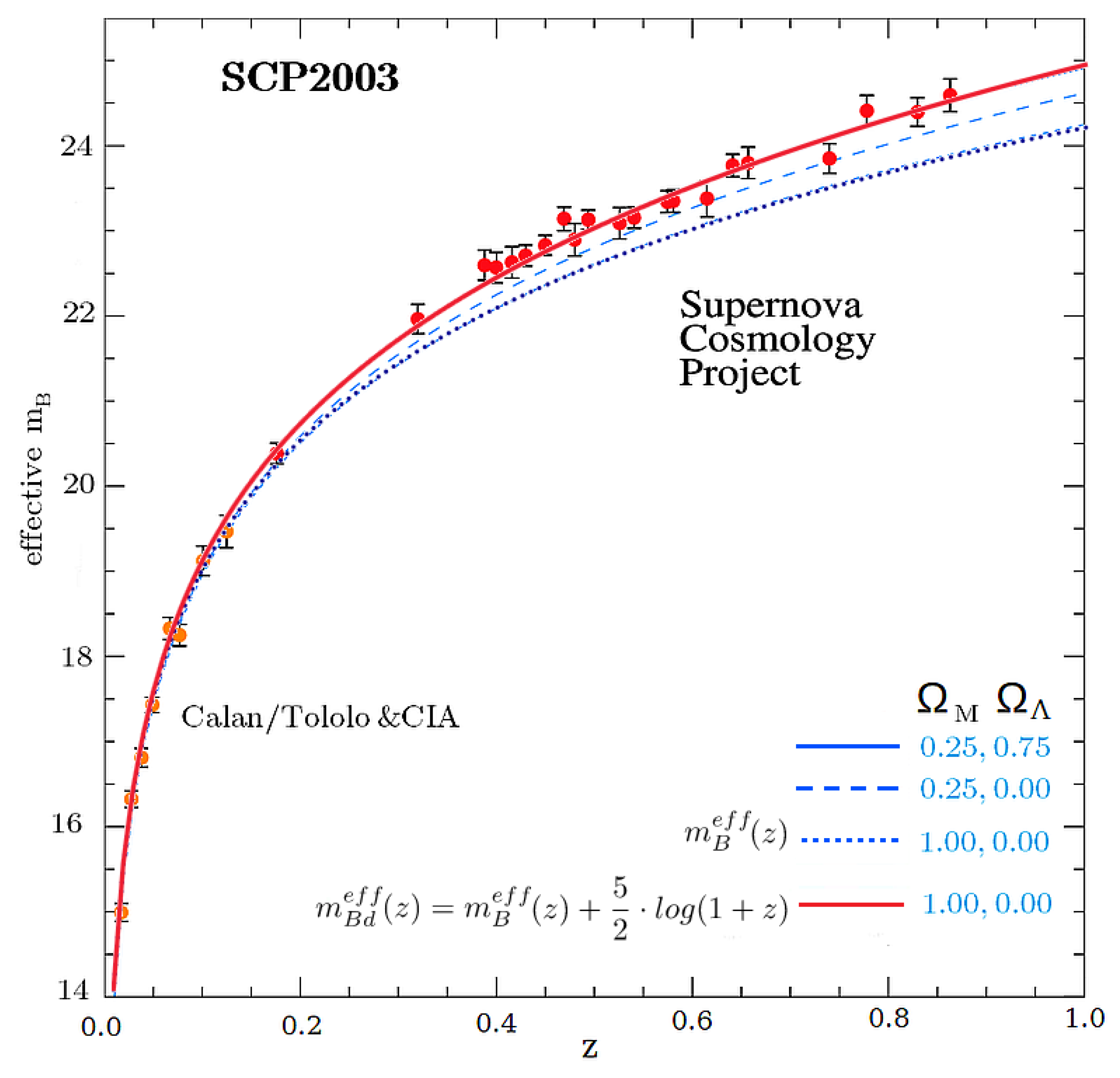
Therefore, the apparent dimming of distant Type Ia supernovae—commonly interpreted as evidence for accelerated expansion—can instead be understood as a luminosity–redshift bias. This removes the need to postulate a dark energy component.

This result supports the conclusion that the universe is in fact undergoing decelerated expansion, fully consistent with the theoretical predictions of the five-dimensional cosmological model presented here.

The following table lists the numerical values obtained from the above expressions. In order to match the observational data in Fig. 4, an absolute magnitude M=−19.2 has been adopted.

Table 1. Values of m_Bd^eff(z) for different models.

z	mBeff(z)ΛCDM	mBeff(z)CDM	ΔmB(z)	mBdeff(z)	mBdeff(z) - mBeff(z)ΛCDM
0.1	19.03	18.92	0.10	19.02	-0.010
0.2	20.68	20.47	0.20	20.67	-0.014
0.3	21.69	21.39	0.28	21.68	-0.013
0.4	22.42	22.05	0.37	22.42	-0.007
0.5	23.01	22.57	0.44	23.01	0.003
0.6	23.49	23.00	0.51	23.51	0.016
0.7	23.91	23.36	0.58	23.94	0.031
0.8	24.27	23.68	0.64	24.32	0.048
0.9	24.59	23.96	0.70	24.66	0.067
1.0	24.88	24.21	0.75	24.96	0.087

Table 1. Values of m_Bd^eff(z) for different models.

z	mBeff(z)ΛCDM	mBeff(z)CDM	ΔmB(z)	mBdeff(z)	mBdeff(z) - mBeff(z)ΛCDM
0.1	19.03	18.92	0.10	19.02	-0.010
0.2	20.68	20.47	0.20	20.67	-0.014
0.3	21.69	21.39	0.28	21.68	-0.013
0.4	22.42	22.05	0.37	22.42	-0.007
0.5	23.01	22.57	0.44	23.01	0.003
0.6	23.49	23.00	0.51	23.51	0.016
0.7	23.91	23.36	0.58	23.94	0.031
0.8	24.27	23.68	0.64	24.32	0.048
0.9	24.59	23.96	0.70	24.66	0.067
1.0	24.88	24.21	0.75	24.96	0.087

5.1. Resolution of the Hubble Tension: The Hubble Law at low redshift (z << 1)

One of the most pressing enigmas in modern cosmology is the so-called 'Hubble Tension,' a statistically significant discrepancy (~ 5σ) between the expansion rate derived from the early universe (CMB) and direct local measurements. While Planck data, interpreted within the ΛCDM framework, favors a value of H₀ ≈ 67.4 km/s/Mpc, the local distance ladder based on Cepheids and Type Ia Supernovae yields a notably higher value of H₀ ≈ 73 km/s/Mpc. This persistent conflict suggests either an overlooked systematic error in astrophysical calibrations or, more profoundly, the existence of 'New Physics' beyond the standard cosmological model.

As discussed in the previous section, our five-dimensional cosmological model proposes that the intrinsic luminosity of Type Ia supernovae decreases with redshift according to L(z)∝(1+z)^-1.

This luminosity evolution leads to the modified luminosity distance defined in Eq. (98), which can be written as

$$D_{Ld}\left(z\right)=r{R}_o{\left(1+z_{eff}\right)}^{{\displaystyle \frac{3}{2}}}=r{R}_o(1+\mathrm{z})$$

(105)

From this identification, one obtains the relation

$$1+\mathrm{z}=(1+z_{eff}{)}^{3/2}$$

(106)

It is important to emphasize that the above expression is purely a mathematical reparametrization and carries no physical meaning. In particular, it does not imply the existence of any additional redshift affecting photon propagation. The parameter z_eff is introduced solely as a bookkeeping device that accounts for the systematic overestimation of luminosity distances when the redshift dependence of SN Ia luminosity is neglected.

Using this reparametrization, the corrected luminosity distance for a CDM universe can be written as

$$D_{Ld}^{eff}(z)={\displaystyle \frac{2c}{H_0}}(1+z)D_C^{eff}(z_{eff})$$

(107)

Substituting Eq. (100) into the above expression yields

$$D_{Ld}^{eff}(z)={\displaystyle \frac{2c}{H_0}}(1+z)(\sqrt{1+z_{eff}}-1)$$

(108)

Ussing Eq. (106) to eliminate z_eff , one finally obtains

$$D_{Ld}^{eff}(z)={\displaystyle \frac{2c}{H_0}}(1+z)(\sqrt[3]{1+z}-1)$$

(109)

By contrast, for a ΛCDM universe we retain the standard expression given in Eq. (92), using the observationally inferred value H₀^obs≃73 km/ s/Mpc.

Since both expressions must describe the same observed luminosity distance, consistency requires

$${\displaystyle \frac{2c}{H_0}}(1+z)(\sqrt[3]{1+z}-1)={\displaystyle \frac{2c}{H_0^{obs}}}(1+z)(\sqrt[2]{1+z}-1)$$

(110)

Solving for H₀, we obtain

$$H_0=H_0^{obs}{\displaystyle \frac{\sqrt[3]{1+z}-1}{\sqrt[2]{1+z}-1}}$$

(111)

Using the first-order Taylor expansion

$$(1+x{)}^n\simeq 1+nx$$

(112)

we obtain, for z << 1:

$$H_0\simeq H_0^{obs}{\displaystyle \frac{1+\frac{1}{3}z-1}{1+\frac{1}{2}z-1}}={\displaystyle \frac{2}{3}}{H}_0^{obs}$$

(113)

Therefore, in the local universe, the Hubble constant inferred from Type Ia supernova observations is systematically overestimated if the luminosity evolution of SNe Ia is ignored. Adopting the SH0ES value H₀^obs ≈ 73 km/s/Mpc, the true Hubble parameter in our model is

$${\mathit{H}}_0\simeq {\displaystyle \frac{H_0^{obs}}{1.5}}={\displaystyle \frac{73km/s/Mpc}{1.5}}=48.7\mathit{k}\mathit{m}/\mathit{s}/\mathit{M}\mathit{p}\mathit{c}$$

(114)

From this point onward, the present value of the Hubble parameter H₀ will be taken to be the one given above, while H₀^obs denotes the value inferred from standard supernova-based analyses.

It is important to note that this result does not resolve the Hubble tension by converging toward the Planck value. Instead, it suggests that the true physical expansion rate of the universe is significantly lower than both CMB- and distance-ladder-based estimates. This is consistent with the spirit of the present work: since the Planck value of H₀ is model-dependent—derived under the assumption of a flat ΛCDM cosmology—there is no reason for an alternative geometric framework to reproduce it.

In this interpretation, the Hubble tension arises because standard analyses interpret the redshift-dependent dimming of Type Ia supernovae as an increase in luminosity distance, thereby contaminating the inferred value of the Hubble constant.

5.2. The Age of the Universe

Assuming a matter-dominated universe—as will be dynamically justified in later sections—we can use (87) to obtain the standard relation for the age of the universe τ₀ in terms of the real Hubble parameter. Substituting the corrected value H₀ = 48.7 km/s/Mpc derived in the previous section, we obtain

$${\mathit{\tau }}_0\simeq 13.4\cdot 10^9\mathit{y}\mathit{e}\mathit{a}\mathit{r}\mathit{s}$$

(115)

This value is in excellent agreement with the age of the universe inferred from Planck 2018 data within the ΛCDM framework, τ₀≃13.787×10⁹ years, despite being derived here under fundamentally different assumptions.

Most importantly, this result resolves the severe timescale problem that would otherwise arise in a matter-dominated cosmology when using the locally inferred value H₀^obs≃73 km/ s/ Mpc/, which would imply an unacceptably young universe (τ₀ ∼9 Gyr). In the present framework, the reduced value of H0 emerges naturally as a consequence of correcting the luminosity–redshift relation of Type Ia supernovae, and no additional dark energy component is required.

Therefore, the age of the universe provides an independent and non-trivial consistency check of the model: once the supernova luminosity bias is accounted for, a decelerated, matter-dominated expansion history becomes fully compatible with the observed ages of the oldest stellar populations.

5.3. Application to Supernova Hubble Diagrams

In the previous sections, we introduced the hypothesis that the intrinsic luminosity of Type Ia supernovae decreases with cosmological redshift according to L(z)∝(1+z)⁻¹. This assumption led to a modification of the inferred luminosity distance in supernova Hubble diagrams, which in turn affects both the inferred value of the Hubble parameter H₀ and the estimated age of the universe. These effects were parametrized through the introduction of an effective redshift z_effz and a distinction between the observed Hubble constant H₀^obs and the true physical value H₀.

It is now necessary to verify that, once these corrections are consistently applied, the supernova Hubble diagrams remain well fitted without invoking a dark energy component. To this end, we recompute the effective apparent magnitude m_B^eff(z) using the corrected expressions derived in the previous sections, adopting the revised value of the Hubble parameter and the effective redshift mapping.

Following table summarizes the comparison between the effective magnitudes obtained in a standard ΛCDM cosmology and those derived in the present framework for a matter-dominated universe with luminosity evolution.

Table 2. Values of m_Bd^eff(z) for different models.

z	mBdeff(z)ΛCDM	mBdeff(z)	mBdeff(z) - mBeff(z)ΛCDM
0.1	19.03	19.00	-0.027
0.2	20.68	20.63	-0.047
0.3	21.69	21.63	-0.061
0.4	22.42	22.36	-0.069
0.5	23.01	22.94	-0.073
0.6	23.49	23.42	-0.072
0.7	23.91	23.84	-0.068
0.8	24.27	24.20	-0.063
0.9	24.59	24.53	-0.054
1.0	24.88	24.83	-0.044

Table 2. Values of m_Bd^eff(z) for different models.

z	mBdeff(z)ΛCDM	mBdeff(z)	mBdeff(z) - mBeff(z)ΛCDM
0.1	19.03	19.00	-0.027
0.2	20.68	20.63	-0.047
0.3	21.69	21.63	-0.061
0.4	22.42	22.36	-0.069
0.5	23.01	22.94	-0.073
0.6	23.49	23.42	-0.072
0.7	23.91	23.84	-0.068
0.8	24.27	24.20	-0.063
0.9	24.59	24.53	-0.054
1.0	24.88	24.83	-0.044

From this comparison, we observe that the maximum deviation between both models is approximately −0.07 magnitudes over the entire redshift range considered. This level of agreement is well within the observational dispersion of current Type Ia supernova datasets and demonstrates that the proposed luminosity–redshift dependence is sufficient to reproduce the observed Hubble diagram without requiring an accelerated expansion phase.

Therefore, the apparent dimming of distant supernovae—traditionally interpreted as evidence for dark energy—can be fully accounted for by a mild, monotonic evolution of supernova luminosity with cosmic time. Within this framework, the universe undergoes a decelerated expansion consistent with matter domination, while simultaneously yielding a corrected Hubble constant and a cosmic age of approximately 13.4 Gyr, in close agreement with independent cosmological constraints.

6. Alternative to Inflation: The Link between CURVATURE and Homogeneity and Synchronicity

6.1. Cosmic Inflation: Motivation, Framework and Open Issues

The standard cosmological model, based on an FLRW metric that is observationally very close to flat and dominated at early times by radiation, faces three fundamental problems when extrapolated toward the past: the horizon problem, the flatness problem, and the overproduction of topological defects predicted by grand-unified theories.

To solve these problems the mechanism of cosmic inflation was proposed, first introduced by Guth 2 and later developed by Linde, Albrecht and Steinhardt. Inflation consists of a brief period of accelerated, quasi-exponential expansion of the early universe, of the form:

$$a(t)\propto e^{Ht},\hspace{1em}(H\simeq \mathrm{c}\mathrm{o}\mathrm{n}\mathrm{s}\mathrm{t}\mathrm{a}\mathrm{n}\mathrm{t}\mathrm{e})$$

(116)

lasting for a very short interval (roughly ∼10⁻³⁶ a 10⁻³² s after the Big Bang), driven by a scalar field (the inflaton) with an appropriate potential. During inflation the inflaton energy density behaves approximately as

$${\rho }_{\varphi }\simeq V(\varphi ),p_{\varphi }\simeq -V(\varphi )$$

(117)

so that the pressure is negative and the expansion accelerates. This process exponentially stretches any previously causal region, rendering the observable universe homogeneous and isotropic and strongly suppressing spatial curvature. It also dilutes relics (such as magnetic monopoles) outside our observable patch, and provides a natural mechanism to generate quantum primordial perturbations with an almost scale-invariant spectrum—in very good agreement with the cosmic microwave background observations and the large-scale structure.

Nevertheless, inflation raises its own open questions: the particle-physics origin of the inflaton, the specific shape and tuning of the inflaton potential, the need for appropriate initial conditions to start and stop inflation, and conceptual consequences such as eternal inflation and the associated measure/multiverse problems in some realizations. These limitations motivate the study of alternative scenarios capable of explaining homogeneity, flatness and the observed perturbation spectrum without invoking a dedicated inflationary phase.

6.2. New Hypothesis: The Relation Between Curvature and Homogeneity

The tree fundamental problems of the early universe (flatness, horizon and monopole problems) can be conceptually separated into two distinct categories: a problem of initial state and a problem of coherent evolution.

The flatness and monopole problems are primarily issues of the initial state. The flatness problem questions why the universe began with a density so extraordinarily close to the critical value. The monopole problem arises because, in a standard Big Bang, causally disconnected regions would undergo phase transitions independently, creating a vast number of topological defects. A universe that began in a state of extreme initial homogeneity, with minimal density fluctuations, would naturally alleviate both of these issues.

The horizon problem, on the other hand, is an issue of coherent evolution. It questions how causally disconnected regions, even if they started with similar initial conditions, managed to evolve in lockstep to reach the exact same temperature at the time of recombination. A standard, non-inflationary evolution within General Relativity does not provide a mechanism to maintain this coherence over cosmological distances.

Therefore, any complete alternative to inflation must provide separate solutions for both challenges: a physical principle that dictates a highly uniform initial state, and a kinematic framework that ensures its coherent evolution. This is the core of our proposal.

We first address the problem of coherent evolution through the kinematic framework of our 5D model, which, as discussed previously, establishes a global cosmic time. This absolute simultaneity ensures that all regions of the universe evolve synchronously, providing a natural solution to the horizon problem.

Then we address the problem of the initial state by postulating that cosmic curvature and inhomogeneity are intrinsically linked in such a way that a universe is spatially flat (k = 0) if and only if it is perfectly homogeneous. This law implies that a nearly flat universe, as we observe today, must have originated from a state of extraordinary homogeneity, thus resolving the flatness and monopole problems simultaneously.

To support this claim, let us employ the averaged Friedmann equations (see 6):

$$H^2={\displaystyle \frac{8\pi G}{3}}⟨\rho ⟩-{\displaystyle \frac{k{c}^2}{R^2}}+\mathcal{B}(⟨{\delta }_{\rho }^2⟩)$$

(118)

where $⟨{\delta }_{\rho }^2⟩$ is the mean density of the universe, and

$$⟨{\delta }_{\rho }^2⟩={\displaystyle \frac{⟨({\rho }_i-⟨\rho ⟩{)}^2⟩}{⟨\rho {⟩}^2}}={\displaystyle \frac{{\sigma }_{\rho }^2}{⟨\rho {⟩}^2}}$$

(119)

quantifies the relative variance of density fluctuations. The term $\mathcal{B}(⟨{\delta }_{\rho }^2⟩)$ represents the so-called backreaction, which encapsulates nonlinear effects of inhomogeneities. Such inhomogeneities are ultimately rooted in quantum fluctuations prior to the Planck era (since, by the uncertainty principle, spacetime at the Planck scale cannot be perfectly smooth but must exhibit intrinsic quantum fluctuations in both energy density and geometry/curvature).

Equation (118) can be rewritten as

$$H^2={\displaystyle \frac{8\pi G}{3}}(⟨\rho ⟩+{\displaystyle \frac{3}{8\pi G}}\mathcal{B}(⟨{\delta }_{\rho }^2⟩))-{\displaystyle \frac{k{c}^2}{R^2}}$$

(120)

From the previous expression it can be deduced that the $\mathcal{B}(⟨{\delta }_{\rho }^2⟩)$ term must have the dimensions of a density; therefore, we may propose that it takes the form

$$\rho =⟨\rho ⟩+n\cdot {\sigma }_{\rho }$$

(121)

with n an integer, then it follows that

$$\mathcal{B}(⟨{\delta }_{\rho }^2⟩)={\displaystyle \frac{8\pi G}{3}}n\cdot {\sigma }_{\rho }$$

(122)

Hence,

$$H^2={\displaystyle \frac{8\pi G}{3}}\rho -{\displaystyle \frac{k{c}^2}{R^2}}={\displaystyle \frac{8\pi G}{3}}(⟨\rho ⟩+n\cdot {\sigma }_{\rho })-{\displaystyle \frac{k{c}^2}{R^2}}$$

(123)

The averaged Friedmann equation thus becomes

$$H^2={\displaystyle \frac{8\pi G}{3}}⟨\rho ⟩(1+n\cdot {\displaystyle \frac{{\sigma }_{\rho }}{⟨\rho ⟩}})-{\displaystyle \frac{k{c}^2}{R^2}}={\displaystyle \frac{8\pi G}{3}}⟨\rho ⟩(1+n\cdot \sqrt{⟨{\delta }_{\rho }^2⟩})-{\displaystyle \frac{k{c}^2}{R^2}}$$

(124)

Dividing by H², we obtain

$$1={\displaystyle \frac{⟨\rho ⟩}{{\rho }_c}}(1+n\cdot \sqrt{⟨{\delta }_{\rho }^2⟩})-{\displaystyle \frac{k{c}^2}{R^2{H}^2}}$$

(125)

If we impose that all universes have mean density equal to the critical density,

$$⟨\rho ⟩={\rho }_c$$

(126)

then

$$1=(1+n\cdot \sqrt{⟨{\delta }_{\rho }^2⟩})+{\Omega }_k=\Omega +{\Omega }_k$$

(127)

This gives the effective density parameter as

$$\Omega =1+n\cdot \sqrt{⟨{\delta }_{\rho }^2⟩}$$

(128)

and the curvature parameter as

$${\Omega }_k=-n\cdot \sqrt{⟨{\delta }_{\rho }^2⟩}$$

(129)

At this stage, the choice of n is crucial. In this work, we adopt the value n = 1/2 in the expression (121). This choice is physically motivated by the quantum origin of primordial density fluctuations at the end of the Planck era. We postulate that their effective amplitude corresponds to the zero-point energy of the underlying quantum field, (1/2) ħω, justifying the factor n = 1/2 as the characteristic deviation associated with the linear regime of quantum vacuum fluctuations. Therefore, (121) becomes

$$\rho =⟨\rho ⟩+{\displaystyle \frac{1}{2}}\cdot {\sigma }_{\rho }$$

(130)

and we finally obtain

$${\mathsf{\Omega }}_k=-{\displaystyle \frac{1}{2}}\cdot \sqrt{⟨{\delta }_{\rho }^2⟩}$$

(131)

Thus, under these assumptions, we arrive at the intended conclusion: the universe is flat (k = 0) if and only if it is perfectly homogeneous (Ω_k = 0):

$$k=0⟺{\Omega }_k=0$$

(132)

Moreover, we have obtained that the curvature of the universe is proportional to its level of homogeneity: the more homogeneous the universe, the flatter its geometry, and vice versa. In this way, the flatness and monopole problems are simultaneously resolved under the single condition that the universe was sufficiently flat (homogeneous) at its origin.

Finally, it is important to note that, by defining the density ρ in (121) with the "+" sign, the resulting density is greater than the critical density, which necessarily implies k = 1, making the universe closed. Although this definition may seem arbitrary, it is adopted because the existence of structures requires overdensities (+ n σ_ρ), which implies ρ_eff > ρ_c, which in turn requires k = +1. Therefore, the existence of galaxies in our model predicts a closed universe.

In summary, our framework offers an alternative to inflation by addressing the problems of the early universe with two complementary principles. First, the flatness and initial homogeneity problems are resolved by the postulated law |Ω_k| = 1/2 δ_ρ, which intrinsically links the global geometry to the amplitude of density fluctuations, implying a near-flat and highly uniform initial state. Second, the horizon problem is addressed by the kinematic structure of our model. The existence of a globally defined cosmic time establishes a form of absolute simultaneity, ensuring that all regions of the hypersphere, having started from this uniform state, evolve synchronously. This coherent evolution, governed by a universal timeline, eliminates the need for a causal connection between distant regions to explain their identical temperatures at recombination.

6.3. Evolution of Density Fluctuations δ_ρ

In this section, we study how density fluctuations evolve with the cosmic expansion through equation (131).

For notational convenience, we first define the relative fluctutations, δV, for a physical variable V (density, temperature, mass...) as the root mean square (RMS) of its fluctuations,

$${\delta }_V:=\sqrt{<{\delta }_V^2>}={\displaystyle \frac{{\sigma }_V}{⟨V⟩}}={\displaystyle \frac{{\sigma }_V}{V}}$$

(133)

where σ_V are absolute standard deviations.

With this definition, our fundamental law (131) can be written in the more compact form:

$${\mathsf{\Omega }}_k=-{\displaystyle \frac{1}{2}}\cdot {\delta }_{\rho }$$

(134)

Similarly, for simplicity, we will omit the explicit dependence on the proper time τ in the following expressions, so that it is understood that e.g. R = R(τ) and Ω_k = Ω_k(τ).

From equation (65), we recall that

$${\Omega }_k(\tau ):=-{\displaystyle \frac{c^2}{R^2(\tau )H^2(\tau )}}=-{\displaystyle \frac{c^2}{{\dot{R}}^2(\tau )}}$$

(135)

Substituting the expansion velocity from (70) into the above expression, we obtain

$${\mathsf{\Omega }}_k(\tau )=-{\displaystyle \frac{1}{2}}\cdot {\delta }_{\rho }=-{\displaystyle \frac{R^2}{R_S(R_R+R)-R^2}}$$

(136)

which directly yields

$${\delta }_{\rho }={\displaystyle \frac{2R^2}{R_S(R_R+R)-R^2}}$$

(137)

If the total density is given by the sum of matter and radiation, and assuming that the total variance is the sum of the two variances, one finds

$${\delta }_{\rho }={\displaystyle \frac{{\sigma }_{{\rho }_M}+{\sigma }_{{\rho }_R}}{{\rho }_M+{\rho }_R}}={\displaystyle \frac{2R^2}{R_S(R_R+R)-R^2}}$$

(138)

which implies

$${\sigma }_{{\rho }_M}+{\sigma }_{{\rho }_R}={\displaystyle \frac{2R^2}{R_S(R_R+R)-R^2}}({\rho }_M+{\rho }_R)$$

(139)

Therefore,

$${\sigma }_{{\rho }_M}={\displaystyle \frac{2R^2}{R_S(R_R+R)-R^2}}\cdot {\rho }_M$$

(140)

$${\sigma }_{{\rho }_R}={\displaystyle \frac{2R^2}{R_S(R_R+R)-R^2}}\cdot {\rho }_R$$

(141)

Using the approximation R_M ≈ R_S together with the definitions of the densities in terms of the characteristic radii R_S and R_R,

$${\rho }_M={\displaystyle \frac{3c^2{R}_S}{8\pi G{R}^3}},{\rho }_R={\displaystyle \frac{3c^2{R}_R{R}_S}{8\pi G{R}^4}}$$

(142)

we obtain

$${\sigma }_{{\rho }_M}={\displaystyle \frac{R_S}{R_S(R_R+R)-R^2}}\cdot {\displaystyle \frac{3c^2}{4\pi GR}}$$

(143)

$${\sigma }_{{\rho }_R}={\displaystyle \frac{R_S}{R_S(R_R+R)-R^2}}\cdot {\displaystyle \frac{3c^2{R}_R}{4\pi G{R}^2}}$$

(144)

For |Ω_k| ≈ 0, i.e., R_S(R_R+R)>>R², these simplify to

$${\sigma }_{{\rho }_M}={\displaystyle \frac{3c^2}{4\pi GR(R_R+R)}}$$

(145)

$${\sigma }_{{\rho }_R}={\displaystyle \frac{3c^2{R}_R}{4\pi G{R}^2(R_R+R)}}$$

(146)

Adding both contributions, we obtain

$${\sigma }_{\rho }={\sigma }_{{\rho }_M}+{\sigma }_{{\rho }_R}={\displaystyle \frac{R_S}{R_S(R_R+R)-R^2}}\cdot {\displaystyle \frac{3c^2}{4\pi G}}\cdot {\displaystyle \frac{R+R_R}{R^2}}\simeq {\displaystyle \frac{3c^2}{4\pi G{R}^2}}$$

(147)

Dividing each variance (143) and (144) by its corresponding mean density, we find

$${\displaystyle \frac{{\sigma }_{{\rho }_M}}{{\rho }_M}}={\displaystyle \frac{2R^2}{R_S(R_R+R)-R^2}}={\displaystyle \frac{{\sigma }_{{\rho }_R}}{{\rho }_R}}$$

(148)

Thus, we obtain the key result

$${\delta }_{{\rho }_M}={\delta }_{{\rho }_R}$$

(149)

which implies that the universe exhibits pure adiabatic perturbations. This equality is not imposed a priori, as in the ΛCDM model where adiabaticity is required to match observations, but rather emerges here as a direct consequence of the geometric dynamics of the 3-sphere and of the condition |Ω_k| = 1/2 δ_ρ.

Physically, this means that no relative entropy perturbations exist between different components, and therefore all species fluctuate in phase with the same relative amplitude. The main consequences are: the coherence in the evolution of inhomogeneities across cosmic time, the conservation of the gravitational potential at superhorizon scales, and the compatibility with the observed adiabatic anisotropy pattern in the cosmic microwave background (CMB).

Finally, we note that the condition ${\delta }_{{\rho }_M}={\delta }_{{\rho }_R}$ directly implies

$$\left|{\mathsf{\Omega }}_k\right|={\displaystyle \frac{1}{2}}{\delta }_{\rho }={\displaystyle \frac{1}{2}}{\displaystyle \frac{{\sigma }_{{\rho }_M}+{\sigma }_{{\rho }_R}}{{\rho }_M+{\rho }_R}}\simeq {\displaystyle \frac{1}{2}}{\delta }_{{\rho }_M}$$

(150)

during the matter-dominated era, and

$$\left|{\mathsf{\Omega }}_k\right|={\displaystyle \frac{1}{2}}{\delta }_{\rho }\simeq {\displaystyle \frac{1}{2}}{\delta }_{{\rho }_R}$$

(151)

during the radiation-dominated era.

6.4. Evolution of Temperature Fluctuations δ_T

Using the fact that the temperature of the universe is related to the radiation density through

$$T({\rho }_R)={\displaystyle \frac{\sqrt[4]{{\rho }_R{\hslash }^3{c}^5}}{k_B}}=C\cdot {\rho }_R^{1/4}$$

(152)

where C is a proportionality constant. Differentiating this expression and dividing by the mean value of T, we immediately obtain

$${\delta }_T={\displaystyle \frac{1}{4}}{\delta }_{{\rho }_R}$$

(153)

In the case of a matter-dominated universe — corresponding to the present epoch — and making use of Eq. (150), we find

$${\delta }_T={\displaystyle \frac{1}{4}}{\delta }_{{\rho }_R}={\displaystyle \frac{1}{4}}{\delta }_{{\rho }_M}\simeq {\displaystyle \frac{1}{4}}{\delta }_{\rho }={\displaystyle \frac{1}{2}}\left|{\Omega }_K\right|$$

(154)

Equivalently,

$$\left|{\mathsf{\Omega }}_k\right|=2{\delta }_T=2\cdot \sqrt{⟨{\delta }_T^2⟩}$$

(155)

This result provides a direct link between the observed temperature anisotropies in the CMB and the global curvature of the universe, reinforcing the interpretation that adiabatic perturbations and spatial geometry are inherently coupled in this framework.

6.5. Application and Results: The CMB

At this stage, it is natural to test whether the framework can yield quantitative predictions starting from the observed properties of the Cosmic Microwave Background (CMB). We use the present-day mean temperature T_CMB = 2.7255 K and the amplitude of its anisotropies δ_TCMB = 1.1x10^-5 57.

From the relation previously derived between curvature and homogeneity, the statistical properties of the CMB should provide direct information about the current curvature parameter of the universe. Under this assumption, we obtain

$$\left|{\Omega }_{k0}\right|=2\cdot \sqrt{⟨{\delta }_{T_{CMB}}^2⟩}\simeq 2.2\cdot 10^{-5}$$

(156)

In addition to the CMB values, we adopt H₀ = 48.7 km/s/Mpc. Using the equations developed above, we can then compute the present radius of the hypersphere, the total mass of the universe, the radiation density, and the cosmic ages.

From Eq. (135), the current radius of the universe is

$$R_0={\displaystyle \frac{c}{\sqrt{\left|{\Omega }_{k0}\right|}{H}_0}}=4.05\cdot 10^{28}\hspace{0.17em}\mathrm{m}$$

(157)

We further assume that General Relativity is valid from the Planck time t_p = 5.39 x 10^-44 s. At that epoch the universe must have started with the critical density,

$${\rho }_c(t_P)={\displaystyle \frac{3}{32\pi G\cdot t_P^2}}=1.54\cdot 10^{95}{\displaystyle \frac{\mathrm{k}\mathrm{g}}{{\mathrm{m}}^3}}$$

(158)

which implies a temperature of

$$T(t_P)={\displaystyle \frac{\sqrt[4]{{\rho }_c(t_P){\hslash }^3{c}^5}}{k_B}}=5.89\cdot 10^{31}\hspace{0.17em}\mathrm{K}$$

(159)

Since temperature scales inversely with R(t), the initial radius of the universe is

$$R(t_P)=R_0{\displaystyle \frac{T_{CMB}}{T(t_P)}}=4.05\cdot 10^{28}\hspace{0.17em}\mathrm{m}\cdot {\displaystyle \frac{2.7255\hspace{0.17em}\mathrm{K}}{5.89\cdot 10^{31}\hspace{0.17em}\mathrm{K}}}=1.874\cdot 10^{-3}\hspace{0.17em}\mathrm{m}$$

(160)

Using Eq. (78), the product R_SR = R_S · R_R is

$$R_S{R}_R:=R_{SR}={\displaystyle \frac{R^4(t_P)}{4c^2{t}_P^2}}=1.182\cdot 10^{58}\hspace{0.17em}\mathrm{m}$$

(161)

From Eq. (72), the maximum radius of the hypersphere is

$$R_S={\displaystyle \frac{R_0^2+{\Omega }_{k0}{R}_{SR}}{-{\Omega }_{k0}{R}_0}}=1.841\cdot 10^{33}\hspace{0.17em}\mathrm{m}$$

(162)

leading to a total mass of

$$M_U={\displaystyle \frac{c^2{R}_S}{2G}}=1.24\cdot 10^{60}\hspace{0.17em}\mathrm{k}\mathrm{g}$$

(163)

The radiation radius then follows as

$$R_R={\displaystyle \frac{R_{SR}}{R_S}}=6.42\cdot 10^{24}\hspace{0.17em}\mathrm{m}$$

(164)

corresponding to a present radiation density of

$${\rho }_R=7.060\cdot 10^{-31}{\displaystyle \frac{\mathrm{k}\mathrm{g}}{{\mathrm{m}}^3}}$$

(165)

Since R₀ << R_S, we can integrate Eq. (66) to obtain

$$c\tau (R)={\displaystyle \frac{2}{3}}(R-2R_R)\sqrt{{\displaystyle \frac{R+R_R}{R_S}}}-{\displaystyle \frac{4}{3}}{R}_R\sqrt{{\displaystyle \frac{R_R}{R_S}}}$$

(166)

which yields the proper age of the universe,

$${\tau }_0=13.39\cdot 10^9\hspace{0.17em}\mathrm{y}\mathrm{e}\mathrm{a}\mathrm{r}\mathrm{s}$$

(167)

in complete agreement with the value obtained in (124).

While Eq. (57) gives the coordinate time,

$$t_0=4.28\cdot 10^{12}\hspace{0.17em}\mathrm{y}\mathrm{e}\mathrm{a}\mathrm{r}\mathrm{s}$$

(168)

Finally, the next table summarizes the present-day values derived in this framework:

Table 3. Present-day values of the 3-Sphere universe.

Symbol	Description	Estimated Value	Units
H0	Hubble parameter (today)	48.7	Km/s/Mpc
MU	Total mass of the universe	1.24 x 1060	kg
R0	Radius of the hypersphere (today)	4.05 × 1028	m
MR	Equivalent mass of radiation	4.32 × 1051	kg
Rs	Maximum Radius of the hypersphere	1.841 × 1033	m
RR	Radiation Radius	6.421 x 1024	m
Ωk0	Curvature parameter	2.2 x 10-5	-
ρR	Density of radiation of the universe (today)	7.060 x 10-31	kg/m3
τ0	Proper time (comoving observer)	13.39 × 109	years
t0	Coordinate time (today)	4.28 × 1012	years
τRM	Transition from radiation to matter domination proper time	15.7x 103	years
τCMB	CMB recombination time	3.12 x 105	years

Table 3. Present-day values of the 3-Sphere universe.

Symbol	Description	Estimated Value	Units
H0	Hubble parameter (today)	48.7	Km/s/Mpc
MU	Total mass of the universe	1.24 x 1060	kg
R0	Radius of the hypersphere (today)	4.05 × 1028	m
MR	Equivalent mass of radiation	4.32 × 1051	kg
Rs	Maximum Radius of the hypersphere	1.841 × 1033	m
RR	Radiation Radius	6.421 x 1024	m
Ωk0	Curvature parameter	2.2 x 10-5	-
ρR	Density of radiation of the universe (today)	7.060 x 10-31	kg/m3
τ0	Proper time (comoving observer)	13.39 × 109	years
t0	Coordinate time (today)	4.28 × 1012	years
τRM	Transition from radiation to matter domination proper time	15.7x 103	years
τCMB	CMB recombination time	3.12 x 105	years

6.6. Calculation of the Position of the First Acoustic Peak in the CMB

We now test the validity of the proposed framework by computing the position of the first acoustic peak of the CMB. The theoretical value is θ_S ≈ 0.5965º ± 0.0002º, while in our model it is determined from

$${\mathsf{\theta }}_S={\displaystyle \frac{{\mathsf{\sigma }}_{\mathrm{s}}}{\mathrm{s}\mathrm{i}\mathrm{n}(\mathsf{\chi })}}$$

(169)

where σ_S is the comoving sound horizon,

$${\sigma }_s={\int }_0^{{\tau }_{CMB}}{\displaystyle \frac{c_{s}d\tau }{R(\tau )}}$$

(170)

with c_s the sound speed in the plasma and where τ_CMB denotes the proper time at recombination (when the CMB was formed), and χ the angular diameter distance to last scattering,

$$\mathsf{\chi }={\int }_{{\mathsf{\tau }}_{CMB}}^{{\mathsf{\tau }}_0}{\displaystyle \frac{\mathrm{c}\mathrm{d}\tau }{\mathrm{R}(\mathsf{\tau })}}$$

(171)

where τ₀ is the present proper time of the universe.

Using the relation

$$\dot{\mathrm{R}}={\displaystyle \frac{\mathrm{d}\mathrm{R}}{\mathrm{d}\mathsf{\tau }}}$$

(172)

we can change variables so that

$$\int {\displaystyle \frac{\mathrm{d}\tau }{\mathrm{R}(\mathsf{\tau })}}=\int {\displaystyle \frac{\mathrm{d}\mathrm{R}}{\dot{\mathrm{R}}\mathrm{R}}}$$

(173)

From Eq. (70), we approximate

$$\dot{R}=c\sqrt{{\displaystyle \frac{{\mathrm{R}}_S({\mathrm{R}}_{\mathrm{R}}+\mathrm{R})}{{\mathrm{R}}^2}}-1}\simeq \mathrm{c}{\displaystyle \frac{\sqrt{{\mathrm{R}}_S({\mathrm{R}}_{\mathrm{R}}+\mathrm{R})}}{\mathrm{R}}}$$

(174)

valid in the regime R << R_S.

For the sound speed in the plasma we adopt

$${\mathrm{c}}_{\mathrm{S}}={\displaystyle \frac{\mathrm{c}}{\sqrt{3(1+\frac{3}{4}\frac{{\mathsf{\rho }}_{\mathrm{M}}}{{\mathsf{\rho }}_{\mathrm{R}}})}}}$$

(175)

which, using Eqs. (39), (40), (43) and (44), can be rewritten as

$${\mathrm{c}}_{\mathrm{S}}=2\mathrm{c}\sqrt{{\displaystyle \frac{{\mathrm{R}}_{\mathrm{R}}}{3(4{\mathrm{R}}_{\mathrm{R}}+3\mathrm{R})}}}$$

(176)

Substituting into Eq. (170), the sound horizon becomes

$${\mathsf{\sigma }}_{\mathrm{s}}={\int }_0^{{\mathrm{R}}_{\mathrm{C}\mathrm{M}\mathrm{B}}}{\displaystyle \frac{{\mathrm{c}}_{\mathrm{S}}}{\mathrm{c}}}{\displaystyle \frac{\mathrm{d}\mathrm{R}}{\dot{\mathrm{R}}\mathrm{R}}}={\int }_0^{{\mathrm{R}}_{\mathrm{C}\mathrm{M}\mathrm{B}}}2\mathrm{c}\sqrt{{\displaystyle \frac{{\mathrm{R}}_{\mathrm{R}}}{3(4{\mathrm{R}}_{\mathrm{R}}+3\mathrm{R})}}}{\displaystyle \frac{\mathrm{d}\mathrm{R}}{\mathrm{c}\sqrt{{\mathrm{R}}_{\mathrm{S}}({\mathrm{R}}_{\mathrm{R}}+\mathrm{R})}}}$$

(177)

leading to

$${\mathsf{\sigma }}_{\mathrm{s}}={\displaystyle \frac{4\sqrt{{\mathrm{R}}_{\mathrm{R}}}}{\sqrt{3{\mathrm{R}}_S}}}\mathrm{a}\mathrm{r}\mathrm{c}\mathrm{s}\mathrm{i}\mathrm{n}\mathrm{h}(\sqrt{{\displaystyle \frac{{\mathrm{R}}_{\mathrm{R}}+{\mathrm{R}}_{\mathrm{C}\mathrm{M}\mathrm{B}}}{3{\mathrm{R}}_{\mathrm{R}}}}})-{\displaystyle \frac{4\sqrt{{\mathrm{R}}_{\mathrm{R}}}}{\sqrt{3{\mathrm{R}}_S}}}\mathrm{a}\mathrm{r}\mathrm{c}\mathrm{s}\mathrm{i}\mathrm{n}\mathrm{h}(\sqrt{{\displaystyle \frac{1}{3}}})=8.79\cdot 10^{-5}$$

(178)

Where the radius at recombination follows from the temperature ratio,

$${\mathrm{R}}_{\mathrm{C}\mathrm{M}\mathrm{B}}={\mathrm{R}}_0{\displaystyle \frac{{\mathrm{T}}_0}{{\mathrm{T}}_{\mathrm{C}\mathrm{M}\mathrm{B}}}}={\mathrm{R}}_0{\displaystyle \frac{2.7255\mathrm{K}}{3000\mathrm{K}}}\simeq {\displaystyle \frac{{\mathrm{R}}_0}{1100}}$$

(179)

Now, with the previous result, we can calculate the comoving distance from the first peak of the CMB, r_s, as

$$r_S={\sigma }_s{R}_0=115.3Mpc$$

(180)

Similarly, the angular diameter distance is

$$\mathsf{\chi }={\int }_{{\mathrm{R}}_{\mathrm{C}\mathrm{M}\mathrm{B}}}^{{\mathrm{R}}_0}{\displaystyle \frac{\mathrm{d}\mathrm{R}}{\dot{\mathrm{R}}\mathrm{R}}}={\displaystyle \frac{2}{\sqrt{{\mathrm{R}}_S}}}(\sqrt{{\mathrm{R}}_{\mathrm{R}}+{\mathrm{R}}_0}-\sqrt{{\mathrm{R}}_{\mathrm{R}}+{\mathrm{R}}_{\mathrm{C}\mathrm{M}\mathrm{B}}})=9.076\cdot 10^{-3}$$

(181)

Since χ < 0.01, we may approximate sin(χ) ≈ χ.

Similarly, we can now calculate the value of the comoving distance to the CMB, D_A, as:

$$D_A=\chi R_0=11.9Gpc$$

(182)

Finally, the peak expression is

$${\mathsf{\theta }}_{\mathrm{S}}=\sqrt{{\displaystyle \frac{4{\mathrm{R}}_{\mathrm{R}}}{3}}}\cdot {\displaystyle \frac{\mathrm{a}\mathrm{r}\mathrm{c}\mathrm{s}\mathrm{i}\mathrm{n}\mathrm{h}(\sqrt{\frac{{\mathrm{R}}_{\mathrm{R}}+{\mathrm{R}}_{\mathrm{C}\mathrm{M}\mathrm{B}}}{3{\mathrm{R}}_{\mathrm{R}}}})-\mathrm{a}\mathrm{r}\mathrm{c}\mathrm{s}\mathrm{i}\mathrm{n}\mathrm{h}(\sqrt{\frac{1}{3}})}{\sqrt{{\mathrm{R}}_{\mathrm{R}}+{\mathrm{R}}_0}-\sqrt{{\mathrm{R}}_{\mathrm{R}}+{\mathrm{R}}_{\mathrm{C}\mathrm{M}\mathrm{B}}}}}\cdot {\displaystyle \frac{180\mathrm{º}}{\mathsf{\pi }}}$$

(183)

giving

$${\mathsf{\theta }}_{\mathrm{S}}=0.555\mathrm{º}$$

(184)

This value lies only 7% below the observed θ_S, showing that the model reproduces with good accuracy the characteristic angular scale of the first acoustic peak in the CMB.

6.7. Calculation of the Scale of Baryon Acoustic Oscillations (BAO)

In this section, we proceed to calculate the angular scale of the Baryon Acoustic Oscillations (BAO). Data from the Baryon Oscillation Spectroscopic Survey (BOSS DR12) at an effective redshift of z_eff = 0.51 indicate that the angular separation is approximately θ_BAO= 0.0747 radianes = 4.28º.

In this section, we verify the model's consistency with large-scale structure observations by calculating the Baryon Acoustic Oscillation (BAO) scale. Instead of comparing angular separations directly, it is standard practice to compare the dimensionless ratio between the comoving transverse distance, D_M, and the sound horizon, rs.

We define the angular scale as:

$${\theta }_{BAO}={\displaystyle \frac{r_s}{D_{M_{BAO}}}}$$

(185)

where D_MBAO represents the angular diameter distance (which, in our metric with huge R₀, is approximated by the comoving distance) given by:

$${\mathrm{D}}_{{\mathrm{M}}_{\mathrm{B}\mathrm{A}\mathrm{O}}}={\mathrm{R}}_0\cdot {\int }_{{\mathrm{R}}_{\mathrm{B}\mathrm{A}\mathrm{O}}}^{{\mathrm{R}}_0}{\displaystyle \frac{\mathrm{d}\mathrm{R}}{\dot{\mathrm{R}}\mathrm{R}}}={\displaystyle \frac{2{\mathrm{R}}_0}{\sqrt{{\mathrm{R}}_S}}}(\sqrt{{\mathrm{R}}_{\mathrm{R}}+{\mathrm{R}}_0}-\sqrt{{\mathrm{R}}_{\mathrm{R}}+{\mathrm{R}}_{\mathrm{B}\mathrm{A}\mathrm{O}}})$$

(186)

Here, R_BAO is defined by the relation:

$$R_{BAO}={\displaystyle \frac{R_0}{1+z_{eff}}}$$

(187)

To determine the value of z_eff, we must apply the effective redshift correction derived in Equation (106). For the observed redshift z = 0.51, we obtain:

$$z_{eff}=(1+z{)}^{2/3}-1=(1+0.51{)}^{2/3}-1=0.316$$

(188)

Using this corrected redshift and the present-day radius R₀ derived previously, we find:

$$R_{BAO}=3.08\cdot 10^{28}m$$

(189)

Substituting these values into Equation (186), we calculate the distance to the BAO signal:

$$D_{M_{BAO}}=1579Mpc$$

(190)

Finally, using the sound horizon r_s =115.3 Mpc calculated in the previous section, the predicted angular scale is:

$${\theta }_{BAO}={\displaystyle \frac{115.3Mpc}{1579Mpc}}=0.073rad=4.18\mathrm{º}$$

(191)

This result presents a deviation of approximately 2.3% from the measured value of 4.28º, demonstrating that the model consistently reproduces the angular scales of large-scale structure when the geometric redshift correction is applied.

In this part we have shown that linking curvature and homogeneity provides a consistent alternative to inflation for explaining the flatness and horizon problems. Within this framework, density and temperature fluctuations are intrinsically coupled to the curvature parameter, leading naturally to adiabatic perturbations. Using the observed CMB anisotropies, we derived the present curvature parameter, the hyperspherical radius, the total mass of the universe, and its age. Finally, the position of the first acoustic peak in the CMB was computed with an accuracy better than 7% and the BAO angular scale with an error of 2.3% relative to observations. Altogether, these results support the idea that cosmic geometry, homogeneity and anisotropies are deeply connected, laying the groundwork for the following analysis of cosmological acceleration.

Having calibrated the fundamental parameters of our universe (M_U, R_S, R_R, R₀) using observations of the early universe, we now proceed to the crucial test: can these same parameters, without any further adjustment, explain the dynamics of the late universe, eliminating the need for dark matter?

7. Alternative to Dark Matter: The Cosmological Acceleration

In the expression (86) we have obtained that, for a universe dominated by matter, there is a proper acceleration in the radial direction R of expansion that coincides with the gravitational acceleration generated by the total mass of the universe M_U. This acceleration, which from now on we will call cosmological acceleration g_C(τ), is given by:

$$g_C\left(\tau \right)\equiv \ddot{R}\left(\tau \right)=-{\displaystyle \frac{G{M}_U}{R^2\left(\tau \right)}}$$

(86)

whose value is now fixed by the cosmological parameters derived in the previous section.

The fact that cosmological acceleration occurs in the direction of R, which is one additional spatial dimension, unlike the usual expansion encoded in the FLRW scale factor a(t), allows us to suggest that part of this acceleration could be transmitted or projected onto the other spatial dimensions. Let us explore this idea.

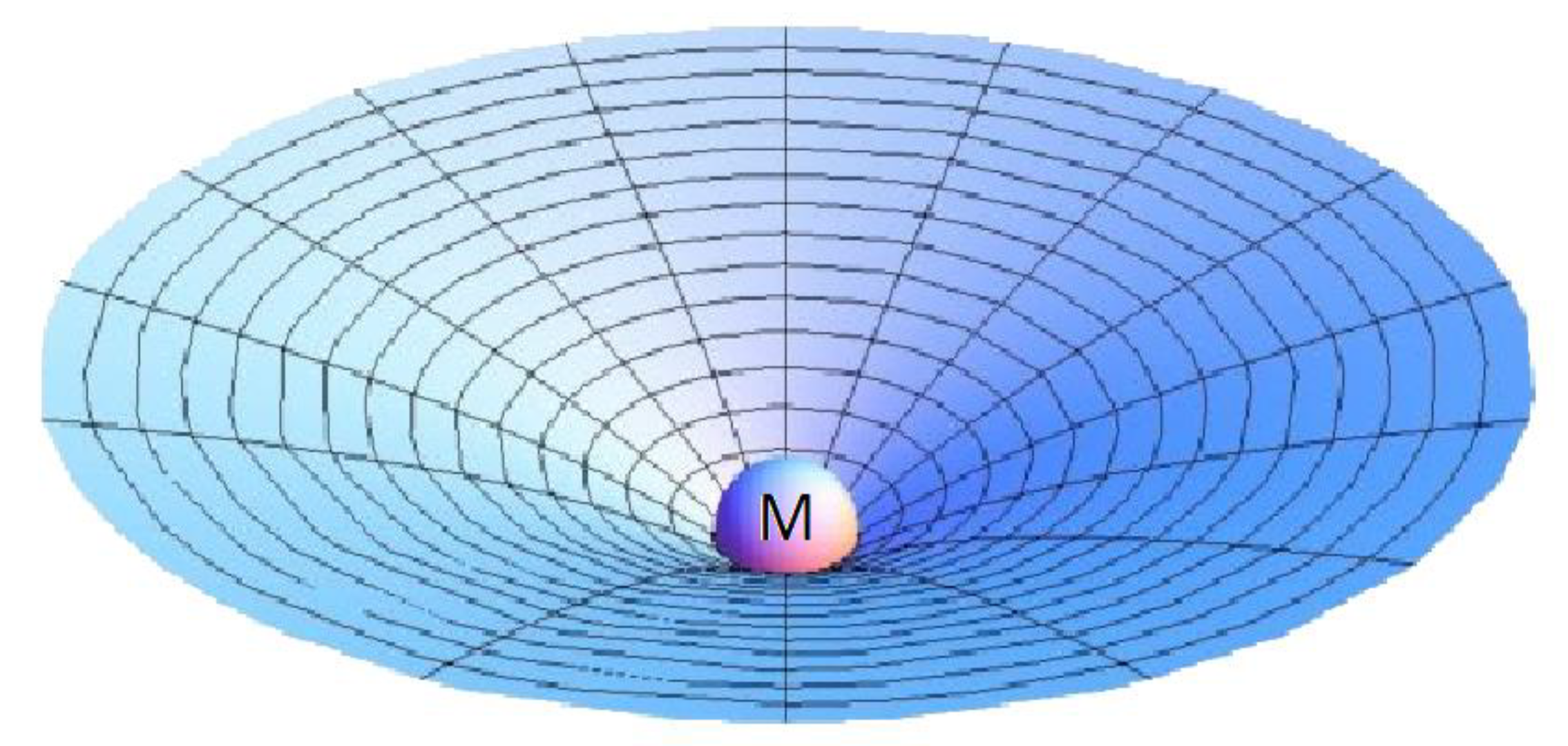
By analogy, let us imagine that our universe is confined to the surface of a 2D sphere embedded in 3D space. In the presence of massive objects, such as stars or galaxies, this surface will undergo local deformations. These deformations, in the weak field limit, can be modeled by the Schwarzschild metric. Restricting to a 2D section, the embedding of this metric in 3D Euclidean space results in the well-known Flamm's paraboloid.

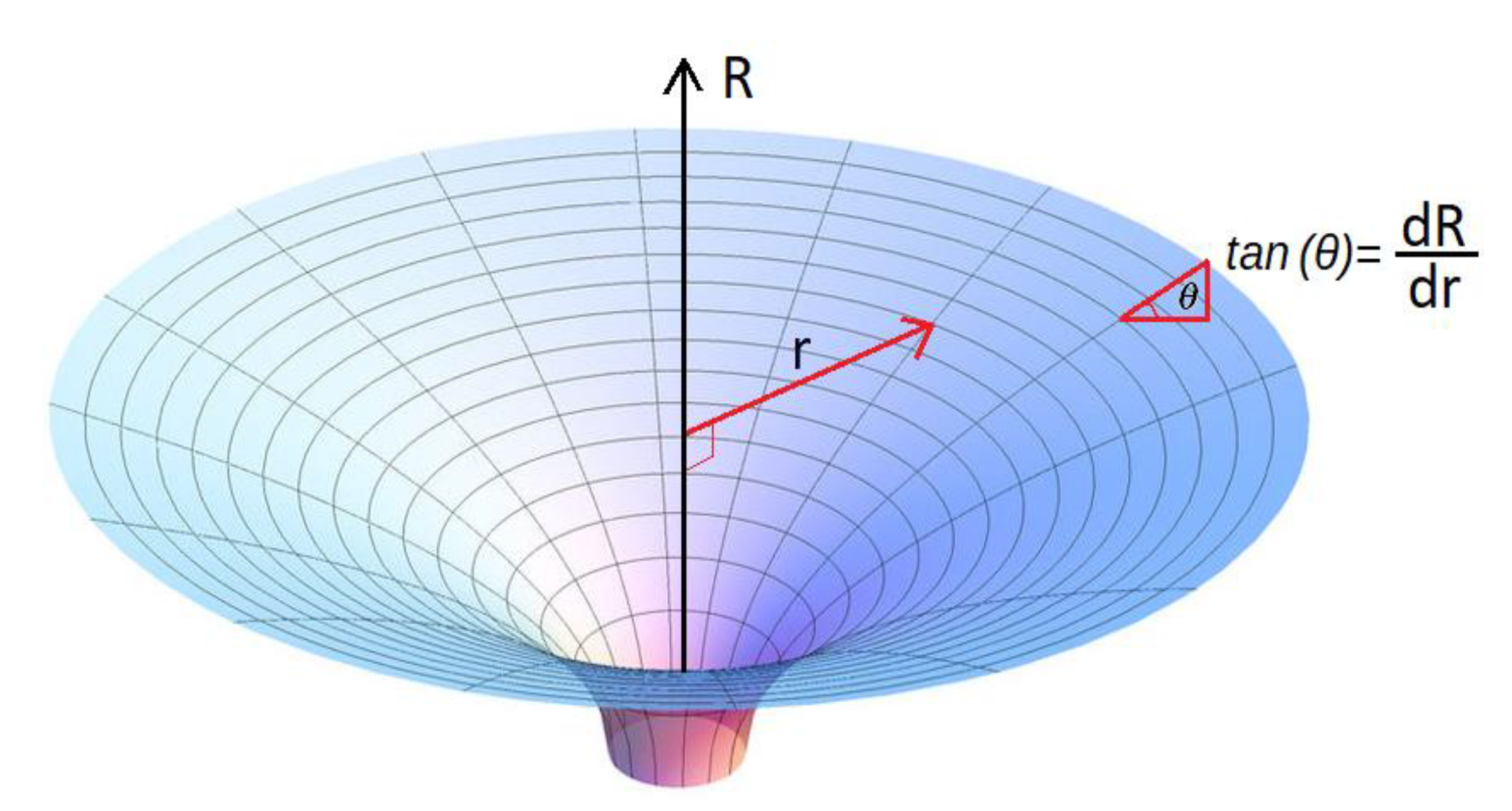
If we assume the above as correct, we may consider that part of the cosmological acceleration g_C(τ) could be projected into the radial coordinate r, affected by the slope of the paraboloid. To do this, it is enough to multiply g_C(τ) by sin(θ) where θ is the angle between the tangent to the paraboloid and the equatorial plane, as shown in the figure below.

From Flamm’s paraboloid, the slope at each point r is:

$$\mathrm{t}\mathrm{a}\mathrm{n}(\theta )={\displaystyle \frac{dR\left(\tau \right)}{dr}}=\sqrt{g_{rr}(r)-1}=\sqrt{{\displaystyle \frac{R_S}{r-R_S}}}$$

(192)

where R_S is now the Schwarzschild radius generated by the mass M_g located at r = 0:

$$R_s={\displaystyle \frac{2G{M}_g}{c^2}}$$

(193)

and g_rr(r) is the radial component of the metric.

Figure 5. Flamm's paraboloid in a 2D universe.

Figure 5. Flamm's paraboloid in a 2D universe.

For r much bigger than R_S (let's think that the mass M necessary to obtain a R_S of 1 Kpc would be of M > 1·10¹⁶ solar masses) we can approximate:

$$\mathrm{s}\mathrm{i}\mathrm{n}(\theta )\simeq \tan \left(\theta \right)$$

(194)

Therefore, the projected acceleration becomes:

$$g_r(\tau )=\sin (\theta )g_C(\tau )\simeq {\displaystyle \frac{dR(\tau )}{dr}}{g}_C(\tau )=\sqrt{g_{rr}-1}\cdot g_C(\tau )=\sqrt{{\displaystyle \frac{R_s}{r-R_s}}}\cdot {\displaystyle \frac{-G{M}_U}{R^2(\tau )}}$$

(195)

an expression that for r much greater than R_S can be approximated to:

$$g_r\left(r\right)\simeq \sqrt{{\displaystyle \frac{R_s}{r}}}\cdot {\displaystyle \frac{-G{M}_u}{R_U^2}}$$

(196)

where we have assumed that the universe ratio, R(τ), remains approximately constant, so we have defined R_U = R(τ).

Figure 6. Diagram with the tan(θ) in a Flamm paraboloid.

Figure 6. Diagram with the tan(θ) in a Flamm paraboloid.

Now we write the condition of centripetal balance for an object of mass m rotating in a circular orbit at distance r:

$$\mathrm{m}{\displaystyle \frac{v^2\left(r\right)}{r}}=\mathrm{m}\cdot g_N\left(r\right)+\mathrm{m}\cdot g_r\left(r\right)={\displaystyle \frac{G{M}_{g}m}{r^2}}+\mathrm{m}\sqrt{{\displaystyle \frac{R_s}{r}}}\cdot {\displaystyle \frac{G{M}_U}{R_U^2}}$$

(197)

where g_N(r) is the acceleration of gravity according to Newton.

If now, for very large r, we ignore the part due to Newton's acceleration of gravity since it has a dependence on 1/r² compared to the dependence 1/r^1/2 of the second summation, we will obtain what we can define as cosmological velocity, v_C(r):

$$v_C^2\left(r\right)=r\cdot g_r(r)=\sqrt{{\displaystyle \frac{R_s}{r}}}\cdot {\displaystyle \frac{G{M}_U}{R_U^2}}\mathrm{r}={\displaystyle \frac{G{M}_U}{R_U^2}}\sqrt{R_{s}r}=g_C\left(\mathsf{\tau }\right)\sqrt{R_{s}r}$$

(198)

And if we take the square root to obtain v_C(r):

$$v_C\left(r\right)=\sqrt{g_C\left(\tau \right)}\cdot \sqrt[4]{R_{s}r}$$

(199)

Subtituting the value of R_S of equation (193) we get:

$${\mathrm{v}}_{\mathrm{C}}\left(\mathrm{r}\right)=\sqrt{{\mathrm{g}}_{\mathrm{C}}\left(\mathsf{\tau }\right)}\cdot \sqrt[4]{r{\displaystyle \frac{2G{M}_g}{c^2}}}=\sqrt{{\displaystyle \frac{G{M}_U}{R_U^2}}}\cdot \sqrt[4]{r{\displaystyle \frac{2G{M}_g}{c^2}}}$$

(200)

From here, we can solve for the galaxy mass M_g:

$${\mathrm{M}}_{\mathrm{g}}=v_C^4\cdot {\displaystyle \frac{c^2{R}_U^4}{2G^3{M}_U^{2}r}}$$

(201)

that is, M_g is proportional to:

$${\mathrm{M}}_{\mathrm{g}}\propto {\displaystyle \frac{v_c^4}{r}}\propto v_c^4$$

(202)

The expression (202) shows that the mass of a galaxy is proportional to the fourth power of the rotation velocity v_c(r), which is the essence of the Tully-Fisher relation 8. However, an undesired residual dependence on the radial coordinate r remains. This is due to the fact that the velocity expression in (200) grows as r^1/4 instead of tending to a constant.

7.1. Formal Derivation of the Cosmological Acceleration Projected onto the 3D Universe

Although the explanation in the previous section is highly visual and intuitive, it is necessary to demonstrate, mathematically and via the metric, that the radial acceleration indeed includes a term generated by the cosmological acceleration.

To do so, we start with the following form of our metric, equation (15), where we have simply replaced the radial variable r with ρ:

$$d{s}^2=c^{2}d{t}^2-d{R}^2-R^2({\displaystyle \frac{d{\rho }^2}{1-k{\rho }^2}}+{\rho }^{2}d{\theta }^2+{\rho }^{2}si{n}^2\theta d{\mathsf{\varphi }}^2)$$

(203)

Since R is the radius of the 3-sphere and plays the role of a scale factor, we define:

$$r=R\rho$$

(204)

so that the 5D metric becomes:

$$d{s}^2=c^{2}d{t}^2-d{R}^2-{\displaystyle \frac{d{r}^2}{1-k\frac{r^2}{R^2}}}-r^{2}d{\mathsf{\Omega }}^2$$

(205)

In this expression, r now has dimensions of length and is scaled by R (with r < R by definition).

The next step is to derive from this metric an expression analogous to the Schwarzschild metric, including the gravitational effects generated by a mass m located at r = 0.

Following the same reasoning as at the beginning of this work, we now suppose that the radius of the 3-sphere depends on both time t and the radial coordinate r, that is:

$$dR={\displaystyle \frac{\partial R}{\partial t}}dt+{\displaystyle \frac{\partial R}{\partial r}}dr$$

(206)

We allow R = R(t,r) to reflect deviations from perfect homogeneity due to local mass-energy concentrations, encoded through the Schwarzschild perturbation around r = 0. This describes the embedding of local gravitational effects within a globally curved 5D hypersphere.

The second term in dR multiplying dr corresponds precisely to the slope of the Flamm paraboloid, as obtained previously in equation (192), where g_rr is the Schwarzschild component:

$${\displaystyle \frac{\partial R}{\partial r}}=\sqrt{g_{rr}-1}$$

(207)

By squaring dR and substituting into the metric, we obtain:

$$d{s}^2=c^{2}d{t}^2-{\displaystyle \frac{d{r}^2}{1-k\frac{r^2}{R^2}}}-r^{2}d{\mathsf{\Omega }}^2-\dot{R^2}d{t}^2-(g_{rr}-1)d{r}^2-2\dot{R}\sqrt{g_{rr}-1}\cdot drdt$$

(208)

Rearranging terms:

$$d{s}^2=(1-{\displaystyle \frac{\dot{R^2}}{c^2}})c^{2}d{t}^2-({\displaystyle \frac{1}{1-\frac{r^2}{R^2}}}+g_{rr}-1)d{r}^2-r^{2}d{\Omega }^2-2\dot{R}\sqrt{g_{rr}-1}\cdot drdt$$

(209)

Now, defining proper time as:

$$d\tau =\sqrt{1-{\displaystyle \frac{\dot{R^2}}{c^2}}}dt$$

(210)

and noting that:

$$\dot{R}(t)dt={\displaystyle \frac{dR(t)}{dt}}dt={\displaystyle \frac{dR(t)}{d\tau }}{\displaystyle \frac{d\tau }{dt}}dt=\dot{R}(\tau )d\tau$$

(211)

we get:

$$d{s}^2=c^{2}d{\tau }^2-({\displaystyle \frac{1}{1-k\frac{r^2}{R^2}}}+g_{rr}-1)d{r}^2-r^{2}d{\mathsf{\Omega }}^2-2\dot{R}(\tau )\sqrt{g_{rr}-1}\cdot drd\tau$$

(212)

Lastly, we account for the time dilation due to the gravitational field by introducing the g_tt factor multiplying dτ²:

$$d{s}^2=g_{tt}d{\tau }^2-({\displaystyle \frac{1}{1-k\frac{r^2}{R^2}}}+g_{rr}-1)d{r}^2-r^{2}d{\mathsf{\Omega }}^2-2\dot{R}(\tau )\sqrt{g_{rr}-1}\cdot drd\tau$$

(213)

And finally, taking the limit r << R and re-identifying dt = dτ, we arrive at the effective metric:

$$d{s}^2=g_{tt}d{t}^2-g_{rr}d{r}^2-r^{2}d{\Omega }^2-2\dot{R}(t)\sqrt{g_{rr}-1}\cdot drdt$$

(214)

Here, g_tt and g_rr are the standard Schwarzschild metric components, and a new cross term appears:

$$g_{rt}=\dot{R}(t)\sqrt{g_{rr}-1}$$

(215)

Thus, we obtain a modified Schwarzschild-like metric of the form:

$$d{s}^2=(1-{\displaystyle \frac{R_s}{r}})c^{2}d{t}^2-{\displaystyle \frac{d{r}^2}{(1-\frac{R_s}{r})}}-r^{2}d{\Omega }^2-2\dot{R}\sqrt{{\displaystyle \frac{R_s}{r-R_s}}}drdt$$

(216)

• Radial Acceleration of an Orbiting Observer

Now, once we have obtained the above form of the metric with the new cross term g_rt, we must now check that this cross term is the cause of the cosmological acceleration g_r(r).

Let us consider an observer in circular motion in the equatorial plane (sin θ = 1) around a central mass M_g that generates the gravitational field. This implies that dr = dθ = 0, and hence the four-velocity of the observer is:

$$u^{\mu }={\displaystyle \frac{d{x}^{\mu }}{d\tau }}=({\displaystyle \frac{dt}{d\tau }},{\displaystyle \frac{dr}{d\tau }},{\displaystyle \frac{d\theta }{d\tau }},{\displaystyle \frac{d\varphi }{d\tau }})=({\displaystyle \frac{dt}{d\tau }},\mathrm{0,0},{\displaystyle \frac{d\varphi }{d\tau }})$$

(217)

Defining the angular velocity as:

$$\omega ={\displaystyle \frac{d\varphi }{dt}}$$

(218)

we can express the four-velocity as:

$$u^{\mu }=({\displaystyle \frac{dt}{d\tau }},\mathrm{0,0},\omega {\displaystyle \frac{dt}{d\tau }})=(u^t,\mathrm{0,0},\omega \cdot u^t)$$

(219)

We now compute the radial component of the four-acceleration:

$$a^r={\displaystyle \frac{d{u}^r}{d\tau }}+{\Gamma }_{\alpha \beta }^r{u}^{\alpha }{u}^{\beta }$$

(220)

Since u^r = 0 and u^θ = 0, the first term and all the terms with u^r or u^θ vanish. If we also consider only the non-zero Christoffel symbols relevant for the radial direction, we finally obtain:

$$a^r={\Gamma }_{tt}^r(u^t{)}^2+{\Gamma }_{\varphi \varphi }^r(u^{\varphi }{)}^2$$

(221)

We now compute the Christoffel symbols. Starting with Γ_tt^r:

$${\mathsf{\Gamma }}_{tt}^r={\displaystyle \frac{1}{2}}{g}^{rr}({\partial }_t{g}_{tr}+{\partial }_t{g}_{rt}-{\partial }_r{g}_{tt})+{\displaystyle \frac{1}{2}}{g}^{tr}({\partial }_t{g}_{tt}+{\partial }_t{g}_{tt}-{\partial }_t{g}_{tt})$$

(222)

Since g_tt does not depend on time, the second term vanishes, and we obtain:

$${\Gamma }_{tt}^r={\displaystyle \frac{1}{2}}{g}^{rr}(2\ddot{R}\sqrt{g_{rr}-1}-{\partial }_r{g}_{tt})$$

(223)

Using the Schwarzschild relation for the Newtonian acceleration:

$${\partial }_r{g}_{tt}=-2g_N(r)$$

(224)

we find:

$${\Gamma }_{tt}^r={\displaystyle \frac{1}{2}}{g}^{rr}(2\ddot{R}\sqrt{g_{rr}-1}+2g_N(r))$$

(225)

Now, we compute the angular Christoffel symbol:

$${\Gamma }_{\varphi \varphi }^r={\displaystyle \frac{1}{2}}{g}^{rr}({\partial }_{\varphi }{g}_{\varphi r}+{\partial }_{\varphi }{g}_{r\varphi }-{\partial }_r{g}_{\varphi \varphi })=-g^{rr}\cdot r$$

(226)

Putting all terms together:

$$a^r={\displaystyle \frac{1}{2}}{g}^{rr}(2\ddot{R}\sqrt{g_{rr}-1}+2g_N(r)-2r{\omega }^2)(u^t{)}^2$$

(227)

Finally, assuming the observer is in free fall and thus follows a geodesic (a^r = 0), we obtain:

$$\ddot{R}\sqrt{g_{rr}-1}+g_N(r)=r{\omega }^2={\displaystyle \frac{r^2{\omega }^2}{r}}={\displaystyle \frac{v^2}{r}}$$

(228)

Recall from equation (86) that we had defined the cosmological acceleration in the extra dimension R as:

$$g_C\left(\tau \right)\equiv \ddot{R}\left(\tau \right)=-{\displaystyle \frac{G{M}_U}{R^2\left(\tau \right)}}$$

(86)

which represents a Newtonian-like deceleration in the hyperspherical expansion, consistent with a closed universe without dark energy.

Substituting into the previous result, we finally recover:

$${\displaystyle \frac{v^2}{r}}=g_N(r)+g_C(\tau )\sqrt{g_{rr}-1}=g_N(r)+g_r(r)$$

(229)

that is, we recover equation (197), which expresses the total radial acceleration of an object in circular orbit as the sum of the Newtonian term and a new term g_r(r) resulting from the projection of the cosmological acceleration through the slope of the Flamm-like embedding in 5D and whose value coincides with that of expression (195) as we wanted to demonstrate.

7.2. Alternative to the Einstein-Strauss Vacuole: The Emergent Negative Mass And Its effect

According to Birkhoff’s theorem, the only spherically symmetric solution to Einstein’s field equations in vacuum is the Schwarzschild metric. In the Einstein–Strauss construction 10, this solution was embedded within the FLRW background by defining a “vacuole”: a comoving spherical region around the central mass M_g, with radius R_v chosen such that the mass enclosed in the corresponding FLRW sphere matches the mass of the object (galaxy, cluster, etc.) represented by the Schwarzschild metric. The matching condition is:

$$M_g={\displaystyle \frac{4}{3}}\pi R_v^3{\rho }_u$$

(230)

where ρ_U is the average density of the universe. Solving for R_v:

$$R_v=\sqrt[3]{{\displaystyle \frac{M_g}{M_U}}}\cdot R_U$$

(231)

In this work, as an alternative to the Einstein–Strauss vacuole, we propose modifying the radial metric component g_rr(r) so that it induces an effective negative mass density that partially screens the baryonic source mass. The hypothesis is that the geometry of the hypersphere deforms in such a way that it compensates the gravitational mass M_g by generating an effective negative contribution, such that the net density is reduced.

Specifically, we consider:

$$g_{rr}(r)={\displaystyle \frac{1}{1-\frac{Rs}{r}(1-f(r){)}^n}}$$

(232)

where f(r) satisfies f(0) = 0, f(r→∞)→1. For small r, the metric reduces to the Schwarzschild form, while for large r the slope of the Flamm paraboloid is suppressed. The parameter n controls how the effective circular velocity scales with radius; observations consistent with the Tully–Fisher relation (flat curves beyond ∼1 Mpc) require n=1, yielding:

$$g_{rr}(r)={\displaystyle \frac{1}{1-\frac{Rs}{r}(1-f(r))}}$$

(233)

If we also set g_tt(r) = 1/g_rr(r), the Einstein equations give:

$$G_t^t=-{\displaystyle \frac{R_S}{r^2}}{\displaystyle \frac{df(r)}{dr}}=T_t^t={\displaystyle \frac{8\pi G}{c^2}}\rho (r)$$

(234)

which implies an effective negative mass density:

$$\rho (r)=-{\displaystyle \frac{R_S}{r^2}}{\displaystyle \frac{df(r)}{dr}}{\displaystyle \frac{c^2}{8\pi G}}$$

(235)

We can now compute the total mass enclosed within a radius r′ using the expression:

$$M(r\text{'})={\int }_0^{r\text{'}}4\pi r^2\rho (r)dr=-{\int }_0^{r\text{'}}{\displaystyle \frac{4\pi r^2}{r^2}}{\displaystyle \frac{R_S{c}^2}{8\pi G}}{\displaystyle \frac{df(r)}{dr}}dr={\displaystyle \frac{-R_S{c}^2}{2G}}{\int }_0^{r\text{'}}df(r)={\displaystyle \frac{-R_S{c}^2}{2G}}[f(r\text{'})-f(0)]$$

(236)

and using the definition of R_S (Eq. (193)) with f(0)=0:

$$M(r)=-M_g\cdot f(r)$$

(237)

Thus, the effective mass reduces the source mass by a fraction f(r′), screening the net gravitational field. Since f(r→∞) = 1, the negative contribution asymptotically approaches—but never exactly cancels—the baryonic mass.

This emergent negative mass density should not be interpreted as a real negative matter component in the universe, but as a geometric screening effect: the deformation of local spacetime reduces the slope of the Flamm paraboloid, which weakens the effective gravity at large radii and naturally explains flat galactic rotation curves without invoking dark matter. Crucially, the local mass density remains positive everywhere; the “negative mass effect” is simply a manifestation of the modified geometry.

7.2.1. Modification of the Local Metric

Starting from the modified Schwarzschild metric of (216):

$$d{s}^2=(1-{\displaystyle \frac{R_s}{r}})c^{2}d{t}^2-{\displaystyle \frac{d{r}^2}{(1-\frac{R_s}{r})}}-r^{2}d{\Omega }^2-2\dot{R}\sqrt{{\displaystyle \frac{R_s}{r-R_s}}}drdt$$

(238)

we propose modifying g_rr(r) using the following expression for f(r):

$$f(r)={\displaystyle \frac{r}{r+r_0}}$$

(239)

so that:

$$g_{rr}(r)={\displaystyle \frac{1}{1-\frac{R_s}{r}(1-f(r))}}={\displaystyle \frac{1}{1-\frac{R_s}{r}(1-\frac{r}{r+r_o})}}={\displaystyle \frac{1}{1-\frac{R_s}{r}(\frac{r_o}{r+r_o})}}$$

(240)

where r_o is a scale parameter whose value depends on the particular characteristics of each galaxy. This choice of f(r) is not derived from first principles but is proposed for its simplicity, which facilitates the calculations in the following sections. Future work may explore alternative forms of g_rr(r), possibly derived from junction conditions or from matching to full McVittie-type metrics in 5D.

We now define the parameter k_v as:

$$r_o={\displaystyle \frac{R_v}{k_v}}$$

(241)

where R_v is the vacuole radius defined in (254). The function f(r) then takes the form:

$$f(r)={\displaystyle \frac{r}{r+R_v/k_v}}={\displaystyle \frac{k_{v}r}{k_{v}r+R_v}}$$

(242)

Substituting this into the previous expression yields:

$$g_{rr}(r)={\displaystyle \frac{1}{1-\frac{R_s}{r}(\frac{r_o}{r+r_o})}}={\displaystyle \frac{1}{1-\frac{R_s}{r}(\frac{R_v}{k_{v}r+R_v})}}$$

(243)

The slope of the Flamm paraboloid is then:

$${\displaystyle \frac{dR(\tau )}{dr}}={\displaystyle \frac{d{R}_U}{dr}}=\sqrt{g_{rr}(r)-1}=\sqrt{{\displaystyle \frac{R_s{r}_o}{r\left(r+r_o\right)-R_s{r}_o}}}\simeq \sqrt{{\displaystyle \frac{R_s{r}_o}{r\left(r+r_o\right)}}}=\sqrt{{\displaystyle \frac{R_s{R}_v}{r\left(k_v\cdot r+R_v\right)}}}$$

(244)

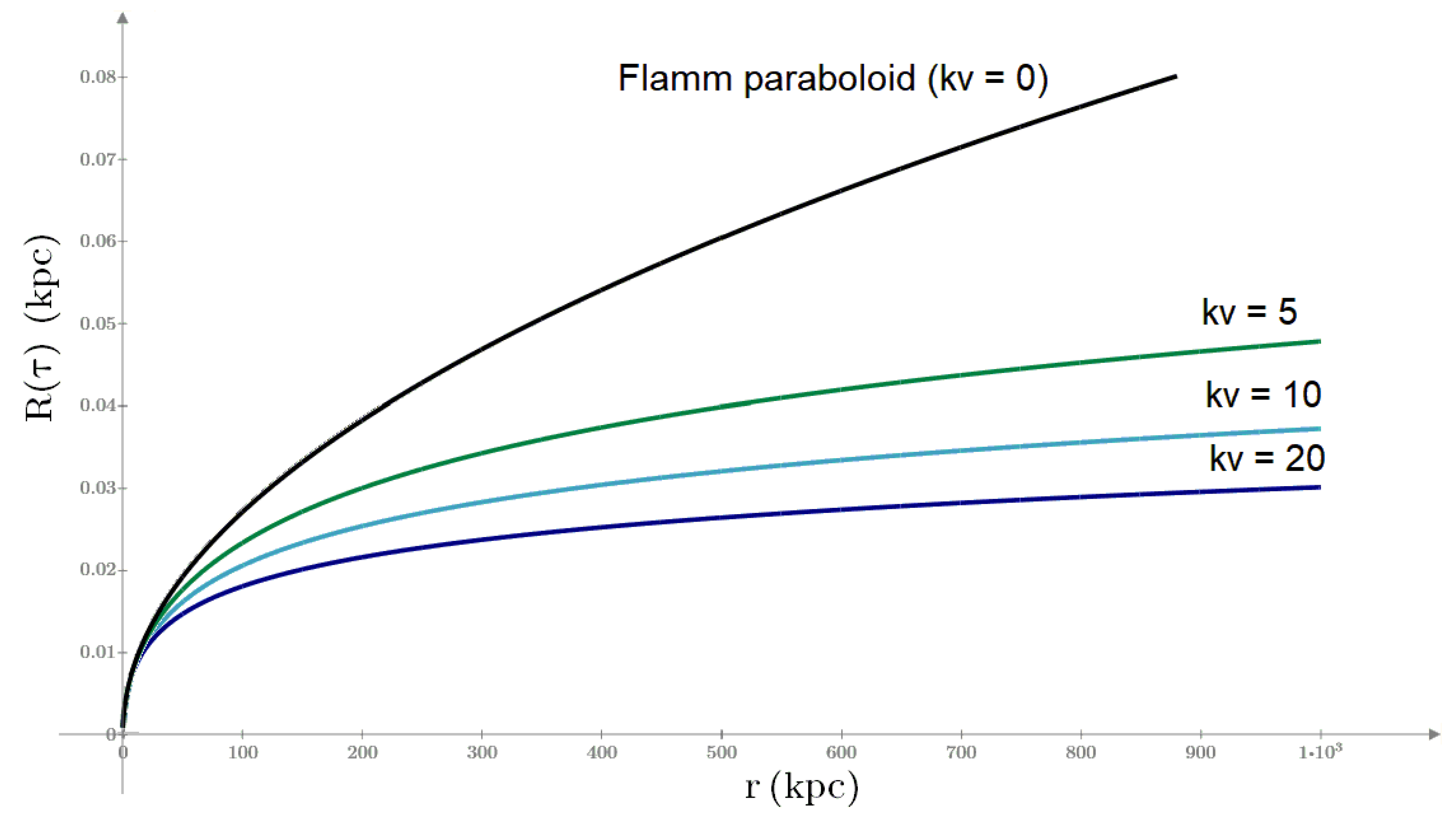
Integrating with respect to r, we obtain the approximate form of the paraboloid:

$$R(\tau )=R_U(r)\simeq -2\sqrt{{\displaystyle \frac{Rs{R}_v}{k_v}}}\ln ({\displaystyle \frac{\sqrt{k_{v}r+R_v}-\sqrt{k_{v}r}}{\sqrt{k_v{R}_s+R_v}-\sqrt{k_v{R}_s}}})$$

(245)

This allows us to graph (next figure) the shape of the paraboloid and see how it changes with different values of k_v.

If we substitute f(r) into expression (239) for the effective negative mass, we obtain:

$$M(r)=-M_g{\displaystyle \frac{k_{v}r}{k_{v}r+R_v}}$$

(246)

where M_g is the baryonic mass of the central object. Once R_v is identified with the Einstein–Straus vacuole radius, the negative mass enclosed within R_v is:

$$\mathrm{M}({\mathrm{R}}_{\mathrm{v}})=-{\mathrm{M}}_{\mathrm{g}}{\displaystyle \frac{{\mathrm{k}}_{\mathrm{v}}{\mathrm{R}}_{\mathrm{v}}}{{\mathrm{k}}_{\mathrm{v}}{\mathrm{R}}_{\mathrm{v}}+{\mathrm{R}}_{\mathrm{v}}}}=-{\mathrm{M}}_{\mathrm{g}}{\displaystyle \frac{{\mathrm{k}}_{\mathrm{v}}}{{\mathrm{k}}_{\mathrm{v}}+1}}<-{\mathrm{M}}_{\mathrm{g}}$$

(247)

which is always less than −M_g, with equality only in the limit k_v → ∞. For example, if we take k_v = 5, which—as shown later—provides the best fit to galactic rotation curves, the negative mass enclosed within the vacuole is about 83.3% of M_g.

Thus, the parameter k_v governs the reduction of the paraboloid slope and the amount of effective negative mass −M(r) enclosed within R_v. A higher k_v corresponds to a shallower slope and a larger effective screening mass.

Figure 7. Flamm's Paraboloide in function of k_v.

Figure 7. Flamm's Paraboloide in function of k_v.

Finally, he expression for the projected cosmological acceleration becomes:

$$g_r(r)=g_c(\tau )\sqrt{g_{rr}(r)-1}={\displaystyle \frac{-G{M}_U}{R_U^2}}\sqrt{{\displaystyle \frac{R_s{r}_o}{r(r+r_o)-R_s{r}_o}}}={\displaystyle \frac{-G{M}_U}{R_U^2}}\sqrt{{\displaystyle \frac{R_s{R}_v}{r(k_{v}r+R_v)-R_s{R}_v}}}$$

(248)

For r >> R_s, we can approximate this as:

$$g_r(r)={\displaystyle \frac{-G{M}_U}{R_U^2}}\sqrt{{\displaystyle \frac{R_s{R}_v}{r(k_{v}r+R_v)}}}$$

(249)

We can now use (248) to compute the cosmological velocity as:

$$v_C^2\left(r\right)=r\cdot g_r(r)={\displaystyle \frac{G\cdot M_U\cdot r}{R_U^2}}\sqrt{{\displaystyle \frac{R_s{r}_o}{r\left(r+r_o\right)-R_s{r}_o}}}=g_C\left(\tau \right)\cdot \sqrt{{\displaystyle \frac{r^2{R}_s{R}_v}{r\left(k_{v}r+R_v\right)-R_s{R}_v}}}$$

(250)

Taking the square root again gives:

$$v_C\left(r\right)=\sqrt{g_C\left(\tau \right)}\cdot \sqrt[4]{{\displaystyle \frac{r^2{R}_s{R}_v}{r\left(k_{v}r+R_v\right)-R_s{R}_v}}}$$

(251)

For r >> R_S, we can approximate this as:

$$v_C\left(r\right)=\sqrt{g_C\left(\tau \right)}\cdot \sqrt[4]{{\displaystyle \frac{r{R}_s{R}_v}{k_{v}r+R_v}}}$$

(252)

And in the limit r·k_v >> R_v, this tends toward a constant value:

$$v_C(r)=\sqrt{g_C(\tau )}\cdot \sqrt[4]{{\displaystyle \frac{R_s{R}_v}{k_v}}}$$

(253)

Thus, the dependence on r^1/4 that appeared in equation (200) is effectively eliminated.

Therefore, to conclude this section, and assuming—as is commonly done—that the temporal and radial components of the metric satisfy the condition g_tt = c²/g_rr, the new modified Schwarzschild-like metric takes the form:

$$d{s}^2=(1-{\displaystyle \frac{R_s}{r}}\cdot {\displaystyle \frac{R_v}{k_{v}r+R_v}})c^{2}d{t}^2-{\displaystyle \frac{d{r}^2}{1-\frac{R_s}{r}\cdot \frac{R_v}{k_{v}r+R_v}}}-r^{2}d{\mathsf{\Omega }}^2-2\dot{R}(\tau )\sqrt{{\displaystyle \frac{R_s{R}_v}{r\left(k_v\cdot r+R_v\right)}}}drdt$$

(254)

This expression encapsulates the proposed deformation of the Schwarzschild geometry due to the projected cosmological acceleration. The additional cross term g_tr encodes the influence of the 5D cosmological dynamics on the 4D spacetime structure. The modification of the therm g_rr effectively flattens the Flamm paraboloid at large distances, allowing for the smooth embedding of local Schwarzschild vacuoles within the globally curved 3-sphere geometry of the universe.

To complete the derivation, we now reintroduce the terms that were previously neglected, and revert the time substitution dt = dτ, obtaining:

$$d{s}^2=(1-{\displaystyle \frac{R_s}{r}}\cdot {\displaystyle \frac{R_v}{k_{v}r+R_v}})c^{2}d{\tau }^2-({\displaystyle \frac{1}{1-\frac{r^2}{R_U^2(\tau )}}}+{\displaystyle \frac{1}{1-\frac{R_s}{r}\cdot \frac{R_v}{k_{v}r+R_v}}}-1)d{r}^2-r^{2}d{\Omega }^2-2\dot{R}(\tau )\sqrt{{\displaystyle \frac{R_s{R}_v}{r\left(k_v\cdot r+R_v\right)-R_s{R}_v}}}\cdot drd\tau$$

(255)

Finally, we express the metric in terms of the coordinate time by using equation (54) with k = 1,

$$d\tau =\sqrt{{\displaystyle \frac{R^2(ct)}{R_{sU}(R_R+R(ct))}}}\cdot dt$$

(54)

where R_SU is the Schwarzschild radius of the universe (given by equation (49)). Now, previous equation can be approximated, for a universe dominated by matter, as:

$$d\tau =\sqrt{{\displaystyle \frac{R(ct)}{R_{SU}}}}\cdot dt$$

(256)

and by substituting the expression for $\dot{R}(t)$ from equation (51) for k = 1 and R(t) >> R_R, we arrive at the general form of the metric:

$$d{s}^2=(1-{\displaystyle \frac{R_s}{r}}\cdot {\displaystyle \frac{R_v}{k_{v}r+R_v}}){\displaystyle \frac{R(t)}{R_{SU}}}{c}^{2}d{t}^2-({\displaystyle \frac{1}{1-\frac{r^2}{R^2(t)}}}+{\displaystyle \frac{1}{1-\frac{R_s}{r}\cdot \frac{R_v}{k_{v}r+R_v}}}-1)d{r}^2-r^{2}d{\mathsf{\Omega }}^2-2c\sqrt{(1-{\displaystyle \frac{R(t)}{R_{SU}}}){\displaystyle \frac{R_s{R}_v}{r\left(k_v\cdot r+R_v\right)-R_s{R}_v}}}\cdot drdt$$

(257)

Equation (257) represents one of the central results of this work: a generalized metric that consistently merges local gravitational fields with the global cosmological evolution dictated by the expansion of the hyperspherical radius R(t) for a matter dominated universe. Unlike standard Schwarzschild or FLRW metrics—which separately describe local and global structures—this expression provides a unified spacetime geometry incorporating both contributions in a fully geometric and covariant framework.

Structurally, this metric can be seen as a natural analogue to the McVittie metric, which was originally formulated to embed a central mass within an expanding cosmological background. However, in the present model, the coupling between local mass distributions and global dynamics arises not from an ansatz or continuity condition, but from a consistent projection of the 5D cosmological geometry onto the 4D spacetime through the Flamm paraboloid's deformation and the time evolution of R_U(t). The presence of the cross term g_tr is not postulated, but instead derived as a geometric consequence of the embedding structure.

This formulation confirms and justifies the effective acceleration term g_C previously introduced on heuristic grounds. It also allows for a more rigorous treatment of the rotational dynamics of galaxies, the Tully–Fisher relation, and the cosmological redshift, all within the same metric foundation. Furthermore, the metric reduces to known cases in the appropriate limits: the Schwarzschild geometry is recovered for R_U(t)→ const, and a modified FLRW form emerges in the weak-field regime or at cosmological scales where local mass terms become negligible.

As such, equation (257) constitutes the foundational spacetime structure from which the model's dynamical and observational predictions can be coherently derived.

7.2.2. Modification of the Newtonian Acceleration

In this section, we analyze how the modified form of the Schwarzschild metric, given by equation (254), affects the expression for gravitational acceleration. Specifically, we compute the Newtonian radial acceleration using the g_tt(r) component of the metric. A minus sign is introduced to indicate that the gravitational force is attractive, i.e., directed toward the origin of coordinates:

$$g_N(r)=-{\displaystyle \frac{1}{2}}{\partial }_r{g}_{tt}$$

(258)

This leads to the expression:

$$g_N\left(r\right)=-{\displaystyle \frac{GM}{r^2}}\left(1-{\left({\displaystyle \frac{k_{v}r}{k_{v}r+R_v}}\right)}^2\right)$$

(259)

As a result, the gravitational acceleration is no longer determined solely by the local mass, but is modified by the influence of the global geometry—specifically, the coupling between the local paraboloid structure and the curvature of the higher-dimensional hypersphere.

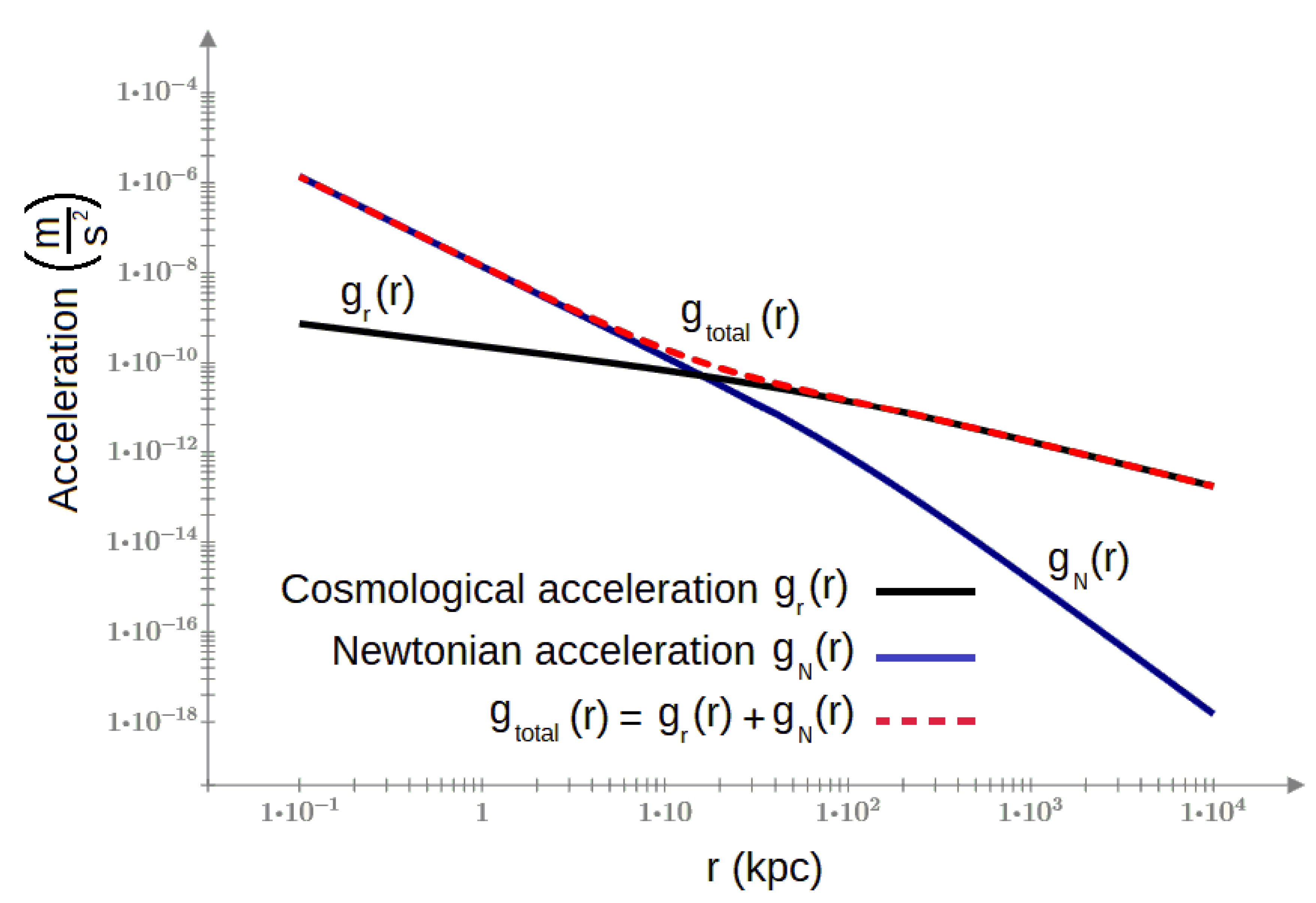
Finally, the next figure shows comparison of the Newtonian acceleration (g_N, blue line) and the projected cosmological acceleration (g_r, black line) for a typical galaxy with a baryonic mass of M_g = 10¹¹ M_☉. The Newtonian acceleration dominates at small radii, while the cosmological acceleration becomes dominant at r > 10 kpc, explaining the observed dynamics without the need for dark matter, as we will show later. The dashed red line shows the total acceleration (g_total = g_N + g_r).

Figure 2. Comparison of the Newtonian acceleration and cosmological acceleration.

Figure 2. Comparison of the Newtonian acceleration and cosmological acceleration.

7.3. Derivation of the Mass–Velocity Relation

Previously, in equation (202), we found that M_g ∝ v⁴, in full agreement with the Tully–Fisher relation. In this section, we will examine whether the inclusion of R_v — defined as the vacuole radius — and thus its dependence on M_g, modifies this proportionality relation. Let us analyze this:

If we raise equation (253), which gives v_C(r) for r >> R_v, to the fourth power, we obtain:

$$v_C^4(r)=g_C^2(\tau )\cdot {\displaystyle \frac{R_s{R}_v}{k_v}}$$

(260)

Using the definition of R_v from equation (231), we have:

$$v_C^4\left(r\right)=g_C^2\left(\tau \right){\displaystyle \frac{R_s}{k_v}}\cdot \sqrt[3]{{\displaystyle \frac{Mg}{M_U}}}\cdot R_U$$

(261)

Now, substituting the expression for R_s from equation (198), we obtain:

$$v_C^4\left(r\right)=g_C^2\left(\mathsf{\tau }\right){\displaystyle \frac{2G{M}_g}{c^2}}\sqrt[3]{{\displaystyle \frac{M_g}{M_U}}}\cdot {\displaystyle \frac{R_U}{k_v}}=g_C^2\left(\mathsf{\tau }\right){\displaystyle \frac{2G}{c^2}}\sqrt[3]{{\displaystyle \frac{M_g^4}{M_U}}}\cdot {\displaystyle \frac{R_U}{k_v}}$$

(262)

With a bit of algebra, we can isolate the mass of the galaxy and obtain:

$${\mathrm{M}}_{\mathrm{g}}\left(\mathrm{v}\right)={\displaystyle \frac{c\cdot R_U^2}{G^2\cdot M_U}}\sqrt[4]{{\displaystyle \frac{R_U\cdot c^2\cdot k_v^3}{8\cdot G\cdot M_U}}}\cdot v_c^3$$

(263)

That is:

$${\mathrm{M}}_{\mathrm{g}}\left(\mathrm{v}\right)={\mathrm{C}}_{\mathrm{M}\mathrm{V}}\cdot v_c^3$$

(264)

where, if the velocity is in km/s and the mass in solar masses, has the value:

$$C_{MV}={\displaystyle \frac{c{R}_U^2}{G^2\cdot M_U}}\sqrt[4]{{\displaystyle \frac{R_U\cdot c^2\cdot k_v^3}{8\cdot G\cdot M_U}}}=7.25\cdot 10^3{\displaystyle \frac{M_{\odot }}{\mathrm{k}{\mathrm{m}}^3/{\mathrm{s}}^3}}$$

(265)

In summary, from equation (263) we obtain the following relation:

$$M_g(v)\propto v_c^3$$

(266)

This expression differs from the classical Tully–Fisher relation M ∝ v⁴. In addition to the change in the exponent of v_c, the new expression (263) has no dependence on the radial distance, unlike equation (201), which included a 1/r dependence, leading to a scale-invariant flat rotation curve.

In the proposed 5D framework, the baryonic Tully–Fisher relation (BTFR) naturally exhibits a scale-dependent exponent, transitioning from M ∝ v⁴ at small radii (r << R_V, where R_V denotes the vacuole radius associated with the local mass embedding) to M ∝ v³ at large radii (r >> R_V). This behavior follows directly from the projected cosmological acceleration g_r(r) derived in Eqs. (201) and (263).

Current observations, typically probing intermediate galactocentric distances (r < 100 kpc, often r < R_V for typical galaxies), yield effective exponents between 3 and 4 — for instance, 3.82 ± 0.22 in the SPARC sample 12 — in excellent agreement with the model’s prediction of intermediate values (n ≈ 3.5−3.8) a value statistically consistent with a gradual transition between the two asymptotic regimes predicted by the model.

This transitional behavior constitutes a distinctive, testable signature: future deep HI surveys, such as those to be conducted by the Square Kilometre Array (SKA), extending rotation curves to ∼1 Mpc, should reveal a gradual convergence toward the asymptotic M ∝ v³ scaling — providing a direct observational probe of the model’s geometric projection mechanism.

7.4. Derivation of MOND from Cosmological Acceleration

The hypothesis proposed in this work—that a portion of the cosmological acceleration g_C(τ) in the extra dimension R is projected onto our three-dimensional universe, generating an effective acceleration g_r(r), which in turn leads to a constant radial velocity at large distances as given by equation (253), similarly to MOND 11 enables us to explore a possible theoretical justification for the empirical MOND parameter a₀.

In the limit of large radial distances r, the previously derived expression for g_r(r) can be approximated as:

$$g_r\left(r\right)={\displaystyle \frac{-G{M}_U}{R_U^2}}\sqrt{{\displaystyle \frac{R_s{R}_v}{r\left(k_{v}r+R_v\right)-R_s{R}_v}}}\simeq {\displaystyle \frac{-G{M}_U}{R_U^2}}\sqrt{{\displaystyle \frac{R_s{R}_v}{k_v}}}\cdot {\displaystyle \frac{1}{r}}$$

(267)

On the other hand, MOND assumes that, in the very low acceleration regime, where g << a₀:

$$a_r(r)=\sqrt{G{M}_g{a}_0}\cdot {\displaystyle \frac{1}{r}}$$

(268)

Equating both expressions, we obtain:

$$\sqrt{a_{0}G{M}_g}={\displaystyle \frac{G{M}_U}{R_U^2}}\sqrt{{\displaystyle \frac{R_s{R}_v}{k_v}}}={\displaystyle \frac{G{M}_U}{R_U^2}}\sqrt{{\displaystyle \frac{2G{M}_g}{c^2{k}_v}}\cdot \sqrt[3]{{\displaystyle \frac{M_g}{M_U}}}{R}_U}$$

(269)

This allows us to isolate the MOND parameter a₀:

$$a_0={\left({\displaystyle \frac{G{M}_U}{R_U^2}}\right)}^2{\displaystyle \frac{2}{c^2{k}_v}}\cdot \sqrt[3]{{\displaystyle \frac{M_g}{M_U}}}{R}_U={\left({\displaystyle \frac{G{M}_U}{c}}\right)}^2\cdot {\displaystyle \frac{2}{k_v{R}_U}}\cdot \sqrt[3]{{\displaystyle \frac{M_g}{M_U}}}$$

(270)

which implies

$${\mathrm{a}}_0\propto \sqrt[3]{{\mathrm{M}}_{\mathrm{g}}}$$

(271)

This result is noteworthy, as some extended MOND models and emergent gravity theories have also suggested a dependence of a₀ on galaxy mass. In our model, this relation emerges naturally from the 5D spacetime geometry and the projection of the cosmological acceleration.

Finally, expression (270) enables us to estimate the value of the total mass of the universe M_U. Assuming the standard MOND value a₀ = 1.2·10^-10 m/s², and taking k_v = 5 (the value that best fits galaxy rotation curves, as will be shown later), we find that for a typical range of galactic masses M_g ∈ [1,100]·10⁹ M_⊙, the estimated total mass of the universe, using the current R_U = 4.05 × 10²⁸ m value, is:

$${\mathrm{M}}_{\mathrm{U}}\simeq \left[0.8-2\right]\cdot {10}^{60}\hspace{0.17em}\mathrm{k}\mathrm{g}$$

(272)

This value is several orders of magnitude higher than the standard estimate in the ΛCDM framework (M_U ≃1.53·10 ⁵³ kg), but it is consistent with the predictions of our 5D model, (M_U ≃1.24·10 ⁶⁰ kg) value obtained in (163) using the CMB properties .

7.5. Application to Galaxy Rotation Velocity Curves

In this section, we aim to apply the newly obtained expressions for g_N(r) and g_r(r), in order to assess whether galaxy rotation curves can be explained without resorting to dark matter.

If we write the condition for centripetal balance for an object of mass m rotating in a circular orbit at distance r from a central mass M, which generates the gravitational field, we have:

$$\mathrm{m}{\displaystyle \frac{v^2\left(r\right)}{r}}=\mathrm{m}\cdot g_N\left(\mathrm{r}\right)+\mathrm{m}\cdot g_r\left(r\right)$$

(273)

where g_N(r) is the gravitational acceleration as given by equation (259), and g_r(r) is the cosmological acceleration given by equation (248), so that:

$$v_t^2(r)=(g_N(r)+g_r(\tau ))\cdot r={\displaystyle \frac{G{M}_g}{r}}(1-({\displaystyle \frac{k_{v}r}{k_{v}r+R_v}}{)}^2)+{\displaystyle \frac{G{M}_U}{R_U^2}}\cdot \sqrt{{\displaystyle \frac{r^2{R}_s{R}_v}{r(k_{v}r+R_v)-R_s{R}_v}}}$$

(274)

For r > > Rs, this can be approximated by:

$$v_t^2(r)={\displaystyle \frac{G{M}_G}{r}}(1-({\displaystyle \frac{k_{v}r}{k_{v}r+R_v}}{)}^2)+{\displaystyle \frac{G{M}_U}{R_U^2}}\cdot \sqrt{{\displaystyle \frac{r{R}_s{R}_v}{(k_{v}r+R_v)}}}$$

(275)

Taking the square root yields:

$$v_t(r)=\sqrt{{\displaystyle \frac{G{M}_g}{r}}(1-({\displaystyle \frac{k_{v}r}{k_{v}r+R_v}}{)}^2)+{\displaystyle \frac{G{M}_U}{R_U^2}}\cdot \sqrt{{\displaystyle \frac{2GMg{R}_{v}r}{c^2(k_{v}r+R_v)}}}}$$

(276)

We can define v_N(r) and v_C(r) such that:

$$v_t\left(r\right)=\sqrt{v_N^2\left(r\right)+v_C^2\left(r\right)}$$

(277)

where:

$$v_N\left(r\right)=\sqrt{{\displaystyle \frac{G{M}_g}{r}}\left(1-{\left({\displaystyle \frac{k_{v}r}{k_{v}r+R_v}}\right)}^2\right)}$$

(278)

and

$$v_C(r)={\displaystyle \frac{G{M}_U}{R_U^2}}\cdot \sqrt[4]{{\displaystyle \frac{2G{M}_g{R}_{v}r}{c^2(k_{v}r+R_v)}}}$$

(279)

Before checking whether equation (276) fits the observed galaxy rotation curves, we must make one more adjustment. In the previous equations, the entire mass M_g of the galaxy was assumed to be concentrated at its center, which leads to an overly steep velocity profile at small r. To correct this, we assume a mass distribution within the galaxy of the form:

$$M_{g_0}\left(\mathrm{r}\right)=M_o\cdot {\displaystyle \frac{r^2}{r^2+r_o^2}}$$

(280)

Alternatively, for galaxies where the central mass increases less abruptly, we may use:

$$M_{g_1}\left(\mathrm{r}\right)=M_o\cdot {\left({\displaystyle \frac{r^2}{r^2+r_1^2}}\right)}^2$$

(281)

These mass distribution functions are proposed forms and may be replaced by others. Additionally, while other studies often include contributions from radiation and gas, in this work we assume that these effects are already accounted for in the chosen mass profiles.

To obtain the Newtonian velocity corresponding to the mass distribution M_g(r), we apply Gauss's theorem and find:

$$v_N\left(r\right)=\sqrt{{\displaystyle \frac{G{M}_g\left(r\right)}{r}}\left(1-{\left({\displaystyle \frac{k_{v}r}{k_{v}r+R_v}}\right)}^2\right)}$$

(282)

and the cosmological speed as:

$$v_C(r)={\displaystyle \frac{G{M}_U}{R_U^2}}\cdot \sqrt[4]{{\displaystyle \frac{2G{M}_g(r)R_{v}r}{c^2(k_{v}r+R_v)}}}$$

(283)

Then, the total velocity of a star at distance r is given by:

$$v_t\left(r\right)=\sqrt{v_N^2\left(r\right)+v_C^2\left(r\right)}=\sqrt{{\displaystyle \frac{G{M}_g\left(r\right)}{r}}\left(1-{\left({\displaystyle \frac{k_{v}r}{k_{v}r+R_v}}\right)}^2\right)+{\displaystyle \frac{G{M}_U}{R_U^2}}\cdot \sqrt{{\displaystyle \frac{2G{M}_g\left(r\right)R_{v}r}{c^2\left(k_{v}r+R_v\right)}}}}$$

(284)

Here, v_N(r) is the Newtonian term, and v_C(r) the new term arising from cosmological acceleration.

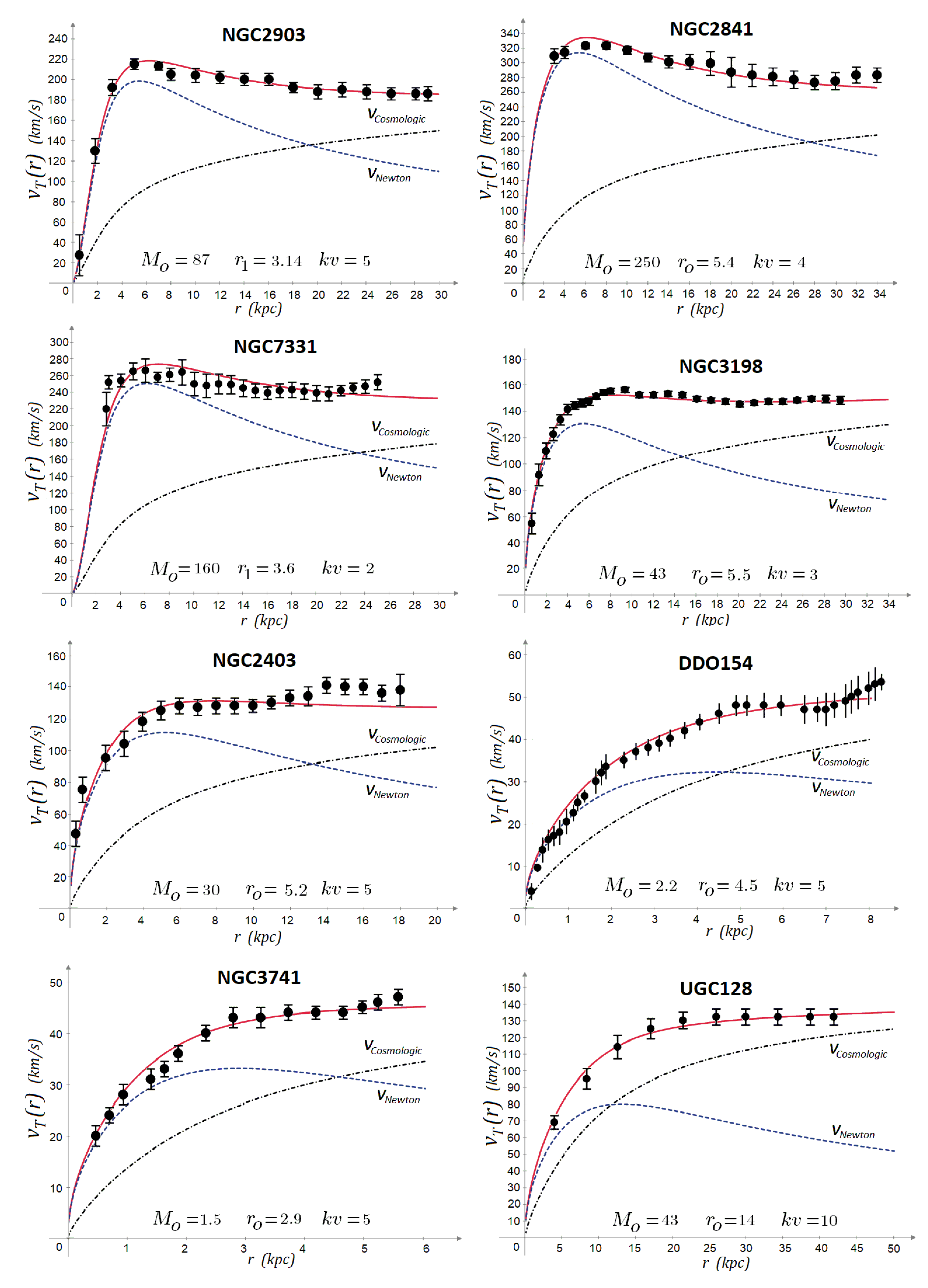
Now that we have equation (284), we can test its ability to reproduce observed galaxy rotation curves. Data from eight galaxies of varying sizes, masses, and rotation speeds were used to fit equation (284) by adjusting relevant parameters.

For each galaxy, we then fit the specific values of the galactic mass M₀ and the scale radius r₀ or r₁, depending on the chosen profile while the R_U and M_U parameters of the universe must be constant and with the values obtained before.

To conclude this section, the following figures present the rotation velocity curves of eight galaxies. The black dots (with error bars) represent the observed values from [13]. The blue dashed curves show the Newtonian velocity v_N(r), while the black dotted curves correspond to the cosmological velocity v_C(r). The red line is the total velocity v_t(r) obtained from equation (284). Galaxy masses M_o are given in units of 10⁹ M_⊙, and radial distances are expressed in kiloparsecs. From these plots, it can be concluded that equation (284) fits the observed rotation curves quite well. Therefore, the cosmological acceleration given by equation (248) provides a mechanism that can account for the shape of galactic rotation curves without explicitly invoking dark matter.

Figure 9. Rotation curves for different galaxies including cosmological velocity.

Figure 9. Rotation curves for different galaxies including cosmological velocity.

7.6. Wide Binary Systems

Wide binary systems are composed of two stars with masses on the order of one solar mass, whose dynamics are studied at distances of up to 200 astronomical units (au). The goal is to determine whether the relative acceleration between the stars follows the classical Newtonian behavior, or whether it agrees with the predictions of modified gravity theories such as MOND. This range of distances and masses has been chosen because it leads to accelerations on the order of the MOND characteristic constant, a₀ = 1.2×10⁻¹⁰ m/s².

It has been observed that, in this regime, wide binary systems exhibit dynamics consistent with Newtonian gravity and not with MOND 14. This is often interpreted as a significant challenge for MOND, which predicts deviations from Newtonian behavior in this weak-acceleration regime.

In this section, we apply the model proposed in this work, which introduces a cosmological acceleration projected onto 3D space, derived in previous sections. We analyze whether this additional term significantly affects the dynamics of these systems or, on the contrary, whether Newtonian behavior is preserved.

To do this, we compare the expressions for the Newtonian acceleration g_N(r) and the projected cosmological acceleration g_r(r), given by equations (259) and (248), respectively. Taking stellar masses on the order of 1 M_⊙, the associated vacuole radius is:

$$R_v=\sqrt[3]{{\displaystyle \frac{Mg}{M_U}}}\cdot R_U=3.17\cdot {10}^7\hspace{0.17em}au$$

(285)

This value is much larger than the distance range of interest (up to 200 au). In this regime, the Newtonian acceleration simplifies to:

$${\mathrm{g}}_{\mathrm{N}}\left(\mathrm{r}\right)=-{\displaystyle \frac{\mathrm{G}{\mathrm{M}}_{\mathrm{g}}}{{\mathrm{r}}^2}}\left(1-{\left({\displaystyle \frac{{\mathrm{k}}_{\mathrm{v}}\mathrm{r}}{{\mathrm{k}}_{\mathrm{v}}\mathrm{r}+{\mathrm{R}}_{\mathrm{v}}}}\right)}^2\right)\simeq -{\displaystyle \frac{\mathrm{G}{\mathrm{M}}_{\mathrm{g}}}{{\mathrm{r}}^2}}$$

(286)

Thus, the classical Newtonian form is recovered.

Regarding the cosmological acceleration, from equation (248), for r < < R_v, we can approximate:

$$g_r(r)={\displaystyle \frac{-G{M}_U}{R_U^2}}\sqrt{{\displaystyle \frac{R_s{R}_v}{r(k_{v}r+R_v)-R_s{R}_v}}}\simeq {\displaystyle \frac{-G{M}_U}{R_U^2}}\sqrt{{\displaystyle \frac{R_s{R}_v}{r(k_{v}r+R_v)}}}\simeq {\displaystyle \frac{-G{M}_U}{R_U^2}}\sqrt{{\displaystyle \frac{R_s}{r}}}$$

(287)

where R_s is the Schwarzschild radius of the system. Substituting the expression for R_s, we obtain:

$$g_r\left(r\right)\simeq {\displaystyle \frac{-G{M}_U}{R_U^2}}\sqrt{{\displaystyle \frac{2G{M}_g}{c^2\cdot r}}}$$

(288)

Now we can calculate the value of g_N(r) and g_r(r) for r = 200 au and we would have that:

$$g_N(200\mathrm{a}\mathrm{u})=1.48\cdot 10^{-7}{\mathrm{m}·\mathrm{s}}^{-2}>>g_r(200\mathrm{a}\mathrm{u})=5.01\cdot 10^{-13}{\mathrm{m}·\mathrm{s}}^{-2}$$

(289)

Therefore, the Newtonian acceleration term is several orders of magnitude larger than the cosmological acceleration.

By equating g_r(r) with g_N(r), we find the value of r at which both accelerations are equal:

$$\mathrm{r}=\sqrt[3]{{\displaystyle \frac{{\mathrm{M}}_{\mathrm{g}}\cdot {\mathrm{R}}_{\mathrm{U}}^4\cdot {\mathrm{c}}^2}{2\cdot \mathrm{G}\cdot {\mathrm{M}}_{\mathrm{U}}^2}}}\simeq 8.9\cdot {10}^5\hspace{0.17em}\mathrm{a}\mathrm{u}$$

(290)

This value is significantly greater than the typical 200 au scale of wide binary systems. Consequently, we conclude that within the range of distances considered, the dynamics of these systems remain purely Newtonian, in perfect agreement with observations. This prediction of the model sets it apart from MOND and reinforces its validity in low-acceleration regimes.

7.7. Velocity Dispersion in Galaxy Clusters: A 5D Virial-Like Relation Without Dark Matter

From equation (263), we have previously found that mass is proportional to the cube of velocity, that is, M ∝ v³. This leads us to postulate that the relationship between mass and the velocity dispersion σ_v in galaxy clusters should also follow the form:

$$M=A_{\sigma }\cdot {\sigma }_v^3$$

(291)

where A_σ is a proportionality constant.

This expression allows us, given a pair of values (M, σ_v), to determine A_σ, and using that value, check whether the observational data can be fitted accordingly. To this end, we use the following plot obtained from 15, which shows the velocity dispersion as a function of mass for different models such as MOND and Newton + dark matter (DM).

Figure 11. Predictions of velocity dispersion from several models.

Figure 11. Predictions of velocity dispersion from several models.

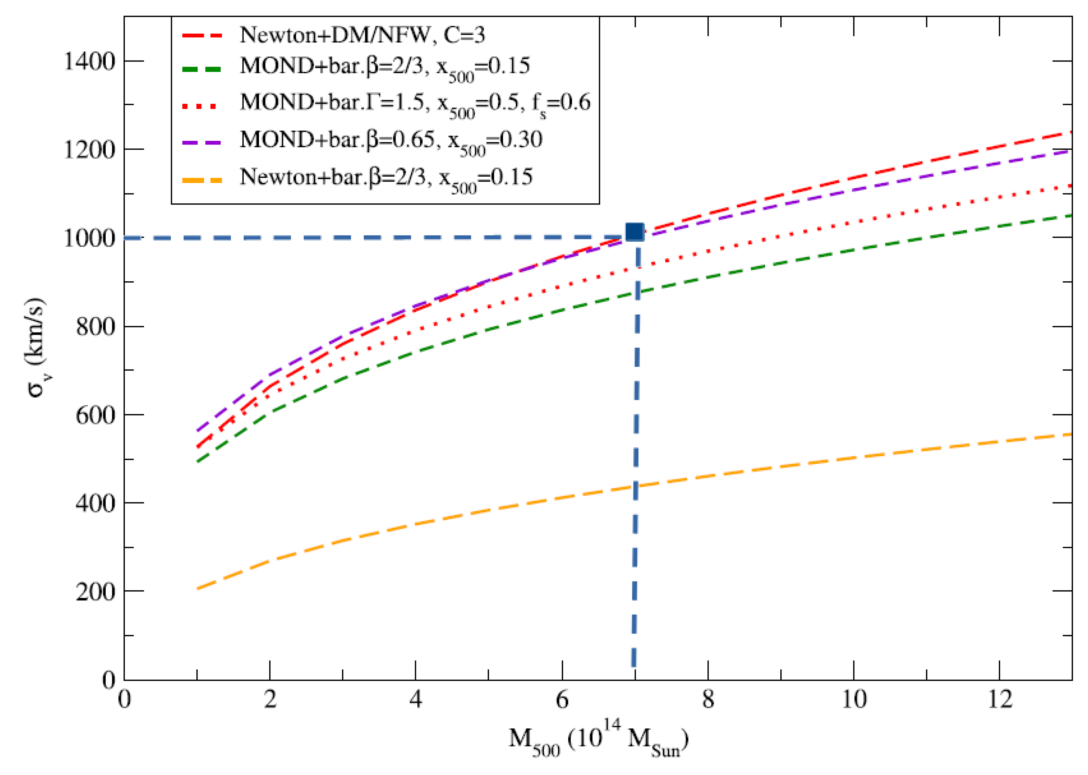
In the above figure, the masses along the X-axis, denoted M₅₀₀, are considered total masses in the Newton + DM case. For the MOND models, the baryonic mass is computed using the relation:

$$M_{bar.500}=0.117\cdot 10^{14}({\displaystyle \frac{M_{500}}{10^{14}{M}_{\odot }}}{)}^{1.16}{M}_{\odot }$$

(292)

In contrast with ΛCDM, where the dynamical mass includes dark matter, we assume that the relevant mass is the baryonic component, corresponding to 15% of the total mass

$$M_{bar.500}=0.15\cdot M_{500}\cdot {10}^{14}\cdot M_{\odot }$$

(293)

If we choose the point (7, 1000) in the graph, then the values used to calibrate A_σ become (0.15·7, 1000) = (1.05, 1000), which gives:

$$A_{\sigma }={\displaystyle \frac{M_{bar.500}}{{\sigma }^3}}={\displaystyle \frac{1.05\cdot {10}^{14}\cdot M_{\odot }}{{\left(1000km/s\right)}^3}}=105000{\displaystyle \frac{M_{\odot }}{{\left(km/s\right)}^3}}$$

(294)

Thus, the general expression for our model becomes:

$$M_{bar.500}=105000{\displaystyle \frac{M_{\odot }}{(km/s{)}^3}}\cdot {\sigma }_v^3$$

(295)

We now use this expression to test whether it correctly fits the data shown in the figure. The result is displayed in the following figure, where the blue squares represent predictions using equation (295) within the 5D model. As can be observed, the expression aligns very well with the red curve corresponding to the Newton + DM/NFW model.

Figure 12. Predictions of the velocity dispersions for the 5D model.

Figure 12. Predictions of the velocity dispersions for the 5D model.

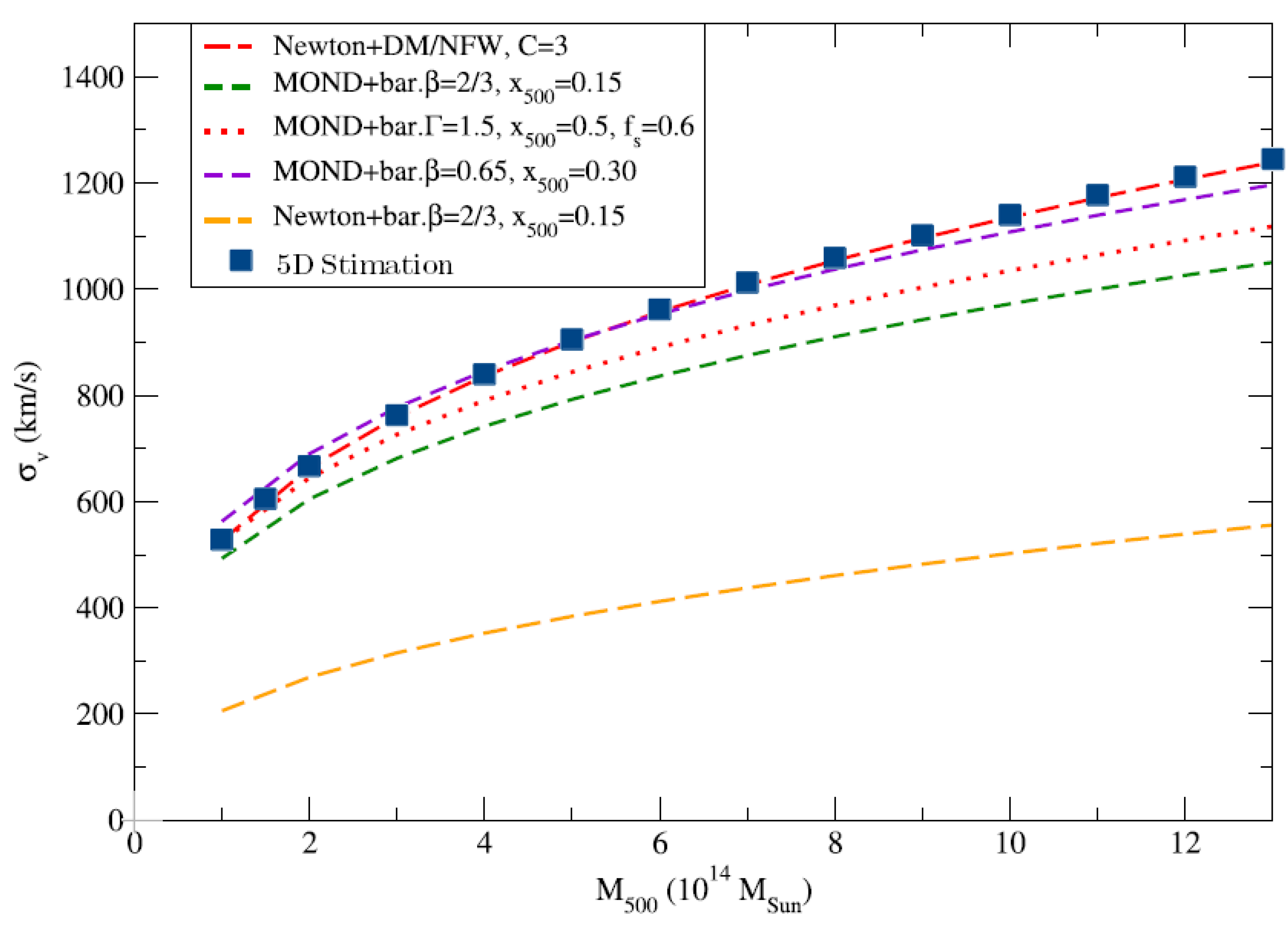
The final step is to check whether the value of A_σ, previously obtained by fitting, can be derived directly from the 5D velocity equation. To do this, we assume a proportional relationship between velocity and velocity dispersion of the form:

$$v=C\cdot {\sigma }_v$$

(296)

where v is the velocity given by equation (207). Therefore, the following must hold:

$$M_g\left(v\right)={\displaystyle \frac{c\cdot R_U^2}{G^2\cdot M_U}}\sqrt[4]{{\displaystyle \frac{R_U\cdot c^2\cdot k_v^3}{8\cdot G\cdot M_U}}}\cdot v^3={\displaystyle \frac{c\cdot R_U^2}{G^2\cdot M_U}}\sqrt[4]{{\displaystyle \frac{R_U\cdot c^2\cdot k_v^3}{8\cdot G\cdot M_U}}}\cdot {\left(C\cdot {\sigma }_v\right)}^3$$

(297)

Comparing with equation (291), we obtain:

$${\displaystyle \frac{c\cdot R_U^2}{G^2\cdot M_U}}\sqrt[4]{{\displaystyle \frac{R_U\cdot c^2\cdot k_v^3}{8\cdot G\cdot M_U}}}\cdot C^3=A_{\sigma }=105000{\displaystyle \frac{M_{\odot }}{\mathrm{k}{\mathrm{m}}^3/{\mathrm{s}}^3}}$$

(298)

Using k_v = 5 (similar to the value used in the study of galaxy rotation curves), and substituting all known values, we find:

$$v=2.44\cdot {\sigma }_v$$

(299)

While it is usually considered that for self-gravitating systems:

$$v=\sqrt{3}\cdot {\sigma }_v\simeq 1.73\cdot {\sigma }_v$$

(300)

obtaining the correct value of A_σ in equation (298) by simply taking C = 2.44 can be regarded as a success of the 5D model, demonstrating a precise match between the theoretical framework and the empirical fit.

We can therefore conclude that the 5D geometrical model presented in this work, through its M ∝ v³ relation, is capable of explaining velocity dispersion in galaxy clusters using only the baryonic mass, without requiring the presence of dark matter.

8. Conclusions

The Standard Model of Cosmology, ΛCDM, while remarkably successful in fitting a vast range of observational data, rests upon an increasingly complex and fragmented theoretical foundation. It requires the postulation of three separate and physically unmotivated pillars to match reality: an inflationary epoch driven by an unknown scalar field, a mysterious cold dark matter particle that has eluded all direct detection, and a perplexing dark energy component whose nature remains a profound enigma.

This work proposes a geometric alternative to inflation, dark matter, and dark energy by attributing these phenomena to a geometric framework in 5D, though further validation through numerical simulations and observational tests is required to confirm its viability

From this purely geometric foundation, a complete and self-consistent cosmology emerges. We have shown that:

• Our framework offers an alternative to inflation by postulating a fundamental link between curvature and inhomogeneity (|Ω_k| = 1/2 δ_ρ), motivated by the physics of structure formation, and using absolute simultaneity derived from the privileged framework reference, the flatness and horizon problems are resolved intrinsically. This framework, calibrated with the observed anisotropies of the CMB, correctly predicts the observed angular scales of the CMB and BAO, with deviations of approximately 7% and 2.3%, a feat achieved without any inflationary mechanism.
• The phenomena attributed to dark matter may emerge naturally from the geometric projection of cosmological acceleration in our 5D model. The global deceleration of the 5D hypersphere projects a real, calculable acceleration (g_C) onto our 3D space. This single mechanism has been shown to reproduce the dynamics of galaxies across all scales — from massive spirals like NGC 2841 to gas-dominated dwarfs like NGC 3741 — without the need for dark matter halos. This framework not only explains flat rotation curves but also derives a Tully-Fisher-like relation (M ∝ v³) and is consistent with the velocity dispersions in galaxy clusters and the dynamics of wide binary systems.
• MOND emerges as a derived consequence, not a fundamental law. The phenomenological success of Modified Newtonian Dynamics is explained within our model. The MOND acceleration scale a₀ is not a new constant of nature, but an emergent quantity derived from the fundamental parameters of the universe (M_U, R₀), thereby providing a theoretical foundation for Milgrom's empirical law.
• This model proposes that the apparent dimming of Type Ia supernovae arises from an intrinsic luminosity–redshift dependence, L(z)∝(1+z)⁻¹, rather than from accelerated expansion. This luminosity evolution eliminates the need for dark energy and leads to a consistent reinterpretation of the supernova Hubble diagram. When combined with the geometric framework of the 5D hyperspherical universe, the model successfully reproduces the observed angular scales of the CMB and BAO without introducing additional free parameters.
• This model raises questions about the global applicability of the Special Relativity to the universe, suggesting the need for a generalized kinematic framework, as explored in [16], though further theoretical development is necessary.

The internal consistency of this model is its greatest strength. The fundamental parameters of the universe (M_U, M_R and R₀), derived from the physics of the Cosmic Microwave Background, are precisely those required to explain the dynamics of galaxies billions of years later. Three independent observational regimes — the primordial universe, the dynamics of galaxies, and the phenomenology of MOND — all converge on the same set of universal constants.

Unlike ΛCDM, which relies on multiple components to explain observations, this model seeks a unified description based on 5D geometry, aiming for simplicity while acknowledging the need for rigorous testing against observational data. It suggests that the universe is not filled with mysterious substances, but that its deepest secrets are written in the language of pure geometry. We present this model not as a final theory, but as a compelling and falsifiable alternative, inviting the scientific community to explore its predictions and confront the beautiful, simple, and purely geometric universe it describes.

Table 4. Present-day values of the 3-Sphere universe parameters.

Symbol	Description	Estimated Value	Units
H0	Hubble parameter (today)	48.7	Km/s/Mpc
MU	Total mass of the universe	1.24 x 1060	kg
R0	Radius of the hypersphere (today)	4.05 × 1028	m
MR	Equivalent mass of radiation	4.32 × 1051	kg
Rs	Maximum Radius of the hypersphere	1.841 × 1033	m
RR	Radiation Radius	6.421 x 1024	m
Ωk0	Curvature parameter	2.2 x 10-5	-
ρR	Density of radiation of the universe (today)	7.060 x 10-31	kg/m3
τ0	Proper time (comoving observer)	13.39 × 109	years
t0	Coordinate time (today)	4.28 × 1012	years
τRM	Transition from radiation to matter domination proper time	15.7x 103	years
τCMB	CMB recombination time	3.12 x 105	years
θs	Angular size of the sound horizon at decoupling	0.555	degrees
rs	Comovil distance of CMB	115.3	Mpc
θBAO	Angular Scale of BAO	4.18	degrees
gc(τ0)	Cosmological acceleration (today)	5.04 x 10-8	m/s²
CMV	Constant of proportionality between mass and velocity3 (Eq.(265))	7.25x103	M⊙/km3s3
Aσ	Constant of proportionality between mass and velocity dispersion (Eq. (294))	105000	M⊙/km3s3

Table 4. Present-day values of the 3-Sphere universe parameters.

Symbol	Description	Estimated Value	Units
H0	Hubble parameter (today)	48.7	Km/s/Mpc
MU	Total mass of the universe	1.24 x 1060	kg
R0	Radius of the hypersphere (today)	4.05 × 1028	m
MR	Equivalent mass of radiation	4.32 × 1051	kg
Rs	Maximum Radius of the hypersphere	1.841 × 1033	m
RR	Radiation Radius	6.421 x 1024	m
Ωk0	Curvature parameter	2.2 x 10-5	-
ρR	Density of radiation of the universe (today)	7.060 x 10-31	kg/m3
τ0	Proper time (comoving observer)	13.39 × 109	years
t0	Coordinate time (today)	4.28 × 1012	years
τRM	Transition from radiation to matter domination proper time	15.7x 103	years
τCMB	CMB recombination time	3.12 x 105	years
θs	Angular size of the sound horizon at decoupling	0.555	degrees
rs	Comovil distance of CMB	115.3	Mpc
θBAO	Angular Scale of BAO	4.18	degrees
gc(τ0)	Cosmological acceleration (today)	5.04 x 10-8	m/s²
CMV	Constant of proportionality between mass and velocity3 (Eq.(265))	7.25x103	M⊙/km3s3
Aσ	Constant of proportionality between mass and velocity dispersion (Eq. (294))	105000	M⊙/km3s3

To conclude this section, we leave a table with the summary of all the parameters and their values of this 3-Sphere universe.

9. Discussions

The 3-Sphere Model, as presented in this work, offers a self-consistent and purely geometric framework that unifies a wide range of cosmological and astrophysical phenomena. However, its departure from the standard ΛCDM paradigm is profound, leading to a series of unique and eminently falsifiable predictions. The ultimate test of this theory will not be its internal elegance, but its ability to withstand rigorous observational scrutiny. We outline below the key experimental tests that could either corroborate or refute this model.

Falsifiable Predictions of the 3-Sphere Model:

a)

The Cosmic Microwave Background: While our analytical calculations predict the angular scale of the first acoustic peak with remarkable accuracy (~7%), this represents only a fraction of the information encoded in the CMB. A complete numerical evolution of the coupled Boltzmann equations within our cosmological background is the most crucial next step. This model predicts a specific history of perturbation growth (e.g., δ_ρ ∝ R² in the radiation era) and a unique relationship between density and temperature fluctuations (δ_ρ ≈ 4 δ_T). These will inevitably lead to subtle but detectable deviations from the ΛCDM predictions for the higher acoustic peaks and the polarization spectrum. A disagreement with the precision data from Planck in these areas would constitute a strong falsification.

b)

The Baryonic Tully-Fisher Relation: Unlike the empirical L ∝ v⁴ relation, our model fundamentally predicts that baryonic mass scales with the cube of the flat rotation velocity, M_b ∝ v³. While current data can be fitted by both relations within their scatter, future large-scale surveys of galactic dynamics (e.g., with the Square Kilometre Array) could distinguish between a v³ and a v⁴ scaling with high statistical significance, providing a definitive test.

c)

Galaxy Rotation Curves at Large Radii: A key feature of our model is the modification of the local metric to ensure a smooth embedding within the global hypersphere. This predicts that the flat rotation curves of galaxies should persist out to enormous distances, potentially up to 1-2 Megaparsecs, before any decline is observed. Although there are already some measurements such as 9 that seem to confirm this prediction of the model, a greater number of measurements in this regard would be necessary.

d)

The Dynamics of Wide Binary Stars and Galaxy Clusters: The model makes distinct predictions at opposite ends of the scale spectrum. It successfully reproduces the dynamics of galaxy clusters, but also predicts a purely Newtonian regime for the very low accelerations found in wide binary star systems, in agreement with recent observations. Any confirmed, statistically significant deviation from Newtonian gravity in wide binaries would pose a serious problem for this theory, distinguishing it from MOND-like paradigms.

10. Conceptual and Philosophical Implications

Beyond these direct tests, our framework invites a profound re-evaluation of several foundational concepts in cosmology:

• The Impossibility of a Flat Universe: Our fundamental law, |Ω_k| = 1/2 δ_ρ, implies that a perfectly homogeneous universe (δ_ρ = 0) must be perfectly flat (Ω_k = 0), and vice versa. However, the Uncertainty Principle guarantees the existence of primordial quantum fluctuations. Therefore, a perfectly homogeneous universe cannot exist. It follows that a truly flat universe is a physical impossibility. The "near-flatness" we observe is not an approach to k = 0, but a measure of the extraordinary initial homogeneity of our intrinsically curved (k=+1) cosmos.
• A Black Hole Universe: The maximum radius of our closed universe, R_S, is not just a parameter, but is shown to be equivalent to the Schwarzschild radius corresponding to its total mass-energy content, M_U. This suggests a startling possibility: our entire 3-sphere universe may be the interior of a five-dimensional black hole. The expansion and eventual contraction we experience would be the motion of our 3-brane from the singularity towards the event horizon and back again.
• A Window into Quantum Gravity: The cornerstone of our alternative to inflation is the proposed law connecting global curvature to local inhomogeneity, |Ω_k| = 1/2 δ_ρ. We have justified this relation through the physics of structure formation, but its fundamental origin may be much deeper. This law suggests a profound link between the macroscopic geometry of spacetime (Ω_k) and the statistical properties of its quantum fluctuations (δ_ρ). It provides a concrete, phenomenological equation that any candidate theory of quantum gravity must be able to reproduce. The universe, in this view, becomes the ultimate laboratory for probing the interface between General Relativity and quantum mechanics, where the "grittiness" of quantum spacetime itself dictates the large-scale curvature of the cosmos.

11. Future Work

This paper lays the groundwork for a rich program of theoretical and phenomenological research. The most urgent priorities are:

• A Full Theory of Perturbations: To move beyond analytical estimates and rigorously test the model against the full CMB power spectrum and polarization data. This would involve deriving and numerically solving the modified Boltzmann equations to predict the Cl spectrum, including the calculation of the δ_ρ - δ_T relation from first principles.
• The Nature of the Curvature-Inhomogeneity Law: To explore if the postulated law |Ω_k| = 1/2 δ_ρ can be derived from a more fundamental theory, possibly from the principles of quantum gravity applied to a 5D spacetime.
• Gravitational Lensing Analysis: A critical next step is the study of light deflection within the modified Schwarzschild-like metric (Eq. (255)). It is essential to verify if the projected cosmological acceleration (g_C) and the geometric screening function f(r) correctly account for gravitational lensing observations. Specifically, the model must demonstrate that it can reproduce the observed mass profiles in strong and weak lensing (such as in galaxy clusters and cosmic shear) without the inclusion of dark matter, ensuring that null geodesics are affected by the 5D geometric projection in a manner consistent with astrophysical data.
• Large-Scale Structure and N-body Simulations: To compete with the ΛCDM paradigm, the model requires testing through numerical N-body simulations. By incorporating the projected acceleration term (g_C) and the continuity-driven screening f(r), we aim to investigate the formation of the "cosmic web" and the growth of large-scale structures. This will determine if a purely geometric, decelerating universe can provide the necessary stability and clustering timescales to match the observed distribution of galaxies and voids.
• Physical Drivers of Luminosity Evolution: The hypothesis L(z)∝(1+z)⁻¹ currently serves as a necessary condition to reconcile a decelerating universe with supernova observations. Future research should focus on providing a robust physical basis for this evolution. This includes analyzing the effects of progenitor metallicity and stellar population ages at high redshift, as well as exploring whether the extrinsic kinematic time dilation (dτ) between the bulk and the brane induces variations in effective physical rates or emission processes that manifest as the observed luminosity decay.
• The Evolution of the Contracting Universe: A notable implication of the law |Ω_k| ∝ δ_ρ is the behavior of the universe during a potential contraction phase (R(t) decreasing). Since |Ω_k| scales with R(t) in a matter-dominated era, the model predicts a forced return to homogeneity ( δ_ρ→0 ) as the hypersphere contracts. Preliminary analysis of the geodesic equations (Eq. (227)) suggests that the projected acceleration g_C may undergo a sign change when Ṙ < 0, potentially generating a large-scale repulsive effect. Future work will focus on determining if this mechanism provides a geometric basis for a "Big Bounce" scenario, preventing a final singularity and ensuring a smooth transition into a new cycle.

In summary, this model, while radical, offers a path towards a more unified and geometric understanding of the cosmos. Each of these future steps will serve to either solidify its foundations or reveal its limitations, as is the true spirit of scientific inquiry.

12. Relation with Previous Works

This paper constitutes a substantially revised and extended version of Error! Reference source not found..

References

- Knop, R. A.; et al. New Constraints on ΩM, ΩΛ, and w from an Independent Set of 11 High-Redshift Supernovae Observed with the Hubble Space Telescope. The Astrophysical Journal 2003, Volume 598(Issue 1), 102–137. [CrossRef]
- Chung, C.; et al. “Strong progenitor age bias in supernova cosmology – I. Robust and ubiquitous evidence from a larger sample of host galaxies in a broader redshift range”. Monthly Notices of the Royal Astronomical Society 2025, Volume 538(Issue 4, April 2025), Pages 3340–3350. [CrossRef]
- J. Son et al. “Strong progenitor age bias in supernova cosmology – II. Alignment with DESI BAO and signs of a non-accelerating universe”. Monthly Notices of the Royal Astronomical Society 2025, Volume 544(Issue 1, November 2025), Pages 975–987. [CrossRef]
- Alan H. Guth. Inflationary universe: A possible solution to the horizon and flatness problems. Phys. Rev. D 1981, 23, 347. [CrossRef]
- Mather, J. C.; Fixsen, D. J.; Shafer, R. A.; Mosier, C.; Wilkinson, D. T. Calibrator Design for the Far-Infrared Absolute Spectrophotometer (FIRAS). The Astrophysical Journal 1999, 512(2), 511–520. [Google Scholar] [CrossRef]
- Buchert, T. On Average Properties of Inhomogeneous Fluids in General Relativity: Dust Cosmologies. General Relativity and Gravitation 2000, 32, 105–125. [Google Scholar] [CrossRef]
- Planck Collaboration. Planck 2018 results. VII. Isotropy and Statistics of the CMB. In Astronomy & Astrophysics; 2020; Volume 641, p. A7. [Google Scholar] [CrossRef]
- Tully, R. B.; Fisher, J. R. A New Method of Determining Distances to Galaxies. Astronomy and Astrophysics 1977, 54(3), 661–673. [Google Scholar]
- Tobias Mistele et al “Indefinitely Flat Circular Velocities and the Baryonic Tully–Fisher Relation from Weak Lensing”. The Astrophysical Journal Letters 2024, Volume 969, Number1. [CrossRef]
- Einstein, A.; Straus, E. G. The influence of the expansion of space on the gravitation fields surrounding the individual stars. Reviews of Modern Physics 1945, 17(2–3), 120–124. [Google Scholar] [CrossRef]
- Milgrom, M. A modification of the Newtonian dynamics as a possible alternative to the hidden mass hypothesis. Astrophysical Journal 1983, 270, 365–370. [Google Scholar] [CrossRef]
- Lelli, F.; McGaugh, S. S.; Schombert, J. M. The SPARC data base: 174 galaxy rotation curves and their dark baryonic decomposition. The Astronomical Journal 2016, 152(6), 157. [Google Scholar] [CrossRef]
- Marr, John. Galaxy rotation curves with log-normal density distribution. In Monthly Notices of the Royal Astronomical Society; 2015; p. 448. [CrossRef]
- Pittordis, C.; Sutherland, W. Wide binaries as a critical test of classical gravity: confronting Gaia DR3 with MOND predictions. Monthly Notices of the Royal Astronomical Society 2023, 519, 3937–3956. [Google Scholar]
- López-Corredoira, M; Betancort-Rijo, J E; Scarpa, R; Chrobáková, Ž. Virial theorem in clusters of galaxies with MOND. Monthly Notices of the Royal Astronomical Society 2022, Volume 517(Issue 4, December 2022), 5734–5743. [Google Scholar] [CrossRef]
- José Gabriel Ramírez Escalona. (2024). Is the Special Relativity Compatible With Einstein’s Static Universe?Proposal for New “Generic” Transformations. The Twin Paradox. Qeios. [CrossRef]
- Ramírez Escalona, J. G. A Unified Cosmology in a 5D Hypersphere: A Geometric Framework Without Inflation, Dark Matter, or Dark Energy. Preprints 2025, 2025101475. [CrossRef]
Disclaimer/Publisher’s Note: The statements, opinions and data contained in all publications are solely those of the individual author(s) and contributor(s) and not of MDPI and/or the editor(s). MDPI and/or the editor(s) disclaim responsibility for any injury to people or property resulting from any ideas, methods, instructions or products referred to in the content. |
© 2026 by the author. Licensee MDPI, Basel, Switzerland. This article is an open access article distributed under the terms and conditions of the Creative Commons Attribution (CC BY) license.
Copyright: This open access article is published under a Creative Commons CC BY 4.0 license, which permit the free download, distribution, and reuse, provided that the author and preprint are cited in any reuse.