Submitted:
20 November 2024
Posted:
21 November 2024
You are already at the latest version
Abstract
Today's Lambda Cold Dark Mater (ΛCMD) cosmology model is in crisis and requires a new Kuhn paradigm. This new paradigm is presented here, analogous to shift from geocentric to a heliocentric system. All our cosmological measurements are measurements INSIDE (IN) the universe, not OUTSIDE (OUT) of space-time. This is not a trivial observation, because (IN) measurements gives a distorted picture of a simpler, true (OUT) cosmology. ΛCDM cosmology is a distorted internal view of the (OUT) spherical, linearly expanding universe using Brans-Dicke's theory generalization: Self Creating Cosmology (SCC). This (OUT) SCC model reproduces (IN) ΛCDM cosmology parameters: the ratio of matter to dark energy, the equation of the dark energy state, the time of dark energy dominance, and the value of today's acceleration. In SCC cosmology model Ωk = (-1/12), but like some cosmic “mimicry” a spherical universe “pretends” to be flat from INSIDE view. The predicted theoretical ratio of radial to transverse distance is 1.0847 for z = 1089.8, compared to experimental ratio H0(SNe)/H0(CMB) = 1.0858 ± 0.0127. This same ratio solves the S8 tension. The unexpectedly early appearance of various structures detected by JWST for large redshift is caused by incorrectly determined relation of t(z).
Keywords:
cosmology crisis
; Hubble tension
; S8 tension
; Self Creating Cosmology
; JWST high z measurements
1. Introduction
Kuhn [1] changed the classical understanding of the gradual evolution of science into a sequence of leapfrog scientific revolutions, where a new paradigm based on new principles is established. As an example, he gives the Copernican revolution and the jump from the Geocentric to the Heliocentric description of the Solar System. New paradigms solve generally recognized problems while preserving the ability to solve problems through previous paradigms.
In particle physics, due to the statistical nature of the measurements, the minimum limit for accepting new discoveries is a signal for which the probability to be only a statistical fluctuation is at the level of 5 σ. The value of the cosmological important Hubble constant H0 measured directly by type Ia supernovae (SNe) or determined from the Cosmic Microwave Background radiation spectrum (CMB) by the Lambda Cold Dark Mater (ΛCDM) cosmological model gives different values. This deviation is now at the level of 5 σ so this should also be accepted as a fact.
One way to solve this problem is to introduce another new parameter into the ΛCDM model, for example, by changing the amount ωDM = -1 from the dark energy state equation, so that ΛCDM would become the ωΛCDM model. This is like inserting new circles within circles into a Geocentric model. There are other problems besides this so-called Hubble tension: S8 tension, the problem of primordial lithium (Li7/H ratio), unexpected new measurement results by the James Webb Space Telescope (JWST). It is time for a new paradigm in cosmology.
Kuhn's paradigm shift requires the “sacrifice” of some “obvious” and “common-sense” but wrong unconscious understanding that is implicitly implied until it is realized that it is wrong and is replaced with another principle, sometimes difficult to accept. For example, the “obvious fact” of the Earth's quiescence is replaced by its rotation on its axis and around the Sun while “sacrificing” the idea that the Earth is at the center of the universe. There is an almost perfect mathematical “isomorphism” between “mappings”:
New Perspective: Geocentric Model → Heliocentric Model and:
A new perspective: ΛCDM cosmology → a 3D-spherical universe that spreads uniformly.
All the great truths later become almost banal, and that is why they are difficult to reach, as the conclusion of the fish that it is in the water. Figure 1 is a popular representation of the universe from the Big Bang (BB) to the present day, according to ΛCDM cosmology. There is something unusual about that picture. Without going into the question of the existence of the Creator, Figure 1 is a representation of the universe from God's perspective because, by definition, God is OUTSIDE (OUT) of space and time, and we are INSIDE (IN) space and time, and all our measurements are INSIDE the universe. Do (IN)-measurements give an accurate (OUT)-cosmology? The mentioned “isomorphism” indicates that it does not.
Just as the constant light speed principle is sufficient for the development of the Special Theory of Relativity (STR), so the distinction between (IN) and (OUT) cosmological quantities is sufficient to reproduce the (ω)ΛCDM model from a simple (OUT) model of a uniformly expanding 3D-spherical universe. For the cosmological expansion of the universe beyond the Hubble radius, the following argument is used:
In Einstein's STR, velocities greater than c = 299,792,458 m/s are not possible, but they are possible in GTR because it is not the motion of the body but the expansion of the space itself. For simplicity, I use dimensionless quantities in this work (time t = 0 for BB, t = 1 now, scale a(t) = t, Hubble constant H0 = 1, Hubble radius DH = 1, speed of light c = 1). Next to the cosmological parameters, if necessary, I add (IN) or (OUT). All dependencies of all quantities (INside and OUTside) as time functions, arise from the identity equation a(t) = t and can be easily reproduced using some Graphing Calculator (for example Desmos).
2. Model Development
2.1. (IN) and (OUT) recessionary velocity
Here are two thought experiments (Earth, A, and B are on the same line):
- Let at R = 0.5 galaxy A move away from us at a speed of 0.5 c, and at a distance R = 1, galaxy B moves away from galaxy A at a speed of 0.5 c. Then in GTR galaxy B is moving away from us at a speed of 0.5 c + 0.5 c = c .
- Let rocket A move away from us at a speed of 0.5 c, and rocket B moves away from rocket A at a speed of 0.5 c. Then rocket B moves away from us at a speed of 0.8 c, because in STR the relativistic addition of velocities applies (for c = 1):
The differences in the summing of velocities in 1 and 2 are because (implicitly) GTR and cosmology are defined from the (OUT) perspective and STR from the (IN) perspective. The collateral victim of this distinction is the so-called Warp drive, the idea of traveling faster than light in a space-time “bubble” in which the rocket is stationary. Equidistant galaxies on the line with R(Milky-Way) = R(0) = 0 are (now) moving away according to Hubble's law at an (OUT) velocity v(R) = H0∙R = R , and their (IN) velocity is v(R) = tanh(R), which is always less than c=1 and less than (OUT) R = v(R). For this (OUT) a(t) = t model radial (OUT) comoving distance is
so, (IN) velocity is v(R(t)) = tanh(-ln(t)) = (1-t2)/(1+t2) and (OUT) v(t) = -ln(t). There are as many as three different definitions of redshift z: Doppler, cosmological and gravitational. For (IN) v(t) from the expression for Doppler redshift, we get:
Thus, the relativistic Doppler redshift for the (IN) recessionary velocity of the galaxy due to the expansion of the universe is equal to the cosmological redshift due to the change in the scale a(t). This is the same cosmological redshift seen from (IN) and (OUT) perspective (Doppler and cosmological).
2.2. (IN) and (OUT) radial comoving distance
Figure 2 shows a schematized representation of the dependence of the (OUT) radial comoving distance of (OUT) R(t) for symbolical one-year cosmological (IN) measurement. The space-time “stairs” for the 3 different distances is shown, for the central one enlarged, corresponding to HERE and NOW “stair” of 1 light year / 1 year. From similar triangles and using the relativistic contraction of the “stairs” by 1/γ factor, it is easy to obtain that the infinitesimal (IN) length of the “stairs” is:
with
It is also
so:
Thus, (IN) dR(t) can be understood in two complementary ways: either as the product of the (now) time interval dt and the scaled sum of the speed of light and the recessional (OUT) velocity (1+v)/t, contracted via the gamma factor for the (IN) velocity γ, or as the product of the (past) time interval dt’ and the sum of the light and (IN) velocity (1+v). The (IN) radial comoving distance is
With the substitution r = -ln(t), the (IN) radial distance R(t) expressed over the (OUT) radial distance r(t) is obtained:
3. Results
3.1. The (OUT) SCC cosmology reproduces (IN) ΛCMD cosmology
Analogous to the problem of deformation in cartographic projections from a curved to a flat surface (or vice versa), there is a similar problem of "projection" of the universe from the OUT perspective to the IN perspective. Thus, it is possible to "deform" the OUT into the IN perspective in several different ways. For example, in a "projection" used here time is equal in the IN and OUT perspectives. This leads to a slightly nonlinear function a(t) = t + ε(t) where the function ε(t) takes on small values. A "projection" is possible in which the OUT scale is equal to the IN scale "a" where t(a) = a + δ(a). Again, the function δ(t) takes small values. It is also possible to express the IN scale and time parametrically, of the form a(x) and t(x), a slightly nonlinear functions of the parameter x.
The (IN) radial distance R(r) (Eq. 9) is finite even for the infinite (OUT) distance (r) and is equal to 3.4027. According to the ΛCDM model, the observable universe has an age of 13.77 Gy and a radius of 46.6 Gly, giving a ratio of 3.3842. This is only 0.54% less than the 3.4027 obtained from (OUT) a(t) = t, within the limits of measurement precision, which is the first, extremely accurate confirmation of this new paradigm.
From Hubble's law (for any epoch) H(t) = v(R(t))/R(t), and a(t) = t it follows that v(R) = const = (OUT)R, where the radial comoving distance (OUT) R is constant for a given galaxy, but due to the expansion is v(R(t)) = R(t)/t = -ln(t)/t and (OUT) R(t) = -ln(t) so, (OUT) H(t) = v(R(t))/(OUT)R(t) = 1/t. On the other hand, (IN) H(t) = (-ln(t)/t)/((IN)R(t)). (IN) R(t) is defined by Eq. (8). The reciprocal of 1/(OUT)H(t) is equal to the Hubble radius DH(t) = t = (OUT)T(t). The reciprocal of (IN) H(t) is a slightly nonlinear function (IN) T(t). The deceleration parameter q(t) is defined as
where obviously (OUT) q(t) = const = 0. However, due to the (apparent) nonlinearity of (IN) T(t), it is obtained that for t > 0.5523 the (IN) q(t) becomes negative, i.e. the universe expansion apparently accelerates and for t = 1 (IN) q0(t=1) is exactly -1/2. This is another confirmation of this paradigm since, according to the ΛCMD model, q0= -0.55. The (IN) q(t) becomes negative for t = 0.5523 for any epoch of the universe and has a value of -1/2 at the end of each epoch, since this is the apparent effect (such as a rainbow or a mirage) because of (IN)-measurements. From the apparent (IN) H(t) scale (IN) a(t) is determined as follows:
The scale (IN) a(t) is slightly nonlinear too. Figure 3 shows the (apparent) (IN) a(t) and (IN) T(t) which are (OUT)-identity functions (a(t) = t and T(t) = t). For t = 0.5523, when (IN) q(t) becomes negative, is (IN) a(t) = 0.5886 (according to Planck data [2] this occurs when a is about 0.6).
According to the ΛCMD model, when the expansion of the universe changes from deceleration to acceleration scale a is equal to (ΩM/2ΩDE)1/3, q0 = (ΩM+(1+3ωDE)ΩDE)/2. So, with the condition ΩM + ΩDE = 1 by including a = 0.5886 and q0 = -1/2 the solutions of these three equations are:
ΩM = 0.2897, ΩDE = 0.7103 and ωDE = -0.9386, for ωΛCMD model
With fixed ω = -1, q0 = -1/2, and the conditions ΩM + ΩDE = 1, the solutions are
ΩM = 1/3 = 0.3333, ΩDE = 2/3 = 0.6667, and a = 4-1/3 = 0.6300 for ΛCMD model
The data from the analysis of CMB radiation [2] are
which are roughly somewhere between the two (IN) solutions. This match, paradoxically, confirms that ΛCMD or here extended ωΛCMD is a distorted (IN)-image of a 3D-spherical universe with scale a(t) = t. So, ΩM, ΩDE (and added ωDE) should be understood only as the parameters by which this distorted image fits.
ΩM = 0.315 ± 0.007, ΩDE = 0.6847 ± 0.0073 (with the assumed ωDE= -1),
According to the ΛCDM model, it is
It is possible to find ΩM via (IN) T(t) and (IN) a(t) so that δ(t) is minimal:
Figure 4 shows the difference (T(t) - T’(t)) for the minimum values δ(0) (blue) and δ(0.4) (red). For t = 0, the minimum δ(0) = 0.00584, which is extremely small, considering that the calculation of apparent (IN) a(t) and (IN) T(t) has nothing to do with the ΛCDM model. This minimum δ(0) is achieved for
ΩM = 0.3041 and ΩDE = 0.6959.
For t = 0.4 (corresponding to the measurement limit of Type Ia supernovae (SNe) to z < 1.4 [3]) the minimum is δ(0.4) = 0.00282, for
ΩM = 0.3104 and ΩDE = 0.6896.
For the distance of the angular diameter, which is determined by measuring the angle at which an object of known size can be seen, the following applies:
so, the maximum angular diameter distance for a(t) = 1/e where e = 2.71828 is Euler's constant, which corresponds to the redshift zmax = 1.71828. This is another example of the perfect cosmological principle that the universe is always and everywhere homogeneous, isotropic and stationary in time, has the same (OUT) (due to linearity) and apparent (IN) characteristics in every epoch.
There are many authors ([4], and the literature attached there), starting with Milne [5], who use some variant of the linear model a(t) = t. Thus, Melia and Yennapureddy [6], who using a sample of 140 quasar nuclei obtained zmax = 1.70 ± 0.20 and conclude that the linear model of the expansion of the universe has the highest (92.8 %) probability of being correct, greater than the ΛCDM model.
3.2. The "weakest link" of this model
The CMB spectrum confirms that we live in a flat universe, which is problematic for all models of a linearly growing universe, because for z = 1089.8, the (OUT) radial comoving distance is R = 6.9947, and it should be RΛCDM = 3.3140. Although (IN) R= 3.3862 is only 2.2 % larger than RΛCDM, this does not detract from the problem, since for a flat universe the transverse distance remains D = 6.9947. The only solution, which is also the weakest “link in the chain” of this new paradigm, is that we live in a 3-sphere universe with these three unlikely coincidences:
- The universe is (OUT) spherically curved that at a certain z the radial (IN) R and the transverse (IN) D comoving distance are equal.
- This z must correspond to the time of CMB formation (recombination).
- The GTR should be modified to contain the (OUT) cosmological solution a(t) = t with Ωk which satisfies conditions 1 and 2.
Such coincidences are not unknown to the history of science (for example, Hoyle's resonance state C12, the opacity of water, the apparent size of the Moon and the Sun from Earth). For z = 1089.8 (OUT) comoving distance is R = 6.9947, (IN) comoving distance is R = 3.3862, so (IN) transverse comoving distance must be D = 3.3862 to make the (IN) universe look flat for CMB spectrum. This gives the condition
The numerical solution of this nonlinear equation gives Ωk = (-1/13.1048) ≈ (-1/13). There are many alternatives to GTR offered, but I have narrowed my search down to those theories that contain GTR as a special case, that is, Brans-Dicke (BD) theories of gravity. Kofinas [7] identifies only three possible types of “natural” generalizations of BD theories in which the stress-energy tensor is not conserved. One of these theories of the second type is Barber's model of cosmology [8, 9, 10] which Barber calls Self Creation Cosmology (SCC), for which the cosmological solution is a(t) = t and Ωk = (-1/12).
3.3. becomes the crowning proof of (OUT) SCC cosmology
Like the story of the Dirac equation, the biggest problem with this (OUT) a(t) = t model, thanks to Barber's SCC model, becomes its greatest triumph. Because 13.1048 is NOT equal to 12, the three unlikely matches disappear. After 42 years, since the publication of Barber's first paper on the SCC model of cosmology, it follows that the ΛCDM is just a distorted (IN) view of a simple (OUT)-SCC universe of radius R0 = 121/2. It should be R0 = 13.10481/2, because with that (OUT) curvature of the universe it would look perfectly flat for the CMB from the (IN) perspective.
This is a kind of cosmic “mimicry”, in which the spherical universe “pretends” to be flat, just as the Moon “pretends” to be equal to the Sun. Every mimicry is imperfect, including this cosmic one, which resolves Hubble's tension. The (IN) radial comoving distance R(t) (see Eq. 8) for a flat universe should be equal to the (IN) transverse comoving distance D(t) which according to the SCC model is equal to:
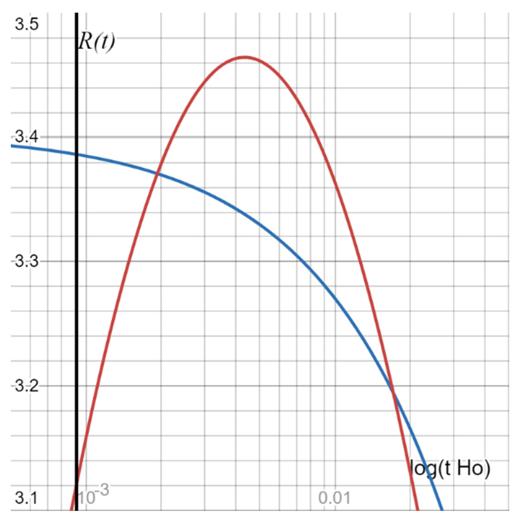
Figure 5 shows time dependence of (IN) radial R(t) and (IN) transversal D(t) distances (on a logarithmic scale for time t), and Figure 6 shows a detail of Figure 5. The vertical black line is the recombination time tCMB = 1/1090.8 for which R(tCMB) = 3.3862 and D (tCMB) = 3.1217 which gives the ratio:
3.4. Solution of Hubble tension
The Hubble tension is a 5 σ level discrepancy for the Hubble constant determined over the CMB spectrum (Planck) [2] H0 = (67.27 ± 0.60) km/s/Mpc at 68% CL and the most recent (SH0ES) values [11] H0 = (73.04 ± 1.04) km/s/Mpc at 68% CL, based on SNe Ia calibrated by Cepheids. From these data, the experimental ratio is:
A factor of 1.0847, the ratio of radial and transverse comoving distances on the CMB sphere, represents a deviation from the perfect “mimicry” of the (IN) flat universe (R/D = 1) from an IN-perspective. The experimental ratio of radial and transverse distance of the CMB sphere deviates from the theoretical (OUT) SCC value (R/D) = 1.0847 by Δ(R/D) = 0.0011, which is a confirmation of the extremely high accuracy of H0 measurements for both methods.
Of course, the direct measurement of H0 from SNe is correct, and the deviation of the H0 value obtained from the CMB measurement is due to the wrong assumption that the universe is (IN) flat.
With a correction for this theoretical factor of 1.0847, the exact value determined by the CMB measurement is H0 = (72.97 ± 0.65) km/s/Mpc. Mean value is H0(corr CMB + SNe) = (73.00 ± 0.87) km/s/Mpc. This value corresponds to the slightly lower age of the universe then from the ΛCDM model, t0 = (13.394 ± 0.160) Gy.
4. Discussion
The assumed measurement errors amount to about 1 % of the H0 values, but they are probably much smaller, because the deviation from the mean value (corr CMB + SNe) is only ΔH0 = (± 0.04) km/s/Mpc, at the relative error of 5.48∙10-4. This confirms that both series of measurements were extremely precise, accurate, which gives an answer to one, somewhat awkward question, related to the discovery of dark energy and the accelerated expansion of the universe, for which Nobel Prizes were awarded, and this paper convincingly suggests that this is “just like a mirage” of the (IN) view of a simple (OUT)-SCC universe.
Are these awards then “undeserved”? Far from it, because without the dedicated work of thousands of scientists who have been measuring this “mirage” of radial and transverse (IN) distances so precisely for years, there would be neither Kuhn's crisis in cosmology, nor this new paradigm, which is so convincing precisely because there are such precise measurements of the Hubble constant H0 determined in two different ways.
That's how science works. Old models are replaced with new ones using new paradigms based on new principes. The so-called Hubble tension, which no longer exists, confirms very precisely that we live in a 3-sphere universe with today's radius of curvature:
The so-called S8 tension is also resolved. Data from Planck TT, TE, EE + low E in combination with secondary CMB anisotropies yield
S8 = (0.834 ± 0.013), which is a factor of 1.0847 greater than the actual value. So, the CMB corrected value is
S8 = (0.769 ± 0.012) compared to a combination of local large-scale structure probes [12]
S8 = 0.766 (+0.020/-0.014). Here too, the limits of 68% CL are probably excessively large, because the deviation from their mean value
S8(corr CMB + local) = 0.7675 is (± 0.0015), at the level of the relative error of 19.5∙10-4.
The relative error of the deviation of S8 from the (corr CMB + local measurements) mean value is about 4 times higher than the relative error of the deviation of H0 from the (corr CMB + Sne measurements) mean value.
Many astronomers and astrophysicists who deal with the formation and evolution of structures of different scales in the universe do not have to doubt their theories and models, confused by the data sent by the JWST, because all these problems come down to the unexpected (incorrectly determined) early time of occurrence of these structures, earlier than previously thought.
Everything is probably fine with theories and models, especially for JWST measurements for large redshift z, because t(z) should be calculated using this simple expression t(z) = 13.394/(1+z) Gy.
For example, the galaxy JADES-GS-z14-0 has a redshift z = 14.32 (+0.08/-0.20), which is currently the most distant known galaxy. We see this galaxy when, according to ΛCDM t(z) is only 290 My after BB. The correct value is 935 My after BB.
5. Conclusion
Because all results presented in this work convincingly suggests that standard ΛCDM comology is distorted IN-side view of a much simpler SCC cosmology, I hope that this work will be an incentive and inspiration to many cosmologists for the development of this new paradigm of cosmology, new cosmological research, measurement, theorizing, questioning, and reinterpreting old and new data and models from this literally new perspective of looking at cosmology:
analogous to jumping from Geocentric to Heliocentric system. This time, I hope, much faster and more painlessly.
(IN)-ΛCDM model → (OUT)-SCC model,
Funding
This research received no external funding.
Acknowledgments
I dedicate this work to the recently deceased father, Josip Krajcar. Dad, thank you for everything!
Conflicts of Interest
The author declare no conflicts of interest.
References
- Kuhn, Thomas S. The structure of scientific revolutions (1st edition). University of Chicago Press.172.LCCN 62019621. (1962).
- Aghanim, N.; et al. , Planck 2018 results-VI. Cosmological parameters. Astronomy & Astrophysics 641, A6 (2020).
- Dahlen, T.; Strolger, L.; Riess, A.G. The ExtendedHSTSupernova Survey: The Rate of SNe Ia atz> 1.4 Remains Low. Astrophys. J. 2008, 681, 462–469. [Google Scholar] [CrossRef]
- Casado, J. Linear expansion models vs. standard cosmologies: a critical and historical overview. Astrophys. Space Sci. 2020, 365, 16. [Google Scholar] [CrossRef]
- Edward Arthur Milne,Relativity, Gravitation and World Structure, Oxford University Press. (1935).
- Melia, F.; Yennapureddy, M.K. The maximum angular-diameter distance in cosmology. Mon. Not. R. Astron. Soc. 2018, 480, 2144–2152. [Google Scholar] [CrossRef]
- Kofinas, G. The complete Brans–Dicke theories. Ann. Phys. 2017, 376, 425–435. [Google Scholar] [CrossRef]
- Barber, G.A. On two ?self-creation? cosmologies. Gen. Relativ. Gravit. 1982, 14, 117–136. [Google Scholar] [CrossRef]
- Garth, A. Barber, G.A., A New Self Creation Cosmology, Astrophysics and Space Science 282, 683-730, (2002).
- Garth, A. Barber, Self Creation Cosmology - An Alternative Gravitational Theory, New Developments in Quantum Cosmology Research. Horizons in World Physics, Volume 247, pages 155–184, Nova Science Publishers, inc. New York. (2005).
- Riess, A.G.; Yuan, W.; Macri, L.M.; Scolnic, D.; Brout, D.; Casertano, S.; Jones, D.O.; Murakami, Y.; Anand, G.S.; Breuval, L.; et al. A Comprehensive Measurement of the Local Value of the Hubble Constant with 1 km s−1 Mpc−1 Uncertainty from the Hubble Space Telescope and the SH0ES Team. Astrophys. J. 2022, 934, L7. [Google Scholar] [CrossRef]
- Heymans, C.; Tröster, T. KiDS-1000 Cosmology: Multi-probe weak gravitational lensing and spectroscopic galaxy clustering constraints. 2021; 646, A140. [Google Scholar] [CrossRef]
Disclaimer/Publisher’s Note: The statements, opinions and data contained in all publications are solely those of the individual author and contributor and not of MDPI and/or the editor. MDPI and/or the editor disclaim responsibility for any injury to people or property resulting from any ideas, methods, instructions or products referred to in the content. |
† Past employment |
⁕ Current employment |
Figure 1.
Illustration of the universe from the Big Bang to the present day, according to the ΛCDM model cosmology. (Image Credit: NASA/ LAMBDA Archive / WMAP Science Team).
Figure 1.
Illustration of the universe from the Big Bang to the present day, according to the ΛCDM model cosmology. (Image Credit: NASA/ LAMBDA Archive / WMAP Science Team).
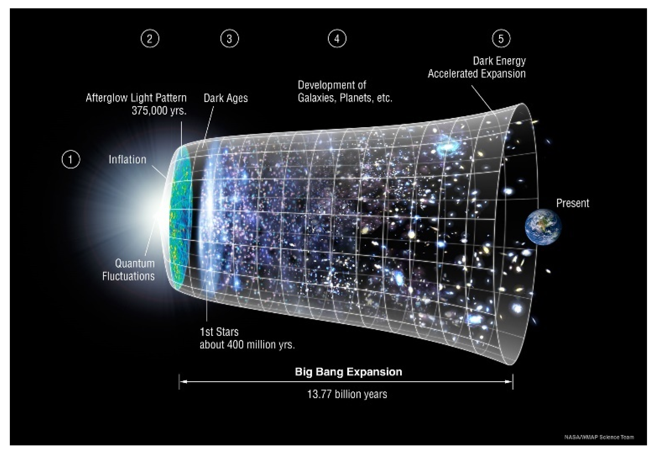
Figure 2.
Schematized representation of the (OUT) radial comoving distance R(t) for symbolic 1 year measurement, here and now with a “stair” (1 light year / 1 year) compared to the other three different “stairs”, with an enlarged detail of the middle “stair”.
Figure 2.
Schematized representation of the (OUT) radial comoving distance R(t) for symbolic 1 year measurement, here and now with a “stair” (1 light year / 1 year) compared to the other three different “stairs”, with an enlarged detail of the middle “stair”.
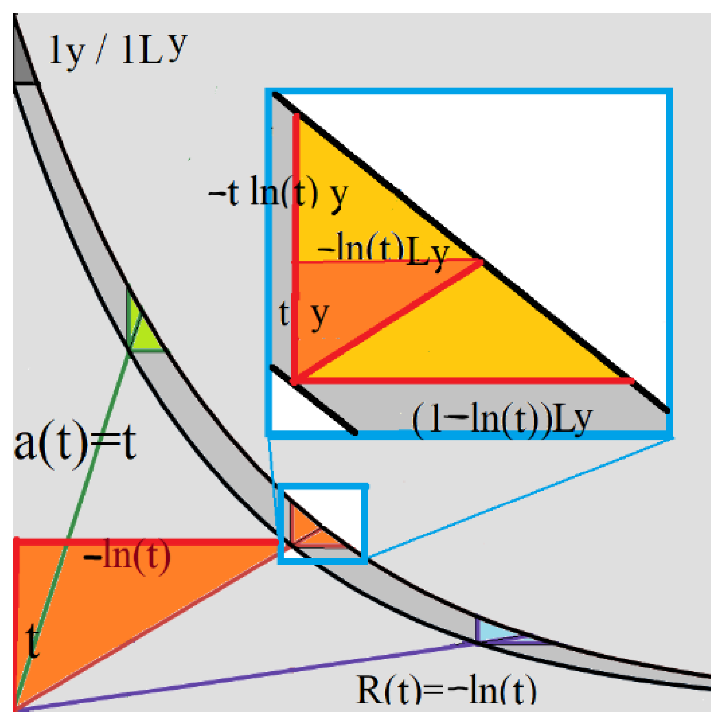
Figure 3.
Normalized (IN) T(t) (blue) and (IN) a(t) (red). The horizontal scale is the time, (t(BB)=0, t(now)=1).
Figure 3.
Normalized (IN) T(t) (blue) and (IN) a(t) (red). The horizontal scale is the time, (t(BB)=0, t(now)=1).
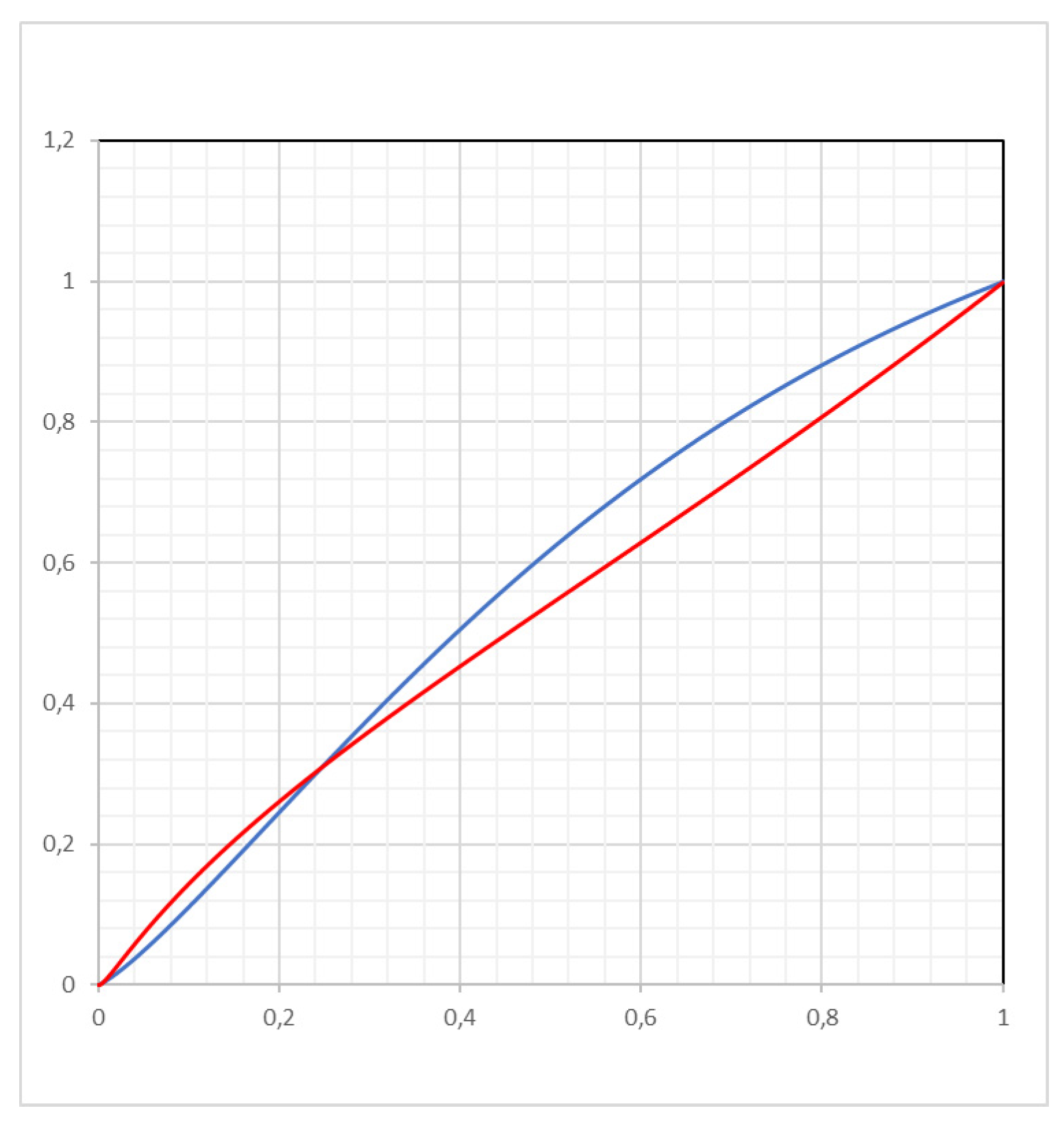
Figure 4.
The difference T(t) - T'(t) for the minimum δ(0) (blue) and δ(0.4) (red).
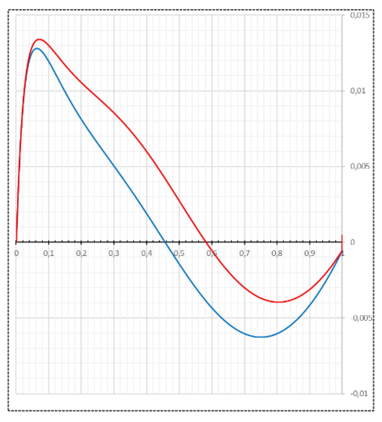
Figure 5.
Longitudinal (IN) R(t) (blue) and transversal (IN) D(t) (red) comoving distance. The time is on a logarithmic scale. Black vertical line is for t = 1/1090.8.
Figure 5.
Longitudinal (IN) R(t) (blue) and transversal (IN) D(t) (red) comoving distance. The time is on a logarithmic scale. Black vertical line is for t = 1/1090.8.
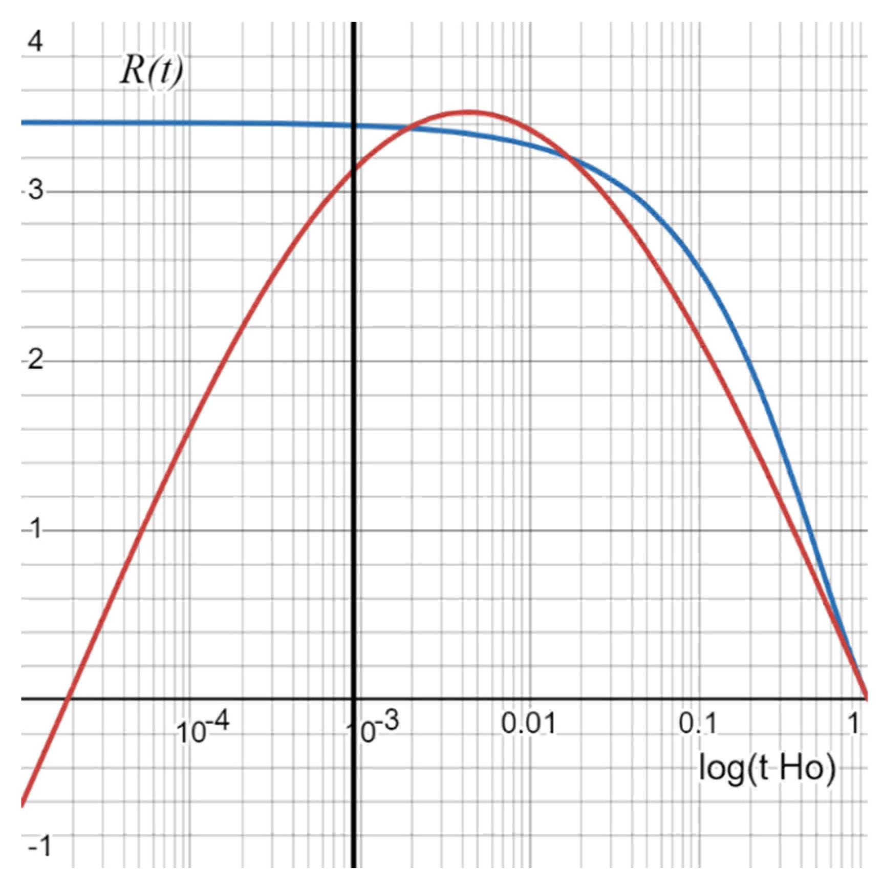
Figure 6.
Detail from Figure 5, longitudinal (IN) R(t) (blue) and transversal (IN) D(t) (red) comoving distance. The time is on a logarithmic scale. Black vertical line is for t = 1/1090.8.
Figure 6.
Detail from Figure 5, longitudinal (IN) R(t) (blue) and transversal (IN) D(t) (red) comoving distance. The time is on a logarithmic scale. Black vertical line is for t = 1/1090.8.
Disclaimer/Publisher’s Note: The statements, opinions and data contained in all publications are solely those of the individual author(s) and contributor(s) and not of MDPI and/or the editor(s). MDPI and/or the editor(s) disclaim responsibility for any injury to people or property resulting from any ideas, methods, instructions or products referred to in the content. |
© 2024 by the author. Licensee MDPI, Basel, Switzerland. This article is an open access article distributed under the terms and conditions of the Creative Commons Attribution (CC BY) license (https://creativecommons.org/licenses/by/4.0/).
Copyright: This open access article is published under a Creative Commons CC BY 4.0 license, which permit the free download, distribution, and reuse, provided that the author and preprint are cited in any reuse.


