Cosmology in Five Dimensions: A 3-Sphere Universe Without Dark Matter or Dark Energy and Its Astrophysical Applications

1. Introduction

Modern cosmology is based on the Friedmann–Lemaître–Robertson–Walker metric, or FLRW metric. This four-dimensional metric (three spatial dimensions and one temporal dimension) is considered the most general form compatible with the cosmological principle, which assumes that the universe is homogeneous and isotropic on large scales. Thanks to its scale factor a(t), the FLRW metric allows us to explain the cosmological redshift as a consequence of the expansion of the universe.

The most common form of the FLRW metric is:

$$d{s}^2=c^{2}d{t}^2-a{\left(t\right)}^2\left({\displaystyle \frac{d{r}^2}{1-k{r}^2}}+r^{2}d{\theta }^2+r^2{sin}^2\theta d{\varphi }^2\right)$$

(1)

Here, the time coordinate t is known as cosmological time, which is the proper time measured by an observer whose peculiar motion is negligible, i.e., whose motion is due only to the expansion or contraction of the homogeneous and isotropic space-time. Such observers, who all share the same cosmological time, are often referred to as fundamental observers. In an expanding universe like ours, all fundamental observers move with the Hubble flow.

The spatial coordinates (r, θ, ϕ), assigned by a fundamental observer, are called comoving coordinates and remain constant over time for any given point. The curvature parameter k can take one of three discrete values: 0, +1, or -1, corresponding respectively to flat, positively curved, or negatively curved three-dimensional hypersurfaces.

By applying Einstein’s field equations of General Relativity to the FLRW metric, one obtains the well-known Friedmann equations. These equations, given appropriate values of k and the initial matter and energy densities of the universe, describe the dynamics of the cosmos and yield a wide variety of cosmological models: open, closed, accelerating, decelerating, or even static universes. For this reason, the Friedmann equations are generally regarded as the foundational equations of modern cosmology.

To deduce them, it is sufficient to apply Einstein’s equation of General Relativity

$$G_{\alpha \beta }\equiv R_{\alpha \beta }-{\displaystyle \frac{1}{2}}R{g}_{\alpha \beta }+\Lambda g_{\alpha \beta }={\displaystyle \frac{8\pi G}{c^4}}{T}_{\alpha \beta }$$

(2)

For convenience, we will use the mixed-index form:

$$G_{\beta }^{\alpha }\equiv R_{\beta }^{\alpha }-{\displaystyle \frac{1}{2}}R{g}_{\beta }^{\alpha }+\mathsf{\Lambda }{g}_{\beta }^{\alpha }={\displaystyle \frac{8\pi G}{c^4}}{T}_{\beta }^{\alpha }$$

(3)

Assuming that the energy-momentum tensor of the universe corresponds to a perfect fluid:

$$T_{\alpha \beta }=\left(\rho +p\right)u_{\alpha }{u}_{\beta }+p{g}_{\alpha \beta }$$

(4)

If we consider that in the absence of peculiar motions, the velocity quadrivector is u^α=(1, 0, 0, 0), then the mixed energy-momentum tensor takes the form:

$$T_{\beta }^{\alpha }=\left(\begin{array}{cccc}\rho c^2& 0& 0& 0\\ 0& -p& 0& 0\\ 0& 0& -p& 0\\ 0& 0& 0& -p\end{array}\right)$$

(5)

This form of the energy-momentum tensor simplifies the calculations involving the Einstein tensor in mixed index form. Applying this setup to the FLRW metric leads directly to the two Friedmann equations:

$${\displaystyle \frac{\ddot{a}}{a}}=-{\displaystyle \frac{4\pi G}{3}}\left(\rho +3p\right)+{\displaystyle \frac{\Lambda }{3}}$$

(6)

$${\left({\displaystyle \frac{\dot{a}}{a}}\right)}^2={\displaystyle \frac{8\pi G}{3}}\rho -{\displaystyle \frac{k{c}^2}{a^2}}+{\displaystyle \frac{\Lambda }{3}}$$

(7)

2. Proposal for a New Metric of the Universe

In our approach, although the FLRW metric is considered to be the most generic possible under the cosmological principle, we will start from the metric of the 3-Sphere, whose form is:

$$\mathrm{d}{s}^2=\mathrm{d}{\mathrm{R}}^2+R^2{d\chi }^2+R^2{sin}^2\chi \mathrm{d}{\theta }^2+R^2{sin}^2\chi {sin}^2\theta \mathrm{d}{\varphi }^2$$

(8)

If we now apply the coordinate change:

$$r=\mathit{sin}\chi$$

(9)

we obtain:

$$dr=\mathit{cos}\chi d\chi$$

(10)

Squaring the expression above:

$$d{r}^2={\mathit{cos}}^2\chi d{\chi }^2=(1-{\mathit{sin}}^2\chi )d{\chi }^2$$

(11)

from which we get:

$$\mathrm{d}{\chi }^2={\displaystyle \frac{\mathrm{d}{r}^2}{\left(1-{sin}^2\chi \right)}}={\displaystyle \frac{\mathrm{d}{r}^2}{\left(1-r^2\right)}}$$

(12)

Substituting into the metric (8), we obtain the expression for the positively curved hypersphere (with k=1):

$$\mathrm{d}{s}^2=\mathrm{d}{R}^2+R^2\left({\displaystyle \frac{\mathrm{d}{r}^2}{1-r^2}}+r^2\mathrm{d}{\theta }^2+r^{2}si{n}^2\theta \mathrm{d}{\varphi }^2\right)$$

(13)

Adding the time component using the trace (+ - - - -), the full five-dimensional metric becomes:

$$\mathrm{d}{s}^2=c^2\mathrm{d}{t}^2-\mathrm{d}{R}^2-R^2\left({\displaystyle \frac{d{r}^2}{1-r^2}}+r^2\mathrm{d}{\theta }^2+r^{2}si{n}^2\theta \mathrm{d}{\varphi }^2\right)$$

(14)

Now, if we assume that the hyperspherical radius R is a function of cosmological time, R=R(ct), then its differential becomes:

$$\mathrm{d}R\left(ct\right)={\displaystyle \frac{\mathrm{d}R\left(ct\right)}{\mathrm{d}ct}}\mathrm{d}ct=\dot{R}\left(ct\right)\mathrm{d}ct=c\cdot \dot{R}\left(ct\right)\mathrm{d}t$$

(15)

(In this paper, the dot notation will be used to indicate derivatives with respect to ct.)

Substituting this into the metric gives:

$$\mathrm{d}{s}^2=c^2\mathrm{d}{t}^2-c^2\dot{R^2}\left(ct\right)\mathrm{d}{t}^2-R^2\left(ct\right)\left({\displaystyle \frac{\mathrm{d}{r}^2}{1-r^2}}+r^2\mathrm{d}{\theta }^2+r^{2}si{n}^2\theta \mathrm{d}{\varphi }^2\right)$$

(16)

Grouping time components:

$$\mathrm{d}{s}^2=\left(1-\dot{R^2}\left(ct\right)\right)c^2\mathrm{d}{t}^2-R^2\left(ct\right)\left({\displaystyle \frac{\mathrm{d}{r}^2}{1-r^2}}+r^2\mathrm{d}{\theta }^2+r^{2}si{n}^2\theta \mathrm{d}{\varphi }^2\right)$$

(17)

By comparing this expression with the standard FLRW metric (1), we see that the spatial part is equivalent under the identification a(t)=R(t). However, the temporal component differs due to its dependence on the expansion rate dR(t)/dt, which modifies the form of g_tt. As we will show later, this deviation induces a gravitational redshift that may explain the Hubble diagrams—currently interpreted as evidence for an accelerating universe—without requiring the existence of dark energy.

Assuming the energy-momentum tensor still corresponds to a perfect fluid, we write:

$$T_{\beta }^{\alpha }=\left(\begin{array}{cccc}\rho c^2& 0& 0& 0\\ 0& -p& 0& 0\\ 0& 0& -p& 0\\ 0& 0& 0& -p\end{array}\right)$$

(18)

Using the new metric (17), the Einstein’s field equations (3) give for the temporal component:

$$G_0^0={\displaystyle \frac{3}{R^2\left(ct\right)\left(1-\dot{R^2}\left(ct\right)\right)}}={\displaystyle \frac{8\pi G}{c^4}}{T}_0^0={\displaystyle \frac{8\pi G}{c^2}}\rho$$

(19)

And for the spatial diagonal components:

$$G_1^1=G_2^2=G_3^3={\displaystyle \frac{2R\left(ct\right)\ddot{R}\left(ct\right)-{\dot{R}}^2\left(ct\right)+1}{R^2\left(ct\right)(1-{\dot{R}}^2(ct){)}^2}}={\displaystyle \frac{8\pi G}{c^4}}{T}_1^1={\displaystyle \frac{8\pi G}{c^4}}{T}_2^2={\displaystyle \frac{8\pi G}{c^4}}{T}_3^3=-{\displaystyle \frac{8\pi G}{c^4}}p$$

(20)

Solving equation (19) for the denominator:

$${\displaystyle \frac{1}{R^2\left(ct\right)(1-{\dot{R}}^2(ct\left)\right)}}={\displaystyle \frac{8\pi G}{3c^2}}\rho$$

(21)

Substituting this into (20):

$${\displaystyle \frac{2R\left(ct\right)\ddot{R}\left(ct\right)-{\dot{R}}^2\left(ct\right)+1}{1-{\dot{R}}^2\left(ct\right)}}\cdot {\displaystyle \frac{8\pi G}{3c^2}}\rho =-{\displaystyle \frac{8\pi G}{c^4}}p$$

(22)

Which simplifies to:

$$p=-{\displaystyle \frac{2R\left(ct\right)\ddot{R}\left(ct\right)-{\dot{R}}^2\left(ct\right)+1}{1-{\dot{R}}^2\left(ct\right)}}\cdot {\displaystyle \frac{1}{3}}\rho c^2$$

(23)

Therefore, equations (21) and (23) can be considered the modified Friedman equations derived from the new five-dimensional hyperspherical metric (17).

3. Radiation-Dominated Universe

In this model of the Universe, the cosmological constant Λ is zero and the dominant energy density is that of radiation and relativistic matter. It is believed that a radiation-dominated universe describes well the very early stages of cosmic evolution.

If we assume that the energy density ρ_E depends on time through the scale factor R(ct), we can write:

$${\rho }_E\left(ct\right)c^2={\displaystyle \frac{E\left(ct\right)}{V\left(ct\right)}}={\displaystyle \frac{E\left(ct\right)}{\frac{4\pi }{3}{R}^3\left(ct\right)}}$$

(24)

We must now take into account that as the radius R(ct) increases, the wavelength λ of the radiation also increases, leading to a decrease in energy E(ct) inversely proportional to R(ct). To preserve correct physical dimensions, we introduce a scaling by assuming the universe is bounded by a maximum radius R_S, and define:

$$E\left(ct\right)={\displaystyle \frac{R_S}{R\left(ct\right)}}{E}_U$$

(25)

where E_U is the initial energy content of the universe.

Substituting into equation (19), we obtain:

$${\displaystyle \frac{3}{R{\left(ct\right)}^2\left(1-\dot{R^2}\left(ct\right)\right)}}={\displaystyle \frac{8\pi G}{c^4}}{\rho }_E\left(ct\right)={\displaystyle \frac{8\pi G}{c^4}}\cdot {\displaystyle \frac{E\left(ct\right)}{\frac{4\pi }{3}{R}^3\left(ct\right)}}={\displaystyle \frac{2G{E}_U}{c^4}}\cdot {\displaystyle \frac{R_S}{R^4\left(ct\right)}}$$

(26)

Reorganizing:

$${\displaystyle \frac{1}{\left(1-\dot{R^2}\left(ct\right)\right)}}={\displaystyle \frac{2G{E}_U}{c^4}}\cdot {\displaystyle \frac{R_S}{R^2\left(ct\right)}}$$

(27)

Solving for R²(ct), we get:

$$R^2\left(ct\right)={\displaystyle \frac{2G{E}_U}{c^4}}{R}_S\left(1-\dot{R^2}\left(ct\right)\right)$$

(28)

Now, defining:

$$R_S={\displaystyle \frac{2G{E}_U}{c^4}}$$

(29)

we obtain a clean expression:

$$R\left(ct\right)=R_S\sqrt{1-\dot{R^2}\left(ct\right)}$$

(30)

From this, we can isolate the velocity of expansion:

$$\dot{R}\left(ct\right)=\sqrt{1-{\displaystyle \frac{R^2\left(ct\right)}{R_S^2}}}$$

(31)

This implies that R(ct) ≤ R_S as expected.

Figure 1. The rate of expansion of the universe as a function of its radius R(t).

Figure 1. The rate of expansion of the universe as a function of its radius R(t).

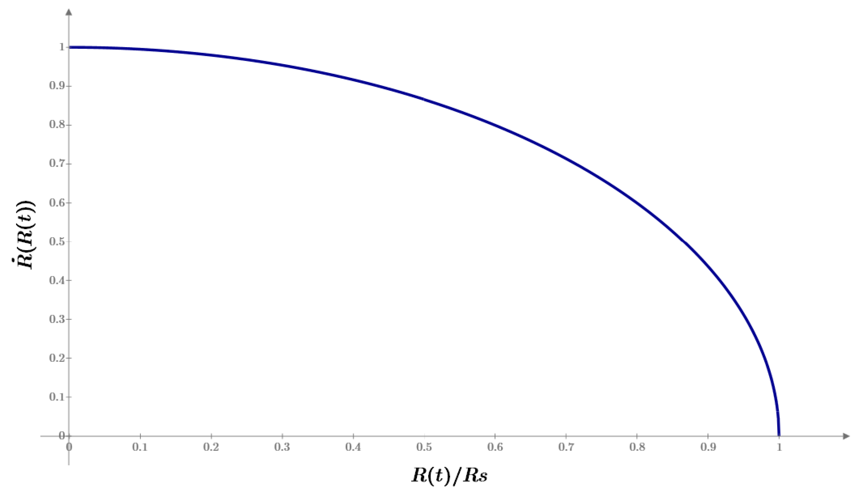
If we now derive the expression (31) again we will obtain:

$$\ddot{R}\left(ct\right)={\displaystyle \frac{-2R\left(ct\right)\dot{R}\left(ct\right)}{R_S^2\cdot 2\sqrt{1-\frac{R^2\left(ct\right)}{R_S^2}}}}={\displaystyle \frac{-R\left(ct\right)}{R_S^2}}$$

(32)

This shows that the universe is expanding with a deceleration caused by the gravitational pull of its own energy content E_U.

If we now substitute equations (31) and (32) into equation (23) we obtain:

$$p=-{\displaystyle \frac{\frac{-2R^2\left(ct\right)}{R_S^2}-\left(1-\frac{R^2\left(ct\right)}{R_S^2}\right)+1}{1-\dot{R^2}\left(ct\right)}}\cdot {\displaystyle \frac{1}{3}}\rho c^2={\displaystyle \frac{R^2\left(ct\right)}{R_S^2\left(1-\dot{R^2}\left(ct\right)\right)}}\cdot {\displaystyle \frac{1}{3}}\rho c^2$$

(33)

And if we take into account (30) then we finally recover:

$$p={\displaystyle \frac{1}{3}}\rho c^2$$

(34)

which is the expected equation of state for a radiation-dominated universe.

We can now integrate the equation (31) by introducing the change of variable:

$${\displaystyle \frac{R\left(ct\right)}{R_S}}=\sin x$$

(35)

Assuming that the universe starts at R(0) = 0, we find:

$$R\left(ct\right)=R_{S}sin\left({\displaystyle \frac{ct}{R_S}}\right)$$

(36)

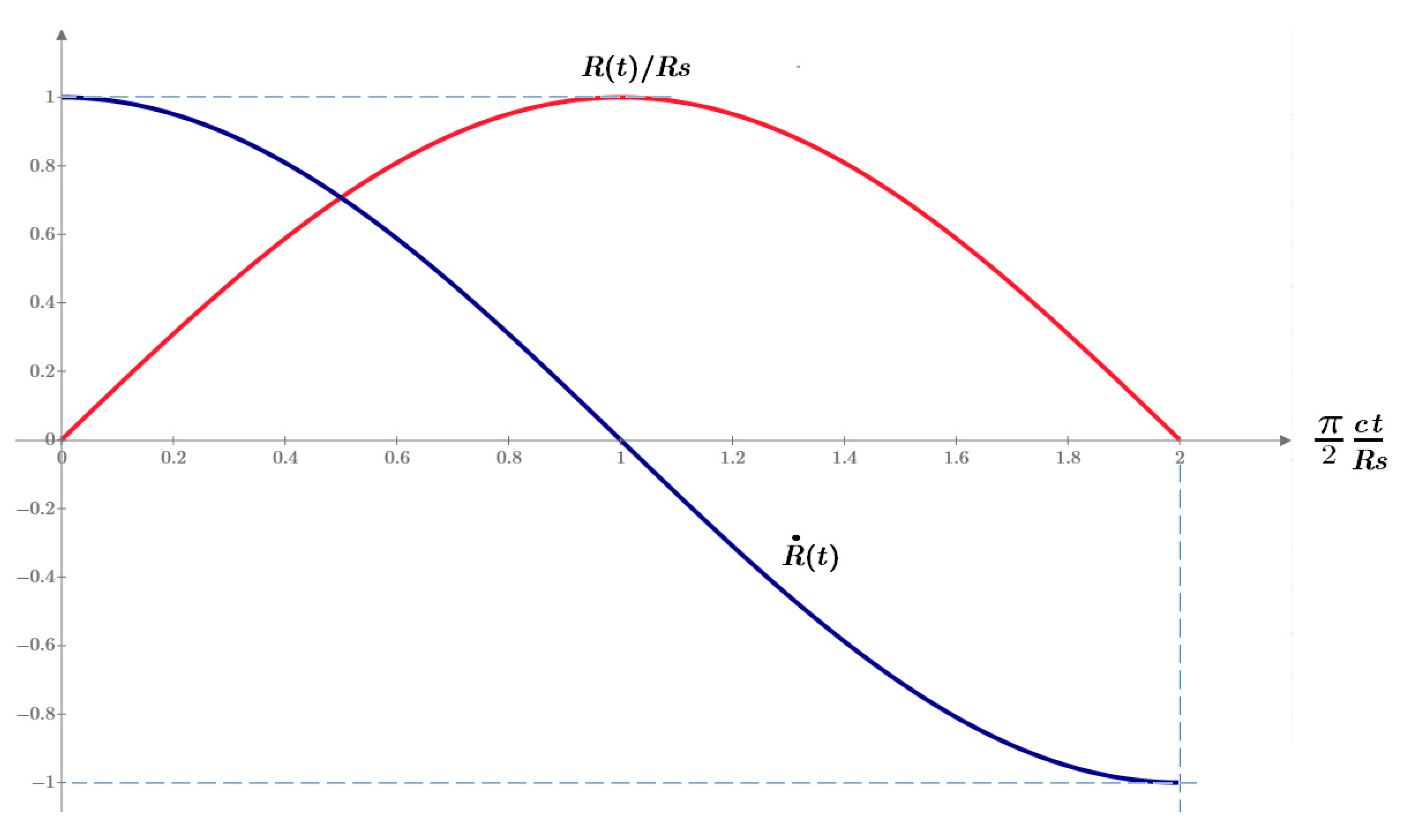
Differentiating with respect to ct:

$$\dot{R}\left(ct\right)=cos\left({\displaystyle \frac{ct}{R_S}}\right)$$

(37)

and:

$$\ddot{R}\left(ct\right)={\displaystyle \frac{-1}{R_S}}sin\left({\displaystyle \frac{ct}{R_S}}\right)$$

(38)

From these expressions, we deduce that the universe begins with zero radius and an initial expansion velocity equal to the speed of light, c, which gradually decreases to zero at:

$$ct={\displaystyle \frac{\pi }{2}}\cdot R_S$$

(39)

After this point, the universe would enter a contraction phase, eventually returning to zero size.

Figure 2. Expansion rate (blue) and size of the universe (red) as a function of cosmological time t.

Figure 2. Expansion rate (blue) and size of the universe (red) as a function of cosmological time t.

If we now substitute equation (31) in the metric (17), we get:

$$\mathrm{d}{s}^2={\displaystyle \frac{R^2\left(ct\right)}{R_S^2}}{c}^2\mathrm{d}{t}^2-R^2\left(ct\right)\left({\displaystyle \frac{\mathrm{d}{r}^2}{1-r^2}}+r^2\mathrm{d}{\theta }^2+r^{2}si{n}^2\theta \mathrm{d}{\varphi }^2\right)$$

(40)

Replacing with equation (37):

$$\mathrm{d}{s}^2={sin}^2\left({\displaystyle \frac{ct}{R_S}}\right)c^2\mathrm{d}{t}^2-R_S^2{sin}^2\left({\displaystyle \frac{ct}{R_S}}\right)\left({\displaystyle \frac{\mathrm{d}{r}^2}{1-r^2}}+r^2\mathrm{d}{\theta }^2+r^{2}si{n}^2\theta \mathrm{d}{\varphi }^2\right)$$

(41)

Defining a new time coordinate τ:

$$\mathrm{d}\tau =sin\left({\displaystyle \frac{ct}{R_S}}\right)\mathrm{d}t$$

(42)

we recover the FLRW form:

$$\mathrm{d}{s}^2=c^2\mathrm{d}{\tau }^2-R^2\left(\tau \right)\left({\displaystyle \frac{\mathrm{d}{r}^2}{1-r^2}}+r^2\mathrm{d}{\theta }^2+r^{2}si{n}^2\theta \mathrm{d}{\varphi }^2\right)$$

(43)

Integrating both sides of (42):

$$\tau =-{\displaystyle \frac{R_S}{c}}cos\left({\displaystyle \frac{ct}{R_S}}\right)+C$$

(44)

With τ = 0 when t = 0, then we can calculate the value of C to have

$$\tau ={\displaystyle \frac{R_S}{c}}\left(1-cos\left({\displaystyle \frac{ct}{R_S}}\right)\right)$$

(45)

Solving for t as a function of τ:

$$t={\displaystyle \frac{R_S}{c}}\cdot arccos\left(1-{\displaystyle \frac{c\tau }{R_S}}\right)$$

(46)

We can now evaluate the expansion velocity in terms of τ by differentiating (37):

$$\dot{R}\left(ct\right)={\displaystyle \frac{\mathrm{d}R}{\mathrm{d}ct}}={\displaystyle \frac{\mathrm{d}R}{\mathrm{d}c\tau }}\cdot {\displaystyle \frac{\mathrm{d}c\tau }{\mathrm{d}ct}}=\dot{R}\left(c\tau \right){\displaystyle \frac{\mathrm{d}\tau }{\mathrm{d}t}}=\dot{R}\left(c\tau \right){\displaystyle \frac{R\left(ct\right)}{R_S}}=\sqrt{1-{\displaystyle \frac{R^2\left(ct\right)}{R_S^2}}}$$

(47)

Then:

$$\dot{R}\left(c\tau \right)=\sqrt{{\displaystyle \frac{R_S^2}{R^2\left(c\tau \right)}}-1}$$

(48)

Differentiating again:

$$\ddot{R}\left(c\tau \right)=-{\displaystyle \frac{R_S^2}{R^3\left(c\tau \right)}}$$

(49)

Substituting from (29):

$$\ddot{R}\left(\tau \right)=-{\displaystyle \frac{{\left(\frac{2G{E}_U}{c^4}\right)}^2}{R^3\left(\tau \right)}}$$

(50)

Finally, integrating:

$$c\mathrm{d}\tau ={\displaystyle \frac{\mathrm{d}R\left(c\tau \right)}{\sqrt{\frac{R_S^2}{R^2\left(c\tau \right)}-1}}}$$

(51)

we obtain:

$$R\left(\tau \right)=\sqrt{2c\tau R_S-c^2{\tau }^2}$$

(52)

4. Universe Dominated by Non-Relativistic Matter

Once the universe has expanded enough, the energy density of radiation —which scales as R⁻⁴— decreases faster than the energy density of non-relativistic (or "dust") matter, which scales as R⁻³. Therefore, a transition occurs where the matter component becomes dominant, and the equations obtained for the radiation-dominated epoch are no longer valid.

Assuming again that the cosmological constant vanishes and that the total mass of the universe is a conserved quantity M_U, the matter density evolves as:

$${\rho }_M\left(t\right)={\displaystyle \frac{M_U}{V\left(t\right)}}={\displaystyle \frac{M_U}{\frac{4\pi }{3}{R}^3\left(ct\right)}}$$

(53)

Substituting into the equation (21) we will have:

$${\displaystyle \frac{3}{R^2\left(ct\right)\left(1-\dot{R^2}\left(ct\right)\right)}}={\displaystyle \frac{8\pi G}{c^2}}\cdot {\displaystyle \frac{M_U}{\frac{4\pi }{3}{R}^3\left(ct\right)}}={\displaystyle \frac{2G{M}_U}{c^2}}\cdot {\displaystyle \frac{3}{R^3\left(ct\right)}}$$

(54)

If we define R_S as (note the equality with the Schwarzschild radius):

$$R_S={\displaystyle \frac{2G{M}_U}{c^2}}$$

(55)

then equation (54) simplifies to:

$${\displaystyle \frac{1}{1-{\dot{R}}^2\left(ct\right)}}={\displaystyle \frac{R_S}{R\left(ct\right)}}$$

(56)

Rewriting:

$$R\left(ct\right)=R_S\left(1-\dot{R^2}\left(ct\right)\right)$$

(57)

Solving for the velocity of expansion:

$$\dot{R}\left(ct\right)=\sqrt{1-{\displaystyle \frac{R\left(ct\right)}{R_S}}}$$

(58)

This immediately implies a bound on the expansion: R(ct) < R_S, that is, the hyperradial expansion

cannot exceed the Schwarzschild radius determined by M_U.

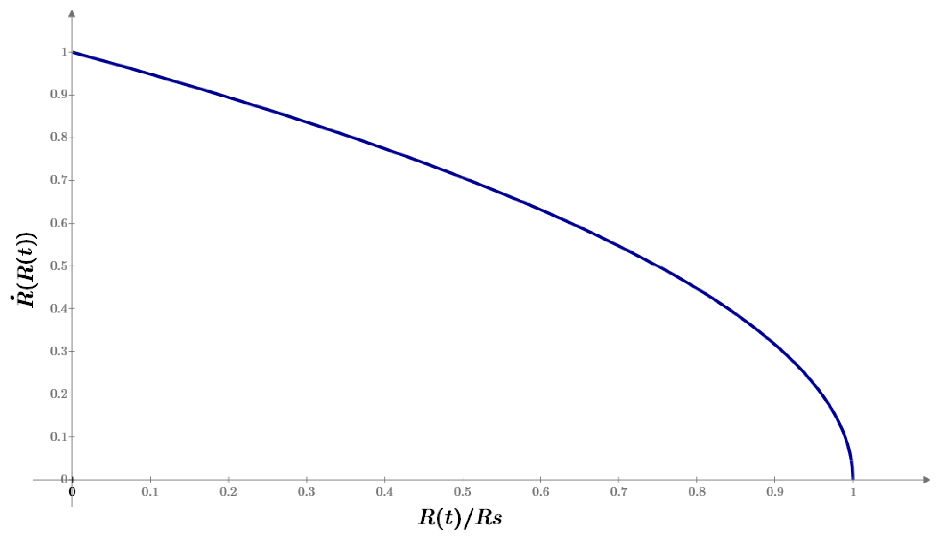
Taking the time derivative of (58):

$$\ddot{R}\left(ct\right)={\displaystyle \frac{-\dot{R}\left(ct\right)}{{2 R}_S\cdot \sqrt{1-\frac{R\left(ct\right)}{R_S}}}}={\displaystyle \frac{-1}{2R_S}}$$

(59)

This result shows that the universe decelerates under the influence of its own gravity, in full analogy with Newtonian cosmology.

Subtituting equations (58) and (59) into the pressure equation (23):

$$p=-{\displaystyle \frac{\frac{2R\left(ct\right)}{-2R_S}-\left(1-\frac{R\left(ct\right)}{R_S}\right)+1}{1-\dot{R^2}\left(ct\right)}}\cdot {\displaystyle \frac{1}{3}}\rho c^2=-{\displaystyle \frac{0}{1-\dot{R^2}\left(ct\right)}}\cdot {\displaystyle \frac{1}{3}}\rho c^2=0$$

(60)

Figure 3. Dependence of the expansion rate of the universe on its radius R(t).

Figure 3. Dependence of the expansion rate of the universe on its radius R(t).

So we recover the expected result for a pressureless (dust) universe:

$$p=0$$

(61)

We can now integrate the equations (58) and (59) to obtain the functional form of the expansion:

$$R\left(ct\right)=ct-{\displaystyle \frac{{\left(ct\right)}^2}{4R_S}}$$

(62)

Solving this for t:

$$t\left(R\right)={\displaystyle \frac{2R_S}{c}}\left(1-\sqrt{1-{\displaystyle \frac{R}{R_S}}}\right)$$

(63)

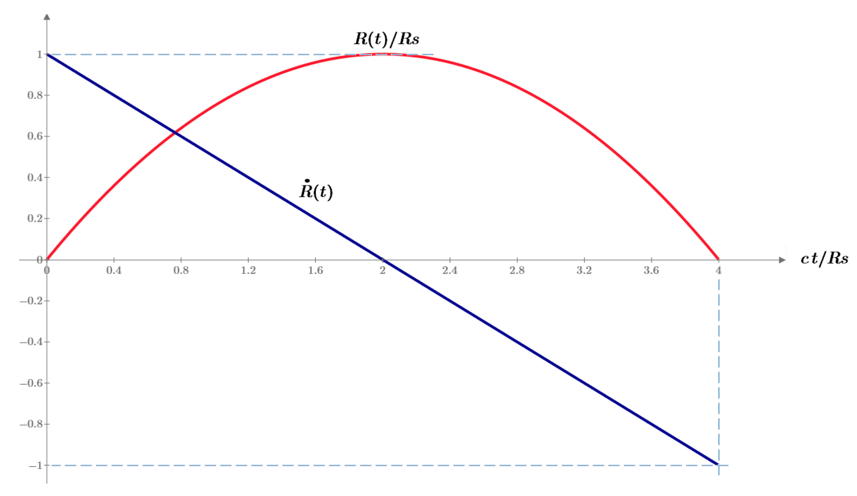
From (62), the velocity becomes:

$$\dot{R}\left(ct\right)=1-{\displaystyle \frac{ct}{2R_S}}$$

(64)

This shows that the universe starts from a size R(0) = 0 and an expansion velocity equal to the speed of light, c, decelerates linearly, and comes to a halt at:

$$t={\displaystyle \frac{2R_S}{c}}$$

(65)

Beyond that, the solution implies a re-collapse at:

$$R\left({\displaystyle \frac{4R_S}{c}}\right)=0$$

(66)

Figure 4. Expansion rate (blue) and size of the universe (red) as a function of cosmological time t.

Figure 4. Expansion rate (blue) and size of the universe (red) as a function of cosmological time t.

Finally, if we replace (58) in the expression (17) of the metric we obtain:

$$\mathrm{d}{s}^2={\displaystyle \frac{R\left(ct\right)}{R_S}}{c}^2\mathrm{d}{t}^2-R^2\left(ct\right)\left({\displaystyle \frac{\mathrm{d}{r}^2}{1-r^2}}+r^2\mathrm{d}{\theta }^2+r^{2}si{n}^2\theta \mathrm{d}{\varphi }^2\right)$$

(67)

We now define the proper time τ for a comoving observer as:

$$\mathrm{d}\tau =\sqrt{{\displaystyle \frac{R\left(t\right)}{R_S}}}\mathrm{d}t$$

(68)

Which transforms the metric into the standard FLRW form:

$$\mathrm{d}{s}^2=c^2\mathrm{d}{\tau }^2-R^2\left(c\tau \right)\left({\displaystyle \frac{\mathrm{d}{r}^2}{1-r^2}}+r^2\mathrm{d}{\theta }^2+r^{2}si{n}^2\theta \mathrm{d}{\varphi }^2\right)$$

(69)

Substituting (62) into (68), we find:

$$\int \mathrm{d}\tau =\int \sqrt{{\displaystyle \frac{R\left(ct\right)}{R_S}}}\mathrm{d}t=\int \sqrt{{\displaystyle \frac{ct-\frac{{\left(ct\right)}^2}{4R_S}}{R_S}}}\mathrm{d}t={\displaystyle \frac{1}{2R_S}}\int \sqrt{4R_S\cdot ct-{\left(ct\right)}^2}\mathrm{d}t$$

(70)

This integral yields:

$$\tau ={\displaystyle \frac{R_S}{c}}arcsin\left({\displaystyle \frac{ct-2R_S}{2R_S}}\right)+{\displaystyle \frac{ct-2R_S}{4R_S\cdot c}}\sqrt{4R_{S}ct-c^2{t}^2}+C$$

(71)

And if we assume that τ = 0 when t = 0 then we obtain:

$$\tau ={\displaystyle \frac{R_S}{c}}arcsin\left({\displaystyle \frac{ct-2R_S}{2R_S}}\right)+{\displaystyle \frac{ct-2R_S}{4R_S\cdot c}}\sqrt{4R_{S}ct-c^2{t}^2}-{\displaystyle \frac{3\pi }{2}}\cdot {\displaystyle \frac{R_S}{c}}$$

(72)

From this, we can compute the velocity in R with respect to proper time τ:

$$\dot{R}\left(ct\right)={\displaystyle \frac{\mathrm{d}R}{\mathrm{d}ct}}={\displaystyle \frac{\mathrm{d}R}{\mathrm{d}c\tau }}{\displaystyle \frac{\mathrm{d}c\tau }{\mathrm{d}ct}}=\dot{R}\left(c\tau \right){\displaystyle \frac{\mathrm{d}\tau }{\mathrm{d}t}}=\dot{R}\left(c\tau \right)\sqrt{{\displaystyle \frac{R\left(ct\right)}{R_S}}}=\sqrt{{\displaystyle \frac{R_S-R\left(ct\right)}{R_S}}}$$

(73)

then we can clear:

$${\displaystyle \frac{\mathrm{d}R\left(c\tau \right)}{\mathrm{d}c\tau }}=\dot{R}\left(c\tau \right)=\sqrt{{\displaystyle \frac{R_S-R\left(ct\right)}{R\left(ct\right)}}}=\sqrt{{\displaystyle \frac{R_S-R\left(c\tau \right)}{R\left(c\tau \right)}}}$$

(74)

And if we derive again with respect to cτ we obtain that:

$$\ddot{R}\left(c\tau \right)={\displaystyle \frac{1}{2\cdot \sqrt{\frac{R_S-R\left(c\tau \right)}{R\left(c\tau \right)}}}}\cdot {\displaystyle \frac{-\dot{R}\left(c\tau \right)\left(R\right(c\tau )+R_S-R(c\tau \left)\right)}{R^2\left(c\tau \right)}}={\displaystyle \frac{-R_S}{2R^2\left(c\tau \right)}}={\displaystyle \frac{-R_S}{2R^2\left(c\tau \right)}}$$

(75)

If we now substitute the value of R_S given by (55) we get:

$$\ddot{R}\left(\tau \right)={\displaystyle \frac{-c^2{R}_S}{2R^2\left(\tau \right)}}={\displaystyle \frac{2G{M}_U}{c^2}}\cdot {\displaystyle \frac{-c^2}{2R^2\left(\tau \right)}}=-{\displaystyle \frac{G{M}_U}{R^2\left(\tau \right)}}$$

(76)

This is precisely the Newtonian gravitational acceleration produced by the total mass M_U.

Finally, if we take into account (74) then we can clear:

$$c\mathrm{d}\tau =\sqrt{{\displaystyle \frac{R\left(c\tau \right)}{R_S-R\left(c\tau \right)}}}\cdot \mathrm{d}R\left(c\tau \right)$$

(77)

which leads to:

$$\tau \left(R\right)={\displaystyle \frac{R_S}{c}}arctan\left(\sqrt{{\displaystyle \frac{R}{R_S-R}}}\right)-{\displaystyle \frac{\left(R_S-R\right)}{c}}\sqrt{{\displaystyle \frac{R}{R_S-R}}}$$

(78)

4.1. Proper Distance and Hubble’s Law

If we start from the metric (69) with the proper time τ in which we assume that angular coordinates, θ and ϕ, don’t change, then:

$$d{s}^2=c^{2}d{\tau }^2-R^2\left(\tau \right)d{\chi }^2$$

(79)

If we define

$$\mathrm{d}\sigma =R\left(\tau \right)\mathrm{d}\chi$$

(80)

then for an observer with time τ who tries to determine the spatial distance σ(τ) along the coordinate χ (radial coordinate) we will have

$$\sigma \left(\tau \right)={\int }_0^{\chi }R\left(\tau \right)\mathrm{d}\chi =R\left(\tau \right)\chi$$

(81)

Now we can define the proper radial velocity, v_p, as:

$$v_p={\displaystyle \frac{\mathrm{d}\sigma \left(\tau \right)}{d\tau }}={\displaystyle \frac{\mathrm{d}R\left(\tau \right)}{\mathrm{d}\tau }}\chi =\dot{R}\left(\tau \right)\chi$$

(82)

And if from (81) we clear χ:

$$\chi ={\displaystyle \frac{\sigma \left(\tau \right)}{R\left(\tau \right)}}$$

(83)

then we can substitute in (82) and obtain:

$$v_p={\displaystyle \frac{\dot{R}\left(\tau \right)}{R\left(\tau \right)}}\sigma \left(\tau \right)=H\left(\tau \right)\cdot \sigma \left(\tau \right)$$

(84)

where we arrive to the law of velocity-distance, with the Hubble parameter, H(τ).

Now we can use (74) to get that the Hubble parameter would be:

$$H\left(\tau \right)=c\cdot \sqrt{{\displaystyle \frac{R_S-R\left(\tau \right)}{R\left(\tau \right)}}}\cdot {\displaystyle \frac{1}{R\left(\tau \right)}}=c\cdot \sqrt{{\displaystyle \frac{R_S-R\left(\tau \right)}{R^3\left(\tau \right)}}}$$

(85)

From the above expression we can operate a little and obtain:

$$R^3\left(\tau \right)\cdot {\displaystyle \frac{H^2\left(\tau \right)}{c^2}}+R\left(\tau \right)–R_S=0$$

(86)

which allows us to calculate the value of R(τ) as a function of H(τ) and R_S by solving the above equation of the third degree.

Let’s put some numbers to the above amounts. Let’s suppose that

$$M_U=1.51\cdot {10}^{53}\mathrm{k}\mathrm{g}$$

(87)

then we get that

$$R_S=2.2411\cdot {10}^{26}\mathrm{m}=23.70\cdot {10}^9\mathrm{l}\mathrm{i}\mathrm{g}\mathrm{h}\mathrm{t}-\mathrm{y}\mathrm{e}\mathrm{a}\mathrm{r}\mathrm{s}$$

(88)

If we take the value

$$\mathrm{H}\left(\mathsf{\tau }\right)=70.4{\displaystyle \frac{\mathrm{km}}{\mathrm{s}·\mathrm{Mpc}}}$$

(89)

we can solve (86) to get that the current value of R(τ) is

$$R\left(\tau \right)=R\left(t\right)=1.212\cdot {10}^{26}\mathrm{m}=12.81\cdot {10}^9\mathrm{l}\mathrm{i}\mathrm{g}\mathrm{h}\mathrm{t}-\mathrm{y}\mathrm{e}\mathrm{a}\mathrm{r}\mathrm{s}$$

(90)

Now we can use (63) to obtain the current coordinate time t as:

$$t=15.27\cdot {10}^9\mathrm{y}\mathrm{e}\mathrm{a}\mathrm{r}\mathrm{s}$$

(91)

and (78) to have the current proper time τ as:

$$\tau =7.767\cdot {10}^9\mathrm{y}\mathrm{e}\mathrm{a}\mathrm{r}\mathrm{s}$$

(92)

Now we can use expressions (73) and (74) to calculate the expansion velocity of the universe in the coordinate R to obtain values of 0.69 c for the coordinate observer, and 0.95 c for a comoving observer.

Finally, we can represent graphically in the area in which H(τ) takes the range of values among which it is considered to be at present:

Figure 5. The value of the Hubble constant as a function of the size of the universe.

Figure 5. The value of the Hubble constant as a function of the size of the universe.

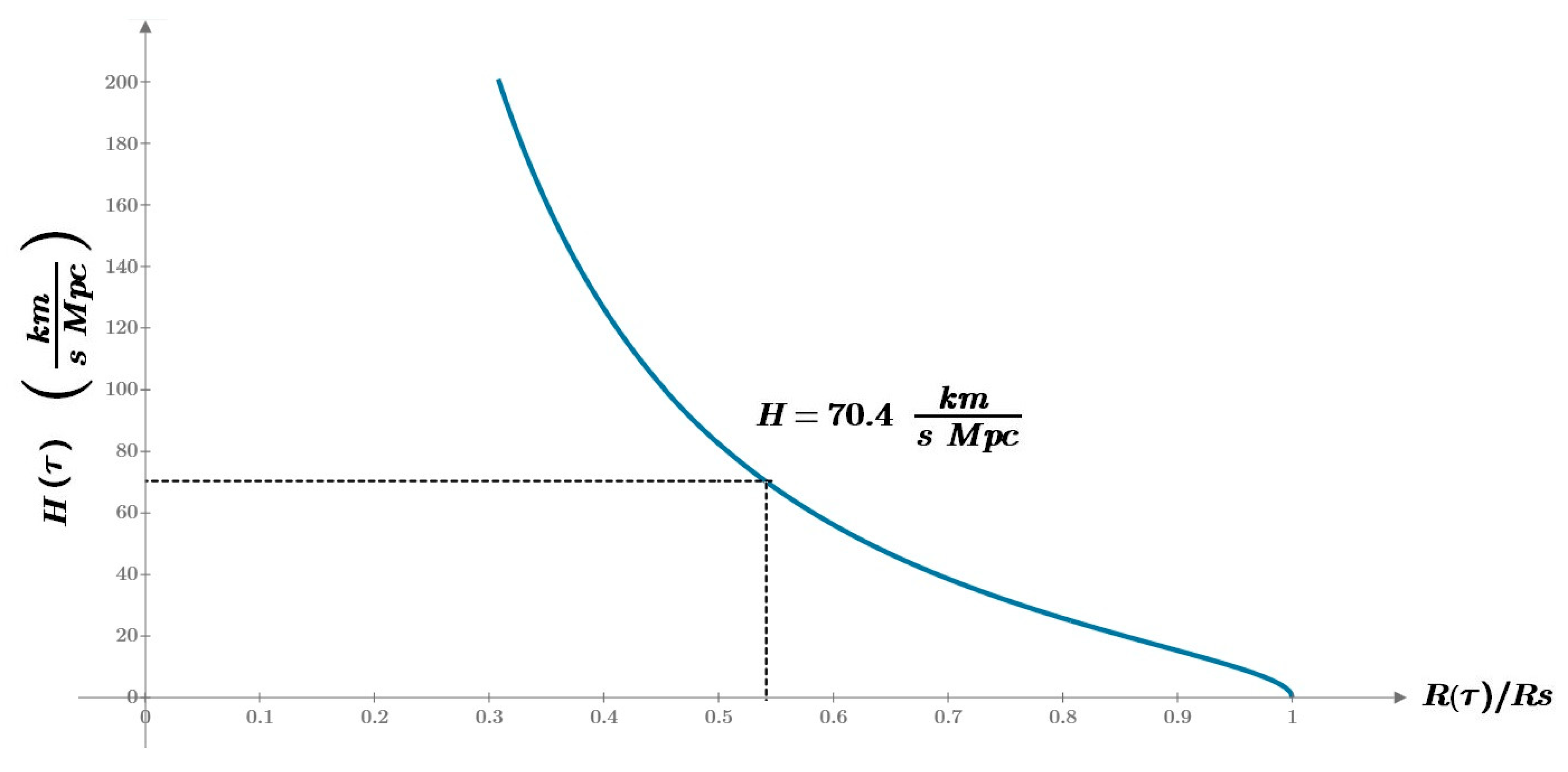
Figure above shows the behavior of the Hubble parameter H(τ) as a function of the Universe’s radius R(τ), normalized to the total Schwarzschild radius R_S. The current observed value H(τ₀) = 70.4 km/s/Mpc is indicated, which corresponds to a Universe radius of R(τ₀)/R_S ≈ 54.1%, and consistent with an ongoing expansion. As the radius increases, H(τ) decreases monotonically, tending to zero at R(τ) = R_S, which would mark the turnaround point of the expansion.

4.2. Cosmological Acceleration

In the expression (76) we have obtained that, for a universe dominated by matter, there is a proper acceleration in the radial direction R of expansion that coincides with the gravitational acceleration generated by the total mass of the universe M_U. This acceleration, which from now on we will call cosmological acceleration g_C(τ), is given by:

$$g_C\left(\tau \right)\equiv \ddot{R}\left(\tau \right)=-{\displaystyle \frac{G{M}_U}{R^2\left(\tau \right)}}$$

(76)

The fact that cosmological acceleration occurs in the direction of R, which is one additional spatial dimension, unlike the usual expansion encoded in the FLRW scale factor a(t), allows us to suggest that part of this acceleration could be transmitted or projected onto the other spatial dimensions. Let us explore this idea.

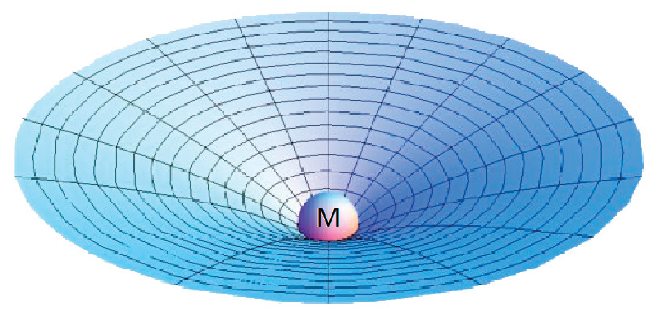
By analogy, let us imagine that our universe is confined to the surface of a 2D sphere embedded in 3D space. In the presence of massive objects, such as stars or galaxies, this surface will undergo local deformations. These deformations, in the weak field limit, can be modeled by the Schwarzschild metric. Restricting to a 2D section, the embedding of this metric in 3D Euclidean space results in the well-known Flamm’s paraboloid.

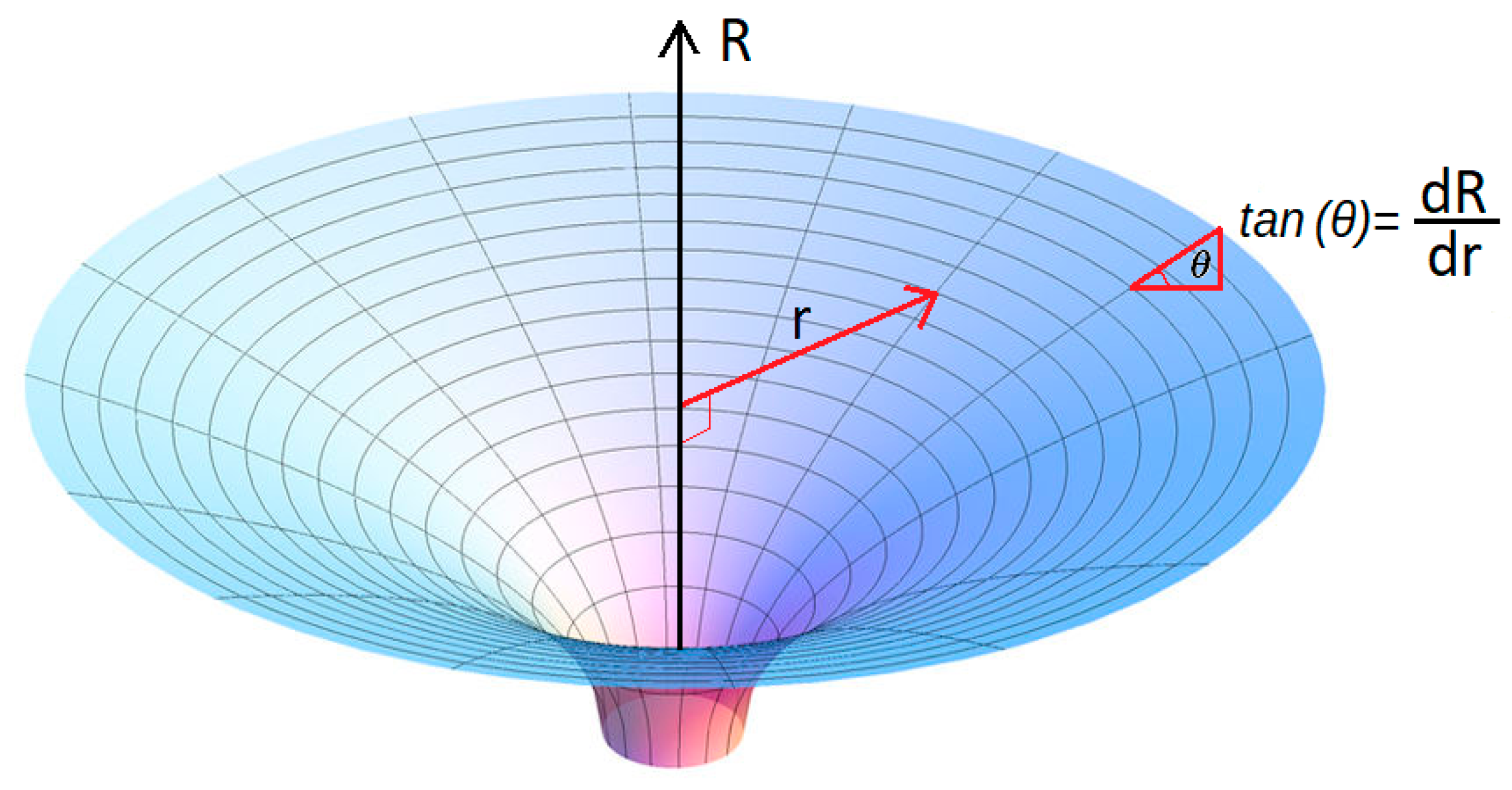
If we assume the above as correct, we may consider that part of the cosmological acceleration g_C(τ) could be projected into the radial coordinate r, affected by the slope of the paraboloid. To do this, it is enough to multiply g_C(τ) by sin(θ) where θ is the angle between the tangent to the paraboloid and the equatorial plane, as shown in the figure below.

From Flamm’s paraboloid, the slope at each point r is:

$$\mathrm{t}\mathrm{a}\mathrm{n}\left(\theta \right)={\displaystyle \frac{dR\left(\tau \right)}{dr}}=\sqrt{g_{rr}\left(r\right)-1}=\sqrt{{\displaystyle \frac{R_S}{r-R_S}}}$$

(93)

where R_S is now the Schwarzschild radius generated by the mass M_g located at r = 0:

$$R_s={\displaystyle \frac{2G{M}_g}{c^2}}$$

(94)

and g_rr(r) is the radial component of the metric.

Figure 6. Flamm’s paraboloid in a 2D universe.

Figure 6. Flamm’s paraboloid in a 2D universe.

For r much bigger than R_S (let’s think that the mass M necessary to obtain a R_S of 1 Kpc would be of M > 1·10¹⁶ solar masses) we can approximate:

$$\mathrm{s}\mathrm{i}\mathrm{n}\left(\theta \right)\simeq \tan \left(\theta \right)$$

(95)

Therefore, the projected acceleration becomes:

$$g_r\left(\tau \right)=\sin (\theta \left)g_C\right(\tau )\simeq {\displaystyle \frac{dR\left(\tau \right)}{dr}}{g}_C(\tau )=\sqrt{g_{rr}-1}\cdot g_C(\tau )=\sqrt{{\displaystyle \frac{R_s}{r-R_s}}}\cdot {\displaystyle \frac{-G{M}_U}{R^2\left(\tau \right)}}$$

(96)

an expression that for r much greater than R_S can be approximated to:

$$g_r\left(r\right)\simeq \sqrt{{\displaystyle \frac{R_s}{r}}}\cdot {\displaystyle \frac{-G{M}_u}{R_U^2}}$$

(97)

where we have assumed that the universe ratio, R(τ), remains approximately constant, so we have defined R_U = R(τ).

Figure 7. Diagram with the tan(θ) in a Flamm paraboloid.

Figure 7. Diagram with the tan(θ) in a Flamm paraboloid.

Now we write the condition of centripetal balance for an object of mass m rotating in a circular orbit at distance r:

$$\mathrm{m}{\displaystyle \frac{v^2\left(r\right)}{r}}=\mathrm{m}\cdot g_N\left(r\right)+\mathrm{m}\cdot g_r\left(r\right)={\displaystyle \frac{G{M}_{g}m}{r^2}}+\mathrm{m}\sqrt{{\displaystyle \frac{R_s}{r}}}\cdot {\displaystyle \frac{G{M}_U}{R_U^2}}$$

(98)

where g_N(r) is the acceleration of gravity according to Newton.

If now, for very large r, we ignore the part due to Newton’s acceleration of gravity since it has a dependence on 1/r² compared to the dependence 1/r^1/2 of the second summation, we will obtain what we can define as cosmological velocity, v_C(r):

$$v_C^2\left(r\right)=\sqrt{{\displaystyle \frac{R_s}{r}}}\cdot {\displaystyle \frac{G{M}_U}{R_U^2}}\mathrm{r}={\displaystyle \frac{G{M}_U}{R_U^2}}\sqrt{R_{s}r}=g_C\left(\mathsf{\tau }\right)\sqrt{R_{s}r}$$

(99)

And if we take the square root to obtain v_C(r):

$$v_C\left(r\right)=\sqrt{g_C\left(\tau \right)}\cdot \sqrt[4]{R_{s}r}$$

(100)

Subtituting the value of R_S of equation (94) we get:

$${\mathrm{v}}_{\mathrm{C}}\left(\mathrm{r}\right)=\sqrt{{\mathrm{g}}_{\mathrm{C}}\left(\mathsf{\tau }\right)}\cdot \sqrt[4]{r{\displaystyle \frac{2G{M}_g}{c^2}}}=\sqrt{{\displaystyle \frac{G{M}_U}{R_U^2}}}\cdot \sqrt[4]{r{\displaystyle \frac{2G{M}_g}{c^2}}}$$

(101)

From here, we can solve for the galaxy mass M_g:

$${\mathrm{M}}_{\mathrm{g}}=v_C^4\cdot {\displaystyle \frac{c^2{R}_U^4}{2G^3{M}_U^{2}r}}$$

(102)

that is, M_g is proportional to:

$${\mathrm{M}}_{\mathrm{g}}\propto {\displaystyle \frac{v_c^4}{r}}\propto v_c^4$$

(103)

The expression (103) shows that the mass of a galaxy is proportional to the fourth power of the rotation velocity v_c(r), which is the essence of the Tully-Fisher relation [1]. However, an undesired residual dependence on the radial coordinate r remains. This is due to the fact that the velocity expression in (101) grows as r^1/4 instead of tending to a constant.

4.3. Formal Derivation of the Cosmological Acceleration Projected onto the 3D Universe

Although the explanation in the previous section is highly visual and intuitive, it is necessary to demonstrate, mathematically and via the metric, that the radial acceleration indeed includes a term generated by the cosmological acceleration.

To do so, we start with the following form of our metric, equation (14), where we have simply replaced the radial variable r with ρ:

$$d{s}^2=c^{2}d{t}^2-d{R}^2-R^2({\displaystyle \frac{d{\rho }^2}{1-{\rho }^2}}+{\rho }^{2}d{\theta }^2+{\rho }^{2}si{n}^2\theta d{\varphi }^2)$$

(14)

Since R is the radius of the 3-sphere and plays the role of a scale factor, we define:

$$r=R\rho$$

(104)

so that the 5D metric becomes:

$$d{s}^2=c^{2}d{t}^2-d{R}^2-{\displaystyle \frac{d{r}^2}{1-\frac{r^2}{R^2}}}-r^{2}d{\Omega }^2$$

(105)

In this expression, r now has dimensions of length and is scaled by R (with r < R by definition).

The next step is to derive from this metric an expression analogous to the Schwarzschild metric, including the gravitational effects generated by a mass m located at r = 0.

Following the same reasoning as at the beginning of this work, we now suppose that the radius of the 3-sphere depends on both time t and the radial coordinate r, that is:

$$dR={\displaystyle \frac{\partial R}{\partial t}}dt+{\displaystyle \frac{\partial R}{\partial r}}dr$$

(106)

We allow R = R(t,r) to reflect deviations from perfect homogeneity due to local mass-energy concentrations, encoded through the Schwarzschild perturbation around r = 0. This describes the embedding of local gravitational effects within a globally curved 5D hypersphere.

The second term in dR multiplying dr corresponds precisely to the slope of the Flamm paraboloid, as obtained previously in equation (93), where g_rr is the Schwarzschild component:

$${\displaystyle \frac{\partial R}{\partial r}}=\sqrt{g_{rr}-1}$$

(107)

By squaring dR and substituting into the metric, we obtain:

$$d{s}^2=c^{2}d{t}^2-{\displaystyle \frac{d{r}^2}{1-\frac{r^2}{R^2}}}-r^{2}d{\Omega }^2-\dot{R^2}d{t}^2-(g_{rr}-1)d{r}^2-2\dot{R}\sqrt{g_{rr}-1}\cdot drdt$$

(108)

Rearranging terms:

$$d{s}^2=(1-{\displaystyle \frac{\dot{R^2}}{c^2}})c^{2}d{t}^2-({\displaystyle \frac{1}{1-\frac{r^2}{R^2}}}+g_{rr}-1)d{r}^2-r^{2}d{\Omega }^2-2\dot{R}\sqrt{g_{rr}-1}\cdot drdt$$

(109)

Now, defining proper time as:

$$d\tau =\sqrt{1-{\displaystyle \frac{\dot{R^2}}{c^2}}}dt$$

(110)

and noting that:

$$\dot{R}\left(t\right)dt={\displaystyle \frac{dR\left(t\right)}{dt}}dt={\displaystyle \frac{dR\left(t\right)}{d\tau }}{\displaystyle \frac{d\tau }{dt}}dt=\dot{R}\left(\tau \right)d\tau$$

(111)

we get:

$$d{s}^2=c^{2}d{\tau }^2-({\displaystyle \frac{1}{1-\frac{r^2}{R^2}}}+g_{rr}-1)d{r}^2-r^{2}d{\Omega }^2-2\dot{R}\left(\tau \right)\sqrt{g_{rr}-1}\cdot drd\tau$$

(112)

Lastly, we account for the time dilation due to the gravitational field by introducing the g_tt factor multiplying dτ²:

$$d{s}^2=g_{tt}d{\tau }^2-({\displaystyle \frac{1}{1-\frac{r^2}{R^2}}}+g_{rr}-1)d{r}^2-r^{2}d{\Omega }^2-2\dot{R}\left(\tau \right)\sqrt{g_{rr}-1}\cdot drd\tau$$

(113)

And finally, taking the limit r << R and re-identifying dt = dτ, we arrive at the effective metric:

$$d{s}^2=g_{tt}d{t}^2-g_{rr}d{r}^2-r^{2}d{\Omega }^2-2\dot{R}\left(t\right)\sqrt{g_{rr}-1}\cdot drdt$$

(114)

Here, g_tt and g_rr are the standard Schwarzschild metric components, and a new cross term appears:

$$g_{rt}=\dot{R}\left(t\right)\sqrt{g_{rr}-1}$$

(115)

Thus, we obtain a modified Schwarzschild-like metric of the form:

$$d{s}^2=(1-{\displaystyle \frac{R_s}{r}})c^{2}d{t}^2-{\displaystyle \frac{d{r}^2}{(1-\frac{R_s}{r})}}-r^{2}d{\Omega }^2-2\dot{R}\sqrt{{\displaystyle \frac{R_s}{r-R_s}}}drdt$$

(116)

4.3.1. Radial Acceleration of an Orbiting Observer

Let us consider an observer in circular motion in the equatorial plane (sin θ = 1) around a central mass M that generates the gravitational field. This implies that dr = dθ = 0, and hence the four-velocity of the observer is:

$$u^{\mu }={\displaystyle \frac{d{x}^{\mu }}{d\tau }}=({\displaystyle \frac{dt}{d\tau }},{\displaystyle \frac{dr}{d\tau }},{\displaystyle \frac{d\theta }{d\tau }},{\displaystyle \frac{d\varphi }{d\tau }})=({\displaystyle \frac{dt}{d\tau }},\mathrm{0,0},{\displaystyle \frac{d\varphi }{d\tau }})$$

(117)

Defining the angular velocity as:

$$\omega ={\displaystyle \frac{d\varphi }{dt}}$$

(118)

we can express the four-velocity as:

$$u^{\mu }=({\displaystyle \frac{dt}{d\tau }},\mathrm{0,0},\omega {\displaystyle \frac{dt}{d\tau }})=(u^t,\mathrm{0,0},\omega \cdot u^t)$$

(119)

We now compute the radial component of the four-acceleration:

$$a^r={\displaystyle \frac{d{u}^r}{d\tau }}+{\Gamma }_{\alpha \beta }^r{u}^{\alpha }{u}^{\beta }$$

(120)

Since u^r = 0, the first term vanishes, and we are left with the Christoffel contributions. Considering only the non-zero Christoffel symbols relevant for the radial direction:

$$a^r={\Gamma }_{tt}^r(u^t{)}^2+{\Gamma }_{\varphi \varphi }^r(u^{\varphi }{)}^2$$

(121)

We now compute the Christoffel symbols. Starting with Γ_tt^r:

$${\Gamma }_{tt}^r={\displaystyle \frac{1}{2}}{g}^{rr}({\partial }_t{g}_{tr}+{\partial }_t{g}_{rt}-{\partial }_r{g}_{tt})+{\displaystyle \frac{1}{2}}{g}^{tr}({\partial }_t{g}_{tt}+{\partial }_t{g}_{tt}-{\partial }_t{g}_{tt})$$

(122)

Since g_tt does not depend on time, the second term vanishes, and we obtain:

$${\Gamma }_{tt}^r={\displaystyle \frac{1}{2}}{g}^{rr}(2\ddot{R}\sqrt{g_{rr}-1}-{\partial }_r{g}_{tt})$$

(123)

Using the Schwarzschild relation for the Newtonian acceleration:

$${\partial }_r{g}_{tt}=2g_N\left(r\right)$$

(124)

we find:

$${\Gamma }_{tt}^r={\displaystyle \frac{1}{2}}{g}^{rr}(2\ddot{R}\sqrt{g_{rr}-1}+2g_N(r\left)\right)$$

(125)

Now, we compute the angular Christoffel symbol:

$${\Gamma }_{\varphi \varphi }^r={\displaystyle \frac{1}{2}}{g}^{rr}({\partial }_{\varphi }{g}_{\varphi r}+{\partial }_{\varphi }{g}_{r\varphi }-{\partial }_r{g}_{\varphi \varphi })=-g^{rr}\cdot r$$

(126)

Putting all terms together:

$$a^r={\displaystyle \frac{1}{2}}{g}^{rr}(2\ddot{R}\sqrt{g_{rr}-1}+2g_N(r)-2r{\omega }^2)(u^t{)}^2$$

(127)

Finally, assuming the observer is in free fall and thus follows a geodesic (a^r = 0), we obtain:

$$\ddot{R}\sqrt{g_{rr}-1}+g_N\left(r\right)=r{\omega }^2={\displaystyle \frac{r^2{\omega }^2}{r}}={\displaystyle \frac{v^2}{r}}$$

(128)

Recall from equation (76) that we had defined the cosmological acceleration in the extra dimension R as:

$$g_C\left(\tau \right)\equiv \ddot{R}\left(\tau \right)=-{\displaystyle \frac{G{M}_U}{R^2\left(\tau \right)}}$$

(76)

which represents a Newtonian-like deceleration in the hyperspherical expansion, consistent with a closed universe without dark energy.

Substituting into the previous result, we finally recover:

$${\displaystyle \frac{v^2}{r}}=g_N\left(r\right)+g_C\left(\tau \right)\sqrt{g_{rr}-1}=g_N\left(r\right)+g_r\left(r\right)$$

(96)

that is, we recover equation (96), which expresses the total radial acceleration of an object in circular orbit as the sum of the Newtonian term and a new term g_r(r) resulting from the projection of the cosmological acceleration through the slope of the Flamm-like embedding in 5D.

After the geometric reasoning of the previous section, we now formally derive—directly from the 5D metric—how the cosmological acceleration appears as an additional radial term in the dynamics of orbiting objects. This derivation connects directly with equation (96), confirming the validity of the Flamm-paraboloid intuition within the general relativistic formalism.

4.4. Connection Between the Local Flamm Paraboloid and the Global Hyperspherical Geometry

4.4.1. Modification of the Local Metric

The fact that the local Flamm paraboloid is embedded within the global hypersphere suggests the need for a connecting function between both surfaces, such that the slope of the paraboloid decreases as the radial distance r increases.

Starting from the modified Schwarzschild metric of (116):

$$d{s}^2=(1-{\displaystyle \frac{R_s}{r}})c^{2}d{t}^2-{\displaystyle \frac{d{r}^2}{(1-\frac{R_s}{r})}}-r^{2}d{\Omega }^2-2\dot{R}\sqrt{{\displaystyle \frac{R_s}{r-R_s}}}drdt$$

(116)

we can introduce a modification in the radial term of the Schwarzschild metric so that this new term tends to the standard form of g_rr(r) as r → 0, while also making the slope of the paraboloid tend to zero more rapidly than in the standard Schwarzschild form. To achieve this, we propose modifying g_rr(r) as follows:

$$g_{rr}\left(r\right)={\displaystyle \frac{1}{1-\frac{R_s}{r}(1-\frac{r}{r+r_o})}}={\displaystyle \frac{1}{1-\frac{R_s}{r}\left(\frac{r_o}{r+r_o}\right)}}$$

(129)

where r_o is a scale parameter whose value depends on the particular characteristics of each galaxy.

This expression for g_rr(r) is a proposal not derived from first principles that will need to be validated later. It has been chosen for its simplicity, which will facilitate the calculations in the following sections. Future work may explore alternative forms of g_rr(r), possibly derived from junction conditions or from matching to full McVittie-type metrics in 5D.

We now define the parameter k_v such that:

$$r_o={\displaystyle \frac{R_v}{k_v}}$$

(130)

Substituting this into the previous expression yields:

$$g_{rr}\left(r\right)={\displaystyle \frac{1}{1-\frac{R_s}{r}\left(\frac{r_o}{r+r_o}\right)}}={\displaystyle \frac{1}{1-\frac{R_s}{r}\left(\frac{R_v}{k_{v}r+R_v}\right)}}$$

(131)

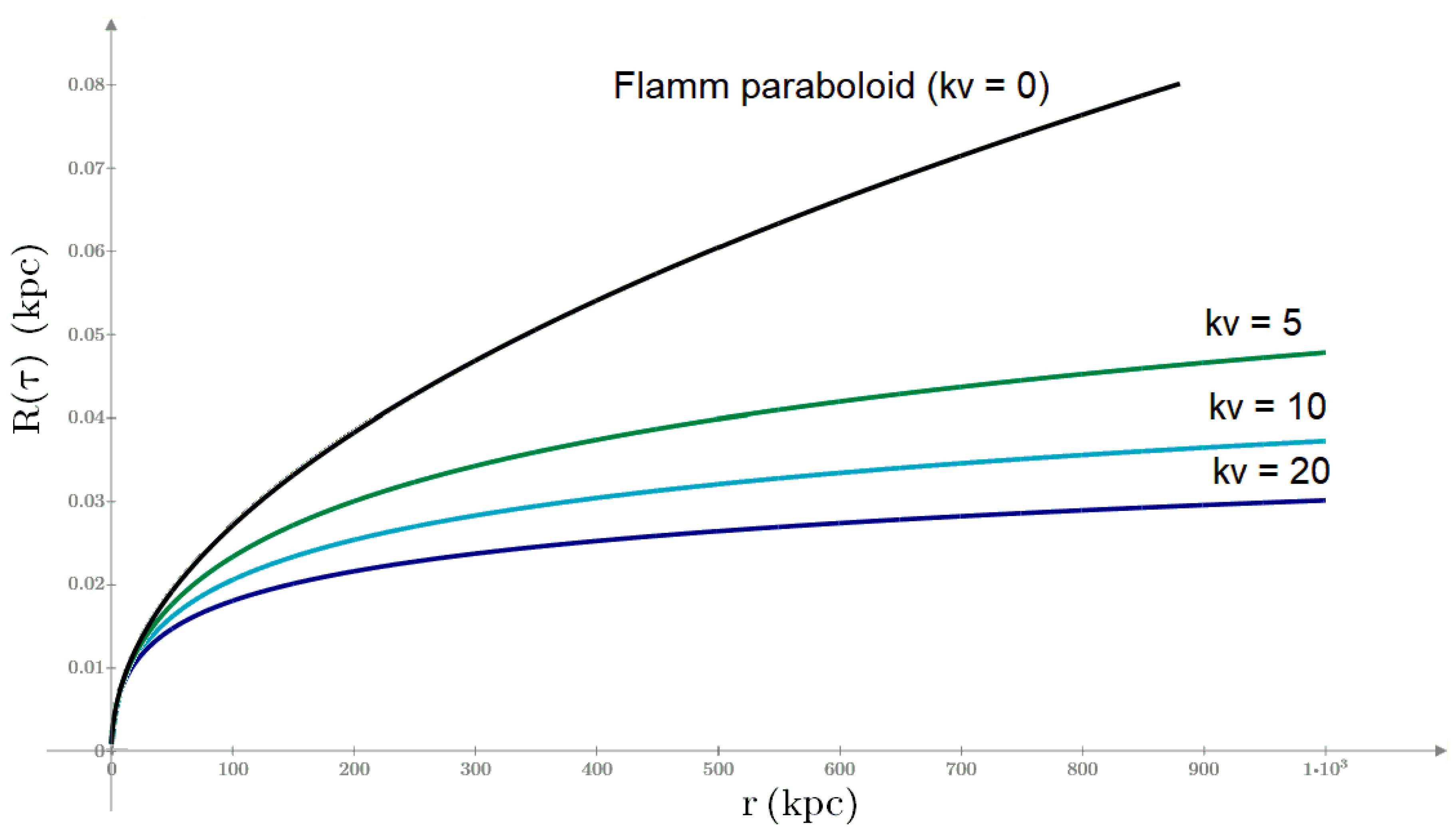
We can now rewrite the slope of the paraboloid as:

$${\displaystyle \frac{dR\left(\tau \right)}{dr}}={\displaystyle \frac{d{R}_U}{dr}}=\sqrt{g_{rr}\left(r\right)-1}=\sqrt{{\displaystyle \frac{R_s{r}_o}{r\left(r+r_o\right)-R_s{r}_o}}}\simeq \sqrt{{\displaystyle \frac{R_s{r}_o}{r\left(r+r_o\right)}}}=\sqrt{{\displaystyle \frac{R_s{R}_v}{r\left(k_v\cdot r+R_v\right)}}}$$

(132)

Integrating with respect to r, we obtain the approximate form of the paraboloid:

$$R\left(\tau \right)=R_U\left(r\right)\simeq -2\sqrt{{\displaystyle \frac{Rs{R}_v}{k_v}}}\ln ({\displaystyle \frac{\sqrt{k_{v}r+R_v}-\sqrt{k_{v}r}}{\sqrt{k_v{R}_s+R_v}-\sqrt{k_v{R}_s}}})$$

(133)

This allows us to graph (next figure) the shape of the paraboloid and see how it changes with different values of k_v.

The expression for the projected cosmological acceleration becomes:

$$g_r\left(r\right)=g_c\left(\tau \right){\displaystyle \frac{\mathrm{d}{R}_u}{\mathrm{d}r}}={\displaystyle \frac{-G{M}_U}{R_U^2}}\sqrt{{\displaystyle \frac{R_s{r}_o}{r(r+r_o)-R_s{r}_o}}}={\displaystyle \frac{-G{M}_U}{R_U^2}}\sqrt{{\displaystyle \frac{R_s{R}_v}{r(k_{v}r+R_v)-R_s{R}_v}}}$$

(134)

We can now introduce this into equation (99) to compute the cosmological velocity:

$$v_C^2\left(r\right)={\displaystyle \frac{-G\cdot M_U\cdot r}{R_U^2}}\sqrt{{\displaystyle \frac{R_s{r}_o}{r\left(r+r_o\right)-R_s{r}_o}}}=g_C\left(\tau \right)\cdot \sqrt{{\displaystyle \frac{r^2{R}_s{R}_v}{r\left(k_{v}r+R_v\right)-R_s{R}_v}}}$$

(135)

Taking the square root again gives:

$$v_C\left(r\right)=\sqrt{g_C\left(\tau \right)}\cdot \sqrt[4]{{\displaystyle \frac{r^2{R}_s{R}_v}{r\left(k_{v}r+R_v\right)-R_s{R}_v}}}$$

(136)

For r >> R_s, we can approximate this as:

$$v_C\left(r\right)=\sqrt{g_C\left(\tau \right)}\cdot \sqrt[4]{{\displaystyle \frac{r{R}_s{R}_v}{k_{v}r+R_v}}}$$

(137)

And in the limit r·k_v >> R_v, this tends toward a constant value:

$$v_C\left(r\right)=\sqrt{g_C\left(\tau \right)}\cdot \sqrt[4]{{\displaystyle \frac{R_s{R}_v}{k_v}}}$$

(138)

Thus, the dependence on r^1/4 that appeared in equation (101) is effectively eliminated.

Therefore, to conclude this section, and assuming—as is commonly done—that the temporal and radial components of the metric satisfy the condition g_tt = c²/g_rr, the new modified Schwarzschild-like metric takes the form:

$$d{s}^2=(1-{\displaystyle \frac{R_s}{r}}\cdot {\displaystyle \frac{R_v}{k_{v}r+R_v}})c^{2}d{t}^2-{\displaystyle \frac{d{r}^2}{1-\frac{R_s}{r}\cdot \frac{R_v}{k_{v}r+R_v}}}-r^{2}d{\Omega }^2-2g_C\left(\tau \right)\sqrt{{\displaystyle \frac{R_s{R}_v}{r\left(k_v\cdot r+R_v\right)}}}drdt$$

(139)

This expression encapsulates the proposed deformation of the Schwarzschild geometry due to the projected cosmological acceleration. The additional cross term g_tr encodes the influence of the 5D cosmological dynamics on the 4D spacetime structure. The presence of the function f(r)=Rv/(kvr+Rv) effectively flattens the Flamm paraboloid at large distances, allowing for the smooth embedding of local Schwarzschild vacuoles within the globally curved 3-sphere geometry of the universe.

To complete the derivation, we now reintroduce the terms that were previously neglected, and revert the time substitution dt =dτ, obtaining::

$$d{s}^2=(1-{\displaystyle \frac{R_s}{r}}\cdot {\displaystyle \frac{R_v}{k_{v}r+R_v}})c^{2}d{\tau }^2-({\displaystyle \frac{1}{1-\frac{r^2}{R_U^2\left(\tau \right)}}}+{\displaystyle \frac{1}{1-\frac{R_s}{r}\cdot \frac{R_v}{k_{v}r+R_v}}}-1)d{r}^2-r^{2}d{\Omega }^2-2\dot{R}\left(\tau \right)\sqrt{{\displaystyle \frac{R_s{R}_v}{r\left(k_v\cdot r+R_v\right)-R_s{R}_v}}}\cdot drd\tau$$

(140)

Finally, we express the metric in terms of the coordinate time by using equation (68), where R_sU is the Schwarzschild radius of the universe (given by equation (55)), and by substituting the expression for $\dot{R}\left(t\right)$ from equation (58), we arrive at the general form of the metric:

$$d{s}^2=(1-{\displaystyle \frac{R_s}{r}}\cdot {\displaystyle \frac{R_v}{k_{v}r+R_v}}){\displaystyle \frac{R_U\left(t\right)}{R_{sU}}}{c}^{2}d{t}^2-({\displaystyle \frac{1}{1-\frac{r^2}{R_U^2\left(t\right)}}}+{\displaystyle \frac{1}{1-\frac{R_s}{r}\cdot \frac{R_v}{k_{v}r+R_v}}}-1)d{r}^2-r^{2}d{\Omega }^2-2c\sqrt{(1-{\displaystyle \frac{R_U\left(t\right)}{R_{sU}}}){\displaystyle \frac{R_s{R}_v}{r\left(k_v\cdot r+R_v\right)-R_s{R}_v}}}\cdot drdt$$

(141)

Equation (141) represents one of the central results of this work: a generalized metric that consistently merges local gravitational fields with the global cosmological evolution dictated by the expansion of the hyperspherical radius R_U(t). Unlike standard Schwarzschild or FLRW metrics—which separately describe local and global structures—this expression provides a unified spacetime geometry incorporating both contributions in a fully geometric and covariant framework.

Structurally, this metric can be seen as a natural analogue to the McVittie metric, which was originally formulated to embed a central mass within an expanding cosmological background. However, in the present model, the coupling between local mass distributions and global dynamics arises not from an ansatz or continuity condition, but from a consistent projection of the 5D cosmological geometry onto the 4D spacetime through the Flamm paraboloid’s deformation and the time evolution of R_U(t). The presence of the cross term g_tr is not postulated, but instead derived as a geometric consequence of the embedding structure.

This formulation confirms and justifies the effective acceleration term g_C previously introduced on heuristic grounds. It also allows for a more rigorous treatment of the rotational dynamics of galaxies, the Tully–Fisher relation, and the cosmological redshift, all within the same metric foundation. Furthermore, the metric reduces to known cases in the appropriate limits: the Schwarzschild geometry is recovered for R_U(t)→const, and a modified FLRW form emerges in the weak-field regime or at cosmological scales where local mass terms become negligible.

As such, equation (141) constitutes the foundational spacetime structure from which the model’s dynamical and observational predictions can be coherently derived.

4.4.2. Modification of the Newtonian Acceleration

In this section, we analyze how the modified form of the Schwarzschild metric, given by equation (139), affects the expression for gravitational acceleration. Specifically, we compute the Newtonian radial acceleration using the g_tt(r) component of the metric. A minus sign is introduced to indicate that the gravitational force is attractive, i.e., directed toward the origin of coordinates:

$$g_N\left(r\right)=-{\displaystyle \frac{1}{2}}{\partial }_r{g}_{tt}$$

(142)

This leads to the expression:

$$g_N\left(r\right)=-{\displaystyle \frac{GM}{r^2}}\left(1-{\left({\displaystyle \frac{k_{v}r}{k_{v}r+R_v}}\right)}^2\right)$$

(143)

As a result, the gravitational acceleration is no longer determined solely by the local mass, but is modified by the influence of the global geometry—specifically, the coupling between the local paraboloid structure and the curvature of the higher-dimensional hypersphere.

4.4.3. Emergent Negative Mass and Its Effect

According to Birkhoff’s theorem, the only spherically symmetric solution to Einstein’s field equations in vacuum is the Schwarzschild metric. Therefore, since we have modified its g_rr(r) component, it is clear that the new metric is no longer a vacuum solution, and mass-energy densities must appear when solving the Einstein equations. Moreover, because the new g_rr(r) component flattens or reduces the slope of the Flamm paraboloid, it is logical to assume that such an effect requires the presence of negative mass density, which, as seen in the previous section, affects the gravitational component.

Starting once again from the modified metric introduced in equation (139), we now solve Einstein’s field equations (3), obtaining the following expression for the G_t^t component of the Einstein tensor:

$$G_t^t=-{\displaystyle \frac{\left(g_C^2\right(\tau )+1)R_v{R}_s{k}_v{r}^2-g_C^2\left(\tau \right)\left(g_C^2\right(\tau )+1)R_v^2{R}_s^2}{r^2(k_v^2{r}^4+R_v{k}_v{r}^3+(2g_C^2\left(\tau \right)R_{v}Rs{k}_v+R_v^2)r^2+2g_C^2(\tau )R_v^2{R}_s^{2}r+g_C^4(\tau \left)R_v^2{R}_s^2\right)}}$$

(144)

In this expression, we can neglect the terms proportional to R_s², since they are significantly smaller. This leads to the simplified form:

$$G_t^t=-{\displaystyle \frac{\left(g_C^2\right(\tau )+1)R_v{R}_s{k}_v{r}^2}{r^2(k_v^2{r}^4+2R_v{k}_v{r}^3+(2g_C^2\left(\tau \right)R_v{R}_s{k}_v+R_v^2\left)r^2\right)}}$$

(145)

If we now further assume that g_C²(τ)+1 ≈ 1 in the numerator, and approximate the denominator by taking 2g_C²(τ)R_vR_sk_v +R_v² ≈ R_v², we finally obtain:

$$G_t^t\simeq -{\displaystyle \frac{k_v\cdot R_v\cdot R_s}{r^2(k_{v}r+R_v{)}^2}}=T_t^t={\displaystyle \frac{8\pi G}{c^2}}\rho \left(r\right)$$

(146)

which yields a negative mass density:

$$\rho \left(r\right)=-{\displaystyle \frac{k_v\cdot R_v\cdot R_s}{r^2(k_{v}r+R_v{)}^2}}\cdot {\displaystyle \frac{c^2}{8\pi G}}$$

(147)

We can now compute the total mass enclosed within a radius r′ using the expression:

$$M\left(r^{\prime }\right)={\int }_0^{r^{\prime }}4\pi r^2\rho \left(r\right)dr={\int }_0^{r^{\prime }}4\pi r^2{\displaystyle \frac{-k_v\cdot R_v\cdot R_s}{r^2(k_{v}r+R_v{)}^2}}{\displaystyle \frac{c^2}{8\pi G}}dr$$

(148)

which gives:

$$M\left(r^{\prime }\right)=-{\displaystyle \frac{c^2{R}_S}{2G}}\cdot {\displaystyle \frac{k_{v}r}{k_{v}r+R_v}}$$

(149)

If we now substitute the expression for R_s from equation (94), we obtain:

$$M\left(r\right)=-M{\displaystyle \frac{k_{v}r}{k_{v}r+R_v}}$$

(150)

where M is the mass of the central object that generates the gravitational field. Thus, this modification of the g_rr(r) component of the original metric results in a negative mass M(r), which subtracts from the positive mass M of the source, reducing the net gravitational mass and, consequently, the gravitational acceleration.

The emergence of a “negative mass density” (Equation 147) as a consequence of modifying the metric component g_rr(r) should not be interpreted as the existence of intrinsically negative mass in the universe. Rather, this term represents a screening effect or an effective reduction of the gravitational influence of baryonic mass at large distances. In this model, the negative mass acts to decrease the slope of the Flamm paraboloid, which is equivalent to a reduction in the net perceived gravity, thereby allowing for the explanation of galactic rotation curves without requiring additional dark matter. It is important to emphasize that, under this interpretation, the net mass density at any point in space remains positive. This “negative mass effect” is a manifestation of the modified geometry of local spacetime, and its deeper study could provide new insights into gravitational interactions in a higher-dimensional context.

At this point, we aim to provide physical meaning and assign values to the parameters k_v and R_v. To do this, we propose identifying R_v with the vacuole radius used in the Einstein–Straus model [2], defined as the comoving radius (in FLRW coordinates) of a sphere that encloses a mass M_g, such that the mass enclosed in that sphere in a homogeneous FLRW universe exactly matches the mass of the object (galaxy, cluster, etc.) represented by the Schwarzschild metric. That is:

$$M_g={\displaystyle \frac{4}{3}}\pi R_v^3{\rho }_u$$

(151)

Where M_g is the mass of the central object (e.g., a galaxy), ρ_U is the average density of the FLRW universe at that cosmological epoch, and R_v is the comoving radius of the vacuole.

Solving for R_v, we obtain

$$R_v=\sqrt[3]{{\displaystyle \frac{M_g}{M_U}}}\cdot R_U$$

(152)

where R_U is the size (radius) of the universe at the corresponding cosmological time.

Once R_v has been identified with the Einstein–Straus vacuole radius, we can compute the negative mass M(R_v) enclosed within that radius using equation (126):

$$\mathrm{M}\left({\mathrm{R}}_{\mathrm{v}}\right)=-{\mathrm{M}}_{\mathrm{g}}{\displaystyle \frac{{\mathrm{k}}_{\mathrm{v}}{\mathrm{R}}_{\mathrm{v}}}{{\mathrm{k}}_{\mathrm{v}}{\mathrm{R}}_{\mathrm{v}}+{\mathrm{R}}_{\mathrm{v}}}}=-{\mathrm{M}}_{\mathrm{g}}{\displaystyle \frac{{\mathrm{k}}_{\mathrm{v}}}{{\mathrm{k}}_{\mathrm{v}}+1}}<-{\mathrm{M}}_{\mathrm{g}}$$

(153)

which is always less than −M_g, with equality only in the limit k_v → ∞.

From this expression, we conclude that the parameter k_v governs the reduction of the Flamm paraboloid slope (as shown in Figure 8) by controlling the amount of negative mass −M(r) enclosed within the radius R_v. A higher value of k_v results in a shallower paraboloid slope and a greater amount of negative mass within R_v.

4.4.4. Derivation of the Mass–Velocity Relation

Previously, in equation (103), we found that M_g ∝ v⁴, in full agreement with the Tully–Fisher relation. In this section, we will examine whether the inclusion of R_v — defined as the vacuole radius — and thus its dependence on M_g, modifies this proportionality relation. Let us analyze this:

If we raise equation (134), which gives v_C(r) for r >> R_v, to the fourth power, we obtain:

$$v_C^4\left(r\right)=g_C^2\left(\tau \right)\cdot {\displaystyle \frac{R_s{R}_v}{k_v}}$$

(154)

Using the definition of R_v from equation (152), we have:

$$v_C^4\left(r\right)=g_C^2\left(\tau \right){\displaystyle \frac{R_s}{k_v}}\cdot \sqrt[3]{{\displaystyle \frac{Mg}{M_U}}}\cdot R_U$$

(155)

Now, substituting the expression for R_s from equation (94), we obtain:

$$v_C^4\left(r\right)=g_C^2\left(\mathsf{\tau }\right){\displaystyle \frac{2G{M}_g}{c^2}}\sqrt[3]{{\displaystyle \frac{M_g}{M_U}}}\cdot {\displaystyle \frac{R_U}{k_v}}=g_C^2\left(\mathsf{\tau }\right){\displaystyle \frac{2G}{c^2}}\sqrt[3]{{\displaystyle \frac{M_g^4}{M_U}}}\cdot {\displaystyle \frac{R_U}{k_v}}$$

(156)

With a bit of algebra, we can isolate the mass of the galaxy and obtain:

$${\mathrm{M}}_{\mathrm{g}}\left(\mathrm{v}\right)={\displaystyle \frac{c\cdot R_U^2}{G^2\cdot M_U}}\sqrt[4]{{\displaystyle \frac{R_U\cdot c^2\cdot k_v^3}{8\cdot G\cdot M_U}}}\cdot v_c^3$$

(157)

That is:

$${\mathrm{M}}_{\mathrm{g}}\left(\mathrm{v}\right)={\displaystyle \frac{c\cdot a_G}{G}}\cdot v_c^3$$

(158)

where

$$a_G={\displaystyle \frac{R_U^2}{G\cdot M_U}}\sqrt[4]{{\displaystyle \frac{R_U\cdot c^2\cdot k_v^3}{8\cdot G\cdot M_U}}}$$

(159)

In summary, from equation (133) we obtain the following relation:

$$M_g\left(v\right)\propto v_c^3$$

(160)

This expression differs from the classical Tully–Fisher relation M ∝ v⁴. In addition to the change in the exponent of v_c, the new expression (157) has no dependence on the radial distance, unlike equation (102), which included a 1/r dependence.

4.5. Derivation of MOND from Cosmological Acceleration

The hypothesis proposed in this work—that a portion of the cosmological acceleration g_C(τ) in the extra dimension R is projected onto our three-dimensional universe, generating an effective acceleration g_r(r), which in turn leads to a constant radial velocity at large distances as given by equation (154), similarly to MOND [3] enables us to explore a possible theoretical justification for the empirical MOND parameter a₀.

In the limit of large radial distances r, the previously derived expression for g_r(r) can be approximated as:

$$g_r\left(r\right)={\displaystyle \frac{-G{M}_U}{R_U^2}}\sqrt{{\displaystyle \frac{R_s{R}_v}{r\left(k_{v}r+R_v\right)-R_s{R}_v}}}\simeq {\displaystyle \frac{-G{M}_U}{R_U^2}}\sqrt{{\displaystyle \frac{R_s{R}_v}{k_v}}}\cdot {\displaystyle \frac{1}{r}}$$

(161)

On the other hand, MOND assumes that, in the very low acceleration regime, where g << a₀:

$$a_r\left(r\right)=\sqrt{G{M}_g{a}_0}\cdot {\displaystyle \frac{1}{r}}$$

(162)

Equating both expressions, we obtain:

$$\sqrt{a_{0}G{M}_g}={\displaystyle \frac{G{M}_U}{R_U^2}}\sqrt{{\displaystyle \frac{R_s{R}_v}{k_v}}}={\displaystyle \frac{G{M}_U}{R_U^2}}\sqrt{{\displaystyle \frac{2G{M}_g}{c^2{k}_v}}\cdot \sqrt[3]{{\displaystyle \frac{M_g}{M_U}}}{R}_U}$$

(163)

This allows us to isolate the MOND parameter a₀:

$$a_0={\left({\displaystyle \frac{G{M}_U}{R_U^2}}\right)}^2{\displaystyle \frac{2}{c^2{k}_v}}\cdot \sqrt[3]{{\displaystyle \frac{M_g}{M_U}}}{R}_U={\left({\displaystyle \frac{G{M}_U}{c}}\right)}^2\cdot {\displaystyle \frac{2}{k_v{R}_U}}\cdot \sqrt[3]{{\displaystyle \frac{M_g}{M_U}}}$$

(164)

which implies

$${\mathrm{a}}_0\propto \sqrt[3]{{\mathrm{M}}_{\mathrm{g}}}$$

(165)

This result is noteworthy, as some extended MOND models and emergent gravity theories have also suggested a dependence of a₀ on galaxy mass. In our model, this relation emerges naturally from the 5D spacetime geometry and the projection of the cosmological acceleration.

Finally, expression (164) enables us to estimate the value of the total mass of the universe M_U. Assuming the standard MOND value a₀ = 1.2·10^-10 m/s², and taking k_v = 15 (the value that best fits galaxy rotation curves, as will be shown later), we find that for a typical range of galactic masses M_g∈[1,100]·10⁹ M_⊙, the estimated total mass of the universe is:

$${\mathrm{M}}_{\mathrm{U}}\simeq \left[0.5-4\right]\cdot {10}^{60}\hspace{0.17em}\mathrm{k}\mathrm{g}$$

(166)

This value is several orders of magnitude higher than the standard estimate in the ΛCDM framework (M_U ≃1.53·10 ⁵³ kg), but it is consistent with the predictions of our 5D model, as discussed in the section on galactic rotation curves and subsequent analyses.

4.6. Application to Galaxy Rotation Velocity Curves

In this section, we aim to apply the newly obtained expressions for g_N(r) and g_r(r), in order to assess whether galaxy rotation curves can be explained without resorting to dark matter.

If we write the condition for centripetal balance for an object of mass m rotating in a circular orbit at distance r from a central mass M, which generates the gravitational field, we have:

$$\mathrm{m}{\displaystyle \frac{v^2\left(r\right)}{r}}=\mathrm{m}\cdot g_N\left(\mathrm{r}\right)+\mathrm{m}\cdot g_r\left(r\right)$$

(167)

where g_N(r) is the gravitational acceleration as given by equation (143), and g_r(r) is the cosmological acceleration given by equation (134), so that:

$$v_t^2\left(r\right)=\left(g_N\right(r)+g_r(\tau \left)\right)\cdot r={\displaystyle \frac{G{M}_g}{r}}(1-({\displaystyle \frac{k_{v}r}{k_{v}r+R_v}}{)}^2)+{\displaystyle \frac{G{M}_U}{R_U^2}}\cdot \sqrt{{\displaystyle \frac{r^2{R}_s{R}_v}{r(k_{v}r+R_v)-R_s{R}_v}}}$$

(168)

For r > > Rs, this can be approximated by:

$$v_t^2\left(r\right)={\displaystyle \frac{G{M}_G}{r}}(1-({\displaystyle \frac{k_{v}r}{k_{v}r+R_v}}{)}^2)+{\displaystyle \frac{G{M}_U}{R_U^2}}\cdot \sqrt{{\displaystyle \frac{r{R}_s{R}_v}{(k_{v}r+R_v)}}}$$

(169)

Taking the square root yields:

$$v_t\left(r\right)=\sqrt{{\displaystyle \frac{G{M}_g}{r}}(1-({\displaystyle \frac{k_{v}r}{k_{v}r+R_v}}{)}^2)+{\displaystyle \frac{G{M}_U}{R_U^2}}\cdot \sqrt{{\displaystyle \frac{2GMg{R}_{v}r}{c^2(k_{v}r+R_v)}}}}$$

(170)

We can define v_N(r) and v_C(r) such that:

$$v_t\left(r\right)=\sqrt{v_N^2\left(r\right)+v_C^2\left(r\right)}$$

(171)

where:

$$v_N\left(r\right)=\sqrt{{\displaystyle \frac{G{M}_g}{r}}\left(1-{\left({\displaystyle \frac{k_{v}r}{k_{v}r+R_v}}\right)}^2\right)}$$

(172)

and

$$v_C\left(r\right)={\displaystyle \frac{G{M}_U}{R_U^2}}\cdot \sqrt[4]{{\displaystyle \frac{2G{M}_g{R}_{v}r}{c^2(k_{v}r+R_v)}}}$$

(173)

Before checking whether equation (170) fits the observed galaxy rotation curves, we must make one more adjustment. In the previous equations, the entire mass M_g of the galaxy was assumed to be concentrated at its center, which leads to an overly steep velocity profile at small r. To correct this, we assume a mass distribution within the galaxy of the form:

$$M_{g_0}\left(\mathrm{r}\right)=M_o\cdot {\displaystyle \frac{r^2}{r^2+r_o^2}}$$

(174)

Alternatively, for galaxies where the central mass increases less abruptly, we may use:

$$M_{g_1}\left(\mathrm{r}\right)=M_o\cdot {\left({\displaystyle \frac{r^2}{r^2+r_1^2}}\right)}^2$$

(175)

These mass distribution functions are proposed forms and may be replaced by others. Additionally, while other studies often include contributions from radiation and gas, in this work we assume that these effects are already accounted for in the chosen mass profiles.

To obtain the Newtonian velocity corresponding to the mass distribution M_g(r), we apply Gauss’s theorem and find:

$$v_N\left(r\right)=\sqrt{{\displaystyle \frac{G{M}_g\left(r\right)}{r}}\left(1-{\left({\displaystyle \frac{k_{v}r}{k_{v}r+R_v}}\right)}^2\right)}$$

(176)

and the cosmological speed as:

$$v_C\left(r\right)={\displaystyle \frac{G{M}_U}{R_U^2}}\cdot \sqrt[4]{{\displaystyle \frac{2G{M}_g\left(r\right)R_{v}r}{c^2(k_{v}r+R_v)}}}$$

(177)

Then, the total velocity of a star at distance r is given by:

$$v_t\left(r\right)=\sqrt{v_N^2\left(r\right)+v_C^2\left(r\right)}=\sqrt{{\displaystyle \frac{G{M}_g\left(r\right)}{r}}\left(1-{\left({\displaystyle \frac{k_{v}r}{k_{v}r+R_v}}\right)}^2\right)+{\displaystyle \frac{G{M}_U}{R_U^2}}\cdot \sqrt{{\displaystyle \frac{2G{M}_g\left(r\right)R_{v}r}{c^2\left(k_{v}r+R_v\right)}}}}$$

(178)

Here, v_N(r) is the Newtonian term, and v_C(r) the new term arising from cosmological acceleration.

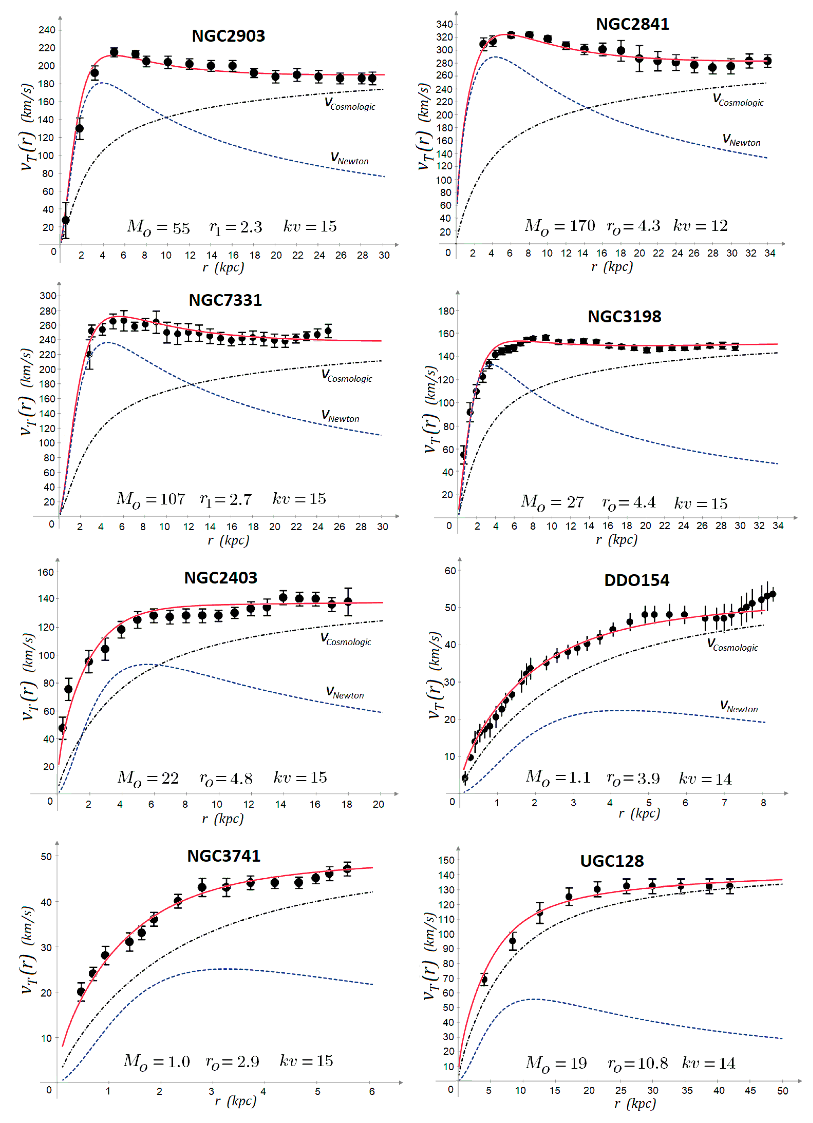
Now that we have equation (178), we can test its ability to reproduce observed galaxy rotation curves. Data from eight galaxies of varying sizes, masses, and rotation speeds were used to fit equation (154) by adjusting relevant parameters.

Among the parameters to adjust are the cosmological ones: the total mass M_U and current radius R(τ) of the universe, which depends on the Hubble parameter via equation (86). These values must remain fixed for all galaxies. For each galaxy, we then fit the specific values of the galactic mass M₀ and the scale radius r₀ or r₁, depending on the chosen profile.

A first attempt using the standard values M_U = 1.53·10⁵³ kg and R(τ) = 1.212·10²⁶ m, as obtained in equation (90), results in negligible values of v_C(r). After manual tuning, the value of M_U that best fits all eight galaxies is:

$${\mathrm{M}}_{\mathrm{U}}=3.0\cdot {10}^{60}\hspace{0.17em}\mathrm{k}\mathrm{g}$$

(179)

This value lies within the range [0.5 – 4] ·10⁶⁰ kg previously obtained in equation (166).

This would imply a maximum Schwarzschild radius for the universe of:

$$R_S=4.45\cdot {10}^{33}\hspace{0.17em}m=4.71\cdot {10}^{17}\hspace{0.17em}light-years$$

(180)

Solving equation (86), we obtain the current size of the universe:

$$\mathrm{R}\left(\mathsf{\tau }\right)=4.25\cdot {10}^{28}\hspace{0.17em}\mathrm{m}=4.50\cdot {10}^{12}\hspace{0.17em}\mathrm{l}\mathrm{i}\mathrm{g}\mathrm{h}\mathrm{t}-\mathrm{y}\mathrm{e}\mathrm{a}\mathrm{r}\mathrm{s}$$

(181)

Using equation (63), the current cosmological (coordinate) time is:

$$\mathrm{t}=4.50\cdot {10}^{12}\hspace{0.17em}\mathrm{y}\mathrm{e}\mathrm{a}\mathrm{r}\mathrm{s}$$

(182)

And from equation (78), the proper time is:

$$\tau =9.27\cdot {10}^9\hspace{0.17em}years$$

(183)

Although the estimated age of the universe in proper time (τ ≈ 9.27×10⁹ years) and the total mass of the universe (M_U ≈ 3.0×10⁶⁰ kg) differ significantly from the values adopted in the ΛCDM model, it is plausible that the shorter age predicted by this model could still be reconciled with the observed formation of cosmic structures. One hypothesis worth exploring is that the stronger cosmological acceleration during the early stages of the universe—an intrinsic feature of the present model—might have enhanced the rate of galaxy and structure formation, allowing the observable universe to reach its current state in a shorter period of time. This is a line of research that would require detailed investigation in future work.

To conclude this section, the following figures present the rotation velocity curves of eight galaxies. The black dots (with error bars) represent the observed values from [4]. The blue dashed curves show the Newtonian velocity v_N(r), while the black dotted curves correspond to the cosmological velocity v_C(r). The red line is the total velocity v_t(r) obtained from equation (171). Galaxy masses M_o are given in units of 10⁹ M_⊙, and radial distances are expressed in kiloparsecs.

From these plots, it can be concluded that equation (178) fits the observed rotation curves quite well. Therefore, the cosmological acceleration given by equation (134) provides an additional velocity term that allows us to reproduce galactic rotation curves without invoking dark matter.

Figure 9. Rotation curves for different galaxies including cosmological velocity.

Figure 9. Rotation curves for different galaxies including cosmological velocity.

4.7. Wide Binary Systems

Wide binary systems are composed of two stars with masses on the order of one solar mass, whose dynamics are studied at distances of up to 200 astronomical units (au). The goal is to determine whether the relative acceleration between the stars follows the classical Newtonian behavior, or whether it agrees with the predictions of modified gravity theories such as MOND. This range of distances and masses has been chosen because it leads to accelerations on the order of the MOND characteristic constant, a₀ = 1.2×10⁻¹⁰ m/s².

It has been observed that, in this regime, wide binary systems exhibit dynamics consistent with Newtonian gravity and not with MOND [5]. This is often interpreted as a significant challenge for MOND, which predicts deviations from Newtonian behavior in this weak-acceleration regime.

In this section, we apply the model proposed in this work, which introduces a cosmological acceleration projected onto 3D space, derived in previous sections. We analyze whether this additional term significantly affects the dynamics of these systems or, on the contrary, whether Newtonian behavior is preserved.

To do this, we compare the expressions for the Newtonian acceleration g_N(r) and the projected cosmological acceleration g_r(r), given by equations (143) and (134), respectively. Taking stellar masses on the order of 1 M_⊙, the associated vacuole radius is:

$$R_v=\sqrt[3]{{\displaystyle \frac{Mg}{M_U}}}\cdot R_U=2.48\cdot {10}^7\hspace{0.17em}au$$

(184)

This value is much larger than the distance range of interest (up to 200 au). In this regime, the Newtonian acceleration simplifies to:

$${\mathrm{g}}_{\mathrm{N}}\left(\mathrm{r}\right)=-{\displaystyle \frac{\mathrm{G}{\mathrm{M}}_{\mathrm{g}}}{{\mathrm{r}}^2}}\left(1-{\left({\displaystyle \frac{{\mathrm{k}}_{\mathrm{v}}\mathrm{r}}{{\mathrm{k}}_{\mathrm{v}}\mathrm{r}+{\mathrm{R}}_{\mathrm{v}}}}\right)}^2\right)\simeq -{\displaystyle \frac{\mathrm{G}{\mathrm{M}}_{\mathrm{g}}}{{\mathrm{r}}^2}}$$

(185)

Thus, the classical Newtonian form is recovered.

Regarding the cosmological acceleration, from equation (134), for r < < R_v, we can approximate:

$$g_r\left(r\right)={\displaystyle \frac{-G{M}_U}{R_U^2}}\sqrt{{\displaystyle \frac{R_s{R}_v}{r(k_{v}r+R_v)-R_s{R}_v}}}\simeq {\displaystyle \frac{-G{M}_U}{R_U^2}}\sqrt{{\displaystyle \frac{R_s{R}_v}{r(k_{v}r+R_v)}}}\simeq {\displaystyle \frac{-G{M}_U}{R_U^2}}\sqrt{{\displaystyle \frac{R_s}{r}}}$$

(186)

where R_s is the Schwarzschild radius of the system. Substituting the expression for R_s, we obtain:

$$g_r\left(r\right)\simeq {\displaystyle \frac{-G{M}_U}{R_U^2}}\sqrt{{\displaystyle \frac{2G{M}_g}{c^2\cdot r}}}$$

(187)

By equating g_r(r) with g_N(r), we find the value of r at which both accelerations are equal:

$$\mathrm{r}=\sqrt[3]{{\displaystyle \frac{{\mathrm{M}}_{\mathrm{g}}\cdot {\mathrm{R}}_{\mathrm{U}}^4\cdot {\mathrm{c}}^2}{2\cdot \mathrm{G}\cdot {\mathrm{M}}_{\mathrm{U}}^2}}}\simeq 5.3\cdot {10}^5\hspace{0.17em}\mathrm{a}\mathrm{u}$$

(188)

This value is significantly greater than the typical 200 au scale of wide binary systems. Consequently, we conclude that within the range of distances considered, the dynamics of these systems remain purely Newtonian, in perfect agreement with observations. This prediction of the model sets it apart from MOND and reinforces its validity in low-acceleration regimes.

4.8. Velocity Dispersion in Galaxy Clusters: A 5D Virial-like Relation Without Dark Matter

From equation (157), we have previously found that mass is proportional to the cube of velocity, that is, M ∝ v³. This leads us to postulate that the relationship between mass and the velocity dispersion σ_v in galaxy clusters should also follow the form:

$$M=A_{\sigma }\cdot {\sigma }_v^3$$

(189)

where A_σ is a proportionality constant.

This expression allows us, given a pair of values (M, σ_v), to determine A_σ, and using that value, check whether the observational data can be fitted accordingly. To this end, we use the following plot obtained from [6], which shows the velocity dispersion as a function of mass for different models such as MOND and Newton + dark matter (DM).

Figure 10. Predictions of velocity dispersion from several models.

Figure 10. Predictions of velocity dispersion from several models.

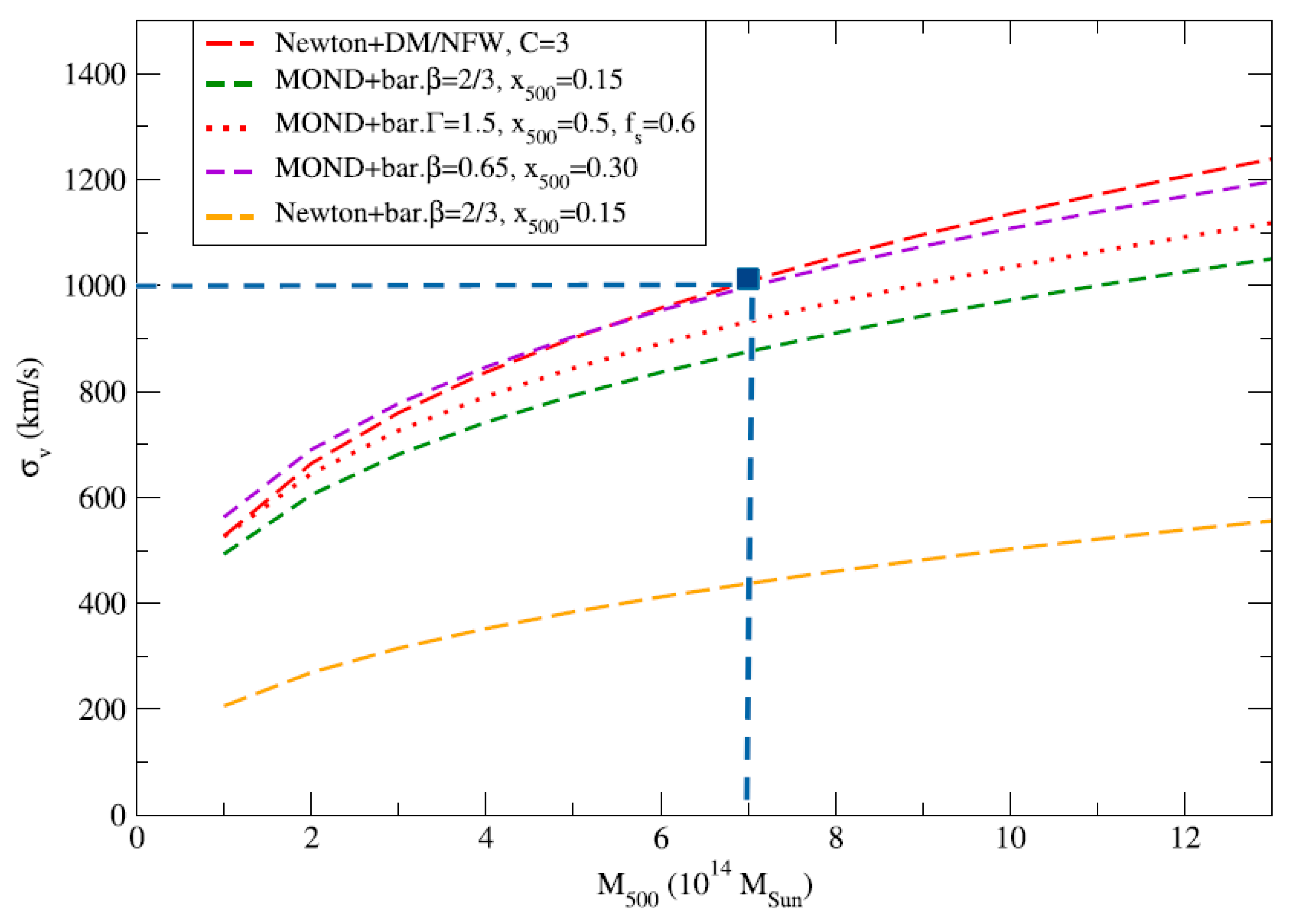
In the above figure, the masses along the X-axis, denoted M₅₀₀, are considered total masses in the Newton + DM case. For the MOND models, the baryonic mass is computed using the relation:

$$M_{bar.500}=0.117\cdot 10^{14}({\displaystyle \frac{M_{500}}{10^{14}{M}_{\odot }}}{)}^{1.16}{M}_{\odot }$$

(190)

In our case, we assume the baryonic mass corresponds to 15% of the total mass:

$$M_{bar.500}=0.15\cdot M_{500}\cdot {10}^{14}\cdot M_{\odot }$$

(191)

If we choose the point (7, 1000) in the graph, then the values used to calibrate A_σ become (0.15·7, 1000) = (1.05, 1000), which gives:

$$A_{\sigma }={\displaystyle \frac{M_{bar.500}}{{\sigma }^3}}={\displaystyle \frac{1.05\cdot {10}^{14}\cdot M_{\odot }}{{\left(1000km/s\right)}^3}}=105000{\displaystyle \frac{M_{\odot }}{{\left(km/s\right)}^3}}$$

(192)

Thus, the general expression for our model becomes:

$$M_{bar.500}=105000{\displaystyle \frac{M_{\odot }}{(km/s{)}^3}}\cdot {\sigma }_v^3$$

(193)

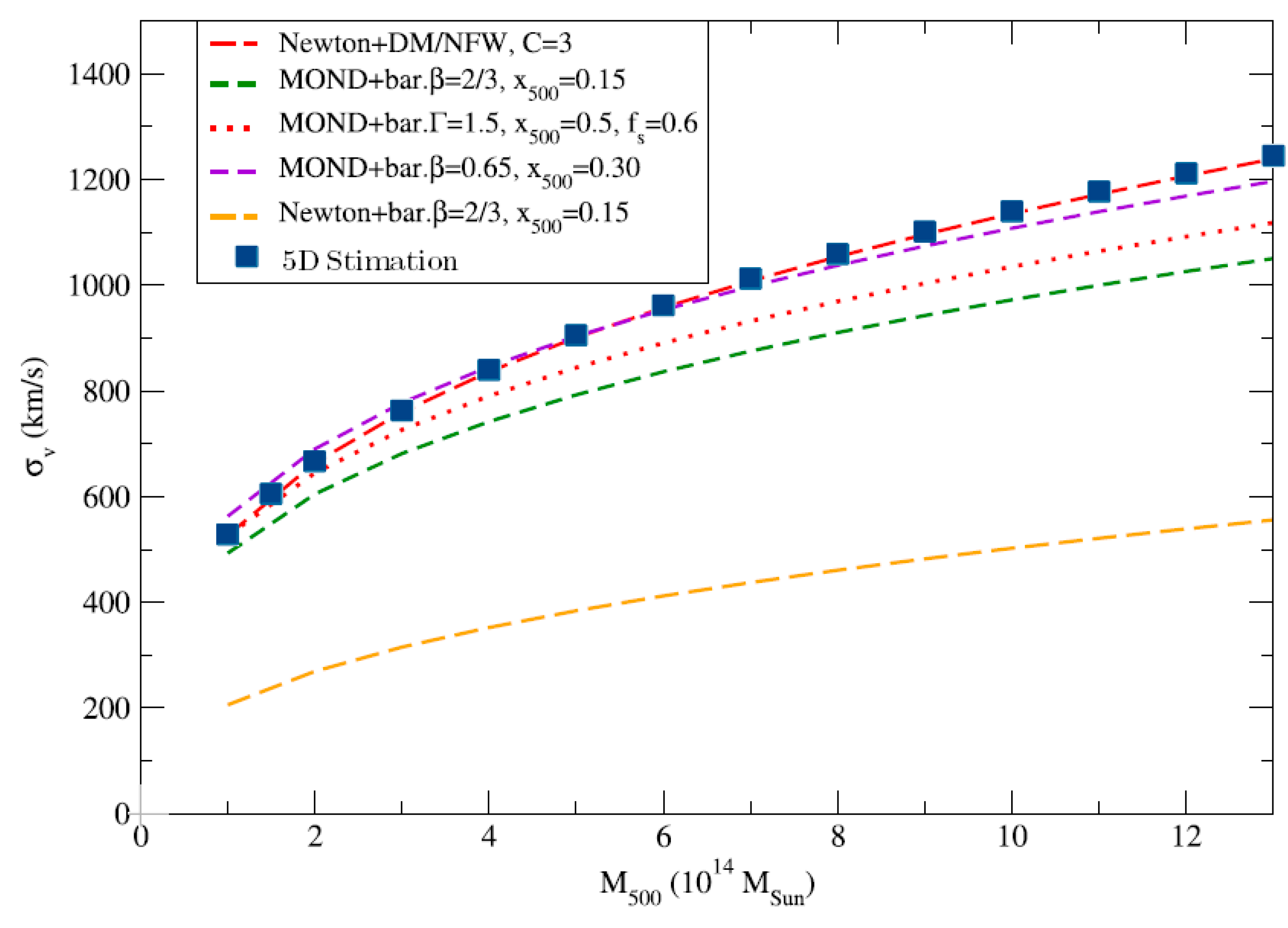
We now use this expression to test whether it correctly fits the data shown in the figure. The result is displayed in the following figure, where the blue squares represent predictions using equation (193) within the 5D model. As can be observed, the expression aligns very well with the red curve corresponding to the Newton + DM/NFW model.

Figure 11. Predictions of the velocity dispersions for the 5D model.

Figure 11. Predictions of the velocity dispersions for the 5D model.

The final step is to check whether the value of A_σ, previously obtained by fitting, can be derived directly from the 5D velocity equation. To do this, we assume a proportional relationship between velocity and velocity dispersion of the form:

$$v=C\cdot {\sigma }_v$$

(194)

where v is the velocity given by equation (157). Therefore, the following must hold:

$$M_g\left(v\right)={\displaystyle \frac{c\cdot R_U^2}{G^2\cdot M_U}}\sqrt[4]{{\displaystyle \frac{R_U\cdot c^2\cdot k_v^3}{8\cdot G\cdot M_U}}}\cdot v^3={\displaystyle \frac{c\cdot R_U^2}{G^2\cdot M_U}}\sqrt[4]{{\displaystyle \frac{R_U\cdot c^2\cdot k_v^3}{8\cdot G\cdot M_U}}}\cdot {\left(C\cdot {\sigma }_v\right)}^3$$

(195)

Comparing with equation (193), we obtain:

$${\displaystyle \frac{c\cdot R_U^2}{G^2\cdot M_U}}\sqrt[4]{{\displaystyle \frac{R_U\cdot c^2\cdot k_v^3}{8\cdot G\cdot M_U}}}\cdot C^3=A_{\sigma }=105000{\displaystyle \frac{M_{\odot }}{\mathrm{k}{\mathrm{m}}^3/{\mathrm{s}}^3}}$$

(196)

Using k_v = 15 (similar to the value used in the study of galaxy rotation curves), and substituting all known values, we find:

$$v=2.58\cdot {\sigma }_v$$

(197)

While it is usually considered that for self-gravitating systems:

$$v=\sqrt{3}\cdot {\sigma }_v\simeq 1.73\cdot {\sigma }_v$$

(198)

obtaining the correct value of A_σ in equation (196) by simply taking C = 2.58 can be regarded as a success of the 5D model, demonstrating a precise match between the theoretical framework and the empirical fit.

We can therefore conclude that the 5D geometrical model presented in this work, through its M ∝ v³ relation, is capable of explaining velocity dispersion in galaxy clusters using only the baryonic mass, without requiring the presence of dark matter.

4.9. Dark Energy and the Accelerated Expansion of the Universe

In the previous section, we applied the concept of cosmological acceleration and its effects to various observational results, demonstrating that they can be successfully explained without the need to introduce dark matter. However, for all the above to hold significance, it is essential that such cosmological acceleration does indeed exist and is negative —that is, that the universe is undergoing decelerated expansion.

Therefore, now it is necessary to give a satisfactory explanation compatible with the above to the results and measurements that seem to indicate that the universe, contrary to what is obtained in this text, is not expanding accelerately but is doing so decelerately, that is, more and more slowly.

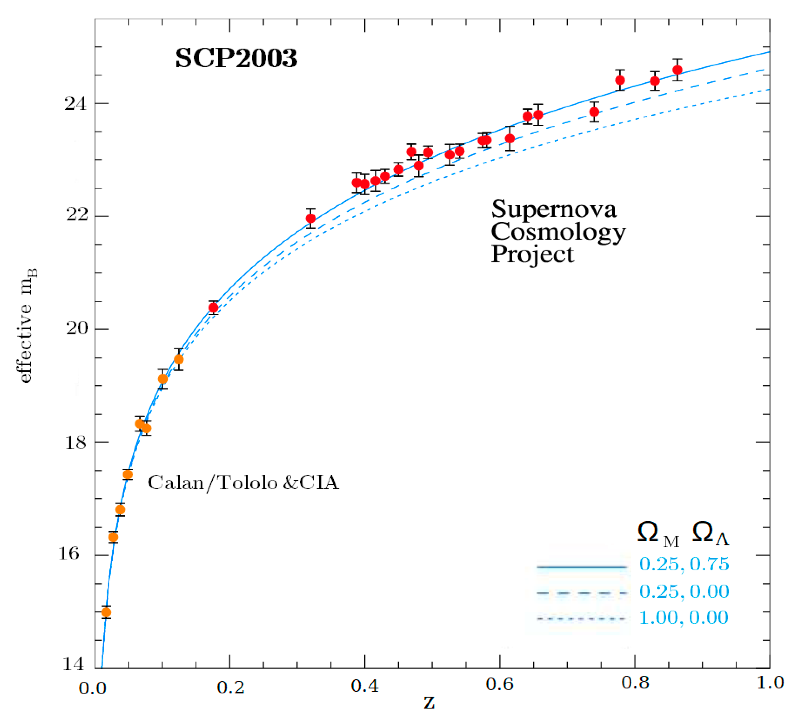
The figure below shows the Hubble diagram obtained by the Supernova Cosmology Project in 2003 [7] showing the effective value of M_B based on redshift z, where we can assume that it is defined as:

$$m_B^{effective}=5\cdot log\left(D_L\left(z,{\Omega }_M,{\Omega }_{Lambda}\right)\right)+25$$

(199)

with D_L being the distance of light, which can be considered to have the expression:

$$D_L\left(z\right)=r{R}_o\left(1+z\right)$$

(200)

where r is the comoving radial coordinate.

The value of D_L indicated by (200) has been obtained by assuming that:

$$1+z_{expansion}={\displaystyle \frac{{\nu }_1}{{\nu }_2}}={\displaystyle \frac{d{t}_2}{d{t}_1}}={\displaystyle \frac{{\lambda }_2}{{\lambda }_1}}={\displaystyle \frac{R_2}{R_1}}=1+z$$

(201)

where ν₁ and λ₁ are the frequency and wavelength of the emitted radiation, and where ν₂ and λ₂ indicates the current observed value. The above equalities can be obtained in different ways through the FLRW metric.

At this point, it is time to recover the expression of the metric obtained in (67):

$$\mathrm{d}{s}^2={\displaystyle \frac{R\left(ct\right)}{R_S}}{c}^2\mathrm{d}{t}^2-R^2\left(ct\right)\left({\displaystyle \frac{\mathrm{d}{r}^2}{1-r^2}}+r^2\mathrm{d}{\theta }^2+r^{2}si{n}^2\theta \mathrm{d}{\varphi }^2\right)$$

(67)

This form, in which g_tt = R/Rs ≠ 1, implies the existence of an additional gravitational redshift between comoving observers located at different values of the cosmic radius R. In general relativity, gravitational redshift occurs because clocks run at different rates depending on the gravitational potential. Between two observers at R₁ and R₂, the gravitational redshift is given by:

$$1+z_{grav}=\sqrt{{\displaystyle \frac{g_{tt}\left(R_2\right)}{g_{tt}\left(R_1\right)}}}=\sqrt{{\displaystyle \frac{R_2/R_S}{R1/R_S}}}=\sqrt{{\displaystyle \frac{R_2}{R1}}}$$

(202)

Therefore, the total redshift between the emission and observation events, assuming both effects combine multiplicatively, is:

$$1+z_{total}=(1+z_{grav})\cdot (1+z_{expansion})=\sqrt{{\displaystyle \frac{R_2}{R_1}}}\cdot {\displaystyle \frac{R_2}{R_1}}=({\displaystyle \frac{R_2}{R_1}}{)}^{3/2}$$

(203)

This result leads to a total time dilation of:

$${\displaystyle \frac{d{t}_2}{d{t}_1}}={\displaystyle \frac{{\upsilon }_1}{{\upsilon }_2}}=({\displaystyle \frac{R_2}{R_1}}{)}^{3/2}=(1+z{)}^{3/2}$$

(204)

Now, using the above ratio, it can be deduced that the distance of light given by (200) will be modified by taking into account the temporal dilation, obtaining that:

$$D_{Ld}\left(z\right)=r{R}_o{\left(1+z\right)}^{3/2}=D_L\left(z\right)\sqrt{1+z}$$

(205)

being D_L(z) the distance of light obtained in (200) without taking into account the time dilation.

Figure 12. Hubble diagram obtained by the Supernova Cosmology Project in 2003.

Figure 12. Hubble diagram obtained by the Supernova Cosmology Project in 2003.

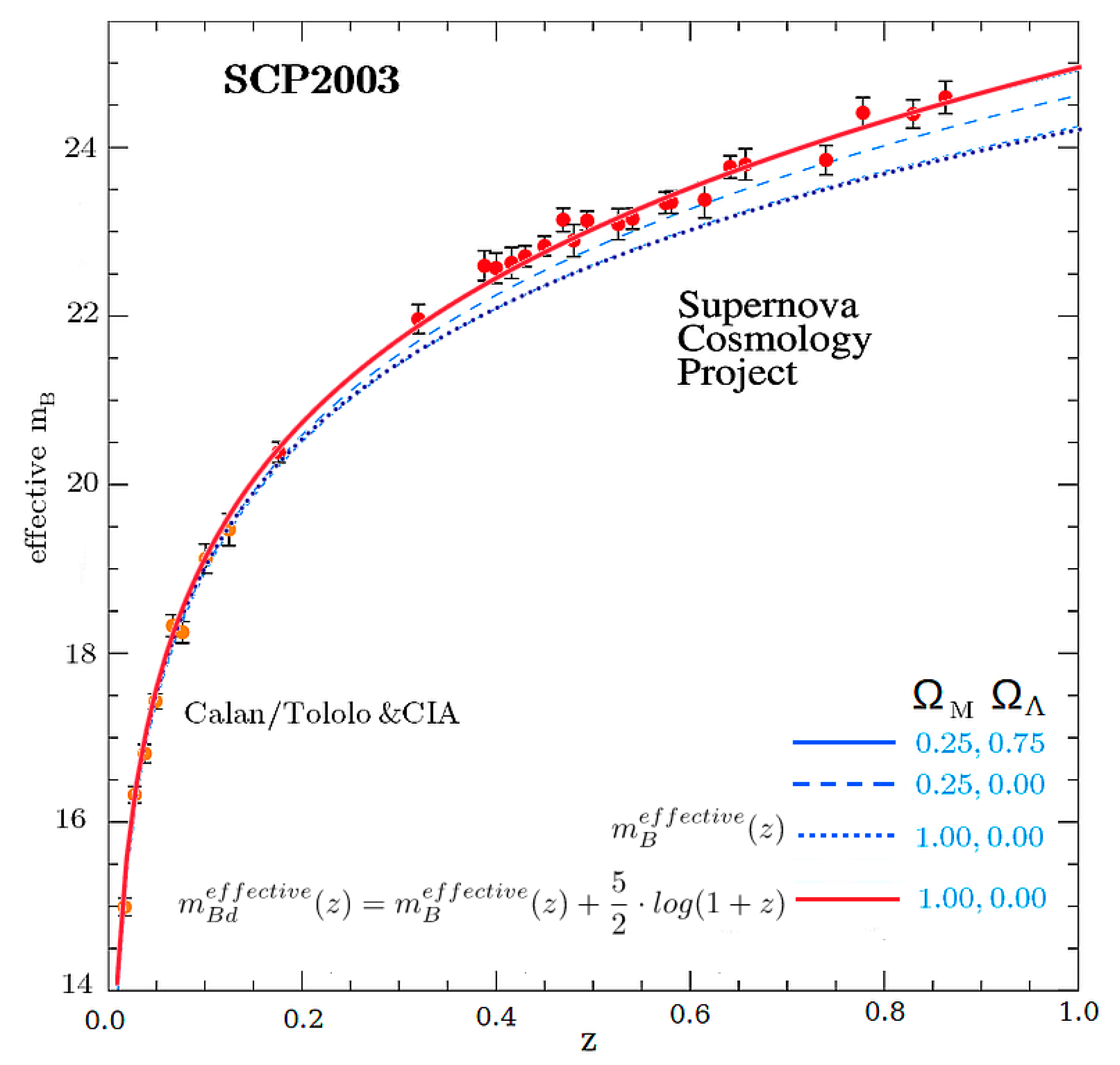
Therefore, if we now use the previous expression in (199) we will obtain that the effective value of m_Bd^effective(z) if gravitational redshift is taken into account, it will be:

$$m_{Bd}^{effective}\left(z\right)=5\cdot log\left(D_{Ld}\left(z\right)\right)+25=5\cdot log\left(D_L\left(z\right)\sqrt{1+z}\right)+25$$

(206)

and if we continue to operate, we get that:

$$m_{Bd}^{effective}\left(z\right)=5\cdot log\left(D_L\left(z\right)\right)+{\displaystyle \frac{5}{2}}\cdot log\left(1+z\right)+25$$

(207)

Therefore, the effective value of m_Bd^effective(z) will be:

$$m_{Bd}^{effective}\left(z\right)=m_B^{effective}\left(z\right)+{\displaystyle \frac{5}{2}}\cdot log\left(1+z\right)$$

(208)

If we now represent graphically (red line) the previous expression taking as m_B^effective(z) the theoretical values for a universe composed only of cold matter (i.e. Ω_M = 1.0 and Ω_Λ = 0.0) and superimpose it on the Hubble diagram obtained by the Supernova Cosmology Project, we will see that the values of m_Bd^effective(z) obtained with the expression (208) coincides perfectly with those obtained for a universe with dark matter and dark energy with densities Ω_M = 0.25 and Ω_Λ = 0.75 respectively.

Thus, by incorporating both the standard cosmological redshift (201) and the gravitational redshift (202), and combining them to obtain the total redshift (203), we recover (208), which provides an accurate fit to the observational data without invoking dark energy. This result supports the conclusion that the universe is indeed undergoing decelerated expansion, consistent with the theoretical predictions of this 5D model.

Figure 13. In red, the mBdeffective(z) values superimposed on the Hubble diagram of the Supernova Cosmology Project.

Figure 13. In red, the mBdeffective(z) values superimposed on the Hubble diagram of the Supernova Cosmology Project.

5. Universe Dominated by Dark Energy

At this point in the paper, it would be normal to end this study by analyzing a universe dominated solely by dark energy. But since we have shown in the Section 4.9 that it is not necessary to introduce it to explain the Hubble diagrams of supernovae, we believe that we can affirm the non-existence of such dark energy and, therefore, we will ignore this study and end here the analysis of the different models of universes.

6. Conclusions

This work is based on the hypothesis that the universe is confined to the surface of a three-dimensional hypersphere embedded in a higher-dimensional space. Within this framework, we have proposed a new metric in which the hyperspherical radius R(t) evolves with cosmological time. The resulting four-dimensional spacetime is formally analogous to the FLRW metric, with the scale factor a(t) replaced by R(t). While the spatial part retains the standard structure, the temporal component introduces a gravitational redshift through the modified form of g_tt.

Applying Einstein’s field equations to this metric leads to a new set of Friedmann-like equations, which yield, without the need for additional assumptions, the correct pressure–density relations for both radiation and matter. This ensures compatibility with the standard cosmological evolution and highlights the internal consistency of the proposed geometric framework.

In both radiation- and matter-dominated regimes, the equations predict a decelerated expansion of the universe driven by the gravitational pull of its total mass-energy content. While such deceleration is also predicted by the standard FLRW model without a cosmological constant, the novelty of this proposal lies in the hypothesis that the global deceleration—rooted in the higher-dimensional geometry—can project an additional acceleration onto the observable 3D universe. This mechanism provides a natural explanation for the flat rotation curves of galaxies and the velocity dispersion observed in galaxy clusters, without invoking non-baryonic dark matter. Furthermore, the model predicts a mass–velocity relation of the form M∝ v³, as opposed to the classical Tully–Fisher relation M∝ v⁴.

The model has also been applied to wide binary systems, yielding purely Newtonian dynamics—unlike MOND-type theories, which typically fail to reproduce observations in such systems. Interestingly, the MOND acceleration scale a₀ can be derived within this framework, showing that it scales with the cube root of the mass, a₀ ∝ M^1/3, in agreement with certain extended MOND formulations.

Finally, the new metric reproduces the Hubble diagram obtained by the Supernova Cosmology Project without the need for dark energy. The observed accelerated expansion of the universe is instead interpreted as a relativistic illusion caused by time dilation effects associated with the expansion velocity in the extra dimension R. In this view, the universe is not accelerating but rather decelerating under its own gravity, as expected in a matter-dominated scenario.

In summary, if the statements and derivations presented in this paper are correct, one may conclude that our universe lies on the surface of a four-dimensional hypersphere expanding within a higher-dimensional space. Its radius is currently increasing at extremely high velocities. While the coordinate expansion speed approaches 99.999% of the speed of light as seen from an external reference frame, for a comoving observer within the hyperspherical universe the expansion speed is much greater—on the order of 324 c—according to equation (74). This hyperluminal expansion, which cannot be reconciled with the standard framework of Special Relativity, supports the need for generic transformations as discussed in [8].

The expansion is being decelerated by the gravitational pull of the universe’s own mass and is expected to reach a maximum radius R_S, at which point it will halt and begin to contract. Remarkably, this critical radius exactly matches the Schwarzschild radius corresponding to the universe’s total mass M_U. This suggests that, from a higher-dimensional perspective, our observable universe may reside within the interior of a five-dimensional black hole, with the expanding 3-sphere hypersurface lying inside its event horizon.

6.1. Comparison with Other Models

For clarity and completeness, the following table summarizes how each of the main gravitational models—Newtonian gravity, Newtonian gravity with dark matter, MOND, and the present 5D hyperspherical model—addresses the key phenomena discussed throughout this paper.

Phenomenon / Model	Newtonian Gravity	Newton + Dark Matter	MOND	5D Hyperspherical Model
Wide binary systems	✅ Yes	✅ Yes	❌ No	✅ Yes
Galactic rotation curves	❌ No	✅ Yes	✅ Yes	✅ Yes
Velocity dispersion in clusters	❌ Too low	✅ Yes	❌ Too low	✅ Yes
Accelerated expansion	❌ Not explained	❌ Needs dark energy	❌ Not explained	✅ Explained via time dilation
Tully-Fisher relation	❌ Not predicted	✅ Predicted (with tuning)	✅ Predicted (as input)	✅ Derived: M ∝v3

6.2. Simplicity and Key Parameters of the Model

One of the most compelling features of the proposed 5D geometric framework is its structural simplicity. Despite its predictive power across multiple astrophysical phenomena—galactic rotation curves, wide binary dynamics, cluster velocity dispersions, and cosmological expansion—it relies on a very limited set of physical parameters. No free functions or fitted empirical laws have been introduced beyond the geometry itself and well-defined cosmological constants. In contrast with other models requiring dark components or additional postulates, the present model leverages only the curvature of a higher-dimensional hyperspherical space and its projection into the observable 3D universe. This simplicity strengthens the internal coherence and the explanatory scope of the theory.

To highlight the internal consistency and simplicity of the model, we present in the follow table, the key parameters used in the 5D formulation, along with their definitions and numerical estimates, where applicable.

Symbol	Description	Estimated Value	Units
MU	Total mass of the universe	3.0 x 1060	kg
RU	Radius of the hypersphere (today)	4.25 × 1028 4.50 x 1012	m light-years
Rs	Maximum Radius of the hypersphere	4.45 × 1033 4.71 x 1017	m light-years
ρU	Density of the universe (today)	9.31 x 10-27 (slightly above the critical density of ΛCDM)	kg/m3
t	Coordinate time (global evolution)	4.50 × 1012	years
τ	Proper time (comoving observer)	9.27 × 109	years
kv	Slope control parameter for the Flamm paraboloid	12–16 (depending on galaxy)	–
gc(τ)	Cosmological acceleration (today)	1.11 x 10-7	m/s2
Aσ	Constant of proportionality between mass and velocity dispersion (Eq. (165))	105000	M⊙/km3s3

7. Discussions

This work introduces a geometric model offering a promising alternative to the dark matter and dark energy paradigms. A natural next step will be to explore the broader implications of replacing dark components with gravitational redshift effects and cosmological acceleration, as derived from higher-dimensional geometry, across various epochs of the universe.

A particularly promising line of inquiry lies in the mass-velocity relation predicted by our model. While the classical Tully-Fisher relation is based on M∝v⁴, our theoretical framework naturally leads to an M∝v³ scaling. This difference arises as a direct consequence of the projection of the universe’s decelerating expansion onto the local dynamics of galaxies. This finding presents a clear opportunity to revisit existing and future observational data, assessing whether the empirical Tully-Fisher law might require adjustment or reinterpretation under this new theoretical perspective.

Furthermore, it’s crucial to emphasize that our model not only reproduces the flattening of galactic rotation curves without invoking dark matter but also predicts that this flattening could persist out to distances as large as 1 to 2 megaparsecs. This constitutes a clear, quantifiable, and testable prediction; it would be of great interest to examine whether current or forthcoming observations support the presence of extended flat rotation curves beyond typical galactic scales.

If the hypotheses developed in this paper prove correct, they could provide strong support for Einstein’s General Relativity, reinforcing the idea that phenomena currently attributed to dark components might instead arise as relativistic manifestations within a curved higher-dimensional spacetime. In this scenario, alternative theories of gravity, such as MOND or scalar-tensor models, may lose their appeal or necessity.

Finally, a fundamental outcome of this work is the successful construction of a generalized metric, formally analogous to the McVittie metric. This new metric incorporates both local Schwarzschild-like gravitational potentials and the global evolution of the hyperspherical radius R(t). It allows for a coherent and covariant embedding of local gravitational systems within a dynamic cosmological background, maintaining full consistency with the geometric and dynamic features discussed. Future research should continue to explore the mathematical properties of this generalized spacetime, including its energy-momentum tensor, geodesic structure, and causal boundaries, to further solidify the foundations of this higher-dimensional cosmological model.

8. Relation with Previous Works

This paper constitutes a substantially revised and extended version of a prior preprint published on Qeios [9]. While the core geometric hypothesis remains the same, the present version includes a full derivation of the projected cosmological acceleration from the metric, a generalized Schwarzschild-like metric embedded in a hyperspherical background, and an expanded discussion of observational implications.

References

- Tully, R.B.; Fisher, J.R. A New Method of Determining Distances to Galaxies. Astronomy and Astrophysics. 1977, 54, 661–673. [Google Scholar]
- Einstein, A. Straus, E. G. The influence of the expansion of space on the gravitation fields surrounding the individual stars. Reviews of Modern Physics 1945, 17, 120–124. [Google Scholar]
- Milgrom, M. A modification of the Newtonian dynamics as a possible alternative to the hidden mass hypothesis. Astrophysical Journal 1983, 270, 365–370. [Google Scholar] [CrossRef]
- Marr, John. Galaxy rotation curves with log-normal density distribution. Monthly Notices of the Royal Astronomical Society 2015, 448. [CrossRef]
- Pittordis, C.; Sutherland, W. Wide binaries as a critical test of classical gravity: confronting Gaia DR3 with MOND predictions. Monthly Notices of the Royal Astronomical Society 2023, 519, 3937–3956. [Google Scholar]
- M López-Corredoira, J E Betancort-Rijo, R Scarpa, Ž Chrobáková, Virial theorem in clusters of galaxies with MOND, Monthly Notices of the Royal Astronomical Society. 2022; 517, 5743. [CrossRef]
- R.A. Knop et al. New Constraints on ΩM, ΩΛ, and w from an Independent Set of 11 High-Redshift Supernovae Observed with the Hubble Space Telescope. The Astrophysical Journal 2003, 598, 102–137. [CrossRef]
- José Gabriel Ramírez Escalona. Is the Special Relativity Compatible With Einstein’s Static Universe?Proposal for New “Generic” Transformations. The Twin Paradox. Qeios. 2024. [CrossRef]
- José Gabriel Ramírez Escalona. Cosmology in Five Dimensions: Is Our Universe the Surface of a Four-Dimensional Hypersphere? Application to Dark Matter and Dark Energy. Qeios 2024. [CrossRef]
Figure 8.
Flamm’s Paraboloide in function of kv.
Disclaimer/Publisher’s Note: The statements, opinions and data contained in all publications are solely those of the individual author(s) and contributor(s) and not of MDPI and/or the editor(s). MDPI and/or the editor(s) disclaim responsibility for any injury to people or property resulting from any ideas, methods, instructions or products referred to in the content. |
© 2025 by the authors. Licensee MDPI, Basel, Switzerland. This article is an open access article distributed under the terms and conditions of the Creative Commons Attribution (CC BY) license (http://creativecommons.org/licenses/by/4.0/).
Copyright: This open access article is published under a Creative Commons CC BY 4.0 license, which permit the free download, distribution, and reuse, provided that the author and preprint are cited in any reuse.