
Submitted:
16 August 2024
Posted:
27 August 2024
You are already at the latest version
Abstract
We investigate the cosmological evolution of the universe for a spatially flat FLRW background space within the context of $f(T,B)$ gravity, which is a recently formulated teleparallel theory that connects both $f(T)$ and $f(R)$ gravity under suitable limits. The analysis has been done by focusing on four different $f(T,B)$ cosmological models corresponding to various choices of scale factor, namely emergent, logamediate, and intermediate. In addition to this, we also assume a power-law-like function of $f(T,B)$ gravity. The reconstruction of $f(T,B)$ gravity has been done by considering the Holographic Ricci Dark Energy(HRDE) (a particular case of a highly generalized holographic dark energy given in Nojiri et al. in General Relativity and Gravitation, 38, pp.1285-1304,2006) as the background fluid. We analyze the equation of state parameters and the squared speed of sound for the reconstructed models. Finally, we conducted the thermodynamical analysis for each reconstructed model. The generalised second law of thermodynamics(GSLT) is valid for the four different $f(T,B)$ cosmological models.
Keywords:
Holographic Ricci Dark Energy
; $f(T
; B)$ gravity
; scale factor
1. Introduction
The current cosmology scenario is teeming with a plethora of models that aim to explain what is perhaps simultaneously the most exciting and confounding phenomenon observed in the past few decades, the late-time acceleration [1,2,3,4]. It was first discovered in the year 1998 when observations of SNeIa collated by the high-redshift SN team [5] and SN cosmology project [6] appeared as illuminating candles idicating that the universe’s expansion was accelerating. Ever since, increasing observational evidence [7,8] have only affirmed the accelerated expanding paradigm of the Universe. These measurements and observations have resulted in the introduction of a new mysterious energy component known as dark energy [9,10,11,12,13,14] which is attributed with a negative pressure. Over the years, robust efforts have been made to understand the accelerated phenomenon. For this purpose researchers have proposed various dark energy models such as the cosmological constant [15,16] which is considered to be the simplest model phenomenologically and is known as CDM [17] model when the cold dark matter constitutes the standard cosmological model. Models without the cosmological constant include scalar fields [18], tachyon fields [19], Chaplygin gas [20,21], bouncing models [22,23], braneworld models [24,25,26] and so on. These models have been studied in the framework of General Relativity(GR) [27] where the space-time is mediated by by curvature. However, the interest in modified [28,29,30,31] and extended theories of gravity [32,33,34] have been increasingly attracting the attention of cosmologists in recent years as it seems to be a promising alternative to GR in providing a systematic and geometric explanation of numerous cosmological phenomena. One can find in [35] an extensive review of modified gravities that are looked into as gravitational alternatives for dark energy. The authors have shown the rich cosmological structure within the realms of modified gravity that could naturally lead to an effective cosmological constant, quintessence or phantom era in the late universe with the possibility of a transition from deceleration to acceleration or the crossing of the phantom divide, if necessary, due to the gravitational terms which increase with the scalar curvature decrease. In addition, they have demonstrated that some of the discussed models in their work could possibly pass the Solar System tests.
In the modified theory, also known as f theories, Einstein-Hilbert action [36] of GR given by where R is the Ricci scalar, is the gravitational coupling constant and is the determinant of the metric tensor, is replaced by a more general action and the gravity theory [37,38,39] is considered to be the simplest f theory. In this approach, an arbitrary function of the Ricci scalar is introduced and the Einstein-Hilbert action is recovered when is a linear function. Comparisons with observational data in the case of theory have been studied in [40,41,42,43,44]. An important work in the context of a unified description of the inflationary era with the dark energy within the modified gravity framework was done by [45]. In their work, they have provided the latest developments in modified gravity and have aimed to provide a virtual "toolbox" containing all the necessary information on inflation, dark energy and bouncing solutions in the context of various forms of modified gravity. Other proposed modified gravity models include gravity( is the trace of energy-momentum tensor ) [46,47], gravity() [48], scalar-tensor theories [49,50,51] etc. In [52], the authors have discussed the structure and cosmological properties of various modified theories including theories, scalar-tensor theoriy, Gauss-Bonnet theory, non-local gravity, non-minimally coupled models, Horava-Lifshitz gravity etc. The paper is focused on the possible unification of early-time inflation with late-time acceleration within such theories while assuming a spatially flat FRW cosmology. It was demonstrated that the qualitative possibility of such a unification is a very natural property for the discussed alternative gravities.
In addition to this, another important alternative theory of gravitation in terms of torsion has been introduced that is known as the teleparallel equivalent of General relativity(TEGR) [53,54,55]. It was first proposed by Einstein and in this theory the Levi-Civita Connection is substituted by a so-called Weitzenbock connection [56]. Thus, while GR is based on the Reimannian geometric foundations, teleparallel theory of gravity is based on the work by Weitzenbock and others who laid the foundations for a torsional rather than curvature-based formulation of gravity. Extensive research done in the recent years on torsional gravity, namely gravity, can be found in [57,58,59,60,61,62]. We mention here that the local Lorentz invariance breaks down in the case of gravity formulation, which is its major problem. Extended and modified forms of teleparallel gravity have thus been introduced to construct a covariant formulation of gravity. For example, in [63] the new approach includes choosing a non-zero spin connection and pure-gauge. One might also refer to [64] where a more general approach is considered which contains the squares of the irreducible parts of the torsion . Despite the loss of Lorentz invariance, the standard teleparallel approach is still very prevalent among research topics in literature. This arises from the fact that the covariant issue can somehow be "abated"(only at the level of the field equations) by choosing the correct tetrads [65]. We may mention here that in the case of FLRW cosmology, one can always obtain "good tetrads" for the non-trivial cosmological solutions. An additional alluring property correlating GR and TEGR is that the Ricci scalar is equivalent to the sum of the torsion and total divergence term B(boundary term). In this context, one may refer to [66] in which the authors have proposed an interesting model termed as model wherein the the torsion and boundary scalars contribute independently of each other through the arbitrary function f. It may be noted that this theory becomes equivalent to theory for choosing a special form of . It has been shown [67,68] that for teleparallel gravity, CDM models can be reconstructed, and the holographic dark energy models can be described.
While investigating the various cosmological scenarios, one may also consider various revolutionary theories emerging from string theory and black-hole thermodynamics. These startling theories have illuminated some unexpected corners of the nature of space-time and its relation to energy, matter, and entropy, which in turn have had grave implications in cosmology. The holographic principle [69,70,71,72] is an example of a radical change in modern concepts. The principle requires that the degrees of freedom of a spatial region reside on the surface of the region rather than in the interior. Additionally, it states that the number of degrees of freedom per unit area should not be greater than 1 per Planck area. Thus the area of a region in Planck units must not be exceeded by its entropy. Fischler and Susskind [73] first proposed a cosmological version of holographic principle. The holographic Nojiri-Odintsov model [74] is the most general holographic dark energy(HDE) model and all other known HDE models [75,76,77,78,79,80] are particular examples of this model. A holographic approach to describe the early acceleration and the late-time acceleration eras of our universe can be found in [81]. The "holographic unification" has been demonstrated in the context of and gravity theory wherein the IR cut-offs are taken in terms of particle horizon or future horizon and their derivatives. Their work proves how the holographic principle can be very useful to unify the cosmological eras of the universe. Another work that deserves mentioning in the context of such a unification scenario is the study carried on by [82]. In their work, a modified holographic cut-off is proposed which gives a smooth unified cosmological scenario from a constant roll inflation era to the dark-energy era at the late-time of the universe. Inspired by the prevailing ideas on the Holographic dark energy, Gao et. al.[83] proposed the HRDE model in which the IR cut-off in the holographic model is taken to be the average radius of the Ricci scalar curvature i.e . Thus, in this case, the holographic dark energy density is . Highly generalized versions of HDE were presented in [84,85]. One can see [86] for a more detailed description. These studies conclude that the HRDE model works fairly well in explaining observations such as cosmic acceleration, possibly leading us to understand the problem of cosmic coincidence. Section 3 of our work has been dedicated to reconstructing the gravity with the HRDE taken as the background fluid. Therefore, in our work, we have aimed to apply the cosmological reconstruction methods to this theory, assuming the Holographic Ricci dark energy(HRDE) as the background fluid in three different scenarios corresponding to three different forms of scale factor, namely, emergent, intermediate, and logamediate scale factor, and then to study various cosmological properties of this model such as its thermodynamics and the EoS parameter to investigate the late-time acceleration within the context of our model.
There is an established connection between gravitation and thermodynamics, thus one might infer that the connection can be created between the horizon entropy and the area of a black hole. One can find the investigations into the second law of thermodynamics in the context of horizon cosmology in [87]. In particular, they consider different forms of the horizon entropy and for each, they have focused on different cosmological epochs of the universe. [88] have shown such a connection between the FLRW equations and the first law of thermodynamics(FLT) at the apparent horizon for , where is the temperature and is the radius of the apparent horizon. It was shown by [89] that the Friedmann equations in GR can be written as where the work term W is defined as . In addition, their work has been extended to braneworld gravity [90,91], scalar-tensor gravity [92], f (R) gravity [93], and, Lovelock gravity [94]. [95] have determined a general form of entropy that connects Friedmann equations for any gravity theory with the apparent horizon thermodynamics and have carried on to find the respective entropies for several modified theories of gravity. In their work, they have also proposed a modified thermodynamic law of apparent horizon, free from certain difficulties, which proves to be valid for all EOSs of the matter field. In the context of gravity, the generalised first and second laws of thermodynamics were also studied for different forms of the function in [96,97,98]. Here we are interested in studying the generalised second law of thermodynamics for the different reconstructed models corresponding to different scale factors. This has been done both by using and without using the first law.
Our work is thus organised as follows: in Section 2 we briefly introduce the cosmology with all the basic formalisms that are required for the reconstruction of gravity which has been incorporated in Section 3 where in each subsection we have used a different scale factor. The thermodynamical analysis for each reconstructed model obtained have been done in Section 4.
2. Cosmology
Before we delve into the cosmological reconstruction of models, we explore the cosmology that arises from gravity, a fourth-order generalized teleparallel theory of gravity when considering a flat homogeneous and isotropic metric. The FLRW metric, which describes the space-time in Cartesian coordinates, is given by [99]
where a(t) is the scale factor. The choice of tetrad taken is [100]
In this choice, the spin connections are allowed to be zero i.e., [101]. In gravity, the integral of the gravitational action is a function f of the scalar T and of the boundary term B, i.e., [102]
where . We note here that infinite choices for the tetrad satisfy Eqn. (2) yet only a small subset are considered good tetrads, meaning they have a vanishing spin connection. It can be proved that this choice of tetrad shows the second and fourth-order contributions of the torsion scalar T and the boundary term [103]
and
Hence, gravity exists as a subsets of gravity where
This choice of tetrad shows the second and fourth-order contributions of the torsion scalar T and the boundary term B.
Now if the universe is considered to be filled with a perfect fluid and the FLRW tetrad given in (2) is taken, then the field equations for gravity becomes
Here is the Hubble parameter. The dots represent the differentiation with respect to t, represents the derivative of with respect to T. Similarly, denotes the derivative of with respect to B. In addition, and represent the energy density and pressure of the matter content. Equations (7) and (8) can be written in fluid form as:
The given equations above are akin to standard FLRW equations as in GR. Taking , the quantities appearing in the above equations can be written in terms of gravity as follows:
The given basic equations in this section now help us proceed with our model’s reconstruction and thermodynamical analysis.
3. Reconstruction of Gravity
The infrared cutoff of a quantum field theory, which is connected to the vacuum energy, and the maximum distance of this theory are established by the holographic principle, which has its roots in black hole thermodynamics and string theory. In this section, we have endeavored to reconstruct the gravity associated with the flat FLRW cosmology in the background of Holographic Ricci Dark Energy(HRDE). Different scale factors, viz. emergent, intermediate, and logamediate scale factors, have been employed to construct different cosmological models and study the corresponding EoS parameter. The universe is considered to be filled by a holographic fluid whose energy density is given as the holographic Ricci dark energy(HRDE) [104]
In the subsections below, we reconstruct three different cosmological models corresponding to three different types of scale factors within the background of HRDE and study their properties in cosmology like its thermodynamics.
3.1. Emergent Cosmological Model
One can find extensive investigations [105,106,107,108] into the possibilities of an emergent universe that is ever-existing and large enough so that space-time may be treated as classical entities. We may mention here that there is no time-like singularity in these models, so the universe is in an almost static state in the infinite past. Still, it eventually evolves into an inflationary stage. Thus, a model of a perpetually existing universe, which eventually enters into the Big Bang epoch, is of considerable interest to us. A general framework for an emergent universe has been shown in [109]. This section aims to study the EoS for such a universe considering the HRDE as the exotic fluid within the context of gravity.
The emergent scale factor is written as follows [110]
where , , and . Since , we obtain the Hubble parameter as a function of t:
Thus, the energy density of HRDE is obtained by substituting the above equation in Equation (13) as:
In addition, T and B can be obtained from Equations (4) and (5) respectively as:
and
Thus, the derivative of B with respect to t:
Assuming that the function can be written in the following form:
Using Equations (17) and (18), Eqn. (7) becomes:
where K is a constant for the method of separation and and . For the reconstruction of this model, we equate and , which is the energy density of HRDE, in Equation (9) which then changes it to the following form:
Here we have taken and (by using the matter conservation equation). Thus, by making the essential substitutions we have obtained the reconstructed and plotted its behaviour against time as shown in Figure 1.
Next, we use Equation (11) to derive the reconstructed as:
where
the pressure has been obtained by using the following conservation equation with the additional geometric component
Here, i.e the derivative of with respect to T and thus, represents the derivative of with respect to t. These substitutions helped us to derive the reconstructed pressure(). Finally, using the reconstructed pressure and density we obtained the EoS parameter() by substituting the equations in . The graph for the evolution of EoS parameter against time has been shown in Figure 2. Figure 2 shows that for varying choices of and the EoS parameter shows a phantom behaviour and is asymptotically tending to at a later stage.
The nature of dark energy can be investigated through its EoS parameter and the sound speed of perturbations [111] to the dark energy density and pressure. These perturbations can be described mathematically through the sound speed [112]
For our case, the derivative of reconstructed density obtained in Equation (24) and pressure() can be obtained and substituted in Equation (26) to obtain the sound speed for our particular emergent model in gravity. The behaviour of was plotted against time and is shown in Figure 3.
3.2. Intermediate Cosmological Model
The intermediate inflationary model was first described by Barrow [113] in which the scale factor increases at a rate intermediate between that of the power law models[114] and the conventional de-Sitter models [115]. The main assumption in his paper was that the pressure and density were related by the following equation of state
Here, when , the standard equation of state for a perfect fluid, , is obtained. However, it is when and that the intermediate inflationary scenario is created in which the scale factor expands as [116]
and is known as the intermediate scale factor. Here, and are constants. The Universe exhibits slower expansion for standard de Sitter inflation, which occurs when , yet faster than the power-law inflation, , is a constant. These models have many interesting properties, specifically with the perturbation spectra they generate, which have been studied in [117]. Our work uses the above-given scale factor to study the intermediate scenario for gravity. The methodology adopted in this subsection is similar to that applied to the emergent model. Thus, the Hubble parameter is obtained from Equation (27) as
In this case, the energy density of HRDE is obtained as
Once again, T and B have been obtained by employing Equations (4) and (5). Thus,
and
Thus, the derivative of B with respect to t:
To find the specific form of the function , we assume the functional form as given in Eqn. (20). Thus, using Equations (30) and (31), Eqn. (7) becomes:
Similar to the previous model, the reconstructed has been obtained by using Equation (23). Figure 4 shows its behaviour plotted against time.
Using the derivative of with respect to t and making appropriate substitutions in Equation (11) we have reconstructed the energy density for the intermediate scale factor in the cosmology. Thus,
Here,
We note that ExpIntegralE(n,z) gives the exponential integral function .Additionally, and has a branch cut discontinuity in the complex z plane running from 0 to ∞. However, for certain special arguments, ExpIntegralE can evaluate to exact values. In the present case, for the set of arguments we are getting specific values of the function and getting plots for the equations involving . We have then used the reconstructed to obtain the reconstructed pressure() by substituting the energy density in the conservation equation given in Equation (25). The reconstructed EoS parameter thus obtained was plotted against time and has been presented in Figure 5 where it can be seen that the EoS parameter exceeds the phantom boundary() and shows a quintessence behaviour().
3.3. Logamediate Cosmological Model
When weak general conditions [118] are applied to cosmological models, a class of potential indefinite cosmological solutions known as logamediate inflation arises. The existence of eight possible asymptotic solutions for cosmology dynamics was put forth by Barrow [119]. Of these possible solutions, three led to non-inflationary expansions, and three others gave rise to power law, de Sitter and intermediate expansion. The remaining two solutions showed asymptotic expansions of the logamediate form. Additionally, logamediate inflation naturally arises in a few scalar-tensor theories [120]. In the case of logamediate cosmology, the scale factor evolves as [121]
Here, and . The Hubble parameter in this case is:
The energy density of HRDE for this case of logamediate scale factor is given by
Additionally, the torsion scalar and boundary term are derived as
and
The derivative of B with respect to t:
To find the specific form of the function , we assume the functional form as given in Eqn. (20). Thus, using Equations (39) and (40), Eqn. (7) becomes:
Here,
Just as it was done for the intermediate and emergent cosmological models, can be determined from Equation (23) and the graph so obtained has been shown in Figure (Figure 7).
The plot for the EoS parameter was also plotted and shown in Figure 8. From the figure, we observe the crossing of the phantom boundary in the later stages of the universe, thus resulting in a transition from quintessence to phantom, hinting at a possible Big Rip singularity.
3.4. Power Law Model
In this case, we consider a Lagrangian of separated power law style model for the boundary term and the torsion scalar as given in [122]:
Here, k,l,m and n are all constant terms. Thus, the derivative corresponding to and functions for this model are:
Additionally, we have chosen the intermediate scale factor as given in Eqn. (27) as our choice of scale factor in this subsection. The effective density is obtained by substituting Equations (20), (46) and (28) in Eqn. (11). Doing so, we obtained:
where
Similar substitutions have been made in Eqn. 12 to obtain the pressure as:
where
We can also obtain the EoS parameter for this model using Equations (11) and (12) as:
Thus, by making essential substitutions we could obtain the EoS parameter of this model which has been analysed by considering 3 cases (see Figure 9):
- Case 1: varying k and m with
- Case 2: varying k and m with
- Case 3: varying m and n as negative values
From the figures, we notice that with Case 1(cf. with Figure 9-left), there is a transition from quintessence in the early universe to phantom at a later stage while for Case 2(cf. with Figure 9-middle), we see an accelerated expansion phase() for after which the acceleration isn’t preserved until . At the later stages of the universe, the EoS evolves into a phantom phase and the acceleration is preserved. In Case 3(cf. with Figure 9-right), crossing of phantom boundary is observed.
4. Thermodynamics of Gravity
At this point of our study, we intend to explore the validity of the generalised second law(GSL) of thermodynamics [123] using the previously obtained reconstructed energy density() and pressure () in the emergent, intermediate and logamediate scenarios bounded by the apparent horizon(). This has been done both using and without the first law of thermodynamics. We mention here that we are considering a flat() FRW cosmology with the line element as given in Equation (1) and an equilibrium description of thermodynamics, i.e., the internal temperature is the same as that of the apparent horizon. To begin with, we may define the GSL as an implication that the sum of the entropy inside the horizon() and the entropy of the boundary of the horizon always increases against the evolution of time. For our study, we consider the apparent horizon which in terms of the Hubble parameter is written as:
and the derivative with respect to time is obtained as:
We take the Hawking temperature that is associated with the apparent horizon and define through the surface gravity as:
where .
An important equation while studying the validity of GSL is the Gibbs equation [124] which is written, for the entropy within the apparent horizon, as:
where and are the total energy density and pressure respectively that is contributed by matter and dark energy. Since we are considering a non-interacting model consisting of a perfect fluid and pressure-less matter within the realms of modified gravity, the continuity equation is written as:
Here, and . By using the Gibb’s equation given in Equation (52) together with the continuity equation(53), one obtains:
in which is the rate of internal energy change with repect to time. In addition, and . In addition, the quantities and are the reconstructed pressure and density obtained in the previous section for the different scale factors. We will now find the expression for the total entropy change using the first law and without using the first law of thermodynamics.
4.1. GSL Using First Law
In the representation of the field equations of gravity as given in Equations (2) and (3), the derivative of the apparent horizon() with respect to time is given as:
The Berkenstein-hawking horizon entropy in the context of general relativity is given by [125]
Here, and G is the Newton constant. Bahamonde et. al. [126] has used the above relation together with the Misner-Sharp energy given by:
and obtained the following:
where and . Thus, they proved that it is possible for the traditional first law of thermodynamics to be met while considering the equilibrium thermodynamic description of gravity. We may note that heat flow through the horizon is just the amount of energy crossing it during the time interval . Thus, the first law of thermodynamics(Clausus relation) on the horizon can be written as . We can use the unified first law to then obtain
From the equation given above, we get the derivative of as:
finally, adding Equations (52) and (58), we get the following equation for the time derivative of total entropy:
By definition of GSL, one can infer that the validity of GSL requires the condition:
4.2. GSL without Using the First Law
We can also investigate GSL without using the first lw of thermodynamics. If one considers the Berkenstein-Hawking entropy given in Equation (54) and takes its derivative with respect to time, for gravity, one can find:
Therefore, in this case the time derivative of total entropy is given the sum of Equations (52) and (61).
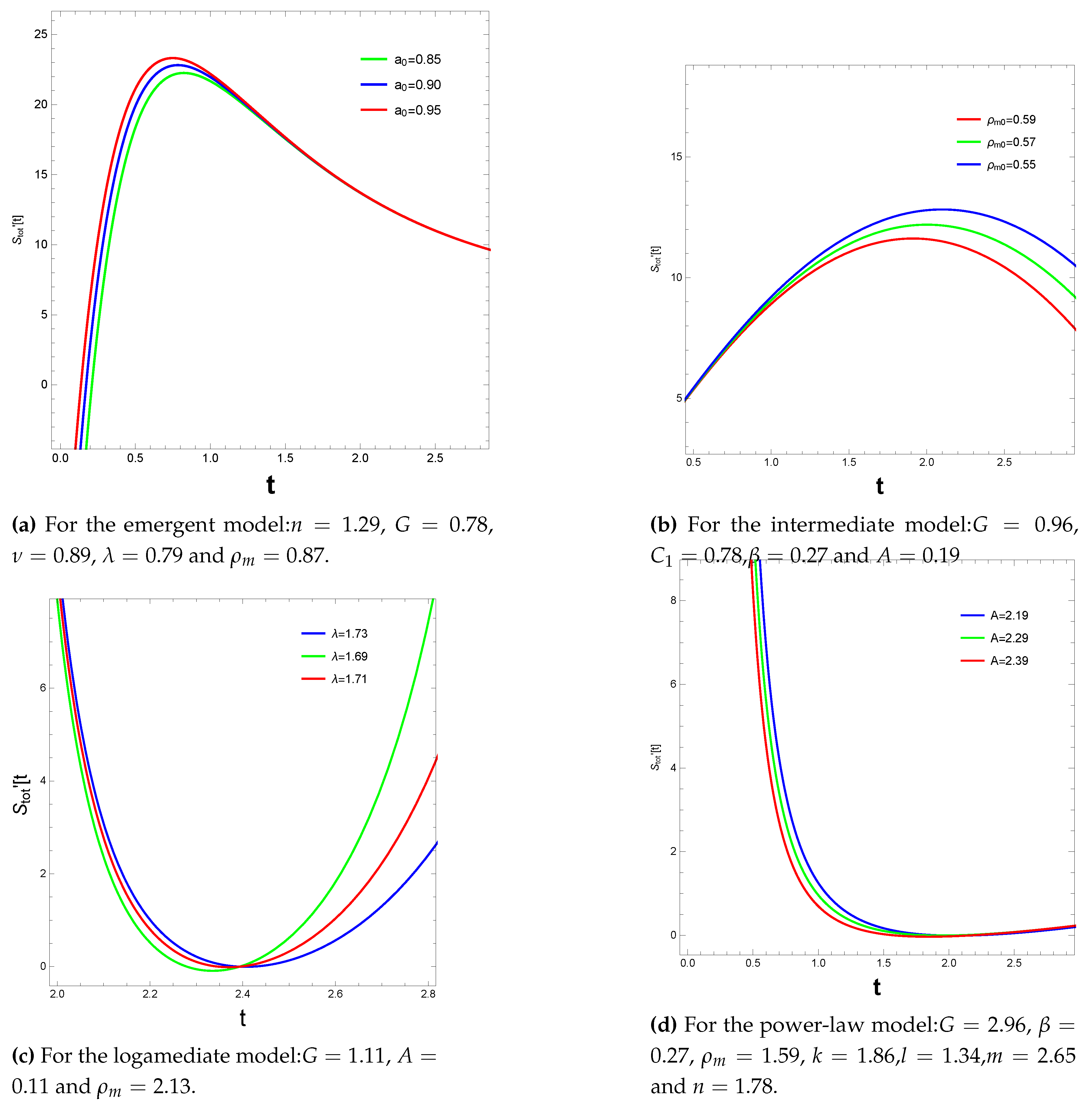
Thus, these are the general equations one may use while investigating the validity of GSL while considering the cosmologies. In our work, we have considered the three different scale factors used previously viz. emergent, intermediate and logamediate that yield different formulations of in terms of t. In addition, various reconstructed forms of density() and pressure() that we have formulated in the previous section corresponding to different scale factors() and the power law model were also substituted in the appropriate equations which helped us obtain three different mathematical forms of , each corresponding to the four different models we have reconstructed in the previous section. The graphs obtained by plotting the total entropy change against time are shown in Figure 9 and Figure 10. In all the plots, we observe that the is staying at a positive level which indicates the validity of GSL for all our cosmological models.
5. Conclusions
The authors [127] showed that the entropic DE and the generalized HDE are equivalent and extended this to the case where the entropy functions’ respective exponents are permitted to change in response to the universe’s expansion. They considered several entropic DE models, including the Tsallis, Rényi, and Sharma-Mittal entropic DEs. The authors [128] established the equivalence between the Barrow entropic dark energy and the generalized HDE extending to the case where the exponent of the Barrow entropy permits to fluctuate with the cosmological expansion of the universe. After extracting the modified Friedmann equations, which contain new terms quantified by the non-extensive exponent and have regular CDM cosmology as a subcase, [129] provided a modified cosmic scenario that results from applying non-extensive thermodynamics with variable exponent.
This paper presents an analysis of gravity theory for a homogeneous and isotropic metric. We have focused mainly on the investigation into the reconstruction of four different models using different forms of scale factor and a model based on the power-law-like form of f. The three scale factors chosen are emergent, intermediate, and logamediate and the background fluid for reconstruction is considered to be the Holographic Ricci Dark Energy(HRDE), a particular case of a highly generalized holographic dark energy, namely Nojiri-Odintsov HDE [130]. In the first phase of our study, we examined four cosmological scenarios where we obtained the reconstructed densities and pressure, the EoS parameters, and the squared speed of sound for the different models. Utilising Friedmann’s equations and the HRDE we have reconstructed the function f for the three different choices of the scale factor. The following were the main results:
- In the case of the emergent scale factor, we see(cf. Figure 1) that the function is a decreasing function which is asymptotically tending towards 1 with the increase in t. The EoS parameter (see Figure 2) shows a phantom behaviour and tends to with the increase in time t. The squared speed of sound shows a decrease in value with time but stays positive which indicates the stability of the density perturbations and possibly, the model.
- For the second model with the intermediate scale factor we observe that the function f increases with time(cf. Figure 4). From Figure 5, we see that the EoS parameter shows a quintessence behaviour at a later stage and shows acceleration() in the early stage. The squared speed of sound is greater than 0 when plotted against time(cf. Figure 6).
- In our third model, we have chosen the logamediate scale factor and proceeded with the reconstruction of gravity like the previous two models. The reconstructed function when plotted against time (cf. Figure 7) shows a monotonic decrease with time and asymptotically tends to 0 at . A transition from quintessence to phantom behaviour is exhibited by the EoS parameter in this case(see Figure 8)
- For our fourth cosmological model, we have taken a power-law-like function for the torsion and boundary scalar. Choosing the intermediate scale factor, we have reconstructed the EoS parameter, the methodology for which have been discussed in subSection 3.4. We have obtained the EoS parameters for 3 different cases based on the constants in the functional form of that we assumed. The figures (cf. Figure 9) show that for different cases, the behavior of the EoS parameter is mainly phantom-like, a result that is similar to the findings by [131].
In the last part of our study, we have focused on the thermodynamical analysis of all four models presented in the previous section. This has been done by considering the apparent horizon and using the different reconstructed densities and pressures from each of the four models to validate the Generalised Second Law of Thermodynamics(GSLT) with and without using the first law. Figure 10 and Figure 11 show the plot of against time and it can be seen that for all the models the GSLT is satisfied. We wish to expand our study to include the event horizon and investigate our model’s thermodynamical consistency by examining the GSLT’s validity as part of our future work. In this context, we need to mention an important study by [132] in which the authors have examined the validity of GSLT in the context of scalar-tensor gravity theory at the event horizon with modified Hawking temperature. Additionally, we also draw attention to another important work done by [133] wherein they have reviewed finite-time cosmological singularities in various cosmological contexts and have shown the nature of these singularities. In future works, we wish to explore the possibilities of our model giving rise to such singularities.
Author Contributions
The formal analysis and the first draft has been prepared by the first author. Conceptualisation, formal analyis and supervision was done by Surajit Chattopadhyay.
Acknowledgments
The first author sincerely acknowledges the financial support from GLA University, Mathura for participation in ICGAC 2024. Most of the study was completed at the Inter-University Centre for Astronomy and Astrophysics (IUCAA), Pune, India, where the authors were hosted during their December 2023-January 2024 trip. The authors are grateful for the hospitality.
Conflicts of Interest
The authors hereby declare that there is no conflict of interest associated with this work.
References
- Sami, M. and Myrzakulov, R. Late-time cosmic acceleration: ABCD of dark energy and modified theories of gravity. Int. J. Mod. Phys. D 2016, 25, 163001. [Google Scholar] [CrossRef]
- Adil, S.A.; Gangopadhyay, M.R.; Sami, M. and Sharma, M. K. Late-time acceleration due to a generic modification of gravity and the Hubble tension Phys. Rev. D 2021, 10, 163001. [Google Scholar]
- Park, M.; Zurek, K.M. and Watson, S. Unified approach to cosmic acceleration Phys. Rev. D 2010, 81, 124008. [Google Scholar]
- Nojiri, S.I. and Odintsov, S.D. Unifying phantom inflation with late-time acceleration: Scalar phantom–non-phantom transition model and generalized holographic dark energy. Phys. Rev. D 2006, 38, 1285–1304. [Google Scholar]
- Riess, A.G.; Filippenko, A.V.; Challis, P.; Clocchiatti, A.; Diercks, A.; Garnavich, P.M.; Gilliland, R.L.; Hogan, C.J.; Jha, S.; Kirshner, R.P. and Leibundgut, B.R.U.N.O. Observational evidence from supernovae for an accelerating universe and a cosmological constant. AJ 1998, 116, 1009. [Google Scholar] [CrossRef]
- Permutter, S.; Aldering, G.; Goldhaber, G.; Knop, R.A.; Nugent, P. and Castro, P.G. Measurements of omega and lambda from 42 high redshift supernovae. ApJ 1999, 517, 565. [Google Scholar] [CrossRef]
- Weinberg, D.H.; Mortonson, M.J.; Eisenstein, D.J.; Hirata, C.; Riess, A.G. and Rozo, E. Observational probes of cosmic acceleration. Phys. Rep. 2013, 530, 87–255. [Google Scholar] [CrossRef]
- Haridasu, B.S.; Luković, V.V.; D’Agostino, R. and Vittorio, N. Strong evidence for an accelerating universe. Phys. Rep. 2017, 600, L1. [Google Scholar]
- Copeland, E.J.; Sami, M.; and Tsujikawa, S. Dynamics of dark energy. Int. J. Mod. Phys. D 2006, 15, 1753–1935. [Google Scholar] [CrossRef]
- Li, M.; Li, X.D.; Wang, S and Wang, Y. Dark Energy. Commun. Theor. Phys. 2011, 563, 525. [Google Scholar] [CrossRef]
- Dark Energy Survey Collaboration:, Abbott, T. ; Abdalla, F.B.; Aleksić, J.; Allam, S.; Amara, A.; Bacon, D.; Balbinot, E.; Banerji, M.; Bechtol, K.; and Benoit-Lévy, A. The Dark Energy Survey: more than dark energy–an overview. Mon. Not. R. Astron. Soc. 2016, 460, 270–1299. [Google Scholar]
- Amendola, L. and Tsujikawa, S. Dark energy: theory and observations; Cambridge University Press: Cambridge, United Kingdom, 2010. [Google Scholar]
- Frieman, J.A.; Turner, M.S. and Huterer, D. Strong evidence for an accelerating universe. Annu. Rev. Astron. Astrophys. 2008, 46, 385–432. [Google Scholar] [CrossRef]
- Huterer, D. and Turner, M.S. Probing dark energy: Methods and strategies. Phys. Rev. D 2001, 64, 123527. [Google Scholar] [CrossRef]
- Carroll, S.M. The cosmological constant. Living Rev. Relativ. 2001, 4, 1–56. [Google Scholar] [CrossRef]
- Peebles, P.J.E. and Ratra, B. The cosmological constant and dark energy Rev. Mod. Phys. 2003, 75, 559. [Google Scholar]
- Calderon, R.; Shafieloo, A.; Hazra, D.K. and Sohn, W. On the consistency of Λ CDM with CMB measurements in light of the latest Planck, ACT and SPT data. J. Cosmol. Astropart. Phys. 2023, 2023, 059. [Google Scholar] [CrossRef]
- Xu, T.; Chen, Y.; Xu, L. and Cao, S. Comparing the scalar-field dark energy models with recent observations. Phys. Dark Universe 2022, 36, 101023. [Google Scholar] [CrossRef]
- Calcagni, G. and Liddle, A.R. Tachyon dark energy models: Dynamics and constraints. Phys. Rev. D. 2006, 74, 043528. [Google Scholar] [CrossRef]
- Sultana, S.; Güdekli, E. and Chattopadhyay, S. Some versions of Chaplygin gas model in modified gravity framework and validity of generalized second law of thermodynamics. Z NATURFORSCH A 2024, 79, 51–70. [Google Scholar] [CrossRef]
- Chattopadhyay, S. A study on the bouncing behavior of modified Chaplygin gas in presence of bulk viscosity and its consequences in the modified gravity framework. Int. J. Geom. Methods Mod. Phys. 2017, 14, 1750181. [Google Scholar] [CrossRef]
- Chokyi, K.K. and Chattopadhyay, S. A truncated scale factor to realize cosmological bounce under the purview of modified gravity. Astron. Nachr. 2023, 344, e220119. [Google Scholar] [CrossRef]
- Saha, S. and Chattopadhyay, S. Realization of bounce in a modified gravity framework and information theoretic approach to the bouncing point. Universe 2023, 9, 136. [Google Scholar] [CrossRef]
- Pasqua, A.; Chattopadhyay, S. and Myrzakulov, R. Consequences of three modified forms of holographic dark energy models in bulk–brane interaction Can. J. Phys. 2018, 96, 112-125.
- Brax, P.; van de Bruck, C. and Davis, A.C. Brane world cosmology. Rep. Prog. Phys. 2004, 67, 2183. [Google Scholar] [CrossRef]
- Guenther, U. and Zhuk, A. Phenomenology of brane-world cosmological models. Rep. Prog. Phys. 2004. [Google Scholar]
- Ishak, M. Testing general relativity in cosmology. Living Rev. Relativ. 2019, 22, 1–204. [Google Scholar] [PubMed]
- Shankaranarayanan, S. and Johnson, J.P. Modified theories of gravity: Why, how and what? Gen. Relativ. Gravit. 2022, 54, 44. [Google Scholar] [CrossRef]
- Lobo, F.S. The dark side of gravity: Modified theories of gravity. arXiv arXiv:0807.1640.
- Paul, B.C.; Debnath, P.S. and Ghose, S. Accelerating universe in modified theories of gravity. Phys. Rev. D 2009, 79, 083534. [Google Scholar] [CrossRef]
- Sbisà, F. Modified Theories of Gravity. arXiv preprint arXiv:1406.3384. 2014, arXiv:1406.3384. [Google Scholar]
- Capozziello, S. and De Laurentis, M. Extended theories of gravity. Phys. Rep. 2011, 509, 167–321. [Google Scholar] [CrossRef]
- Capozziello, S.; Lobo, F.S. and Mimoso, J.P. Generalized energy conditions in extended theories of gravity. Phys. Rev. D 2015, 91, 124019. [Google Scholar] [CrossRef]
- Capozziello, S. and Francaviglia, M. Extended theories of gravity and their cosmological and astrophysical applications. Phys. Rev. D 2008, 40, 357–420. [Google Scholar]
- Nojiri, S.I. and Odintsov, S. D. Introduction to modified gravity and gravitational alternative for dark energy Int. J. Geom. Methods Mod. Phys. 2007, 4, 115–145. [Google Scholar]
- Wands, D. Extended gravity theories and the Einstein–Hilbert action Class. Quantum Gravity 1994, 11, 269. [Google Scholar] [CrossRef]
- Capozziello, S.; Cardone, V.F. and Salzano, V. Cosmography of f (R) gravity. Phys. Rev. D 2008, 78, 063504. [Google Scholar] [CrossRef]
- Sotiriou, T.P. and Faraoni, V. Modified Theories of Gravity. Rev. Mod. Phys. 2010, 82, 451–497. [Google Scholar] [CrossRef]
- Karmakar, S.; Chattopadhyay, S. and Radinschi, I. A holographic reconstruction scheme for f (R) gravity and the study of stability and thermodynamic consequences. New Astron. 2020, 76, 101321. [Google Scholar] [CrossRef]
- Hwang, J.C. and Noh, H. f(R) gravity theory and CMBR constraints. Phys. Lett. B 2001, 506, 13–19. [Google Scholar]
- Bamba, K.; Nojiri, S.I. , Odintsov, S.D. and Saez-Gomez, D. Inflationary universe from perfect fluid and F(R) gravity and its comparison with observational data. Phys. Rev. D 2014, 90, 124061. [Google Scholar] [CrossRef]
- Vainio, J. and Vilja, I. f (R) gravity constraints from gravitational waves. Gen. Relativ. Gravit. 2017, 49, 1–10. [Google Scholar] [CrossRef]
- Capozziello, S.; Piedipalumbo, E.; Rubano, C. and Scudellaro, P. Testing an exact f (R)-gravity model at Galactic and local scales. Astron. Astrophys. 2009, 505, 21–28. [Google Scholar] [CrossRef]
- Ky, N.A.; Van Ky, P.; and Van, N.T.H. Testing the f(R)-theory of gravity. arXiv preprint arXiv:1904.04013. 2019, arXiv:1904.04013. [Google Scholar] [CrossRef]
- Nojiri, S.; Odintsov, S.D. and Oikonomou, V. Modified gravity theories on a nutshell: Inflation, bounce and late-time evolution. Phys. Rep. 2017, 692, 1–104. [Google Scholar] [CrossRef]
- Chattopadhyay, S. A study on the interacting Ricci dark energy in f (R, T) gravity. Proc. Natl. Acad. Sci. India - Phys. Sci. 2014, 84, 87–93. [Google Scholar] [CrossRef]
- Pasqua, A.; Chattopadhyay, S. and Myrzakulov, R. arXiv preprint arXiv:1306.0991. 2013, arXiv:1306.0991. [Google Scholar]
- Sharif, M. and Zubair, M. Study of thermodynamic laws in f (R, T, RμνTμν) gravity. J. Cosmol. Astropart. Phys. 2013, 2013, 42. [Google Scholar] [CrossRef]
- Gao, X. Unifying framework for scalar-tensor theories of gravity. Phys. Rev. D 2014, 90, 081501. [Google Scholar] [CrossRef]
- Fujii, Y. and Maeda, K.I. The scalar-tensor theory of gravitation.; Cambridge University Press: Cambridge, United Kingdom, 2003. [Google Scholar]
- Wagoner, R.V. Scalar-tensor theory and gravitational waves. Phys. Rev. D 1970, 1, 3209. [Google Scholar] [CrossRef]
- Nojiri, S.I. and Odintsov, S.D. Unified cosmic history in modified gravity: from F (R) theory to Lorentz non-invariant models. Phys. Rep. 2011, 505, 59–144. [Google Scholar] [CrossRef]
- De Andrade, V.C.; Guillen, L.C.T. and Pereira, J.G. Teleparallel gravity: an overview. In he Ninth Marcel Grossmann Meeting: On Recent Developments in Theoretical and Experimental General Relativity, Gravitation and Relativistic Field Theories, 2002; pp. 1022-1023.
- Bahamonde, S. , Böhmer, C.G. and Krššák, M. New classes of modified teleparallel gravity models. Phys. Lett. B 2017, 775, 37–43. [Google Scholar] [CrossRef]
- Garecki, J. Teleparallel equivalent of general relativity: a critical review. arXiv preprint arXiv:1010.2654. 2010, arXiv:1010.2654. [Google Scholar]
- Zhang, J. and Khan, G. From Hessian to Weitzenböck: Manifolds with torsion-carrying connections. Inf. Geom. 2019, 2, 77–98. [Google Scholar] [CrossRef]
- Ong, Y.C.; Izumi, K.; Nester, J.M. and Chen, P. Problems with propagation and time evolution in f (T) gravity. Phys. Rev. D 2013, 88, 024019. [Google Scholar] [CrossRef]
- Li, B.; Sotiriou, T.P. and Barrow, J.D. f (T) gravity and local Lorentz invariance. Phys. Rev. D 2011, 83, 064035. [Google Scholar] [CrossRef]
- Yang, R.J. New types of f (T) gravity EUR. PHYS. J. C 2011, 71, 59–144. [Google Scholar]
- Liu, D. and Reboucas, M.J. New types of f (T) gravity Phys. Rev. 2012, 86, 083515. [Google Scholar]
- Yang, R.J. New types of f (T) gravity EUR. PHYS. J. C 2011, 71, 59–144. [Google Scholar]
- Li, M.; Miao, R.X. and Miao, Y.G. Degrees of freedom of f (T) gravity. J. High Energy Phys 2011, 2011, 1–15. [Google Scholar] [CrossRef]
- Krššák, M. and Saridakis, E.N. The covariant formulation of f (T) gravity Class. QuantumGravity. 2016, 33, 11509. [Google Scholar]
- Bahamonde, S.; Böhmer, C.G. and Krššák, M. New classes of modified teleparallel gravity models Phys. Lett. B 2017, 775, 37–43. [Google Scholar]
- Tamanini, N. and Boehmer, C.G. Good and bad tetrads in f (T) gravity. Phys. Rev. D 2012, 86, 044009. [Google Scholar] [CrossRef]
- Bahamonde, S.; Böhmer, C.G. and Wright, M. Modified teleparallel theories of gravity. Phys. Rev. D 2015, 92, 104042. [Google Scholar] [CrossRef]
- Salako, I.G.; Rodrigues, M.E.; Kpadonou, A.V.; Houndjo, M.J.S. and Tossa, J. ΛCDM model in f (T) gravity: reconstruction, thermodynamics and stability. J. Cosmol. Astropart. Phys. 2013, 2013, 60. [Google Scholar]
- Setare, M.R. and Mohammadipour, N. Can f (T) gravity theories mimic ΛCDM cosmic history. J. Cosmol. Astropart. Phys. 2013, 1, 15. [Google Scholar]
- Susskind, L. The world as a hologram. J. Math. Phys. 1995, 36, 6377–6396. [Google Scholar] [CrossRef]
- Stephens, C.R.; Hooft, G.T. and Whiting, B.F. Black hole evaporation without information loss. Class. Quantum Gravity 1994, 11, 621. [Google Scholar] [CrossRef]
- Witten, E. Anti de Sitter space and holography. arXiv preprint hep-th/9802150. 2015. [Google Scholar]
- Susskind, L. and Witten, E. The holographic bound in anti-de Sitter space. arXiv preprint hep-th/9805114. 1998. [Google Scholar]
- Fischler, W. and Susskind, L. Holography and cosmology. arXiv preprint hep-th/9806039. 1998. [Google Scholar]
- Nojiri, S.I.; Odintsov, S.D. and Paul, T. Different faces of generalized holographic dark energy. Symmetry 2021, 13, 928. [Google Scholar] [CrossRef]
- Sheykhi, A. Holographic scalar field models of dark energy. Phys. Rev. D 2011, 84, 107302. [Google Scholar] [CrossRef]
- Cruz, M. and Lepe, S. Modeling holographic dark energy with particle and future horizons. Nucl. Phys. B 2020, 956, 115017. [Google Scholar] [CrossRef]
- Sadri, E. and Khurshudyan, M. An interacting new holographic dark energy model: Observational constraints. Int. J. Mod. Phys. D 2019, 28, 1950152. [Google Scholar] [CrossRef]
- Moradpour, H.; Ziaie, A.H. and Zangeneh, M.K. Generalized entropies and corresponding holographic dark energy models. EUR. PHYS. J. C 2020, 80, 732. [Google Scholar] [CrossRef]
- Myung, Y.S. and Seo, M.G. Origin of holographic dark energy models. Phys. Lett. B 2009, 671, 435–439. [Google Scholar] [CrossRef]
- Li, M.; Li, X.D.; Wang, S. and Zhang, X. Holographic dark energy models: A comparison from the latest observational data. Nucl. Phys. B 2009, 2009, 036. [Google Scholar]
- Nojiri, S.I.; Odintsov, S.D.; Oikonomou, V.K. and Paul, T. Unifying holographic inflation with holographic dark energy: A covariant approach. Phys. Rev. D 2009, 102, p.023540.
- Nojiri, S.I.; Odintsov, S.D. and Paul, T. Holographic realization of constant roll inflation and dark energy: An unified scenario. Phys. Lett. B 2023, 841, 137926. [Google Scholar] [CrossRef]
- Gao, C.; Wu, F.; Chen, X. and Shen, Y.G. Holographic dark energy model from Ricci scalar curvature. Phys. Rev. D 2009, 79, 043511. [Google Scholar] [CrossRef]
- Nojiri, S.I. and Odintsov, S.D. Covariant generalized holographic dark energy and accelerating universe. EUR. PHYS. J. C 2017, 77, 1–8. [Google Scholar] [CrossRef]
- Nojiri, S.I. and Odintsov, S.D. Unifying phantom inflation with late-time acceleration: Scalar phantom–non-phantom transition model and generalized holographic dark energy. Gen. Relativ. Gravit. 2006, 38, 1285–1304. [Google Scholar] [CrossRef]
- Feng, C.J. Ricci dark energy in Brans-Dicke theory. arXiv preprint arXiv:0806.0673. 2008, arXiv:0806.0673. [Google Scholar]
- Odintsov, S.D.; Paul, T. and SenGupta, S. Second law of horizon thermodynamics during cosmic evolution. Phys. Rev. D 2024, 104, 103515. [Google Scholar] [CrossRef]
- Cai, R.G. and Kim, S.P. First law of thermodynamics and Friedmann equations of Friedmann-Robertson-Walker universe. Phys. Rev. D 2005, 2005, 050. [Google Scholar]
- Akbar, M. and Cai, R.G. Thermodynamic behavior of the Friedmann equation at the apparent horizon of the FRW universe. Phys. Rev. D 2007, 75, 084003. [Google Scholar] [CrossRef]
- Sheykhi, A.; Wang, B. and Cai, R.G. Deep connection between thermodynamics and gravity in Gauss-Bonnet braneworlds. Phys. Rev. D 2007, 76, 023515. [Google Scholar] [CrossRef]
- Sheykhi, A.; Wang, B. and Cai, R.G. Thermodynamical properties of apparent horizon in warped DGP braneworld. Nucl. Phys. B 2007, 779, 1–12. [Google Scholar] [CrossRef]
- Cai, R.G. and Cao, L.M. Unified first law and the thermodynamics of the apparent horizon in the FRW universe. Phys. Rev. D 2007, 75, 064008. [Google Scholar] [CrossRef]
- Akbar, M. and Cai, R.G. Thermodynamic behavior of field equations for f (R) gravity. Phys. Lett. B 2007, 648, 243–248. [Google Scholar] [CrossRef]
- Cai, R.G.; Cao, L.M.; Hu, Y.P. and Kim, S.P. Generalized Vaidya spacetime in Lovelock gravity and thermodynamics on the apparent horizon. Phys. Rev. D 2008, 78, 124012. [Google Scholar] [CrossRef]
- Nojiri, S.I.; Odintsov, S.D.; Paul, T. and SenGupta, S. Horizon entropy consistent with the FLRW equations for general modified theories of gravity and for all equations of state of the matter field Phys. Rev. D 2024, 109, 043532. [Google Scholar]
- Miao, R.X.; Li, M. and Miao, Y.G. Violation of the first law of black hole thermodynamics in f (T) gravity. J. Cosmol. Astropart. Phys. 2011, 2011, 033. [Google Scholar] [CrossRef]
- Bamba, K.; Jamil, M.; Momeni, D. and Myrzakulov, R. Generalized second law of thermodynamics in f (T) gravity with entropy corrections. Astrophys. Space Sci. 2013, 344, 259–267. [Google Scholar] [CrossRef]
- Karami, K. and Abdolmaleki, A. Generalized second law of thermodynamics in f (T) gravity. J. Cosmol. Astropart. Phys. 2012, 2012, 007. [Google Scholar] [CrossRef]
- Farrugia, G. and Said, J.L. Stability of the flat FLRW metric in f (T) gravity. Phys. Rev. D 2016, 94, 124054. [Google Scholar] [CrossRef]
- Caruana, M.; Farrugia, G. and Levi Said, J. Cosmological bouncing solutions in f (T, B) gravity. EUR. PHYS. J. C 2020, 80, 640. [Google Scholar] [CrossRef]
- Bahamonde, S. and Capozziello, S. Noether symmetry approach in f (T, B) teleparallel cosmology EUR. PHYS. J. C 2017, 77,1-10.
- Franco, G.A.R.; Escamilla-Rivera, C. and Levi Said, J. Stability analysis for cosmological models in f (T, B) gravity. EUR. PHYS. J. C 2020, 80, 677. [Google Scholar] [CrossRef]
- Escamilla-Rivera, C. and Said, J.L. Cosmological viable models in f (T, B) theory as solutions to the H0 tension. Class. Quantum Gravity 2020, 37, 165002. [Google Scholar] [CrossRef]
- Chattopadhyay, S. and Pasqua, A. Various aspects of interacting modified holographic Ricci dark energy. Indian J. Phys. 2013, 87, 1053–1057. [Google Scholar] [CrossRef]
- Ellis, G.F. and Maartens, R. The emergent universe: Inflationary cosmology with no singularity. Class. Quantum Gravity 2003, 21, 223. [Google Scholar]
- Ellis, G.F.; Murugan, J. and Tsagas, C.G. The emergent universe: an explicit construction. Class. Quantum Gravity 2003, 21, 233. [Google Scholar]
- Mulryne, D.J.; Tavakol, R.; Lidsey, J.E. and Ellis, G.F. An emergent universe from a loop. Phys. Rev. D 2005, 71, 123512. [Google Scholar] [CrossRef]
- Carter, B.M. and Neupane, I.P. Thermodynamics and stability of higher dimensional rotating (Kerr-) AdS black holes. Phys. Rev. D 2005, 72, 1043534. [Google Scholar] [CrossRef]
- Mukherjee, S.; Paul, B.C.; Dadhich, N.K.; Maharaj, S.D. and Beesham, A. Emergent universe with exotic matter. Class. Quantum Gravity 2006, 23, 6927. [Google Scholar] [CrossRef]
- Chattopadhyay, S. and Debnath, U. Role of generalized Ricci dark energy on a Chameleon field in the emergent universe. Can. J. Phys. 2011, 89, 941–948. [Google Scholar] [CrossRef]
- Hannestad, S. Constraints on the sound speed of dark energy. Phys. Rev. D 2005, 71, 103519. [Google Scholar] [CrossRef]
- Eisenstein, D.J. Dark energy and cosmic sound. New Astron. Rev. 2005, 49, 360–365. [Google Scholar] [CrossRef]
- Barrow, J.D. Graduated inflationary universes. Phys. Lett. B 1990, 235, 40–43. [Google Scholar] [CrossRef]
- Mohajan, H. A brief analysis of de Sitter universe in relativistic cosmology. J. Achiev. Mater. Manuf. Eng. 2017, 2, 1–17. [Google Scholar]
- Tutusaus, I.; Lamine, B.; Blanchard, A.; Dupays, A.; Zolnierowski, Y.; Cohen-Tanugi, J.; Ealet, A.; Escoffier, S.; Le Fèvre, O.; Ilić, S. and Pisani, A. Power law cosmology model comparison with CMB scale information. Phys. Rev. D 2016, 94, 103511. [Google Scholar] [CrossRef]
- Barrow, J.D. and Saich, P. The behaviour of intermediate inflationary universes. Phys. Lett. B 1990, 249, 406–410. [Google Scholar] [CrossRef]
- Barrow, J.D. and Liddle, A.R. Perturbation spectra from intermediate inflation. Phys. Lett. B 1993, 47, R5219. [Google Scholar]
- Rezazadeh, K.; Abdolmaleki, A. and Karami, K. Logamediate inflation in f (T) teleparallel gravity. Astrophys. J. 2017, 836, 228. [Google Scholar] [CrossRef]
- Barrow, J.D. Varieties of expanding universe. Class. Quantum Gravity 1996, 13, 2965. [Google Scholar] [CrossRef]
- Barrow, J.D. and Parsons, P. Inflationary models with logarithmic potentials. Phys. Rev. D 1995, 52, 5576. [Google Scholar] [CrossRef]
- Barrow, J.D. and Nunes, N.J. Dynamics of “logamediate” inflation. Phys. Rev. D 2007, 76, 043501. [Google Scholar] [CrossRef]
- Bahamonde, S. and Capozziello, S. Noether symmetry approach in f (T, B) teleparallel cosmology. EUR. PHYS. J. C 2017, 77, 1–10. [Google Scholar] [CrossRef]
- Das, A.; Chattopadhyay, S. and Debnath, U.. Validity of the generalized second law of thermodynamics in the logamediate and intermediate scenarios of the Universe. Found. Phys. 2012, 42, 266–283. [Google Scholar] [CrossRef]
- Ghosh, R.; Pasqua, A. and Chattopadhyay, S. Generalized second law of thermodynamics in the emergent universe for some viable models of f (T) gravity. EUR. PHYS. J. C 2013, 128, 1–11. [Google Scholar]
- Chakraborty, G.; Chattopadhyay, S.; Güdekli, E. and Radinschi, I. Thermodynamics of Barrow holographic dark energy with specific cut-off. Symmetry 2021, 13, 562. [Google Scholar] [CrossRef]
- Bahamonde, S.; Zubair, M. and Abbas, G. Thermodynamics and cosmological reconstruction in f (T, B) gravity. Phys. Dark Universe 2018, 19, 78–90. [Google Scholar] [CrossRef]
- Nojiri, S.I.; Odintsov, S.D. and Paul, T. Different faces of generalized holographic dark energy. Symmetry 2021, 13, 928. [Google Scholar] [CrossRef]
- Nojiri, S.I.; Odintsov, S.D. and Paul, T. Barrow entropic dark energy: A member of generalized holographic dark energy family. Phys. Lett. B 2022, 825, 136844. [Google Scholar] [CrossRef]
- Nojiri, S.I.; Odintsov, S.D. and Saridakis, E.N. Modified cosmology from extended entropy with varying exponent. EUR. PHYS. J. C 2019, 79, 242. [Google Scholar] [CrossRef]
- Nojiri, S.I. and Odintsov, S.D. Unifying phantom inflation with late-time acceleration: Scalar phantom–non-phantom transition model and generalized holographic dark energy. Gen. Relativ. Gravit. 2006, 38, 1285–1304. [Google Scholar] [CrossRef]
- Escamilla-Rivera, C. and Said, J.L. Cosmological viable models in f (T, B) theory as solutions to the H0 tension. Class. Quantum Gravity 2020, 37, 165002. [Google Scholar] [CrossRef]
- Chetry, B.; Dutta, J. and Abdolmaleki, A. Thermodynamics of event horizon with modified Hawking temperature in scalar-tensor gravity. Gen. Relativ. Gravit. 2018, 50, 1–33. [Google Scholar] [CrossRef]
- de Haro, J.; Nojiri, S.I.; Odintsov, S.D. , Oikonomou V.K. and Pan, S Finite-time cosmological singularities and the possible fate of the Universe. Phys. Rep. 2023, 1034, 1–114. [Google Scholar] [CrossRef]
Figure 1.
Behaviour of (vertical axis) plotted against time t in the case of emergent cosmology.We have taken ,,,,
Figure 1.
Behaviour of (vertical axis) plotted against time t in the case of emergent cosmology.We have taken ,,,,
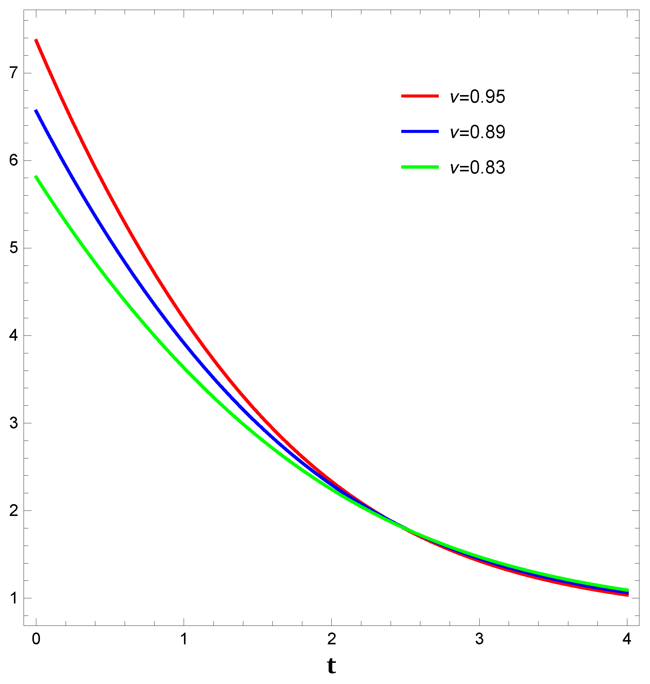
Figure 2.
Behaviour of plotted against time t in the context of the emergent universe. We consider ,,,.
Figure 2.
Behaviour of plotted against time t in the context of the emergent universe. We consider ,,,.
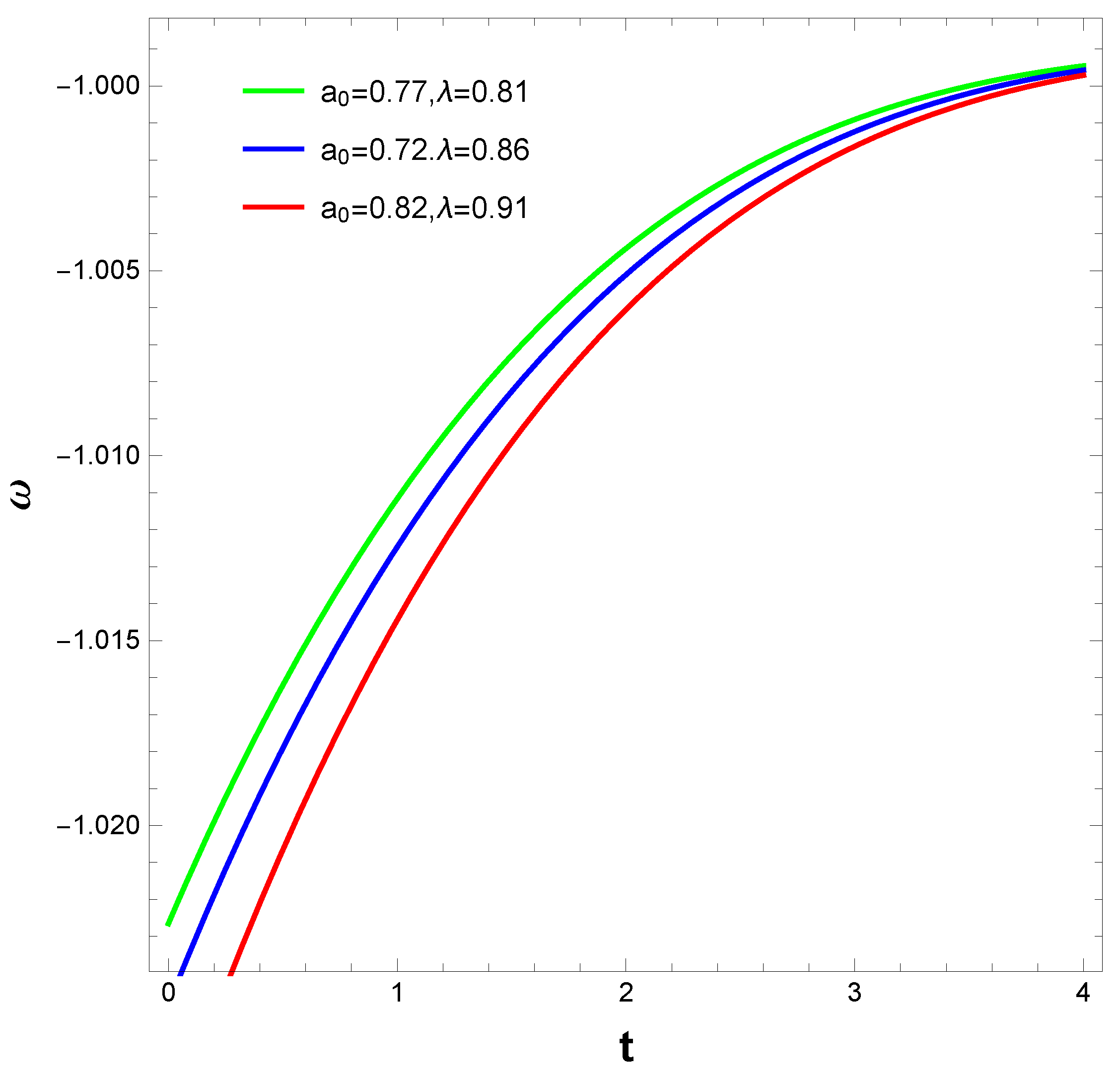
Figure 3.
plotted against time t in the case of emergent scale factor where , , and
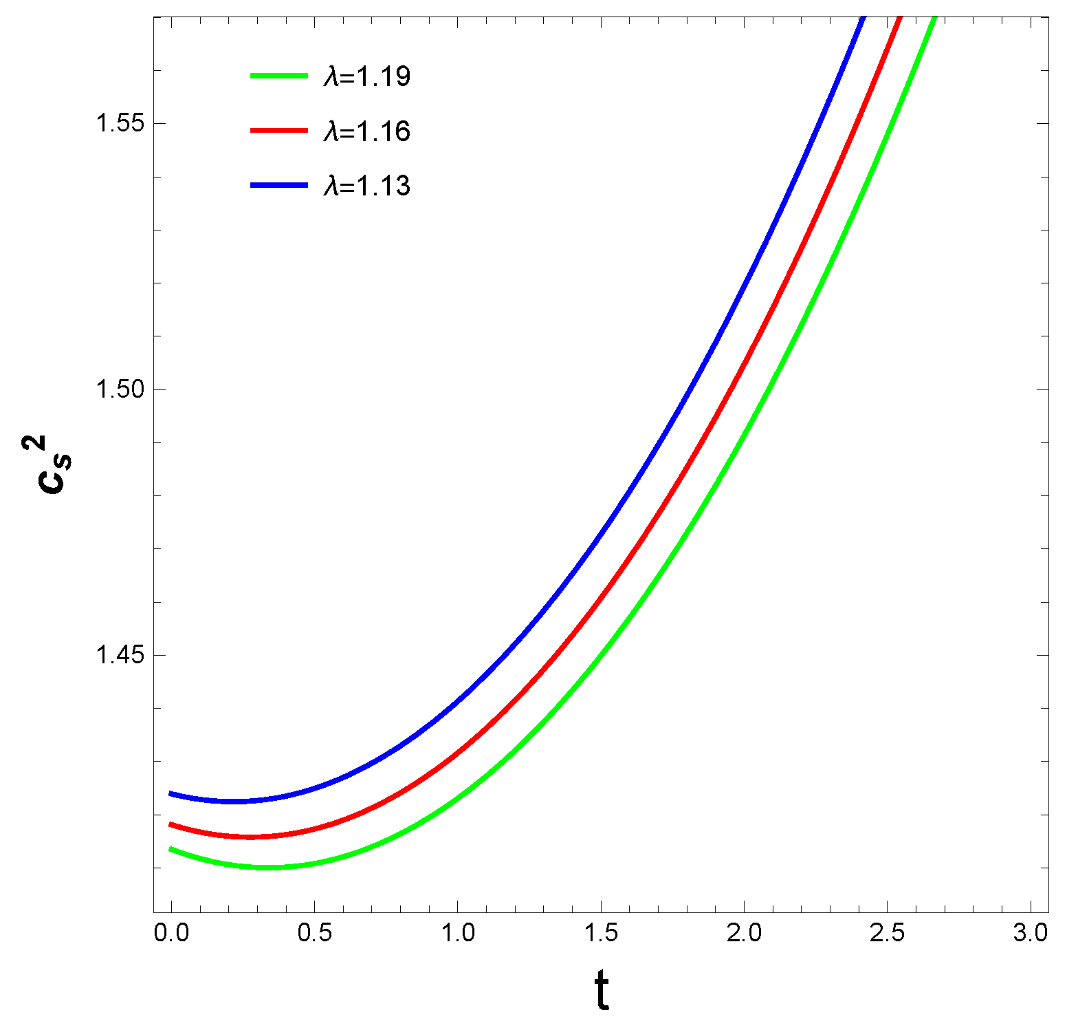
Figure 4.
Behaviour of reconstructed with respect to time t for the intermediate scale factor where , and .
Figure 4.
Behaviour of reconstructed with respect to time t for the intermediate scale factor where , and .
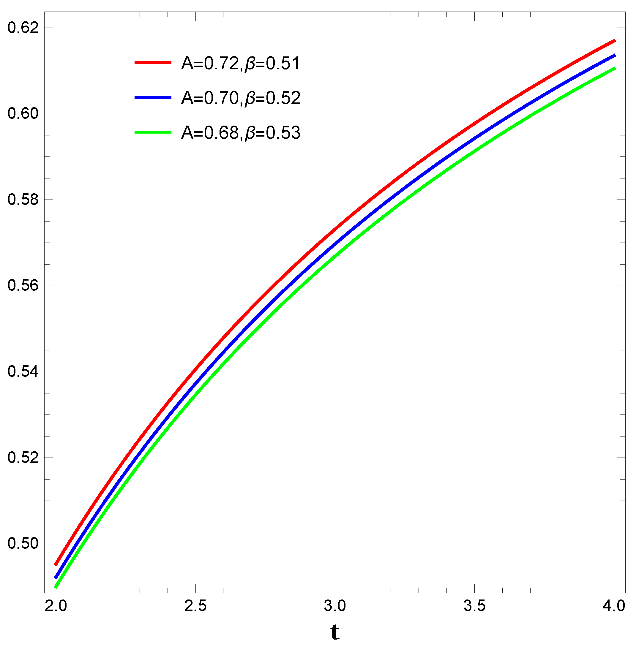
Figure 5.
Behaviour of plotted against time t for the case of intermediate scale factor. Here, ,, and . The purple, orange and green lines correspond to respectively.
Figure 5.
Behaviour of plotted against time t for the case of intermediate scale factor. Here, ,, and . The purple, orange and green lines correspond to respectively.
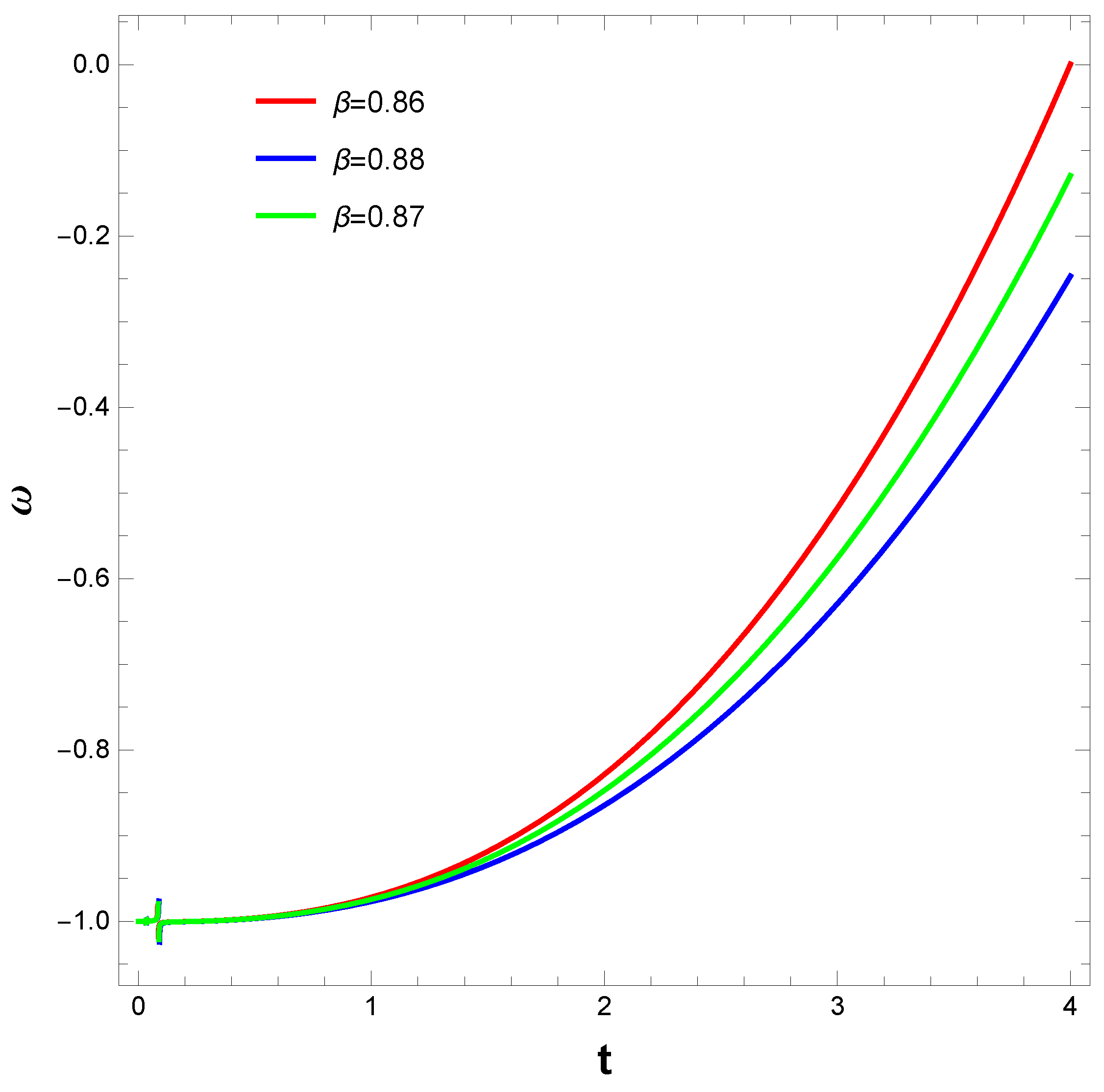
Figure 6.
plotted against time t for the intermediate scale factor. Here, and
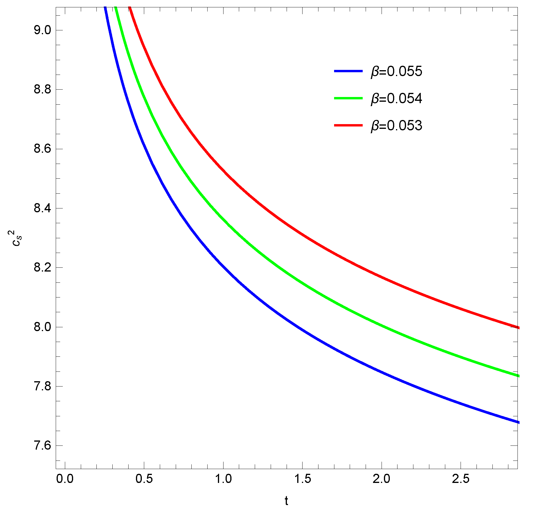
Figure 7.
Behaviour of plotted against time t for the logamediate scale factor. We have taken , and .
Figure 7.
Behaviour of plotted against time t for the logamediate scale factor. We have taken , and .
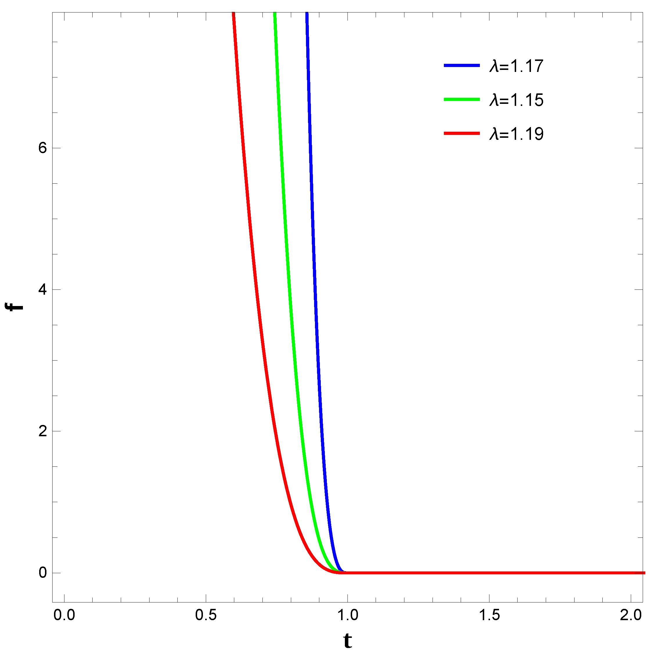
Figure 8.
Behaviour of plotted against time t in case of logamediate model. We have taken , and .
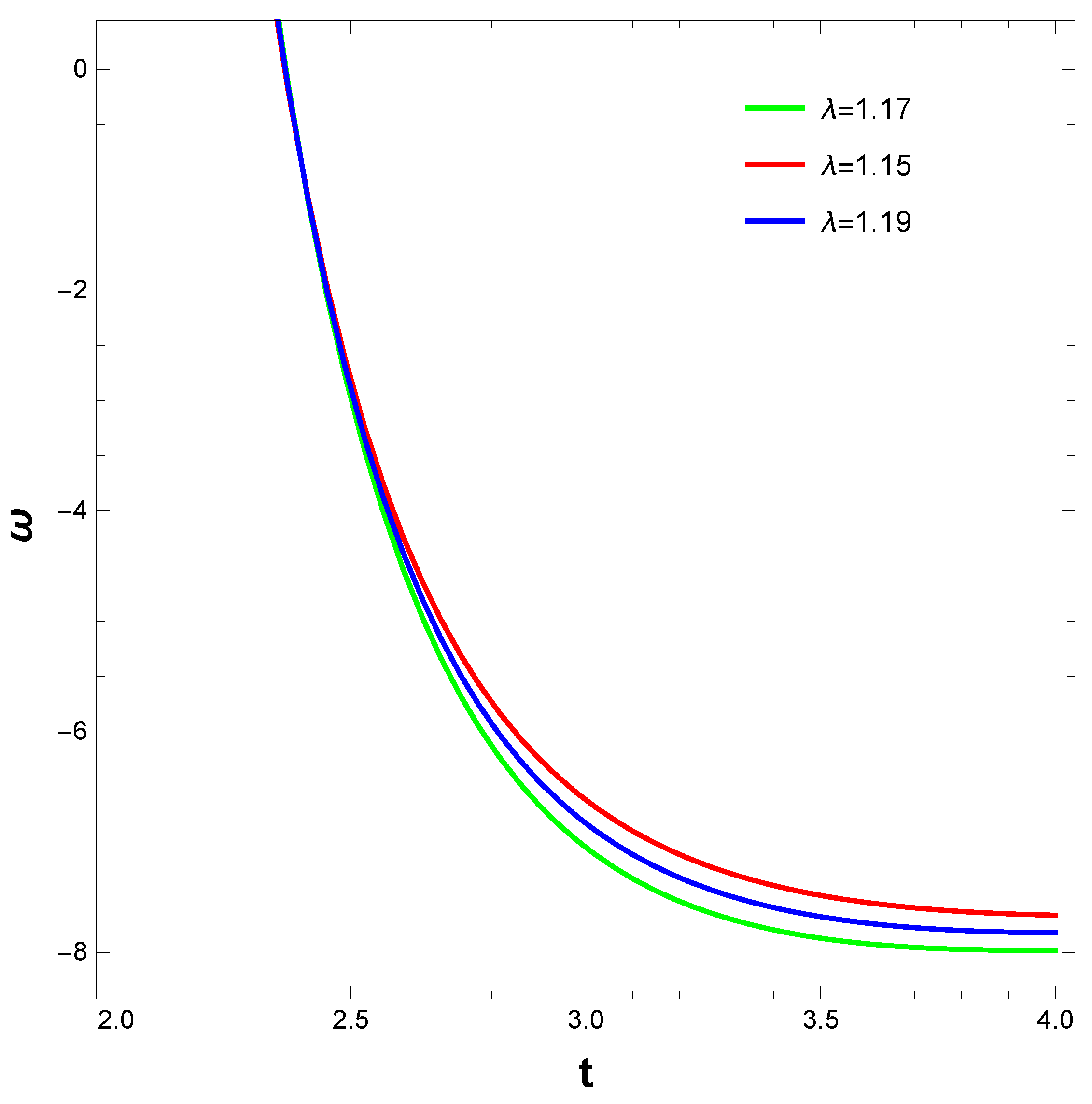
Figure 9.
Evolution of EoS for the power-law model. Left: Case 1: . Middle: Case 2: . Right: Case 3: m(green) and n(blue) take negative values
Figure 9.
Evolution of EoS for the power-law model. Left: Case 1: . Middle: Case 2: . Right: Case 3: m(green) and n(blue) take negative values
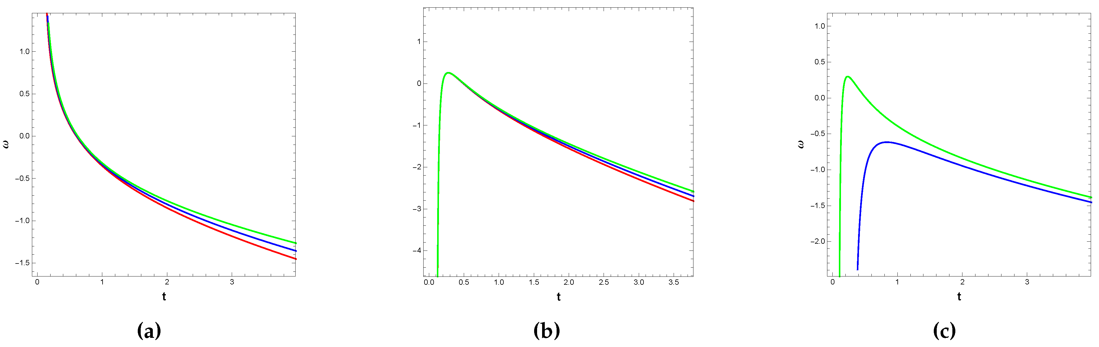
Figure 10.
Time derivative of total entropy plotted against time for the first case, i.e., using the first law.
Figure 10.
Time derivative of total entropy plotted against time for the first case, i.e., using the first law.
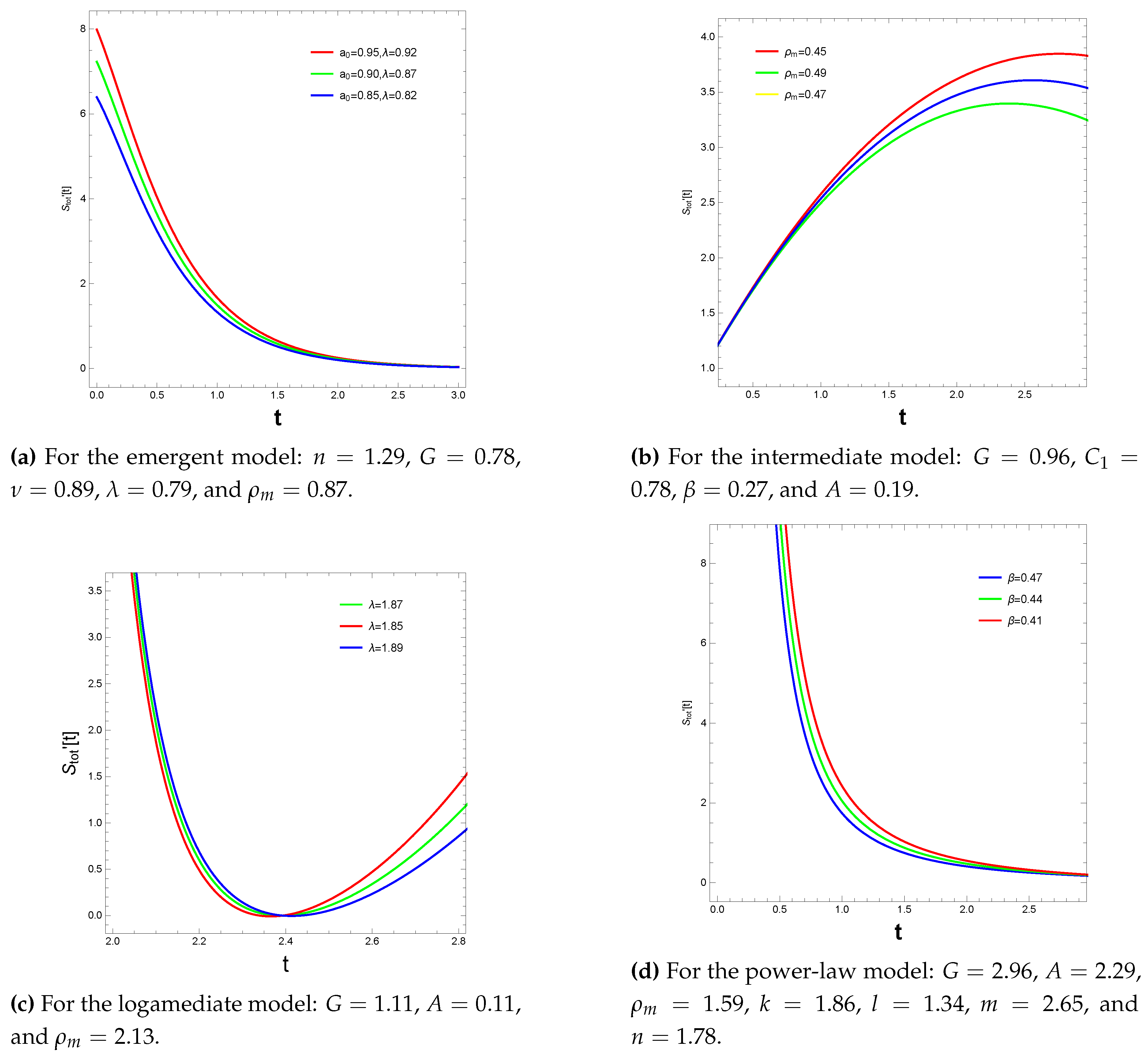
Figure 11.
Time derivative of total entropy plotted against time for the second case i.e without using the first law.
Figure 11.
Time derivative of total entropy plotted against time for the second case i.e without using the first law.
Disclaimer/Publisher’s Note: The statements, opinions and data contained in all publications are solely those of the individual author(s) and contributor(s) and not of MDPI and/or the editor(s). MDPI and/or the editor(s) disclaim responsibility for any injury to people or property resulting from any ideas, methods, instructions or products referred to in the content. |
© 2024 by the authors. Licensee MDPI, Basel, Switzerland. This article is an open access article distributed under the terms and conditions of the Creative Commons Attribution (CC BY) license (http://creativecommons.org/licenses/by/4.0/).
Copyright: This open access article is published under a Creative Commons CC BY 4.0 license, which permit the free download, distribution, and reuse, provided that the author and preprint are cited in any reuse.


