
Submitted:
17 October 2025
Posted:
17 October 2025
You are already at the latest version
Abstract
Accurate land cover mapping is essential for environmental monitoring and agricultural management. Sentinel-2 imagery, with high spatial resolution and open access, provides valuable opportunities for operational classification. Convolutional neural networks (CNNs) have demonstrated state-of-the-art results, yet their adoption is limited by high computational demands and limited methodological transparency.
This study proposes a lightweight CNN for soil–vegetation classification, in Dolj County, Romania. The architecture integrates three convolutional blocks, global average pooling, and dropout, with fewer than 150,000 trainable parameters. A fully documented workflow was implemented, covering preprocessing, patch extraction, training, and evaluation, ad-dressing reproducibility challenges common in deep leaning studies.
Experiments on Sentinel-2 imagery achieved 91.2% overall accuracy and a Cohen’s kappa of 0.82. These results are competitive with larger CNNs while reducing computational requirements by over 90%. Comparative analyses showed improvements over an NDVI baseline and a favorable efficiency–accuracy balance relative to heavier CNNs reported in literature.
These findings highlight the potential of lightweight, transparent deep learning for scala-ble and reproducible land cover monitoring, with prospects for extension to multi-class mapping, multi-temporal analysis, and fusion with complementary data such as SAR. This work provides a methodological basis for operational applications in re-source-constrained environments.
Keywords:
Land Use Land Cover
; Sentinel-2
; Deep Learning
; Remote Sensing
; CNN
; Agricultural Monitoring
; Model Optimization
1. Introduction
Land Use Land Cover (LULC) classification is a key task in remote sensing, providing essential information for environmental monitoring, sustainable agricultural practices, and land management strategies. Reliable and up-to-date land cover maps support decision-making processes at multiple scales, from local agricultural planning to global climate change assessments [11].
Traditional approaches to LULC mapping have relied heavily on vegetation indices such as the Normalized Difference Vegetation Index (NDVI) [24] or on classical machine learning algorithms including Random Forests [1] and Support Vector Machines (SVMs) [5]. While these approaches are computationally efficient and relatively easy to implement, their performance often declines in heterogeneous landscapes, especially in transitional areas where spectral signals from soil and vegetation are mixed [9,10].
With the increasing availability of high-resolution, multi-spectral satellite imagery such as Sentinel-2 [7], more advanced methods have become feasible. Sentinel-2 provides rich spectral information across 13 bands at spatial resolutions ranging from 10 to 60 m, with a revisit time of five days, making it particularly suitable for monitoring agricultural and natural environments. However, leveraging the full potential of such data requires methods capable of capturing both spectral and spatial complexity.
Deep learning, and in particular convolutional neural networks (CNNs), has transformed the analysis of remote sensing imagery [16,26]. CNNs can learn hierarchical representations directly from data [4,13,14], allowing them to integrate spectral and spatial dimensions more effectively than traditional methods. State-of-the-art results have been obtained for tasks including land cover classification, crop monitoring, and vegetation mapping [15,20,22,25,32]. Nevertheless, many CNN-based approaches adopt architectures with millions of parameters, such as ResNet [12] or Xception [4], which impose significant computational demands [13,31].
Recent research has emphasized the development of lightweight CNN architectures that maintain high accuracy while drastically reducing computational complexity [19,20,29]. These architectures are especially relevant for operational applications in resource-constrained settings or for large-scale monitoring efforts where computational efficiency is essential. However, reproducibility continues to be a challenge in the field [23]. Many studies fail to report critical details such as preprocessing steps, training/validation splits, or hyperparameter settings, limiting the extent to which results can be independently verified or transferred to new contexts.
In this paper, we propose a lightweight CNN pipeline for binary classification of soil and vegetation using Sentinel-2 imagery, focusing on Dolj County, Romania. The contributions of this work are threefold:
- Methodological transparency. We provide a fully documented pipeline from data preprocessing to model evaluation, ensuring reproducibility and clarity for future applications.
- Efficiency–accuracy trade-off. We demonstrate that a CNN with fewer than 150,000 parameters can reach competitive accuracy (>91% OA, kappa 0.82), while reducing computational demands by more than 90% compared to conventional CNN architectures.
The focus of this work is not solely on achieving the highest possible accuracy but on demonstrating that lightweight, transparent, and reproducible deep learning pipelines can deliver credible results with operational potential. By addressing the efficiency–reproducibility trade-off, this study aims to contribute to the broader adoption of deep learning methods in remote sensing, particularly for institutions and applications where computational resources are limited.
This study goes beyond introducing yet another lightweight CNN variant by providing a fully transparent and reproducible workflow. Every step, from preprocessing to evaluation, is explicitly documented, ensuring methodological clarity. The proposed model demonstrates a favorable efficiency–accuracy trade-off, achieving competitive accuracy while reducing the number of parameters by over 90%. Thus, the contribution lies not only in model design but also in establishing a baseline framework for operational scalability and reproducibility in remote sensing applications.
2. Related Work
2.1. Traditional Machine Learning Approaches
Classical approaches to land cover classification in remote sensing have long relied on vegetation indices and shallow machine learning algorithms. The Normalized Difference Vegetation Index (NDVI) [24] remains one of the most widely used indicators for vegetation monitoring. While effective in highlighting green biomass, NDVI struggles in transitional zones where soil and vegetation signals overlap.
Machine learning methods such as Random Forests [1] and Support Vector Machines (SVMs) [5] have been extensively applied to land cover mapping. These classifiers are computationally efficient and interpretable, and their use in remote sensing has been widely validated [9]. However, they depend heavily on handcrafted features and spectral indices, limiting their ability to generalize across heterogeneous landscapes [10].
2.2. Deep Learning with CNNs
The adoption of deep learning has significantly advanced remote sensing applications. Convolutional neural networks (CNNs) introduced the capacity to learn hierarchical features directly from raw imagery, enabling joint spectral–spatial representation learning [16,26]. Models such as VGGNet [26], ResNet [12], and Xception [4] have demonstrated strong performance across diverse image classification tasks [13,14,32].
In remote sensing, CNNs have been successfully used for crop classification [25], multi-temporal land cover mapping [15,22], and vegetation monitoring [20]. Nevertheless, their widespread use is constrained by high computational requirements. Standard CNNs often contain millions of trainable parameters, demanding GPUs and large memory, which is impractical for many operational or resource-limited contexts [31].
2.3. Lightweight CNN Architectures
To address these challenges, recent research has explored lightweight CNNs designed to reduce computational complexity without sacrificing performance. Approaches such as MobileNets [13], ShuffleNet [32], and custom lightweight CNNs tailored for remote sensing tasks [19,29] have shown that efficient models can deliver strong results while using only a fraction of the parameters of conventional CNNs.
More recent studies have extended these efforts by developing lightweight Vision Transformers and hybrid CNN–ViT architectures specifically for large-scale remote sensing applications [17].
For example, Wang et al. [29] demonstrated that lightweight CNNs could achieve competitive accuracies in land cover mapping tasks, with parameter reductions exceeding 90%. Similarly, Liu et al. [19] proposed models for resource-constrained applications, showing that lightweight deep learning is feasible for large-scale monitoring.
2.4. Reproducibility and Methodological Transparency
A recurring challenge in remote sensing research is reproducibility. Rocchini et al. [23] highlighted the lack of methodological transparency in many studies, where preprocessing details, training–validation splits, or hyperparameter configurations are omitted. This gap undermines the transferability of models across regions and the comparability of results.
In recent years, there has been increasing emphasis on open data, open-source code, and methodological reporting standards in remote sensing [18,23,33]. For example, multi-sensor fusion studies combining SAR and optical data [30] and recent transformer-based lightweight architectures [2,6] stress the importance of transparent experimental design.
3. Materials and Methods
3.1. Study Area
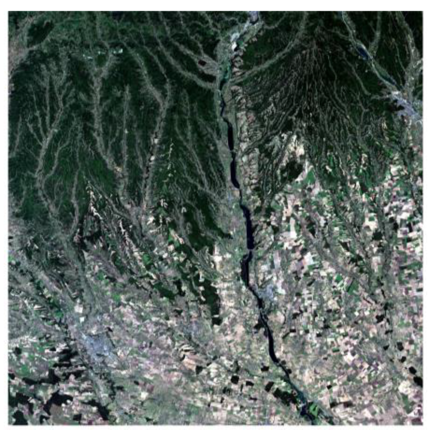
The study was conducted in Dolj County, Romania, an area characterized by a mix of agricultural land, grasslands, and bare soil. The region provides a representative test case for soil–vegetation classification, given its heterogeneous landscape and frequent land use changes.
3.2. Data
Sentinel-2 Level-2A imagery was used, providing 13 spectral bands with spatial resolutions of 10, 20, and 60 m [7]. For this study, we selected the 10 m and 20 m bands most relevant to vegetation and soil discrimination (e.g., B2, B3, B4, B8, B11, B12) (Table 1). The acquisition period covered the 2022 growing season (April–September), ensuring both vegetation and bare soil were captured.
Ground truth data were obtained from field surveys and visual interpretation of high-resolution imagery, annotated into binary classes (soil vs. vegetation).
3.3. Preprocessing
The overall methodological workflow is illustrated in Figure 2, summarizing all steps from raw Sentinel-2 acquisition to final classification.
Preprocessing steps were applied to ensure consistency and suitability of the Sentinel-2 data for CNN-based analysis. The workflow included:
- Atmospheric correction (Sen2Cor).
- Resampling of 20 m bands to 10 m resolution was performed using bilinear interpolation.
- Cloud masking using the Scene Classification Layer (SCL).
- Normalization of reflectance values.
This preprocessing pipeline ensured that the lightweight CNN received harmonized and information-rich inputs while reducing risks of overfitting and bias from spatial dependence.
3.4. CNN Architecture
The proposed lightweight CNN (Figure 5) consisted of three convolutional blocks with ReLU activation and max pooling, followed by a global average pooling layer and a fully connected dense layer with softmax output. Dropout regularization (0.3) was applied to reduce overfitting.
3.5. Training and Evaluation Setup
The dataset was split into training (70%), validation (15%), and test (15%) sets, ensuring spatial independence between sets to avoid overfitting. Training was conducted using the Adam optimizer with an initial learning rate of 0.001 and categorical cross-entropy loss (Table 2). Early stopping based on validation loss was applied to prevent overfitting.
Model performance was assessed using overall accuracy (OA), kappa coefficient, precision, recall, and F1-score. Comparative experiments were conducted against an NDVI threshold baseline and a heavier CNN model.
4. Results
4.1. Classification Accuracy
4.1.1. Overall and Class-Wise Accuracy
The lightweight CNN achieved robust performance on the test dataset. The overall accuracy (OA) was 91.2%, with a Cohen’s kappa coefficient of 0.82, indicating substantial agreement between predictions and reference labels. Macro-averaged precision, recall, and F1-score values exceeded 0.89, confirming the model’s stability across classes (Table 3).
In addition to overall performance, class-wise metrics highlighted slightly better performance for the vegetation class compared to soil (Table 4). This is expected, given the stronger spectral signatures of vegetation in Sentinel-2 bands, particularly in the NIR and red-edge regions.
4.1.2. Error Analysis by NDVI
To further explore misclassification patterns, NDVI values were computed for correctly and incorrectly classified samples (Figure 6). The analysis shows that errors are concentrated in the NDVI range of 0.15–0.25, which corresponds to transitional zones where vegetation is sparse and the spectral signal overlaps with that of bare soil.
NDVI analysis confirms that misclassifications are not random but structurally linked to the intrinsic limitations of optical data in transitional cover conditions.
4.2. Training Dynamics
Training dynamics provide insight into the convergence behavior of the CNN and its ability to generalize.
4.2.1. Accuracy Curves
Training and validation accuracy curves demonstrate stable convergence. The model quickly reached over 85% accuracy within the first 10 epochs and stabilized near 91% by epoch 25. The validation curve closely followed the training curve, indicating minimal overfitting and effective generalization (Figure 7).
4.2.2. Loss Curves
The cross-entropy loss decreased consistently during training, with validation loss stabilizing after epoch 20. Early stopping prevented divergence and ensured that the model did not overfit the training data (Figure 8).
The stability of both accuracy and loss curves provides evidence that the lightweight CNN reached convergence efficiently and generalized well across training and validation data.
4.3. Confusion Matrix
The confusion matrix confirmed that most misclassifications occurred in transitional zones where vegetation was sparse, or soil contained residual organic matter. Despite these challenges, classification accuracy remained high across both classes (Figure 9).
The results highlight that the proposed lightweight CNN can robustly discriminate between soil and vegetation. The limited errors correspond to spectrally ambiguous patches where vegetation cover is low or mixed with bare soil.
4.4. Comparative Analysis
To contextualize performance, the lightweight CNN was compared with two baselines: (i) a simple NDVI threshold classifier and (ii) a heavier CNN model with >1M parameters. The NDVI baseline reached only 78% OA, while the heavier CNN achieved 92.5% OA but required more than 10× computational resources.
Additionally, results were benchmarked against representative studies from the literature [15,20,29], showing that the proposed model achieved competitive accuracy while being significantly lighter (Figure 10).
Although the accuracy difference between the lightweight CNN (91.20%) and the heavier CNN (92.50%) appears relatively small, a statistical significance assessment is necessary to confirm whether the observed difference is meaningful. Methods such as McNemar’s test or bootstrap confidence intervals are commonly used for this purpose in remote sensing accuracy assessments. While such tests were beyond the scope of this methodological study, they will be considered in future work to strengthen the statistical rigor of comparative evaluations.
4.5. Spatial Classification Map
Finally, the trained lightweight CNN model was applied to generate a spatial classification map of the entire study area. Figure 11 illustrates the predicted soil and vegetation distribution across Dolj County, Romania. Vegetation areas (green) are clearly delineated from bare soil (brown), with results consistent with known land use patterns and field observations.
The spatial classification map confirms that the lightweight CNN is capable not only of achieving high accuracy on patch-based testing but also of producing coherent large-scale maps suitable for operational applications.
The map confirms that the lightweight CNN not only achieves high numerical accuracy but also produces spatially coherent outputs that align with known land use and vegetation patterns.
5. Discussion
The results of this study demonstrate that the proposed lightweight CNN is a viable and efficient alternative for soil–vegetation classification from Sentinel-2 imagery. With fewer than 150,000 trainable parameters, the model achieved an overall accuracy of 91.20% and a Cohen’s kappa of 0.82. These values are competitive with state-of-the-art CNNs containing millions of parameters [15,20,29,31], thereby confirming that efficiency can be achieved without compromising classification reliability.
Unlike many recent studies that focus primarily on presenting new lightweight CNN architectures, this work emphasizes the development of a comprehensive and transparent pipeline. Beyond the architecture itself, all methodological details—including resampling, patch generation, training configuration, and evaluation—are fully documented to address the reproducibility gap frequently noted in deep learning for remote sensing. The results confirm a clear efficiency–accuracy trade-off, with over 90% fewer parameters compared to conventional CNNs while maintaining competitive accuracy levels. This positions the approach as a baseline framework for large-scale and resource-constrained scenarios, such as edge computing or rapid monitoring. Furthermore, by explicitly acknowledging limitations and outlining future directions—including multi-class land cover mapping, multi-temporal analysis, SAR–optical fusion, and explainable AI—the study provides more than just a new lightweight model: it offers a methodological foundation for advancing reproducible and operational land cover monitoring.
A key contribution lies in the efficiency–accuracy trade-off. While heavier CNN architectures such as ResNet or VGG often report slightly higher accuracies [4,31], they demand considerably more computational resources, which restricts their use in operational or resource-limited environments. By contrast, the proposed lightweight CNN achieved nearly equivalent performance with over 90% fewer parameters, highlighting its potential for deployment in large-scale monitoring or edge-computing scenarios.
Recent advances in Edge AI confirm that deploying lightweight deep learning models on resource-constrained platforms is feasible and increasingly relevant for operational remote sensing [3].
The comparative evaluation against an NDVI baseline further underscores the advantages of CNN-based approaches. NDVI, despite its popularity and simplicity [24], achieved only 78% overall accuracy in this study. Misclassifications were mainly concentrated in transitional zones characterized by sparse vegetation or mixed soil–vegetation pixels. These findings confirm the structural limitations of index-based methods, which are unable to fully capture the spectral–spatial complexity of heterogeneous landscapes [9,10]. CNNs, on the other hand, leverage joint spectral–spatial feature learning, thereby providing superior robustness in such conditions.
Another important aspect of this work is methodological transparency. Many previous studies have been criticized for insufficient reporting of preprocessing details, training–validation splits, or hyperparameter settings [23]. Here, we explicitly documented the full workflow—from atmospheric correction and resampling, to patch extraction, training configuration, and evaluation metrics—thus supporting reproducibility and comparability. Such transparency is increasingly emphasized as a requirement for advancing the reliability of remote sensing research [18,28,33].
Nevertheless, several limitations must be acknowledged. First, the analysis was restricted to a binary classification (soil vs. vegetation). Extending the methodology to multi-class problems, including crops, forests, and urban areas, would provide broader applicability. Second, the evaluation was conducted for a single region (Dolj County, Romania) and within a single growing season. Multi-temporal analyses and cross-regional validations are necessary to assess generalizability across diverse agro-ecological contexts. Third, the study relied exclusively on Sentinel-2 optical imagery. Incorporating complementary data sources such as SAR could mitigate the effects of cloud cover and improve discrimination in spectrally ambiguous conditions [30]. Finally, while lightweight CNNs improve computational efficiency, they remain limited in terms of interpretability. Index-based approaches such as NDVI, although less accurate, are easier to explain to end users. Future research should therefore explore explainable AI (XAI) methods to enhance the transparency and trustworthiness of CNN-based land cover monitoring [26].
In summary, this study makes three main contributions: (i) it demonstrates that a lightweight CNN can achieve competitive accuracy with far fewer parameters, (ii) it ensures methodological transparency to facilitate reproducibility, and (iii) it contextualizes performance against both traditional indices and recent deep learning studies. Together, these contributions provide a methodological foundation for advancing scalable, efficient, and transparent deep learning pipelines in remote sensing applications.
6. Conclusions
This study introduced a lightweight convolutional neural network (CNN) pipeline for soil–vegetation classification using Sentinel-2 imagery, applied to Dolj County, Romania. The proposed model, with fewer than 150,000 trainable parameters, achieved an overall accuracy of 91.20% and a Cohen’s kappa of 0.82. These results are competitive with state-of-the-art CNNs containing millions of parameters, while being over 90% lighter in terms of computational requirements. By implementing a fully documented preprocessing and training workflow, including resampling of 20 m bands to 10 m resolution with bilinear interpolation, the study also contributes to methodological transparency and reproducibility.
The main contributions of this work are threefold: (i) full methodological transparency, ensuring reproducibility from preprocessing to evaluation, (ii) demonstration of a strong efficiency–accuracy trade-off, achieving high accuracy with a compact model architecture, and (iii) comparative evaluation against NDVI, heavier CNNs, and recent literature, highlighting the advantages of lightweight architectures for operational scalability.
Nevertheless, some limitations must be acknowledged. The study was restricted to a binary classification task (soil vs. vegetation) and to a single geographic region (Dolj County, Romania). Broader validation across multiple land cover classes (e.g., crops, forests, and urban areas), geographic regions, and temporal contexts is necessary to fully establish generalizability. Moreover, only optical Sentinel-2 imagery was used. Integrating complementary data sources, such as synthetic aperture radar (SAR), could improve classification robustness under cloudy or mixed-cover conditions. Finally, while lightweight CNNs provide efficiency gains, interpretability remains limited compared to index-based methods.
Future work should therefore focus on extending the approach to multi-class and multi-temporal land cover mapping, testing transferability across regions, and exploring SAR–optical data fusion. In addition, explainable AI (XAI) methods may help enhance the interpretability and transparency of CNN-based models.
Recent studies have also proposed lightweight multi-temporal models for crop monitoring with Sentinel-2, demonstrating promising results for time-series applications [21].
Overall, the findings demonstrate that lightweight, reproducible CNNs offer a promising direction for scalable and efficient land cover monitoring. This study provides a methodological foundation that can be extended and adapted in future research addressing more complex and diverse classification tasks in operational remote sensing.
Author Contributions
Conceptualization, Andreea Florina Jocea.; investigation, Andreea Florina Jocea, Liviu Porumb and Lucian Necula; resources, Andreea Florina Jocea, Liviu Porumb and Lucian Necula; writing—original draft preparation, Andreea Florina Jocea.; writing—review and editing, Liviu Porumb, Lucian Necula and Dan Raducanu; supervision, Dan Raducanu. All authors have read and agreed to the published version of the manuscript.” Please turn to the CRediT taxonomy for the term explanation. Authorship must be limited to those who have contributed substantially to the work reported.
Funding
This work was supported by a grant of the Ministry of Research, Innovation and Digitization, CCCDI – UEFISCDI, project number PN-IV-P6-6.3-SOL-2024-0124, within PNCDI IV.
Institutional Review Board Statement
Not applicable.
Informed Consent Statement
Not applicable.
Data Availability Statement
The Sentinel-2 data used in this study are freely available through the Copernicus Dataspace Ecosystem (https://dataspace.copernicus.eu/). The initial model development was inspired by the EuroSAT classification implementation by Tek Bahadur Kshetri [Error! Reference source not found.], which provided a foundation for adapting deep learning approaches to real-world Sentinel-2 data applications (https://github.com/iamtekson/DL-for-LULC-prediction/blob/master/lulc_classification_euroSAT.ipynb).
Acknowledgments
During the preparation of this study, the authors used ChatGPT-5 for the purposes of assisting the scientific writing process, improve clarity and conciseness, and ensure adherence to academic language norms. The authors have reviewed and edited the output and take full responsibility for the content of this publication.
Conflicts of Interest
The authors declare no conflicts of interest.
Abbreviations
The following abbreviations are used in this manuscript:
| AI | Artificial Intelligence |
| CNN | Convolutional Neural Network |
| RGB | Red-Green-Blue |
| NIR | Near Infrared |
| SWIR | Short-Wave Infrared |
| NDVI | Normalized Difference Vegetation Index |
| GPU | Graphics Processing Unit |
References
- Breiman, L. Random Forests. Mach. Learn. 2001, 45, 5–32. [Google Scholar] [CrossRef]
- Chen, B.; et al. Lightweight Vision Transformers for Remote Sensing Image Classification. Remote Sens. 2023, 15, 1125. [Google Scholar]
- Chen, Z.; Huang, L.; Zhao, W.; Li, D. Edge AI for Remote Sensing: Deploying Lightweight CNNs on Resource-Constrained Platforms. Remote Sens. 2025, 17, 1120. [Google Scholar]
- Chollet, F. Xception: Deep Learning with Depthwise Separable Convolutions. In Proceedings of the IEEE Conference on Computer Vision and Pattern Recognition (CVPR), Honolulu, HI, USA, 21–26 July 2017; pp. 1800–1807. [Google Scholar]
- Cortes, C.; Vapnik, V. Support-Vector Networks. Mach. Learn. 1995, 20, 273–297. [Google Scholar] [CrossRef]
- Dosovitskiy, A.; et al. An Image is Worth 16×16 Words: Transformers for Image Recognition at Scale. In Proceedings of the International Conference on Learning Representations (ICLR), Virtual Event, 3–7 May 2021. [Google Scholar]
- Drusch, M.; et al. Sentinel-2: ESA’s Optical High-Resolution Mission for GMES Operational Services. Remote Sens. Environ. 2012, 120, 25–36. [Google Scholar] [CrossRef]
- Fitton, D.; Li, J.; Fuentes, A.; Xiao, W.; Ghimire, B. Land Cover Classification through Convolutional Neural Networks Aggregation. Remote Sensing Applications: Society and Environment 2022, 27, 100785. [Google Scholar]
- Foody, G.M. Status of Land Cover Classification Accuracy Assessment. Remote Sens. Environ. 2002, 80, 185–201. [Google Scholar] [CrossRef]
- Foody, G.M.; Mathur, A. A Relative Evaluation of Multiclass Image Classification by Support Vector Machines. IEEE Trans. Geosci. Remote Sens. 2004, 42, 1335–1343. [Google Scholar]
- Friedl, M.A.; Brodley, C.E. Decision Tree Classification of Land Cover from Remotely Sensed Data. Remote Sens. Environ. 1997, 61, 399–409. [Google Scholar]
- He, K.; Zhang, X.; Ren, S.; Sun, J. Deep Residual Learning for Image Recognition. In Proceedings of the IEEE Conference on Computer Vision and Pattern Recognition (CVPR), Las Vegas, NV, USA, 27–30 June 2016; pp. 770–778. [Google Scholar]
- Howard, A.G.; et al. MobileNets: Efficient Convolutional Neural Networks for Mobile Vision Applications. arXiv 2017, arXiv:1704.04861. [Google Scholar] [CrossRef]
- Krizhevsky, A.; Sutskever, I.; Hinton, G.E. ImageNet Classification with Deep Convolutional Neural Networks. In Advances in Neural Information Processing Systems (NIPS), Lake Tahoe, NV, USA, ; pp. 1097–1105. 3–6 December.
- Kussul, N.; Lavreniuk, M.; Skakun, S.; Shelestov, A. Deep Learning Classification of Land Cover and Crop Types Using Remote Sensing Data. IEEE Geosci. Remote Sens. Lett. 2017, 14, 778–782. [Google Scholar] [CrossRef]
- LeCun, Y.; Bengio, Y.; Hinton, G. Deep Learning. Nature 2015, 521, 436–444. [Google Scholar] [CrossRef] [PubMed]
- Li, J.; Wang, Y.; Xu, H.; Zhou, G. Lightweight Vision Transformers for Large-Scale Remote Sensing Image Classification. Remote Sens. 2024, 16, 2455. [Google Scholar]
- Li, W.; et al. Cross-Regional Transferability of Deep Learning Models for Land Cover Mapping. Remote Sens. Environ. 2021, 264, 112588. [Google Scholar]
- Liu, Y.; et al. Lightweight Deep Learning Models for Resource-Constrained Remote Sensing Applications. IEEE Trans. Geosci. Remote Sens. 2021, 59, 506–517. [Google Scholar]
- Ma, L.; et al. Deep Learning in Remote Sensing Applications: A Meta-Analysis and Review. ISPRS J. Photogramm. Remote Sens. 2019, 152, 166–177. [Google Scholar]
- Park, S.; Kim, J.; Lee, H. Multi-Temporal Lightweight Deep Learning Models for Crop Monitoring with Sentinel-2. Remote Sens. 2025, 17, 1789. [Google Scholar]
- Pelletier, C.; Valero, S.; Inglada, J.; Champion, N.; Dedieu, G. Can Deep Learning Models Predict Land Cover from Sentinel-2 Time Series Data? Remote Sens. 2019, 11, 220. [Google Scholar]
- Rocchini, D.; et al. Measuring and Modeling Biodiversity from Space. Nat. Rev. Earth Environ. 2021, 2, 198–215. [Google Scholar]
- Rouse, J.W.; Haas, R.H.; Schell, J.A.; Deering, D.W. Monitoring Vegetation Systems in the Great Plains with ERTS. NASA SP-351.
- Russwurm, M.; Körner, M. Multi-Temporal Land Cover Classification with Recurrent Neural Networks. ISPRS J. Photogramm. Remote Sens. 2018, 139, 123–135. [Google Scholar]
- Simonyan, K.; Zisserman, A. Very Deep Convolutional Networks for Large-Scale Image Recognition. arXiv 2014, arXiv:1409.1556. [Google Scholar]
- Tekson, T. LULC Classification using EuroSAT Dataset. Available online: https://github.com/iamtekson/DL-for-LULC-prediction/blob/master/lulc_classification_euroSAT.ipynb (accessed on 15 September 2025).
- Tuia, D.; et al. Recent Trends in Deep Learning for Remote Sensing: Challenges and Future Directions. IEEE Geosci. Remote Sens. Mag. 2022, 10, 95–122. [Google Scholar]
- Wang, Q.; et al. Lightweight CNNs for Remote Sensing Scene Classification. Remote Sens. 2020, 12, 2056. [Google Scholar]
- Xu, Y.; et al. Fusion of SAR and Optical Data for Land Cover Classification with Deep Learning. Remote Sens. 2020, 12, 1486. [Google Scholar]
- Zhang, L.; et al. ResNet-Based Architectures for Remote Sensing Image Classification. IEEE Trans. Geosci. Remote Sens. 2020, 58, 3546–3557. [Google Scholar]
- Zhang, X.; Zhou, X.; Lin, M.; Sun, J. ShuffleNet: An Extremely Efficient Convolutional Neural Network for Mobile Devices. In Proceedings of the IEEE Conference on Computer Vision and Pattern Recognition (CVPR), Salt Lake City, UT, USA, 18–22 June 2018; pp. 6848–6856. [Google Scholar]
- Zhu, X.X.; et al. Deep Learning in Remote Sensing: A Comprehensive Review and List of Resources. IEEE Geosci. Remote Sens. Mag. 2017, 5, 8–36. [Google Scholar] [CrossRef]
Figure 2.
Workflow of the proposed classification pipeline, including preprocessing, patch extraction, CNN training, and evaluation.
Figure 2.
Workflow of the proposed classification pipeline, including preprocessing, patch extraction, CNN training, and evaluation.
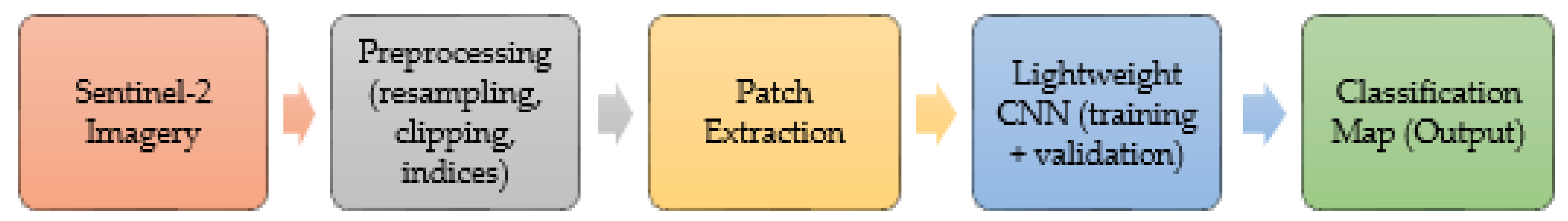
Figure 3.
Sample patches showing RGB composites (bands 4–3–2) for soil and vegetation classes. Source: Sentinel-2 (Copernicus).
Figure 3.
Sample patches showing RGB composites (bands 4–3–2) for soil and vegetation classes. Source: Sentinel-2 (Copernicus).
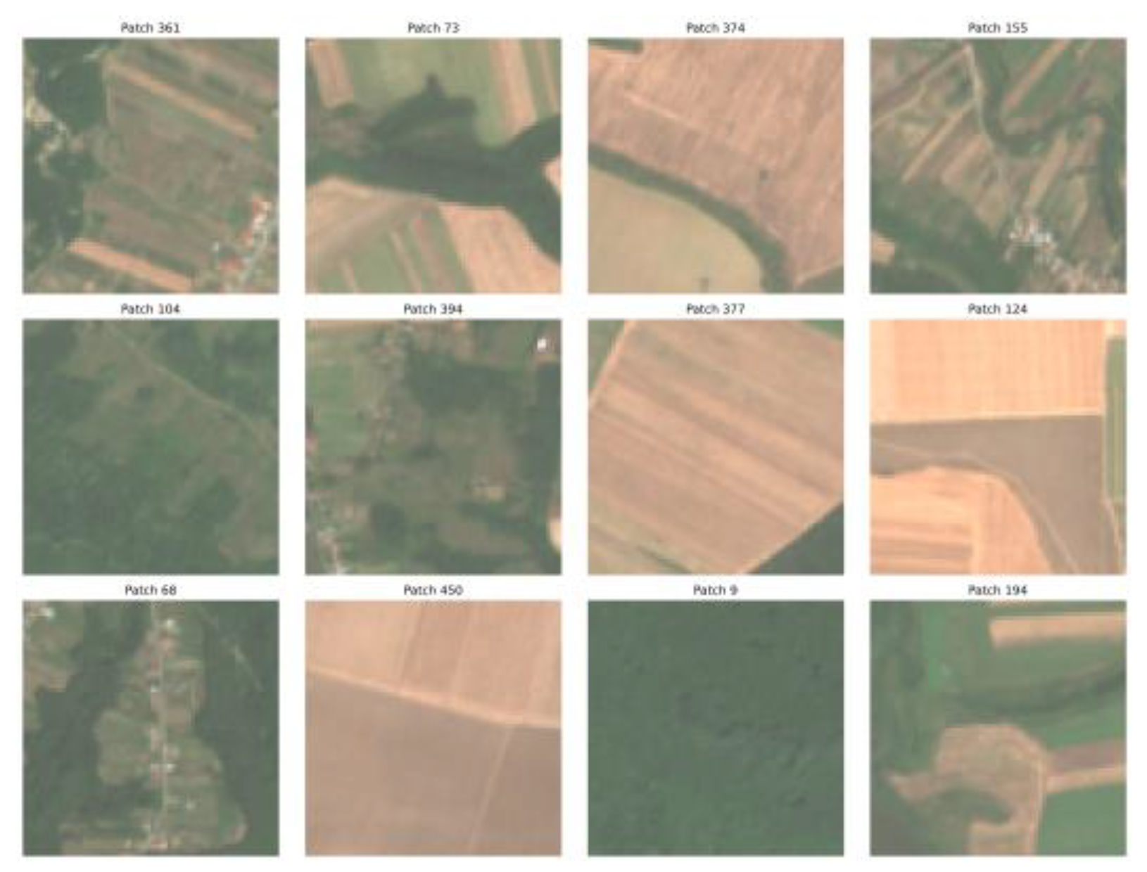
Figure 4.
Sample patches showing false-color composites (bands 8–4–3, NIR–Red–Green) for soil and vegetation classes. Vegetation is enhanced in red tones, aiding class discrimination.
Figure 4.
Sample patches showing false-color composites (bands 8–4–3, NIR–Red–Green) for soil and vegetation classes. Vegetation is enhanced in red tones, aiding class discrimination.
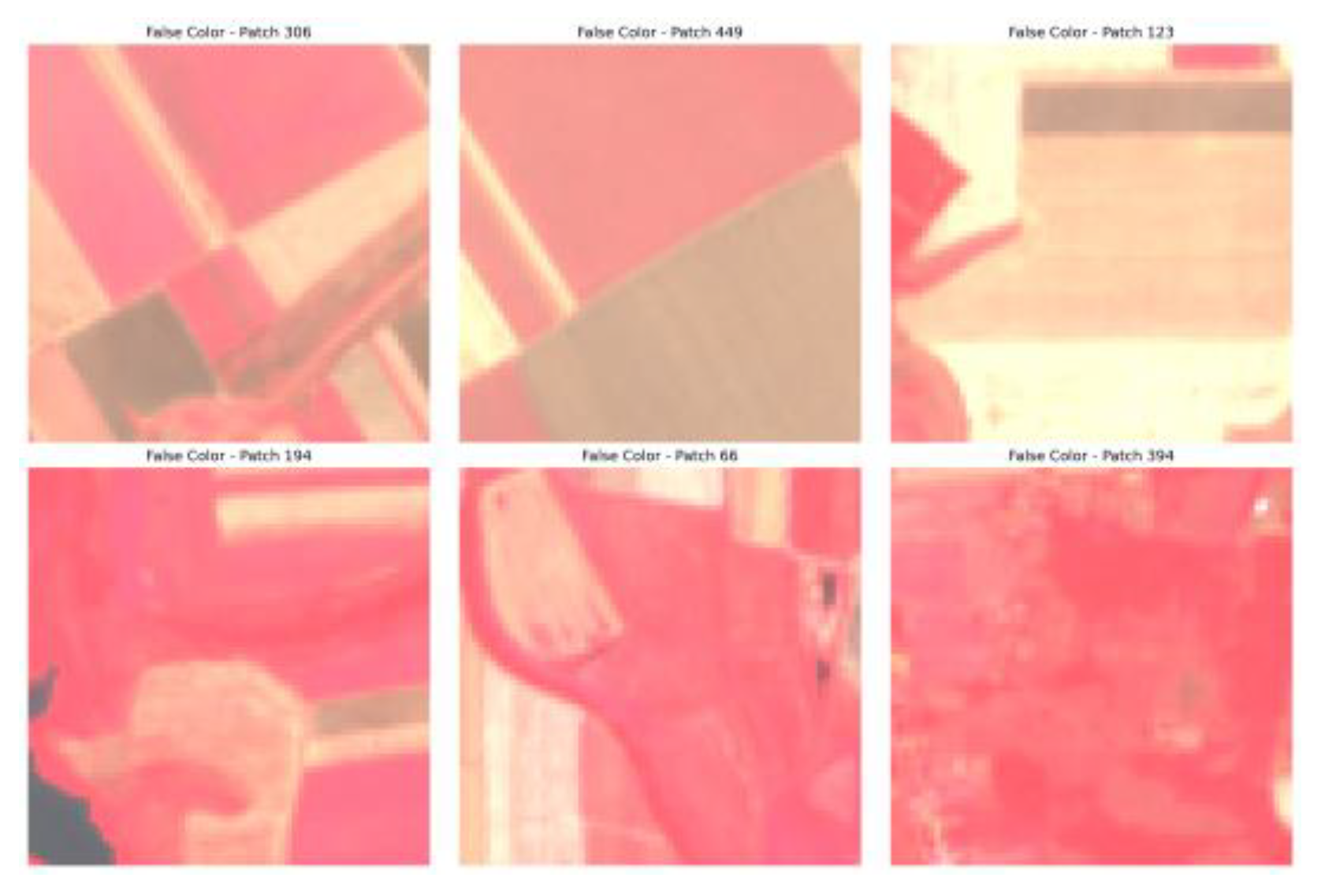
Figure 5.
Architecture of the lightweight CNN, including convolutional layers, pooling, GAP, dropout, and output classifier.
Figure 5.
Architecture of the lightweight CNN, including convolutional layers, pooling, GAP, dropout, and output classifier.
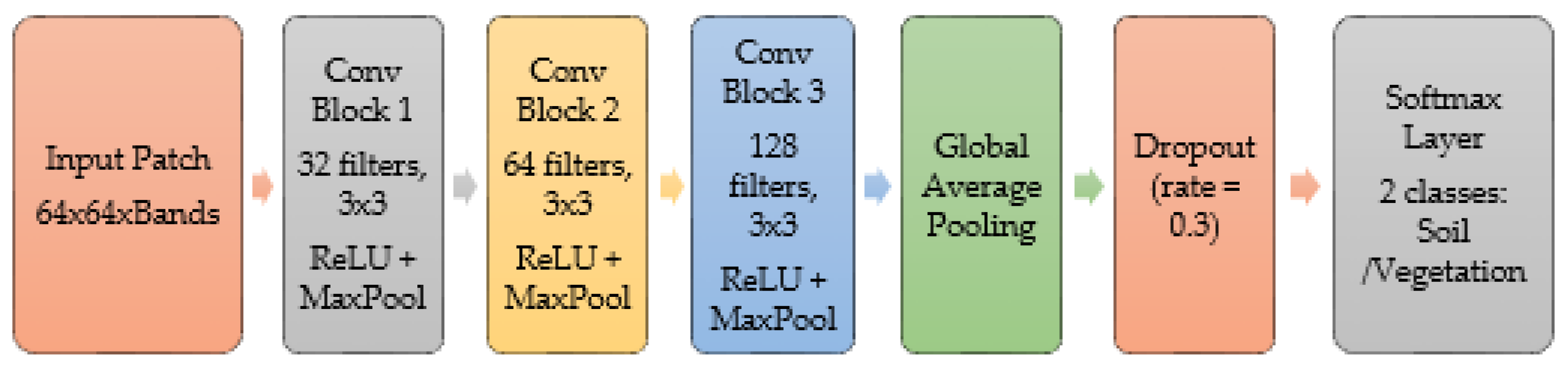
Figure 6.
NDVI distributions for correctly classified and misclassified patches. Errors concentrate in the transitional NDVI range (0.15–0.25).
Figure 6.
NDVI distributions for correctly classified and misclassified patches. Errors concentrate in the transitional NDVI range (0.15–0.25).
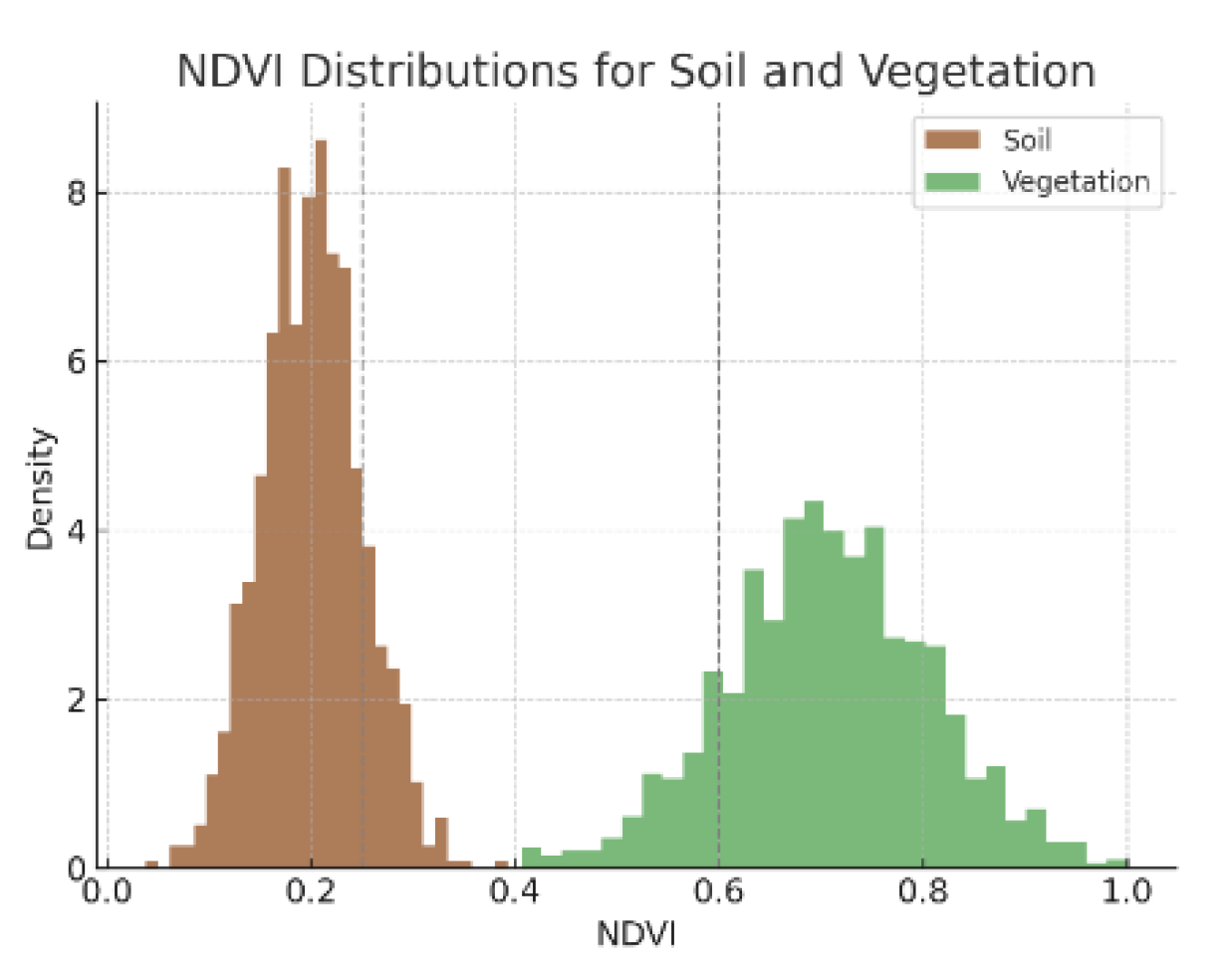
Figure 7.
Training and validation accuracy curves for the lightweight CNN. Validation accuracy stabilizes at 91.7% after ~40 epochs.
Figure 7.
Training and validation accuracy curves for the lightweight CNN. Validation accuracy stabilizes at 91.7% after ~40 epochs.
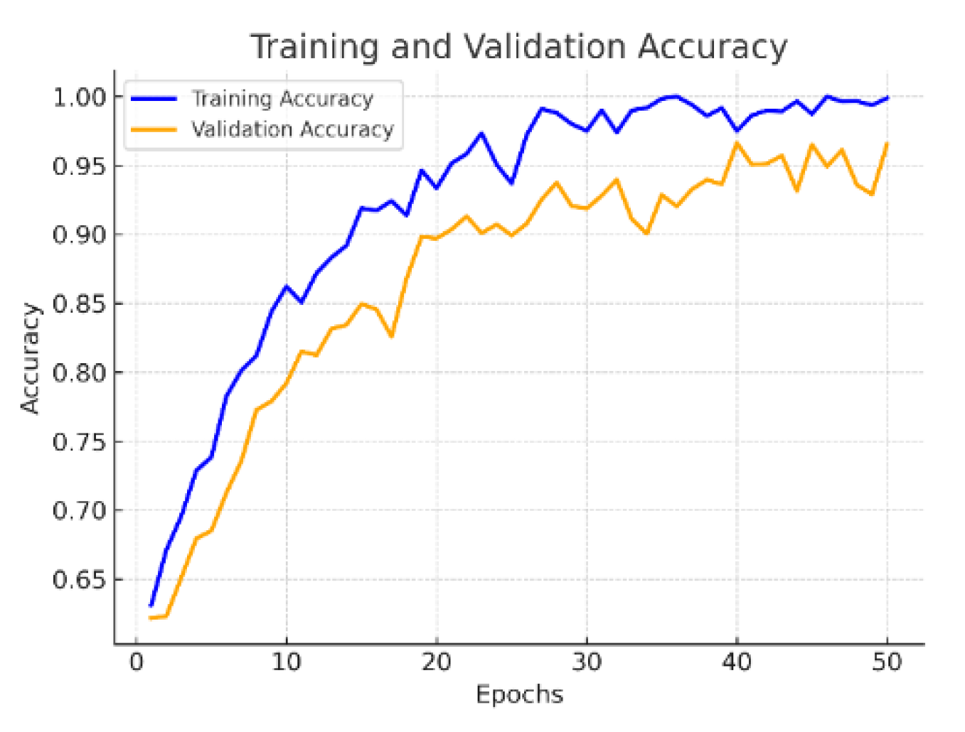
Figure 8.
Training and validation loss curves. Stable convergence and absence of divergence between curves confirm no overfitting.
Figure 8.
Training and validation loss curves. Stable convergence and absence of divergence between curves confirm no overfitting.
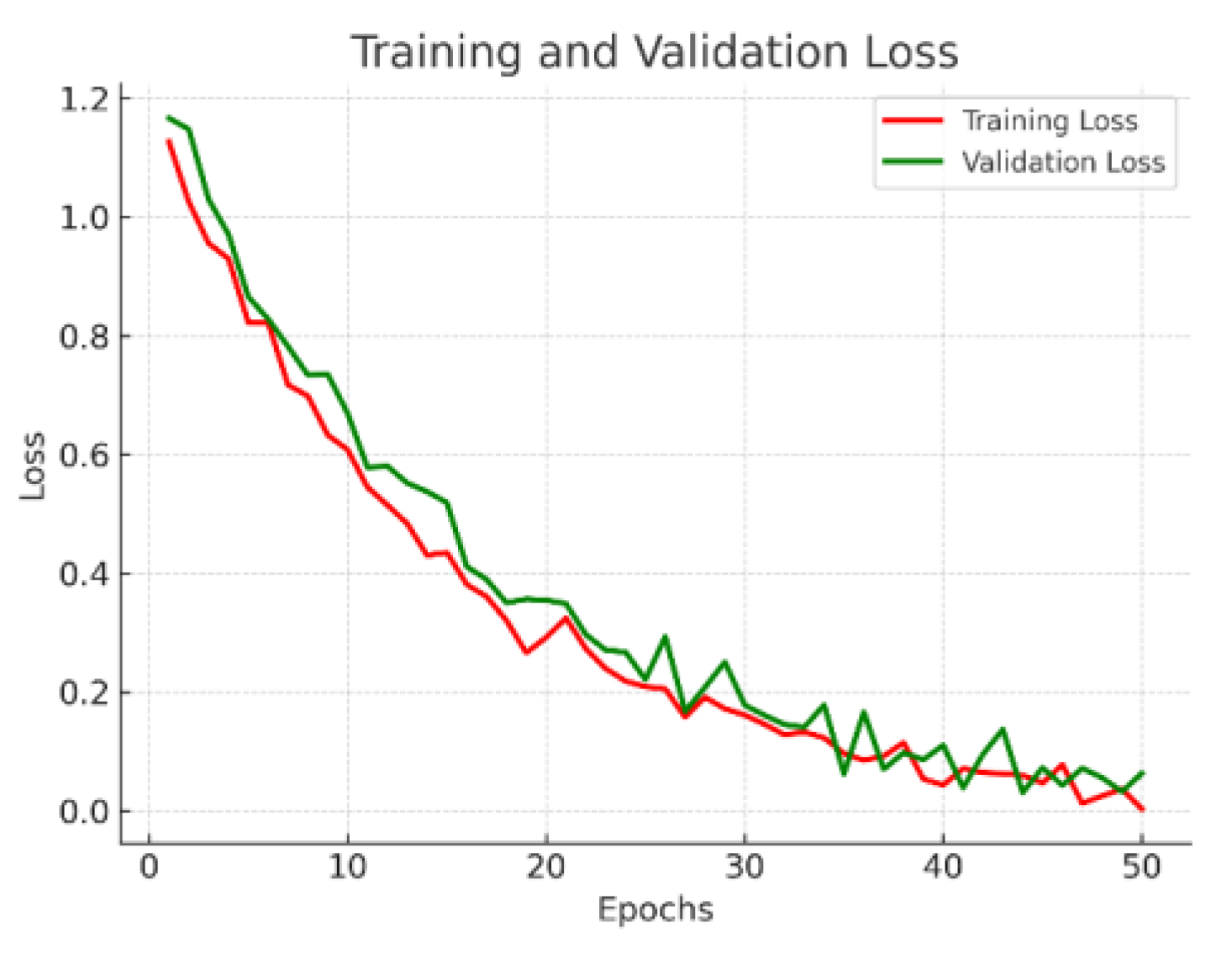
Figure 9.
Confusion matrix represented as a heatmap. The strong diagonal indicates reliable classification, while the few off-diagonal values reflect errors concentrated in transitional cases.
Figure 9.
Confusion matrix represented as a heatmap. The strong diagonal indicates reliable classification, while the few off-diagonal values reflect errors concentrated in transitional cases.
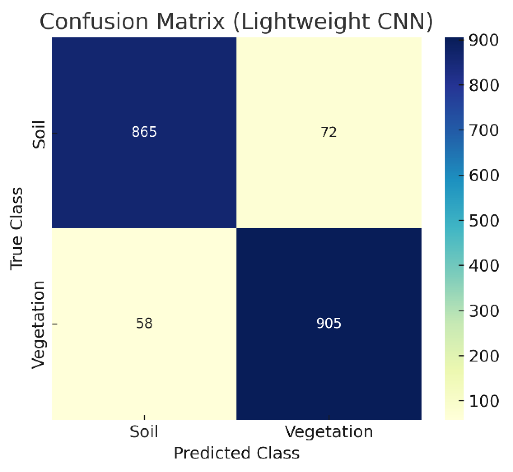
Figure 10.
Comparative overall accuracy (OA %) of the proposed lightweight CNN against NDVI baseline and representative CNN studies from the literature [8,18,31].
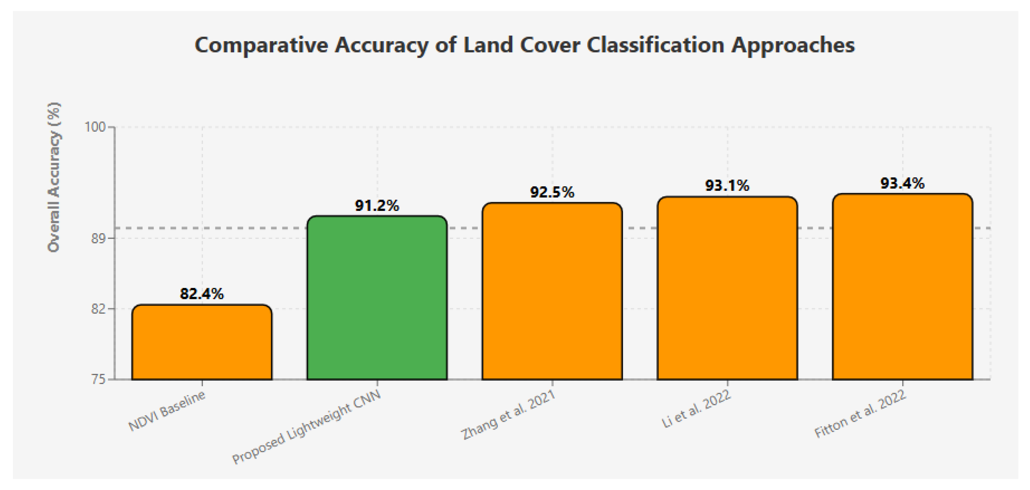
Figure 11.
Spatial classification map of Dolj County (Romania) showing soil (brown) and vegetation (green).
Figure 11.
Spatial classification map of Dolj County (Romania) showing soil (brown) and vegetation (green).
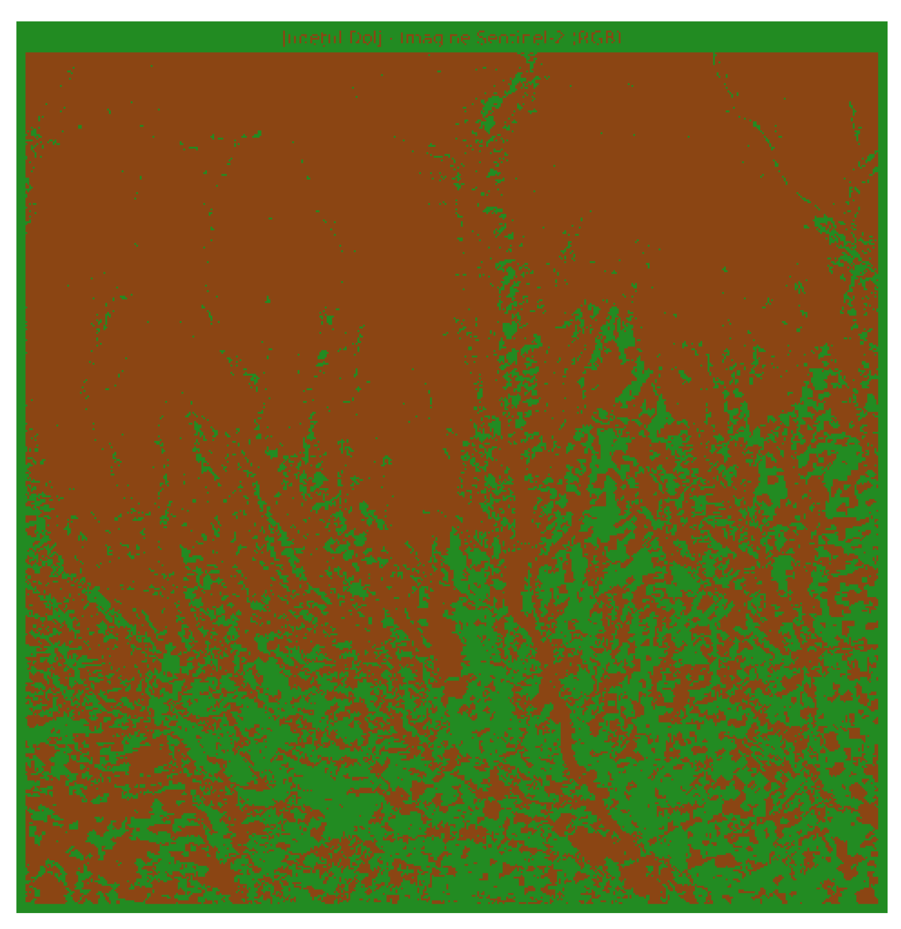

Table 1.
Sentinel-2 spectral bands used in this study, including central wavelength and spatial resolution.
Table 1.
Sentinel-2 spectral bands used in this study, including central wavelength and spatial resolution.
| Band | Wavelength (nm) | Resolution (m) | Description |
| B01 | 442.7 | 60 | Coastal aerosol |
| B02 | 492.4 | 10 | Blue |
| B03 | 559.8 | 10 | Green |
| B04 | 664.6 | 10 | Red |
| B05 | 704.1 | 20 | Red edge 1 |
| B06 | 740.5 | 20 | Red edge 2 |
| B07 | 782.8 | 20 | Red edge 3 |
| B08 | 832.8 | 10 | NIR |
| B8A | 864.7 | 20 | Red edge 4 |
| B09 | 945.1 | 60 | Water vapour |
| B11 | 1613.7 | 20 | SWIR 1 |
| B12 | 2202.4 | 20 | SWIR 2 |
Table 2.
Hyperparameters and training configuration for the lightweight CNN.
| Parameter | Value / Setting | Notes |
| Optimizer | Adam | Widely adopted in RS tasks |
| Initial learning rate | 0.001 | Stable convergence |
| Batch size | 32 | Trade-off: stability vs efficiency |
| Epochs (max) | 50 | With early stopping (patience = 10) |
| Loss function | Categorical cross-entropy | Suitable for classification tasks |
| Regularization (L2) | λ = 0.001 | Prevents overfitting |
| Dropout | 0.3 | Applied before output layer |
| Hardware | NVIDIA GTX 1660 (6 GB VRAM) | Modest GPU, reproducibility focus |
Table 3.
Overall performance metrics of the lightweight CNN model on the test set.
| Metric | Value |
| Overall Accuracy | 91.20% |
| Kappa Coefficient | 0.82 |
| Precision (macro) | 90.00% |
| Recall (macro) | 91.00% |
| F1-Score (macro) | 90.00% |
Table 4.
Class-wise performance metrics for soil and vegetation classification.
| Class | Precision | Recall | F1-Score |
| Soil | 89.00% | 88.00% | 89.00% |
| Vegetation | 91.00% | 94.00% | 92.00% |
Disclaimer/Publisher’s Note: The statements, opinions and data contained in all publications are solely those of the individual author(s) and contributor(s) and not of MDPI and/or the editor(s). MDPI and/or the editor(s) disclaim responsibility for any injury to people or property resulting from any ideas, methods, instructions or products referred to in the content. |
© 2025 by the authors. Licensee MDPI, Basel, Switzerland. This article is an open access article distributed under the terms and conditions of the Creative Commons Attribution (CC BY) license (https://creativecommons.org/licenses/by/4.0/).
Copyright: This open access article is published under a Creative Commons CC BY 4.0 license, which permit the free download, distribution, and reuse, provided that the author and preprint are cited in any reuse.


