
Submitted:
08 January 2025
Posted:
09 January 2025
You are already at the latest version
Abstract
The classification of land cover and use (LULC) is essential for territorial government, and environmental planning. Satellite images obtained in the Copernicus European program are crucial in various fields of spatial management, particularly in the conservation of cultural and natural resources. This is largely due to their wide dissemination, allowing multiple institutions and organizations to utilize them. However, their low resolution can hinder the precision of supervised AI (Artificial Intelligence) classifiers, vital for continuous land-use monitoring, especially during the training phase. This phase can be costly owing to the need for advanced technology and extensive training datasets. The research focuses on the development of an AI classifier that leverages high-resolution training data and the powerful ResNet architecture with the Benchmark for Remote Sensing Image Classification (RSI-CB128). ResNet, known for its deep residual learning capabilities, significantly enhances the classifier's ability to learn complex patterns and features from high-resolution images. A testing dataset derived from Sentinel-2 raster images is utilised to analyse the performance of the neural network (NN). Our objectives are the evaluation and full confirmation of the effectiveness of an AI classifier applied to Sentinel-2 images produced with high-definition sensors. The findings indicate substantial improvements over current classification methods, such as U-Net and OBIA, underscoring the transformative potential of ResNet in advancing land-use classification accuracy.
Keywords:
remote sensing
; convolutional neural networks
; ResNet
; object based image analysis
; neural networks
1. Introduction
The classification of land cover and use (LULC) is crucial for land governance of the territory, environmental planning, and natural resource management. In the early 1980s, the European Commission recognised the necessity for a comprehensive, meticulous, and uniform dataset regarding land use and cover across the European continent. So was launched the CORINE (Coordination of Information on the Environment) program, based on satellite images to establish a uniform methodology for producing continent-wide land cover, biotope, and air quality maps. Various satellite images have been used over time for CORINE Land Cover. The latest are Sentinel images from the satellites of the European Space Agency’s Copernicus project. Satellite imagery obtained from the Copernicus European project is essential in various fields of spatial management, particularly in the conservation of natural and cultural resources.
Copernicus imagery comprises information gathered by a constellation of satellites, optical and radar, managed by the European Space Agency (ESA) in partnership with the European Union. This constellation of satellites constitutes the foundation of the EU’s Copernicus program, offering extensive data regarding our Earth and also its processes. Copernicus data encompasses a broad spectrum of subjects, including:
- Climate and environment: Copernicus imagery is used to monitor weather conditions, land cover, climate change, quality of air and water, and biodiversity [1].
- Emergency and safety operations: Copernicus data are used to monitor hazardous human activities, including migration patterns, fishing operations, and transportation routes, as well as to track disasters, such as earthquakes, wildfires and floods [2].
- Land stewardship: Copernicus imagery is used for monitoring land use, map the territory, manage agricultural activities, natural resources, and urban development [3].
- Infrastructure and transport: Copernicus images are useful to manage ports, monitoring traffic flows, and transport infrastructure [4].
- Community health is another area where Copernicus images are used to monitor water and air quality, in addition to identifying sources of pollution [5].
Copernicus images are readily available for free via the ESA’s Open Access Hub webpage. The geometric resolution of Copernicus images is contingent upon the specific sensor employed and the rate of data collection. Optical sensors of Sentinel-2 and Sentinel-3 can capture images with resolutions between 10 and 300 meters. The protection of cultural and environmental assets can only be accomplished in an appropriate manner via the participation of a wide variety of institutions, authorities, and private individuals in the conservation and monitoring processes [6,7]. The data from the Copernicus European project serve as an essential resource; their dissemination method (complimentary and timely updates) ensures that all stakeholders involved in territorial governance can promptly identify modifications in the environment and formulate appropriate strategies in response [8]. Widespread involvement in a safety procedure is viable only if both data and analytical tools are accessible regarding cost and quality. In Figure 1 the evolution of CORINE Land Cover.
Satellite images can be categorized employing several approaches, including the Maximum Likelihood classifier, Neural Networks, Decision Trees, Support Vector Machines, and Bayes classifier [9,10]. A further distinction can be established among these between object/pixel-based classification and supervised versus unsupervised classification. Supervised classification entails the user performing the task manually, designating specific regions of the image, designated to as “training areas”, categorizing them into distinct classes, such as “forest”, “water”, or “urban area”. The classification program subsequently uses the training areas for autonomously recognizing other regions of the scene that pertain to the same category. Conversely, unsupervised classification uses algorithms for clustering to autonomously discern the many classes within the image. The categorization program examines the image and autonomously recognizes clusters of pixels with analogous characteristics, which are subsequently allocated to designated categories. The classification accuracy in both instances is contingent upon the standard of the images, the standard of the training sites, and the classification algorithms employed.
AI classifiers demonstrate exceptional performance as IT tools for analyzing Sentinel-2 images to ascertain the progression of crucial problems, like desertification [11] and coastline erosion [12], water resource availability [13], and green spaces [14]. The development of an AI classifier that incrementally integrates new categories and scenarios poses challenges for small organizations, as this process necessitates substantial amounts of training data to achieve a high-precision classifier [15], along with costly hardware and specialized technical expertise (e.g., High-Performance Computing—HPC equipment management, Field-Programmable Gate Array—FPGA, Cloud Computing). High-performance computers (HPCs) distinguish themselves from conventional computers through their specialized architecture, which includes hardware accelerators, multi-core processors, and high-speed system memory, allowing for the rapid processing of substantial data volumes. Regrettably, this may occur with Sentinel data, where inadequate spatial resolution might result in training sets compromised by labelling inaccuracies (e.g., human image classification). Neural networks are recognized for their resilience to ’noise’ [16], particularly during the training process, provided that substantial training datasets are available. Furthermore, high-resolution raster yields spectra that are semantically less confusing. The objective of this research is to examine the efficacy of an AI classifier trained using freely accessible high spatial resolution data, specifically the Remote Sensing Image Classification Benchmark [17,18]. In this particular instance, the process is tested using TensorFlow software, selecting a Convolutional (CNN) [19,20] for classification purposes, and evaluated the results also in comparison with OBIA.
2. Materials and Methods
The aim is to assess the feasibility of a successful use of AI classifiers on Sentinel-2 imagery, using an updated publicly accessible dataset composed of images with high spatial resolution. This mainly concerns environmental and cultural monitoring. The application of remote sensing facilitates the rapid and efficient acquisition of information over large areas, thereby minimizing the cost and time associated with field sampling. In addition, the accessibility of historical images facilitates the assessment of environmental changes over time and the evaluation of the effectiveness of land management policies. We evaluate the behavior and performance of a Neural Network by applying evaluation metrics and improving the performance of the proposed method. The ability to use an AI model, previously trained on high-resolution satellite datasets, capable of classifying satellite images comes in handy in various activities ranging from precision agriculture to urban planning. Among the various models capable of classifying satellite imagery we used the ResNet (Residual Network) neural network which is a convolutional neural network (CNN), renowned for its ability to train very deep networks using residual blocks. A residual block is equipped with a jump connection that bypasses one or more layers, effectively addressing the problem of evanescent gradients during training and improving the flow of information.
The use of residual blocks. In a residual block, the original input is added to the output of the layer block, creating a “skip connection”. This allows the model to learn residual functions from the original input. A residual block can be mathematically represented as:
where:
(x) is the input of the block.
(F(x, {Wi})) represents the function learned by the layer block (with parameters ({Wi})).
(y) is the output of the block.
The jump connection adds the original input (x) to the output (F(x, {W_i}), making it easier to learn residual functions.
Jump connections allow the gradient to propagate more easily through the network during the backpropagation process, reducing the problem of the gradient disappearing and improving training stability.
Thanks to residual blocks, ResNet can be trained with hundreds or even thousands of layers without compromising performance. This has enabled ResNet to achieve outstanding results in computer vision tasks such as image recognition.
There are several variants of ResNet, such as ResNet-50, ResNet-101, and ResNet-152, which differ in the number of layer. These variants have also been used in many computer vision applications, including object detection and facial recognition. ResNet-18 was used in our study.
ResNet was introduced in 2015 and won that year’s ImageNet Large Scale Visual Recognition Challenge (ILSVRC), proving its effectiveness and revolutionizing the field of deep learning The architecture consists of convolutional building blocks that are essential for feature extraction. Convolutional filters are applied to input images to identify patterns, edges, and textures. Next, normalization and activation functions are employed to extract high-level functionality. Normalization helps stabilize and speed up training, while activation functions introduce non-linearity. The architecture ends with fully connected layers, which generate predictions based on the extracted features. These layers map the learned characteristics to the final output classes. The presence of modular blocks allows ResNet to be characterized by several advantages:
- Ability to train networks with hundreds or thousands of layers: This makes it suitable for numerous deep learning applications without performance degradation.
- More efficient signal propagation: ResNet improves signal propagation both forward and backward during training.
- Excellent Performance: Produces high-quality results.
- Scalability and robustness: Its modular structure allows for easy expansion to more complex tasks while maintaining robustness and accuracy.
- Flexibility: ResNet can be used in various applications ranging from satellite imagery to facial recognition.
There exist two datasets: the RSI-CB256 dataset and the RSI-CB128 dataset RSI-CB256 is a satellite imagery dataset created to assess the efficacy of image categorization algorithms. The collection comprises satellite images obtained from multiple sources, featuring a spatial resolution of 256 × 256 pixels and 16 bits per channel. The collection has 21,061 images categorized into 45 types, encompassing trees, roads, houses, agricultural areas, water, and additional categories. The RSI-CB128 dataset comprises a collection of 36,000 images, each with a spatial resolution of 3 meters and dimensions of 128 by 128 pixels. The images were obtained in various weather conditions, seasons, and time zones, encompassing many geographical regions, including forests, agricultural lands, urban environments, and bodies of water. Every image is linked to a definitive classification map that delineates the classes contained within the image. The RSI-CB128, constructed with readily available tools (TensorFlow) and used for Sentinel-2 images, was employed to assess and compare the efficacy concerning methods for classifying remotely sensed images. For the purpose of our investigation, the dataset that contained the Sentinel-2 data was downloaded via the Kaggle platform, a website dedicated to the management for professional training sets. The catalogue is entitled EuroSat Dataset. It comprises 27,000 images at a resolution of 10 meters, with each image measuring 64x64 pixels. The bands considered are RGB, and the classifications employed are those most effective for protecting environmental assets.
In our study, the choice of images to be analyzed was made on classes useful precisely for environmental monitoring.
The selected classes were:
- Streams and reservoirs
- Marine Environment (includes coastal regions)
- Arid regions
- Verdant places
- Residential Zones
- Cultivated Fields
- Infrastructure
The selection of these categories was based on their utility in monitoring for the early identification of major issues, including coastline erosion, desertification, urban sprawl, decline of green spaces, water scarcity. They signify significant environmental issues that jeopardise the sustainability of the Earth’s ecology and the quality of human existence. These issues have enduring consequences and can inflict irreparable harm on the environment and biodiversity, in addition to exerting considerable social and economic re-percussions. Moreover, these significant challenges are frequently interrelated, and their repercussions can exacerbate one another.
Figure 2 illustrates images from the classes.
Upon defining these classes, we proceeded to the subsequent step of generating four binary files from them:
- • Training set comprised of Kaggle Sentinel-2 data (15,000 records);
- • Test set comprised of Kaggle Sentinel-2 data (1,000 records);
- • Training set comprised of RSI-CB128 data (15,000 records);
- • Test set comprised of RSI-CB128 data (1,000 records).
As a further experimental analysis, we used a second neural network to verify the validity of the methodological approach: U-Net. It is a convolutional neural network that was developed for image segmentation. The network is based on a fully convolutional neural network whose architecture was modified and extended to work with fewer training images and to yield more precise segmentation.
This network features a symmetrical U-shaped structure resulting from the mirrored paths of the contraction phase (encoder) and the expansion phase (decoder). Each layer in the encoder corresponds to a layer in the decoder, connected through skip connections. This architecture enables U-Net to effectively combine global context with local details, making it particularly powerful for image segmentation.
The encoder progressively reduces the spatial size of the input image while increasing the number of features, a process known as contraction. The encoder captures the global context of the image, which involves gathering information on a large scale. It consists of convolutional layers followed by pooling operations to extract relevant features and decrease the image resolution.
In contrast, the decoder progressively increases the spatial size of the feature maps that were reduced by the encoder, restoring them to the original resolution of the input image. This process is referred to as expansion. The decoder employs transposed convolutional layers (or upsampling) to increase resolution and reconstruct the segmented image. It also recovers local details lost during the contraction phase, aided by the skip connections.
A notable component of this architecture is the presence of skip connections that directly link the corresponding levels of the encoder and decoder. This setup allows detailed information to be transferred from the encoder to the decoder, enhancing the accuracy of the segmentation process.
2.1. Case Study
Our study area (Figure 3) is located in Italy, in the province of Reggio Calabria, encompassing the Municipality of Reggio Calabria and its constituent catchment areas, which also include parts of adjacent municipalities, up to the area of the dam on the river Menta, in a purely mountainous area.
In Figure 4 a clipping of the Sentinel true-color image of the study area, acquired on 31 May 2024.
2.1.1. Object Based Image Analysis: Segmentation
The Object Based Image Analysis is a methodology which allows a more complete image analysis than the classic pixel-based analysis, particularly with regard to satellite images. The context plays no part in the pixel-oriented analysis of satellite data, which acknowledges semantic low-level information such as the quantity of energy emitted from the pixel as its main constraint. An increase to the semantic level occurs in object-oriented analysis [21] with the addition of relation rules to the join space, topological data, statistics, and the definition of context. Mathematical morphology principles used to picture analysis and fuzzy logic components used for categorisation form the basis of recognition. In the given example, the software eCognition initially launched by Definiens Imaging GmbH, now released by Trimble, was utilised to some extent; it runs scene segmentation on many levels [22], and an experimental program is currently being examined and finalised to integrate segmentation and classification. Multiresolution segmentation [23] automatically generates vectorial polygons from the raster (which has the outstanding benefit of being superimposed on the raster with perfect coincidence) and then uses an adjusted class hierarchy that takes into consideration the relationships between the segmentation levels to perform final classification.
We analysed our study area in the province of Reggio Calabria using Object Based Image Analysis. Figure 5 illustrates the segmentation of the study area.
Beginning with objects as little as a single pixel, it is a bottom-up method for integrating regions. Subsequent processes involve merging smaller picture items into larger ones. With segment size n and a freely defined measure of heterogeneity h, the underlying optimisation algorithm minimises the weighted heterogeneity nh of the generated picture objects during the clustering process. Each stage involves merging two neighbouring picture objects, where each pair represents the minimum increase in the specified heterogeneity. This procedure terminates if even the slightest increase beyond the limit set by the scale parameter. Multiresolution segmentation does this by means of a local optimisation process.
When all of the weights from each layer are added together, the resulting spectral or colour heterogeneity is:
the variables hs, q, σc, and wc are all related to the spectral heterogeneity, the number of bands, and the weight assigned to the c spectral band, respectively.
Conversely, picture objects with a fractally shaped boundary or branched segments are the result of spectral heterogeneity minimisation strictly. Data with a lot of texture, like radar, makes this effect considerably more noticeable. To lessen the deviance from a compact or smooth shape, it is usually helpful to combine the spectral heterogeneity criterion with the spatial heterogeneity criterion. The ratio of the square root of the number of pixels making up this image object to the length of its border, l, describes heterogeneity as divergence from a compact shape.
where n is the number of pixels in the picture object, l is the border length, and hg_smooth is the fractal factor of spatial heterogeneity.
The second one is the compactness factor, which is hg_compact, and it is proportional to the polygon axis dimensional ratio:
where hg_compact is the compactness factor, l is the border length, and b is the shortest border length that can be determined by taking the bounding box of an image.
Starting with each picture pixel, the segmentation algorithm continues to fuse neighbouring polygons until the newly formed polygon’s change in observable heterogeneity falls below the customer-defined threshold (scale factor). When the change in heterogeneity is less than the stated threshold, the fusion is successful; otherwise, the two polygons stay apart. The disparity in heterogeneity (total fusion value) between the two initial polygons and the final product is:
the user-defined weight for color (versus shape) and the total fusion value (f) are both used here. Each feasible value for w falls somewhere between 0 and 1, with 1 being the most extreme case. When wf = 1, only shape heterogeneity is considered, and when wf = 0, only color heterogeneity is considered.
The spectral heterogeneity (Δhs) that differentiates the merged polygon from the two pre-merge polygons is
In this context, nmerge refers to the number of pixels in the final polygon, σmergec denotes the standard deviation of digital numbers in the c-spectral band of that polygon, nobj1 denotes the number of pixels in the first of the two polygons preceding the merge, σobj1c denotes the standard deviation of digital numbers in the c-spestral band of the first polygon preceding the merge, nobj2 = the number of pixels in the second polygon prior to the merge, and σobj2c = the standard deviation of digital numbers in the c-spestral band of the second polygon preceding the merge. To assess the impact of the merging on shape heterogeneity (Δhg), the disparity between the pre- and post-merge states is computed. Because of this, we can compute smoothness and compactness using the following methods:
(wg) is the user-defined smoothness (versus compactness) weight. When wf = 1, only smoothness is appreciated, and when wf = 0, only compactness is valued. However, any value between 0 and 1 is also acceptable for w.
The size of the resulting polygons can be adjusted by adjusting the scale factor, which is defined in relation to the cartographic scale reference that the client needs to acquire. The ability to construct hierarchical tiers of polygons with different scale factors from a single image makes the segmentation process multiresolution. Since the spectral variability intra-polygons must be smaller when the scale factor is decreased, the produced polygons get progressively smaller as the scale factor is increased. One unique aspect of multiresolution is the preexisting relationship between the polygons of the different levels of the segmentation hierarchy. It is feasible to generate n further hierarchical levels (smaller polygons) or n additional higher levels (bigger polygons) when the first level of polygons is formed, depending on the scale factor. Since lower-level hierarchical polygons always mathematically consist with higher-level ones, each lower-level polygon can only be a member of one upper-level polygon. Parameters listed in the following Table 1 take into consideration the features of an example dataset available in pan mode.
Following segmentation, the classification process will have particular characteristics.
The literature (in particular, the eCognition software developed by Definiens GmbH—founded in Munich, Germany, by Nobel Prize winner Gerd Binnig—software now released by US-based Trimble Inc.) has some knowledge of this segmentation. The aforementioned software proposes a unified package for the final classification of images that combines segmentation and Neural Fuzzy classification.
2.1.2. OBIA: Fuzzy Classification
As a mathematical method for quantifying assertions with a high degree of uncertainty, fuzzy logic uses a continuous range of [0...1] instead of the binary “yes” or “no” statements. Here, 0 indicates “exactly no” and 1 guarantees a positive answer. No value between zero and one is less definitive than a yes or no.
The use of fuzzy sets for land terrain cover classification is rather recent compared to classical classification techniques [24]. A better approach to this issue can be found in fuzzy sets theory, which was developed to handle imperfect data [25,26,27,28,29,30]. The principles and methods it offers are really helpful for dealing with vague data. Each area might become partially or fully enrolled in various classes. The degree to which a region’s features resemble a given class is shown by its membership grade function with regard to that class. The membership grade can have a value between zero and one. More area falls into that category when the value gets closer to 1. Cover mixture and intermediate conditions are examples of more complicated circumstances that can benefit from partial membership.
Fuzzy logic simulates human cognition and incorporates linguistic principles.
For the most part, fuzzy classification systems can handle ambiguity when it comes to extracting data from remote sensing. The use of membership functions to build fuzzy sets allows for the consideration of parameter and model uncertainties. Instead than just having two possible outcomes, multivalued fuzzy logic lets you choose between “true” and “false” as values.
The logical operators “and” and “or” have more or less rigid realisations.
When a fuzzy classification system is run, the result is a fuzzy classification that assigns each object a membership degree to a specific land use or cover class. Because of this, we can examine the class mixture for each picture object and do in-depth analyses of their performance. Soft classification has this huge benefit. The ultimate categorisation for creating an interface to sharp systems is determined by the maximum membership degree.
In Figure 6, using the feature x, define the crisp set M (green) μM(X) and the fuzzy set A (yellow) μA(X) across the feature range X using rectangular and trapezoidal membership functions.
In Figure 7, feature x’s membership functions define Fuzzy ranked this feature as low, medium, or high.
In Figure 8, fuzzy classification for the specified land cover categories: urban, water, and vegetation. The image object is a a member of every class to varying degrees:
Figure 9 shows the fuzzy classification of the three land cover types that were considered: urban, water, and vegetation. When the membership degrees of the two classes are equal, it means that the object in the picture is unstablely classified between them. If the land cover classes are typically distinguishable in the dataset, then this finding suggests that all land cover classes are present within the picture object to a comparable extent. The elevated membership value indicates that the allocation to this class mixture is reliable.
As shown in Figure 10, the considered image objects unstable classification between these classes is further indicated by the equal membership degrees. Nevertheless, the assignment is extremely unreliable because of the low membership value. No class assignment will be provided in the final output if the minimal membership degree is 0.3.
Differentiating structural methodology from traditional spectrum analysis include object-based classification and multiresolution segmentation methods. As the resolution of remote sensing images improves, the statistical definition with pixel-based analysis of land use groups increases ambiguity. Instead, we can use object-based analysis to get better data from remote sensing, which is immediately usable in GIS and lets make vector maps. Were applied concepts from mathematical morphology and fuzzy logic, organises data hierarchically, and agrees to arrange different typologies, all while integrating raster and vectorial data. The automatic ability to recognise things on land is enhanced by the introduction of rules for context localisation and meaningful object relations. This methodology, which is based on the same principles as manual photointerpretation, solves the issues with traditional classification methods by creating a reproducible and consistent process, thereby going beyond the limitations of subjective classification.
2.2.1. Processing Phases
The methodological approach required the following steps (Figure 11).
- Understanding Sentinel Image Classification: The task involved labeling images taken from satellites (Sentinel) into categories like forest, water, urban area, etc.
- Data collection and image editing in similar sizes.
- Preprocessing the Data: Resizing Images, all images were resized to ensure they were of the same size; normalizing Pixel Values, the pixel values were scaled between 0 and 1 for better model performance; transformations data, rotations, flips, or zooms were applied to increase the variety in the dataset tag. This step in the process significantly improves the performance of the model. Isaac Corley et al. [31] in fact in their paper explore the importance of image size and normalization in pre-trained models for remote sensing.
- Choosing a Model: A model like a Convolutional Neural Network (CNN) was selected initially. The retrained models like ResNet were considered for better accuracy, as it already knows how to identify general features.
- Training the Model: The dataset was divided into training and testing sets.
Network architecture: It consists of 18 convolutional layers distributed as follows, 1 initial (7x7), 2 for each residual block (8 in total), 4 for the skip connections, 2 for each transition level (4 in total), 1 final (1x1). Dense layers, 2 for each attention block (4 attention blocks) in total 8. ReLU layers, 1 after each convolutional layer (18 convolutional layers) total 18.
The main functions of the network are:
- Network typology: It uses “skip” (residual) connections that simplify training. These connections help mitigate the problem of gradient disappearance, allowing for stronger gradients and better stability during training.
- Performance on images: It shows good performance on image classification datasets. Its residual block architecture allows to better capture the characteristics of complex images.
- Generalization: Because of its depth and residual connections, tends to generalize well to test datasets.
- Dataset: The dataset that maps the image names with the respective tags (labels) is read and modified. Additionally, another column that includes the respective labels as list items is created. Using that column, we extracted the unique labels existing at the dataset [32].
- Image Caption approach with visual attention: The attention mechanism has been applied to improve performance [33]. It is a mechanism that allows deep learning models to focus on specific parts of an image that are most relevant to the task at hand, while ignoring less important information.
The model generates an attention map that highlights the areas of the image that contain crucial information. Each pixel or region of the image receives a weight that indicates its relative importance. These weights are learned during the training process. This function is also found in other networks used for remote sensing image classification such as RNN (Recurrent Neural Network) [34].
From this comparison, the following assessment emerges: the method works, and the analysis conducted is comparable if not significantly better than OBIA: with OBIA the overall accuracy was 90.6%.
In Figure 12 a classification, derived with OBIA from Sentinel-2 dataset, in eight ecotypes
4. Results
After the preprocessing phase, training was carried out, followed by the validation phase. Once the training and validation phases are finished for ResNet, the following results were obtained: a Loss value of 0.291544 and an accuracy value of 0.93. These results confirm that the model is able to correctly classify satellite images. Figure 13 shows the loss diagram.
To evaluate the reliability of the System, a test was carried out on Sentinel-2 images referring to the area of study. At the end of the processing to evaluate the validity of the model, the following metrics were derived at the end of 69 epochs:
Accuracy: 0.96.
Precision: 0.92.
Recall: 0.85.
F1-score: 0.82.
The Loss diagram (Figure 14) shows a value of 0.1334. Low values indicate that the model is learning well from the data provided.
The ROC/AUC curve (Figure 15) shows a value of: 0.89. Its value is very good and indicates that the model is effective in distinguishing between positive and negative classes.
The results obtained confirm the validity of the proposed method for the classification of satellite images.
As a further experimental analysis, we used the second neural network to verify the validity of the methodological approach. The same data were given as input to U-Net network.
The metrics obtained with this network were:
Accuracy: 0.83
Precision: 0.71
Recall: 0.79
F1-score: 0.70
Figure 16 shows the ROC/AUC curve of the U-Net network.
In the context of classifying satellite imagery, it is critical to evaluate the performance of the neural network models used. In this comparison, we analyze the metrics of two popular neural networks: ResNet and U-Net, to determine which model performs better and in which aspects each excels.
The ROC/AUC curve for ResNet shows a value of 0.89, while for U-Net it is 0.69. This indicates that ResNet has a higher discrimination capacity than U-Net. In terms of accuracy, ResNet achieved a value of 0.96, indicating that the model correctly classified 96% of the images, compared to 83% for U-Net. This suggests that ResNet is much more accurate overall. As far as precision is concerned, ResNet has a value of 0.92, which means that 92% of images classified as positive are actually positive. U-Net, on the other hand, has an accuracy of 0.71, suggesting a higher presence of false positives than ResNet. Analyzing recall, ResNet has a value of 0.85, indicating that 85% of positive images were correctly identified, while U-Net has a recall of 0.79. This is a good result for U-Net, but still lower than ResNet. The F1-score, which represents the harmonic average of precision and recall, is 0.82 for ResNet, indicating a good balance between these two metrics. U-Net, on the other hand, has an F1-score of 0.70, suggesting that there is room for improvement to balance accuracy and recall.
These results clearly show that the performance of the ResNet network is generally superior to that of the U-Net network. Not only does ResNet offer greater accuracy and precision, but it is also more effective at reducing false negatives. Furthermore, comparing the accuracy value obtained with the OBIA method (the overall accuracy of OBIA was 90.6 %), it was found that it is comparable with the ResNet network. This suggests that ResNet is a more powerful and reliable choice for classifying Sentinel-2 images.
5. Discussion
In our work, we applied the ResNet network with the attention mechanism to improve the classification of Sentinel-2 images. The choice of ResNet was motivated by its ability to handle deep networks without running into the problem of gradient disappearance, while the attention mechanism allowed the analysis to focus on the relevant characteristics of the images, further improving accuracy. The results obtained show a marked improvement compared to the methodologies currently employed, highlighting how the use of high-resolution training data can compensate for the inherent limitations of Sentinel-2 data. In addition, the proposed approach demonstrates increased computational efficiency, reducing the costs associated with training complex models. This makes our methodology particularly useful for practical applications in the field of environmental monitoring, where accuracy and efficiency are critical. The results suggest that the integration of advanced neural networks with attention mechanisms represents a promising direction for research and future applications in the field of remote sensing.
The choice of this methodological approach was the result of a series of evaluations that highlight its innovative aspect.
RSI-CB128 is a broad and diverse benchmark, based on crowdsourced data, covering many land use categories. Training ResNet on this dataset improves the model’s ability to generalize to non-visible data, such as Sentinel-2, increasing the robustness of the model. In addition, using a pre-trained model on RSI-CB128 and then refining it on Sentinel-2 data allows you to transfer knowledge learned from a large and diverse dataset into a specific context. As a result, this approach can improve model performance on Sentinel-2 specific data.
Another important aspect is that ResNet is known for its efficiency in managing deep networks thanks to residual blocks. This can be especially useful when working with large datasets such as RSI-CB128 and Sentinel-2, reducing training and inference time. In addition, the use of crowdsourced data to build the RSI-CB128 benchmark is an innovative approach that leverages the vast amount of data available online. Thanks to this method, the benchmark can continue to expand in terms of diversity and sample quantity, continuously improving the model.
The combination of these elements, a robust model such as ResNet with a diversified benchmark such as RSI-CB128 and high-resolution data such as Sentinel-2, can lead to significant practical applications in various fields, such as precision agriculture, natural resource management and environmental monitoring.
Offering unique advantages over other models, comparing ResNet with other neural networks commonly used for classifying satellite imagery highlights several aspects that support the choice made. In terms of accuracy, ResNet stands out for its high precision, thanks to residual blocks that allow very deep networks to be trained without evanescent gradient problems. However, this accuracy comes at a cost in terms of computational efficiency, as ResNet requires significant resources and longer training times. As for sturdiness, ResNet is good, but it may be less robust than newer models like the Transformers.
On the other hand, U-Net is excellent for image segmentation, although it may be less effective for pure classification than ResNet. U-Net offers a good balance between accuracy and resource requirements, making it moderately computationally efficient. Its robustness is particularly good for segmentation tasks.
EfficientNet, on the other hand, offers an excellent balance between accuracy and computational efficiency. Thanks to the optimized scalability of the network, EfficientNet is very computationally efficient. However, for best results, it may require accurate setup. Its robustness is good, but as with other models, it depends on the configuration.
DenseNet promotes the reuse of learned features, which contributes to its high accuracy. However, this network can be more complex and require more computational resources than ResNet. The robustness of DenseNet is good, but the density of the connections can increase the complexity of the model.
Finally, Vision Transformers (ViT) exhibit high levels of accuracy, with pre-trained models such as MobileViTV2 and EfficientViT-M2 demonstrating excellent performance. However, ResNet can make it easier to interpret the results and diagnose any issues. In terms of computational efficiency, ViTs are more efficient in terms of power consumption and inference time than ResNet. However, ResNet may perform better on specific datasets or in contexts where the data is similar to what it was pre-trained on.
In addition, the comparison of metrics between ResNet and U-Net showed that the former performs better, confirming ResNet’s choice for satellite image classification tasks.
Among the innovative aspects of ResNet, one of the most relevant is the depth of the network. Thanks to its deep networks, ResNet is able to capture complex and detailed features from satellite imagery, improving classification accuracy compared to shallower networks. Another key element is residual learning. The ResNet framework utilizes the concept of residual learning, which facilitates the training of very deep networks while reducing the problem of gradient degradation. This is particularly useful for managing the complexity of Sentinel-2 imagery.
The application to multispectral data is another strength of ResNet. Sentinel-2 images are multispectral, and ResNet can be adapted to take advantage of these different spectral bands, improving the ability to distinguish between different classes of land cover. Using a benchmark such as the RSI-CB128 for training provides a standardized and well-annotated dataset, which helps to evaluate and compare model performance more rigorously.
Innovations in image pre-processing are an additional advantage. The integration of advanced pre-processing techniques, such as atmospheric correction and cloud removal, can further improve the quality of input images, making classification more accurate.
The image pre-processing phase allows you to improve the quality of the data and prepare it for analysis. In particular, atmospheric correction removes atmospheric effects (such as light absorption and scattering) to achieve more accurate reflectance values. Cloud removal uses masking algorithms to identify and remove areas covered by clouds. Geometric rectification aligns images to a standard geographic grid, correcting for any geometric distortions caused by the satellite’s acquisition angle. Resampling standardizes all bands to a common resolution, usually 10m, to facilitate analysis. Reducing resolution and selecting subsets reduces data volume and processing time by selecting only the relevant bands and areas of interest. Finally, images are often converted to more manageable formats, such as GeoTIFF.
The results obtained indicate that the adoption of neural networks trained with high-resolution data can mitigate some of the problems related to low resolution, improving the accuracy of predictions. For the future, further improvements could come from the use of data with different spatial and temporal resolutions and the optimization of the preprocessing phase. In addition, it will be crucial to develop algorithms that can adapt to environmental variations and handle complex data, thus ensuring greater robustness and accuracy in predictive models.
6. Conclusions
The Sentinel data and Copernicus project are critically important for the ongoing surveillance of the terrain to safeguard cultural and environmental assets. Thus, we established both alert and long-term mitigation systems.
The project’s numerous benefits are especially highlighted by the proposed data access method, which enables various organizations and associations with constrained budgets to conduct successful analyses using their informational content.
Conversely, the current solutions may necessitate the utilization of costly proprietary tools to attain effective classifications. This study proposed the application of ResNet classifier, trained on publicly available high spatial resolution datasets, for analysis of Sentinel data. From the comparison made, the following assessment emerges: the method works, and the analysis conducted is finally comparable to OBIA. This assessment is important because the software for OBIA is currently a proprietary software.
The comparison also showed that while the OBIA method is comparable, it is not preferable to Neural Network as the latter has the following advantages:
- Generalisation Capability: ResNet is able to learn more complex representations and generalise better to new data than traditional methods such as OBIA, which often require manual segmentation and may be less flexible.
- Automation and Scalability: The use of ResNet allows for high automation in the classification process, reducing the need for manual intervention. This is particularly useful for analysing large volumes of satellite data, where efficiency and scalability are crucial.
- Robustance to Noisy Data: Deep neural networks, including ResNet, tend to be more robust to noisy data and image variations, improving classification accuracy compared to segmentation-based methods such as OBIA.
- Integration of Multispectral Information: ResNet can easily integrate information from different spectral bands, further improving the classification accuracy of satellite images.
The proposed method allows various associations and organizations with limited budgets to carry out successful analyses using their information content, without having to resort to expensive proprietary software.
The aim of this study was to test an AI classifier of Sentinel2 images from high-resolution Remote Sensing Image Classification Benchmark (RSI-CB128) training data. After the training phase on data obtained from high-resolution images, the network was tested on data referring to images relating to specific areas of the territory. The results obtained have shown that the type of network adopted shows better performance than the methodologies in use.
This approach not only increases accuracy, but also reduces the need for extensive training datasets and advanced hardware, making the technology more accessible and less expensive for environmental monitoring applications.
As a future development to improve image classification through the ResNet net-work, it is possible to intervene on the use of more data by resorting to images with different spatial and temporal resolutions. Still improving the preprocessing phase, developing new algorithms aimed at improving accuracy. Finally, verify the network’s ability to learn complex data and adapt to environmental variations.
Author Contributions
Conceptualization, G.B., L.B., G.M.M., E.G. and V.B.; methodology, G.B., L.B., G.M.M., E.G. and V.B.; software, G.B., L.B., G.M.M., E.G. and V.B.; validation, G.B., L.B., G.M.M., E.G. and V.B.; formal analysis, G.B., L.B., G.M.M., E.G. and V.B.; investigation, G.B., L.B., G.M.M., E.G. and V.B.; resources, G.B., L.B., G.M.M., E.G. and V.B.; data curation, G.B., L.B., G.M.M., E.G. and V.B.; writing—original draft preparation, G.B., L.B., G.M.M., E.G. and V.B.; writing—review and editing, G.B., L.B., G.M.M., E.G. and V.B.; visualization, G.B., L.B., G.M.M., E.G. and V.B.; supervision, G.B., L.B., G.M.M., E.G. and V.B.; project administration, G.B., L.B., G.M.M., E.G. and V.B. All authors have read and agreed to the published version of the manuscript.
Funding
This research received no external funding.
Data Availability Statement
Not applicable.
Acknowledgments
The contribution is the result of ongoing research under the PNRR National Recovery and Resilience Plan, Mission 4 “Education and Research,” funded by Next Generation EU, within the Innovation Ecosystem project “Tech4You” Technologies for climate change adaptation and quality of life improvement,- SPOKE 4- Technologies for resilient and accessible cultural and natural heritage, Goal 4.6 Planning for Climate Change to boost cultural and natural heritage: demand-oriented ecosystem services based on enabling ICT and AI technologies.
Conflicts of Interest
The authors declare no conflict of interest.
References
- Buontempo, C.; Hutjes, R.; Beavis, P.; Berckmans, J.; Cagnazzo, C.; Vamborg, F.; Thépaut, J.N.; Bergeron, C.; Almond, S.; Amici, A.; Dee, D. Fostering the development of climate services through Copernicus Climate Change Service (C3S) for agriculture applications. Weather and Climate Extremes 2020, 27, 100226. [Google Scholar] [CrossRef]
- Ajmar, A.; Boccardo, P.; Broglia, M.; Kucera, J.; Giulio-Tonolo, F.; Wania, A. Response to flood events: The role of satellite-based emergency mapping and the experience of the Copernicus emergency management service. Flood damage survey and assessment: New insights from research and practice 2017, 211–228. [Google Scholar]
- Pace, R.; Chiocchini, F.; Sarti, M.; Endreny, T.A.; Calfapietra, C.; Ciolfi, M. Integrating Copernicus land cover data into the i-Tree Cool Air model to evaluate and map urban heat mitigation by tree cover. European Journal of Remote Sensing 2023, 56, 2125833. [Google Scholar] [CrossRef]
- Soulie, A.; Granier, C.; Darras, S.; Zilbermann, N.; Doumbia, T.; Guevara, M.; Jalkanen, J.P.; Keita, S.; Liousse, C.; Crippa, M.; Smith, S. Global anthropogenic emissions (CAMS-GLOB-ANT) for the Copernicus Atmosphere Monitoring Service simulations of air quality forecasts and reanalyses. Earth System Science Data Discussions 2023, 1–45. [Google Scholar] [CrossRef]
- Chrysoulakis, N.; Ludlow, D.; Mitraka, Z.; Somarakis, G.; Khan, Z.; Lauwaet, D.; Hooyberghs, H.; Feliu, E.; Navarro, D.; Feigenwinter, C.; Holt Andersen, B. Copernicus for urban resilience in Europe. Scientific Reports 2023, 13, 16251. [Google Scholar] [CrossRef]
- Barrile, V.; Bilotta, G. Fast extraction of roads for emergencies with segmentation of satellite imagery. Procedia Soc. Behav. Sci. 2016, 223, 903–908. [Google Scholar] [CrossRef]
- Bilotta, G.; Calcagno, S.; Bonfa, S. Wildfires: an Application of Remote Sensing and OBIA. WSEAS Trans. Environ. Dev. 2021, 17, 282–296. [Google Scholar] [CrossRef]
- Salgueiro, L.; Marcello, J.; Vilaplana, V. Single-Image Super-Resolution of Sentinel-2 Low Resolution Bands with Residual Dense Convolutional Neural Networks. Remote Sens. 2021, 13, 5007. [Google Scholar] [CrossRef]
- Fotso Kamga, G.A.; Bitjoka, L.; Akram, T.; Mengue Mbom, A.; Rameez Naqvi, S.; Bouroubi, Y. Advancements in satellite image classification: methodologies, techniques, approaches and applications. International Journal of Remote Sensing 2021, 42, 7662–7722. [Google Scholar] [CrossRef]
- Ben Hamida, A.; Benoit, A.; Lambert, P.; Ben Amar, C. 3-D Deep Learning Approach for Remote Sensing Image Classification. IEEE Trans. Geosci. Remote Sens. 2018, 56, 4420–4434. [Google Scholar] [CrossRef]
- Ren, Y.; Zhang, B.; Chen, X.; Liu, X. Analysis of spatial-temporal patterns and driving mechanisms of land desertification in China. Science of The Total Environment 2024, 909, 168429. [Google Scholar] [CrossRef] [PubMed]
- Samaei, S.R.; Ghahfarrokhi, M.A. AI-Enhanced GIS Solutions for Sustainable Coastal Management: Navigating Erosion Prediction and Infrastructure Resilience. In Proceedings of the 2nd International Conference on Creative achievements of architecture, urban planning, civil engineering and environment in the sustainable development of the Middle East; 2023. [Google Scholar]
- Kamyab, H.; Khademi, T.; Chelliapan, S.; SaberiKamarposhti, M.; Rezania, S.; Yusuf, M.; Farajnezhad, M.; Abbas, M.; Jeon, B.H.; Ahn, Y. The latest innovative avenues for the utilization of artificial Intelligence and big data analytics in water resource management. Results in Engineering 2023, 101566. [Google Scholar] [CrossRef]
- Farkas, J.Z.; Hoyk, E.; de Morais, M.B.; Csomós, G. A systematic review of urban green space research over the last 30 years: A bibliometric analysis. Heliyon 2023, 9. [Google Scholar] [CrossRef]
- Adegun, A.A.; Viriri, S.; Tapamo, J.R. Review of deep learning methods for remote sensing satellite images classification: experimental survey and comparative analysis. Journal of Big Data 2023, 10, 93. [Google Scholar] [CrossRef]
- Ding, Y.; Cheng, Y.; Cheng, X.; Li, B.; You, X.; Yuan, X. Noise-resistant network: a deep-learning method for face recognition under noise. J Image Video Proc. 2017, 43. [Google Scholar] [CrossRef]
- Li, H.; Dou, X.; Tao, C.; Wu, Z.; Chen, J.; Peng, J.; Deng, M.; Zhao, L. RSI-CB: A Large-Scale Remote Sensing Image Classification Benchmark Using Crowdsourced Data. Sensors 2020, 20, 1594. [Google Scholar] [CrossRef] [PubMed]
- Helber, P.; Bischke, B.; Dengel, A.; Borth, D. Eurosat: A novel dataset and deep learning benchmark for land use and land cover classification. IEEE Journal of Selected Topics in Applied Earth Observations and Remote Sensing 2019, 12, 2217–2226. [Google Scholar] [CrossRef]
- Simonyan, K.; Zisserman, A. Very Deep Convolutional Networks for Large Scale Visual Recognition. arXiv 2014. [Google Scholar] [CrossRef]
- Szegedy, C.; Liu, W.; Jia, Y.; Sermanet, P.; Reed, S.; Anguelov, D.; Erhan, D.; Vanhoucke, V.; Rabinovich, A. Going deeper with convolutions. arXiv 2014. [Google Scholar] [CrossRef]
- Benediktsson, J.A.; Pesaresi, M.; Arnason, K. Classification and Feature Extraction for Remote Sensing Images from Urban Areas Based on Morphological Transformations. IEEE Transactions on Geoscience and Remote Sensing 2003, 41, 1940–1949. [Google Scholar] [CrossRef]
- Baatz, M.; Benz, U.; Dehgani, S.; Heynen, M.; Höltje, A.; Hofmann, P.; Lingenfelder, I.; Mimler, M.; Sohlbach, M.; Weber, M.; Willhauck, G. eCognition 4.0 professional user guide; Definiens Imaging GmbH: München, 2004. [Google Scholar]
- Köppen, M.; Ruiz-del-Solar, J.; Soille, P. Texture Segmentation by biologically-inspired use of Neural Networks and Mathematical Morphology. In Proceedings of the International ICSC/IFAC Symposium on Neural Computation (NC’98); ICSC Academic Press: Vienna, 1998; pp. 23–25. [Google Scholar]
- Pesaresi, M.; Kanellopoulos, J. Morphological Based Segmentation and Very High Resolution Remotely Sensed Data, in Detection of Urban Features Using Morphological Based Segmentation, MAVIRIC Workshop, Kingston University, 1998.
- Serra, J. Image Analysis and Mathematical Morphology; 2, Theoretical Advances; Academic Press: New York, 1998. [Google Scholar]
- Shackelford, A.K.; Davis, C.H. A Hierarchical Fuzzy Classification Approach for High Resolution Multispectral Data Over Urban Areas. IEEE Transactions on Geoscience and Remote Sensing 2003, 41, 1920–1932. [Google Scholar] [CrossRef]
- Small, C. Multiresolution Analysis of Urban Reflectance, IEEE/ISPRS joint Workshop on Remote Sensing and Data Fusion over Urban Areas, Rome, 2001.
- Soille, P.; Pesaresi, M. Advances in Mathematical Morphology Applied to Geoscience and Remote Sensing. IEEE Transactions on Geoscience and Remote Sensing 2002, 41, 2042–2055. [Google Scholar] [CrossRef]
- Tzeng, Y.C.; Chen, K.S. A Fuzzy Neural Network to SAR Image Classification. IEEE Transaction on Geoscience and Remote Sensing 1998, 36, 301–307. [Google Scholar] [CrossRef]
- Zadeh, L.A. Fuzzy Sets. Information Control 1965, 8, 338–353. [Google Scholar] [CrossRef]
- Addabbo, P.; Focareta, M.; Marcuccio, S.; Votto, S.; Ullo, S.L. Contribution of Sentinel-2 data for applications in vegetation monitoring. Acta Imeko. 2016, 5, 44–54. [Google Scholar] [CrossRef]
- Bilotta, G. OBIA to Detect Asbestos-Containing Roofs. In International Symposium: New Metropolitan Perspectives; 2022; pp. 2054–2064. [Google Scholar]
- Corley, I.; Robinson, C.; Dodhia, R.; Lavista Ferres, J.M.; Najafirad, P. Revisiting pre-trained remote sensing model bench-marks: resizing and normalization matters. arXiv 2023. [Google Scholar] [CrossRef]
- https://www.tensorflow.org/tutorials/text/image_captioning.
- Bos, T.; Schmidt-Hieber, J. Convergence rates of deep ReLU networks for multiclass classification. Electronic Journal of Statistics 2022, 16, 2724–2773. [Google Scholar] [CrossRef]
- Ghaffarian, S.; Valente, J.; van der Voort, M.; Tekinerdogan, B. Effect of Attention Mechanism in Deep Learning-Based Remote Sensing Image Processing: A Systematic Literature Review. Remote Sens. 2021, 13, 2965. [Google Scholar] [CrossRef]
- Ide, H.; Kurita, T. Improvement of learning for CNN with ReLU activation by sparse regularization. In Proceedings of the 2017 International Joint Conference on Neural Networks (IJCNN); 2017; pp. 2684–2691. [Google Scholar] [CrossRef]
- Rasamoelina, A.D.; Adjailia, F.; Sinčák, P. A Review of Activation Function for Artificial Neural Network. In Proceedings of the 2020 IEEE 18th World Symposium on Applied Machine Intelligence and In formatics (SAMI); 2020; pp. 281–286. [Google Scholar] [CrossRef]
Figure 1.
CORINE Land Cover (CLC) updates were generated in 2000, 2006, 2012 and 2018. The inventory includes 44 land cover classifications. Here the satellite data used and other information.
Figure 1.
CORINE Land Cover (CLC) updates were generated in 2000, 2006, 2012 and 2018. The inventory includes 44 land cover classifications. Here the satellite data used and other information.
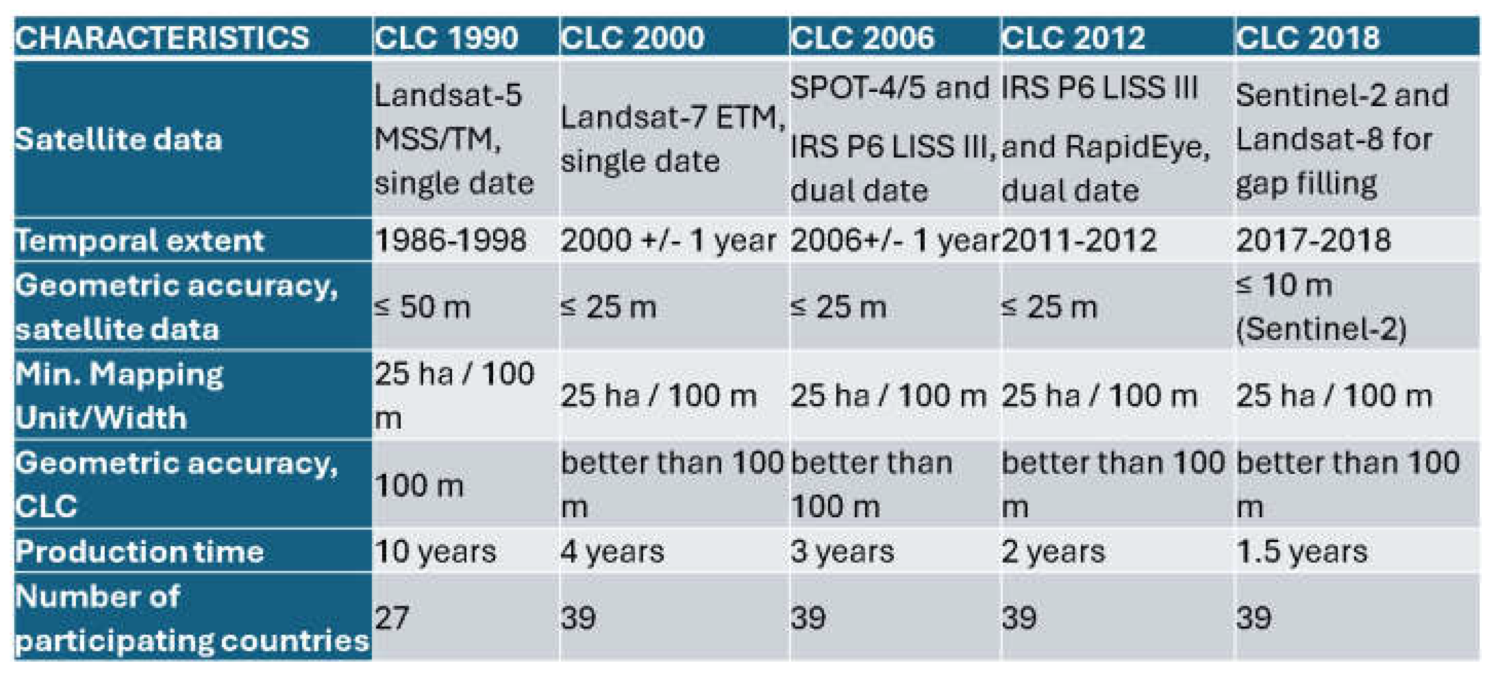
Figure 2.
Images from the categories.
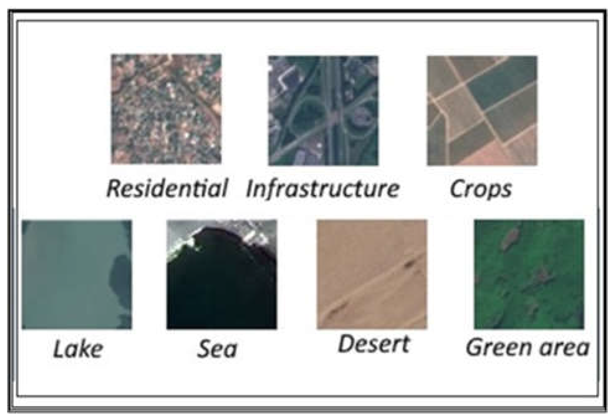
Figure 3.
The study area. In red, the boundary of the municipal territory of Reggio Calabria.
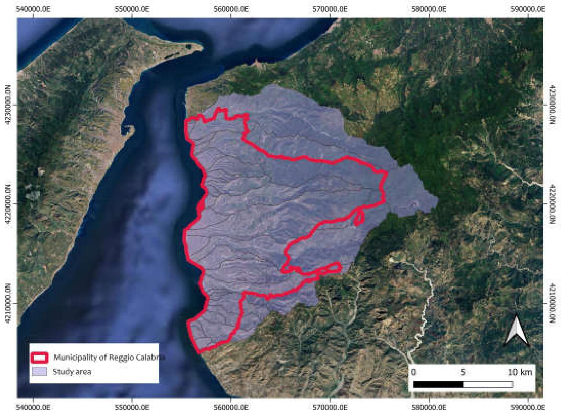
Figure 4.
A clipping of the Sentinel true-color image of the study area, acquired on 31 JMay 2024.
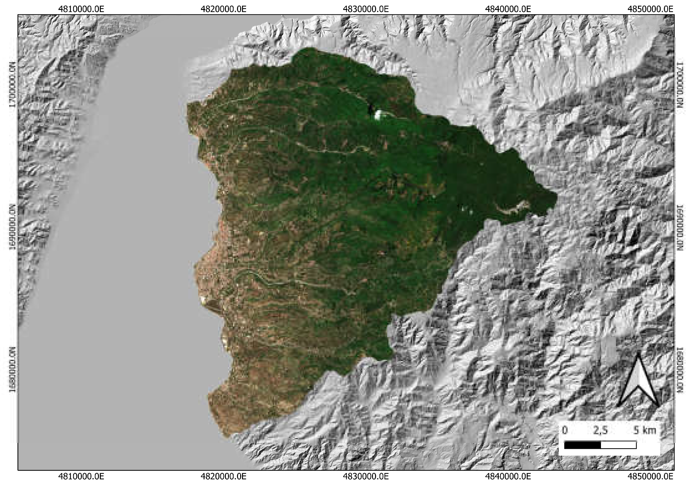
Figure 5.
Segmentation of the study area.
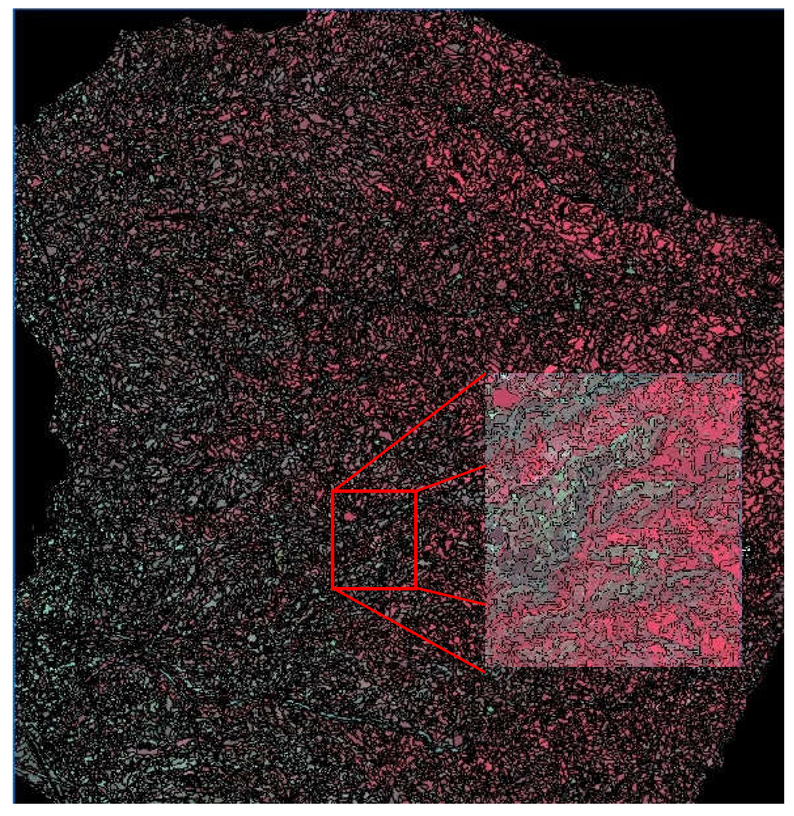
Figure 6.
Membership function defining the crisp (green) and the fuzzy (yellow) sets.
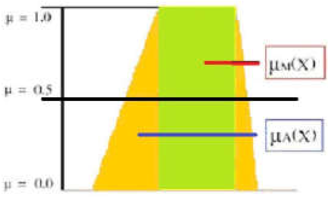
Figure 7.
Fuzzy classification of features: low, medium or high.
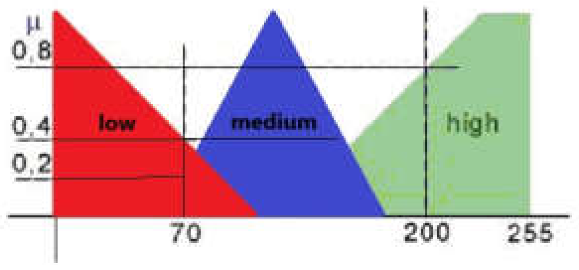
Figure 8.
Urban, water, and vegetation land cover classes.
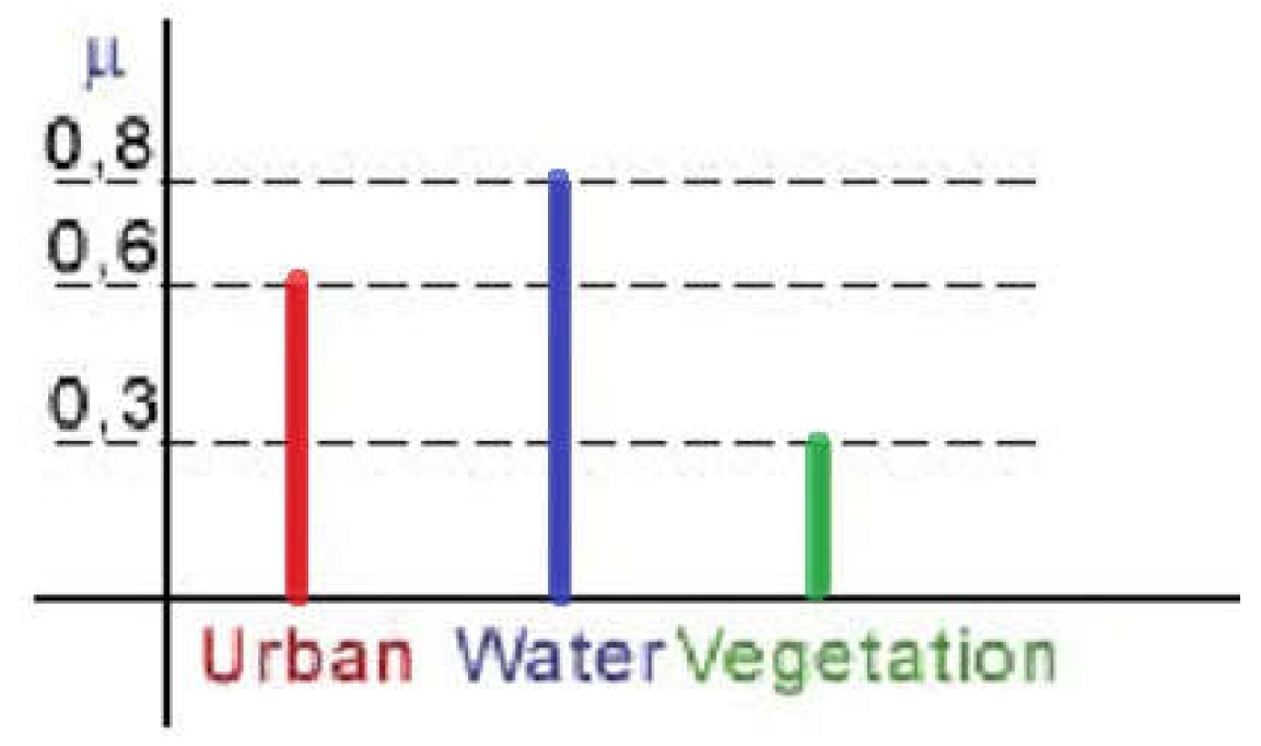
Figure 9.
Urban, water, and vegetation land cover classes, high memberships values.
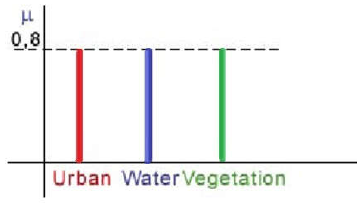
Figure 10.
Urban, water, and vegetation land cover classes, low memberships values.
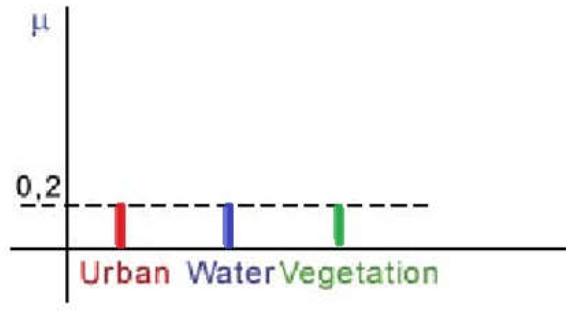
Figure 11.
Methodology steps.
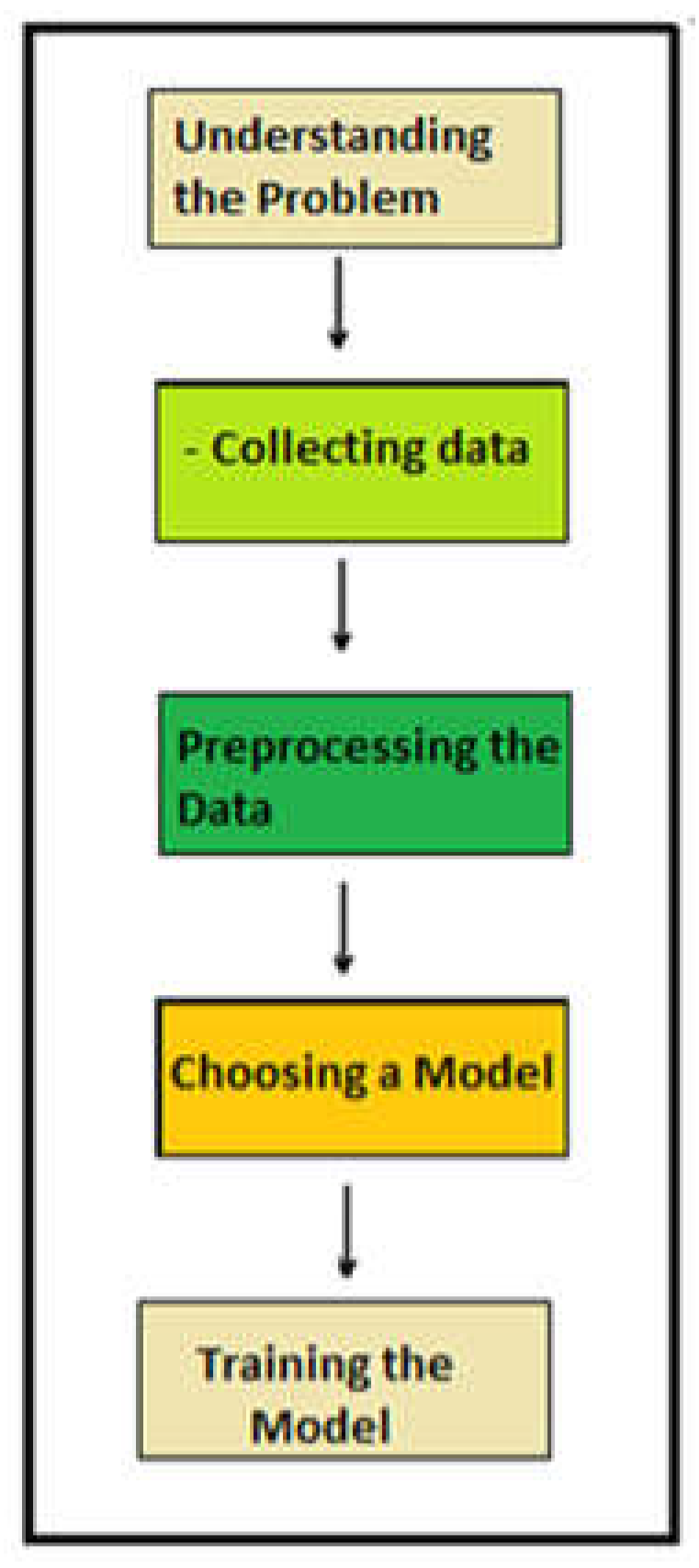
Figure 12.
Classification, derived from Sentinel-2 dataset, in eight ecotypes.
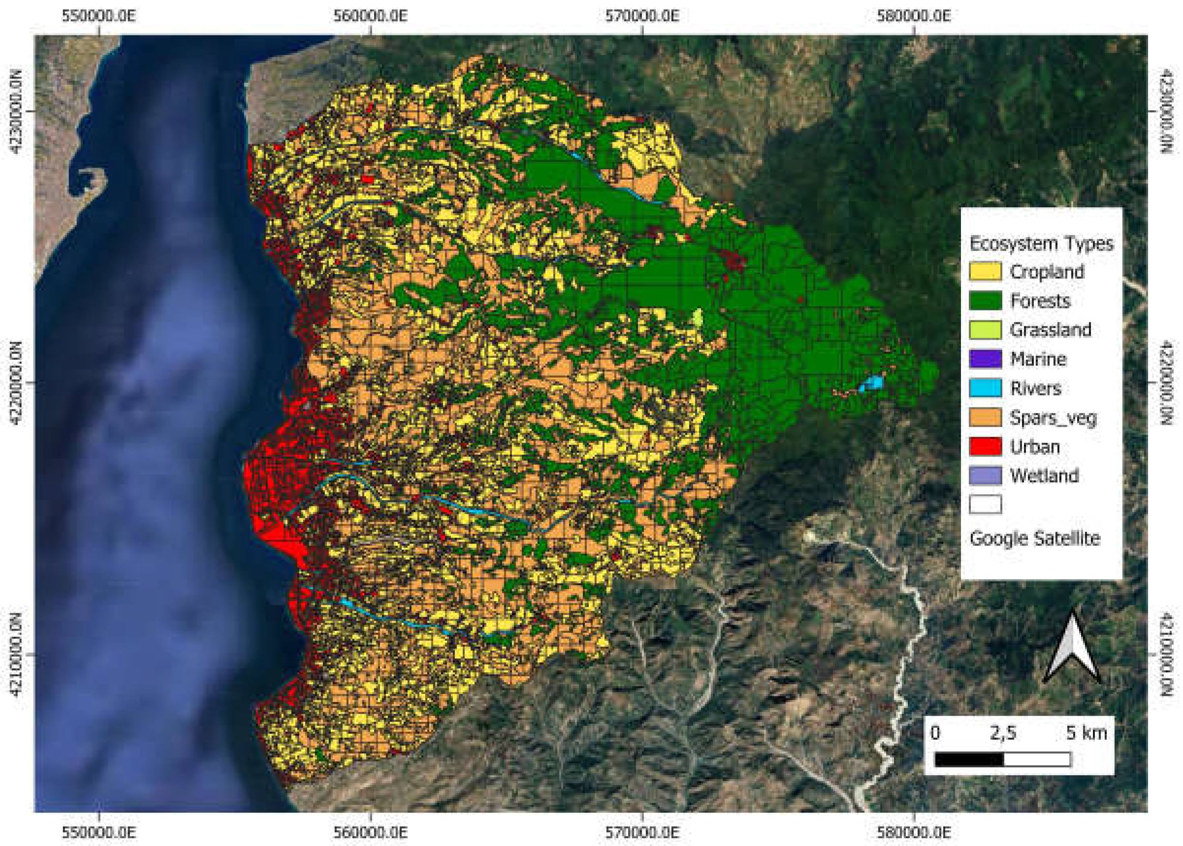
Figure 13.
ResNet: Loss diagram.
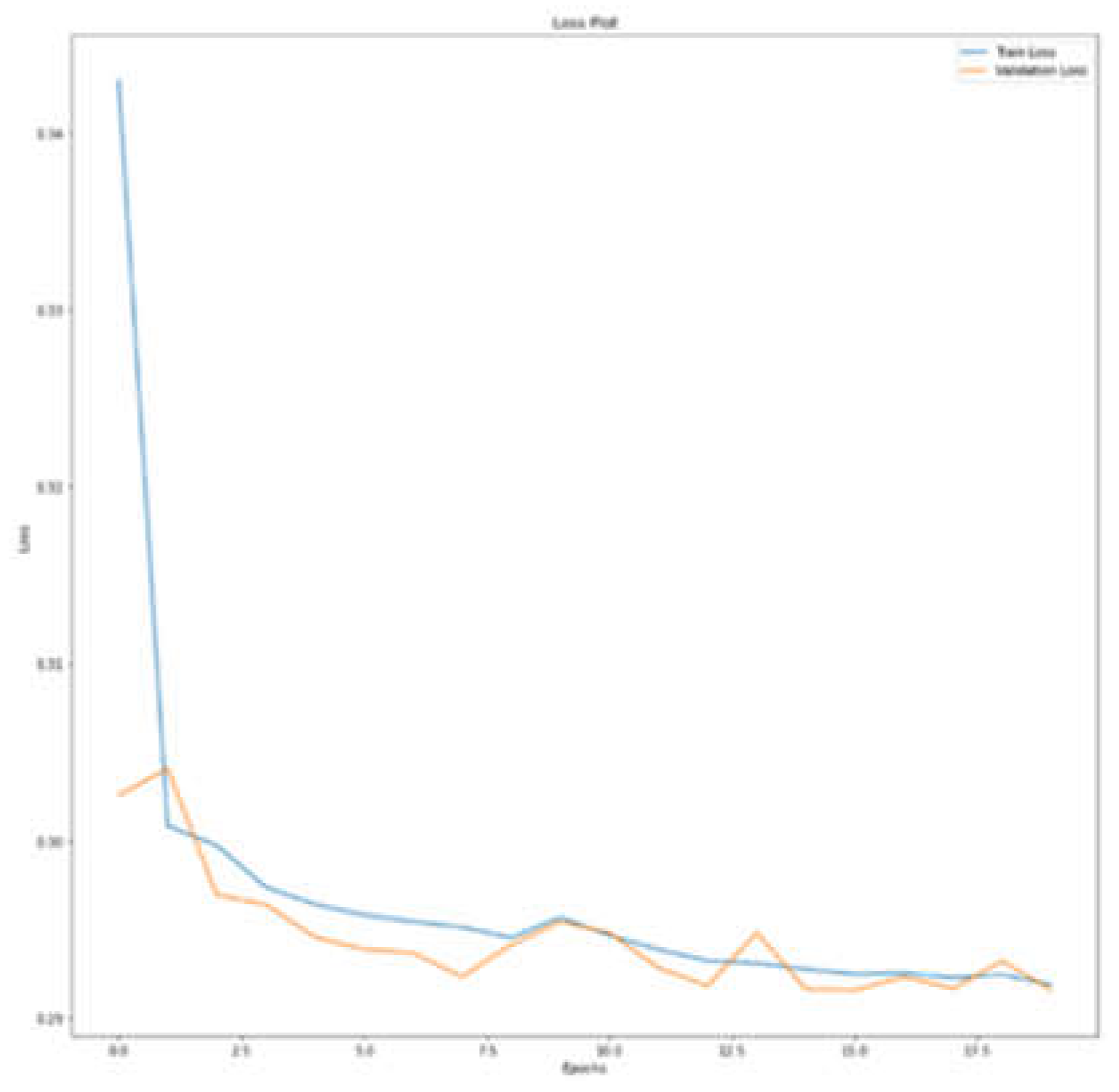
Figure 14.
ResNet: Loss diagram.
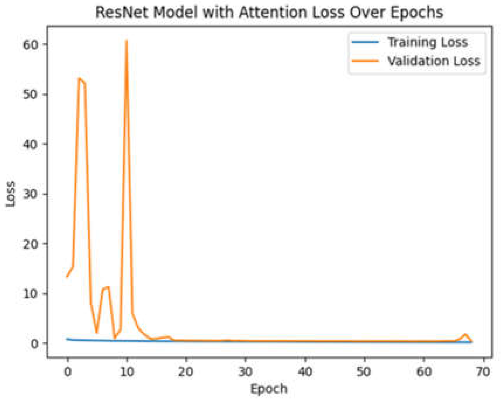
Figure 15.
ResNet: ROC/AUC curve.
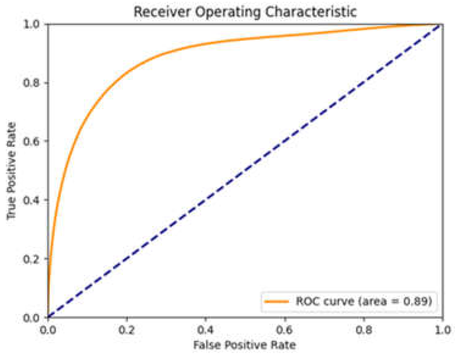
Figure 16.
ROC/AUC curve of the U-Net network.
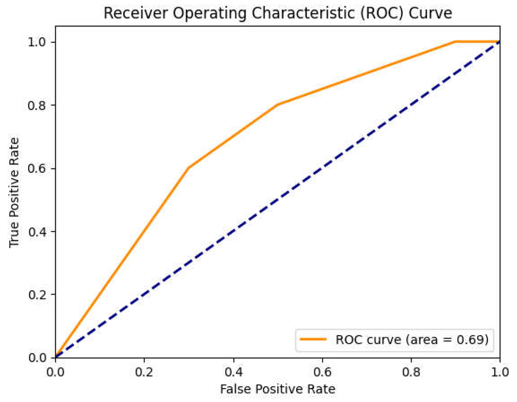

Table 1.
Parameters for multiresolution segmentation.
| Segmentation level | Bands | Scale | Homogeneity criteria | |||||||
|---|---|---|---|---|---|---|---|---|---|---|
| Color | Shape | Shape Settings | ||||||||
| PAN | RED | GREEN | BLUE | NIR | Smoothness | Compactness | ||||
| Preliminar | Yes | No | No | No | No | 4 | 0.7 | 0.3 | 0.8 | 0.2 |
| Level I | No | Yes | Yes | Yes | Yes | 4 | 0.7 | 0.3 | 0.8 | 0.2 |
| Level II | No | Yes | Yes | Yes | Yes | 10 | 0.7 | 0.3 | 0.8 | 0.2 |
| Level III | No | Yes | Yes | Yes | Yes | 1 | 0.7 | 0.3 | 0.8 | 0.2 |
| Level IV | No | Yes | Yes | Yes | Yes | 45 | 0.8 | 0.2 | 0.1 | 0.9 |
Disclaimer/Publisher’s Note: The statements, opinions and data contained in all publications are solely those of the individual author(s) and contributor(s) and not of MDPI and/or the editor(s). MDPI and/or the editor(s) disclaim responsibility for any injury to people or property resulting from any ideas, methods, instructions or products referred to in the content. |
© 2025 by the authors. Licensee MDPI, Basel, Switzerland. This article is an open access article distributed under the terms and conditions of the Creative Commons Attribution (CC BY) license (http://creativecommons.org/licenses/by/4.0/).
Copyright: This open access article is published under a Creative Commons CC BY 4.0 license, which permit the free download, distribution, and reuse, provided that the author and preprint are cited in any reuse.


