Preprint
Article

This version is not peer-reviewed.

Exploring Diverse AI Models for Enhanced Land Use and Land Cover Classification in the Nile Delta, Egypt Using Sentinel-Based Data

Submitted:

16 February 2025

Posted:

17 February 2025

You are already at the latest version

Abstract

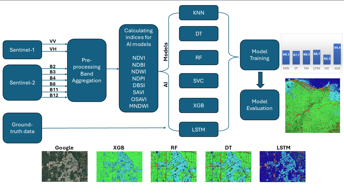
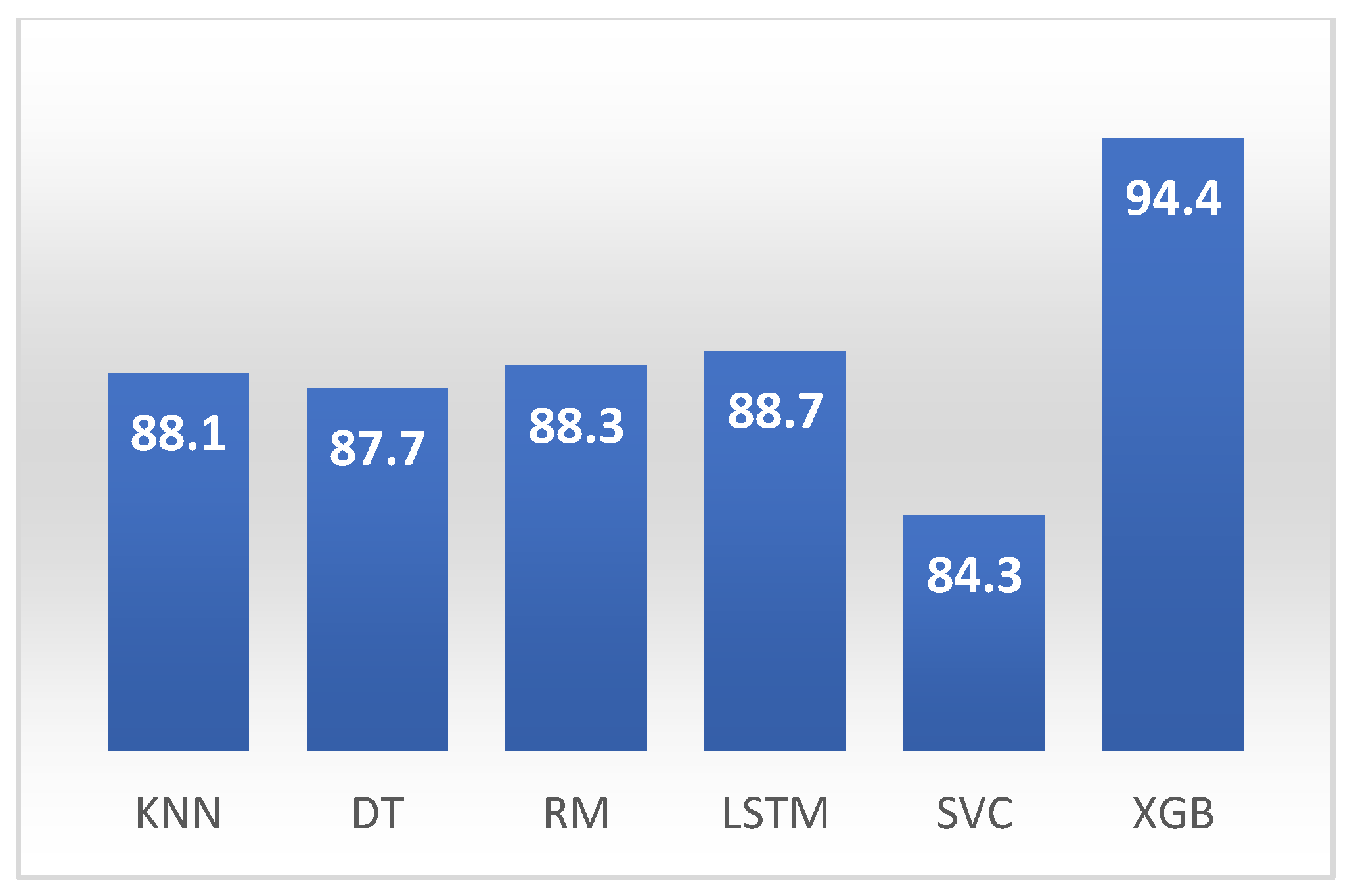
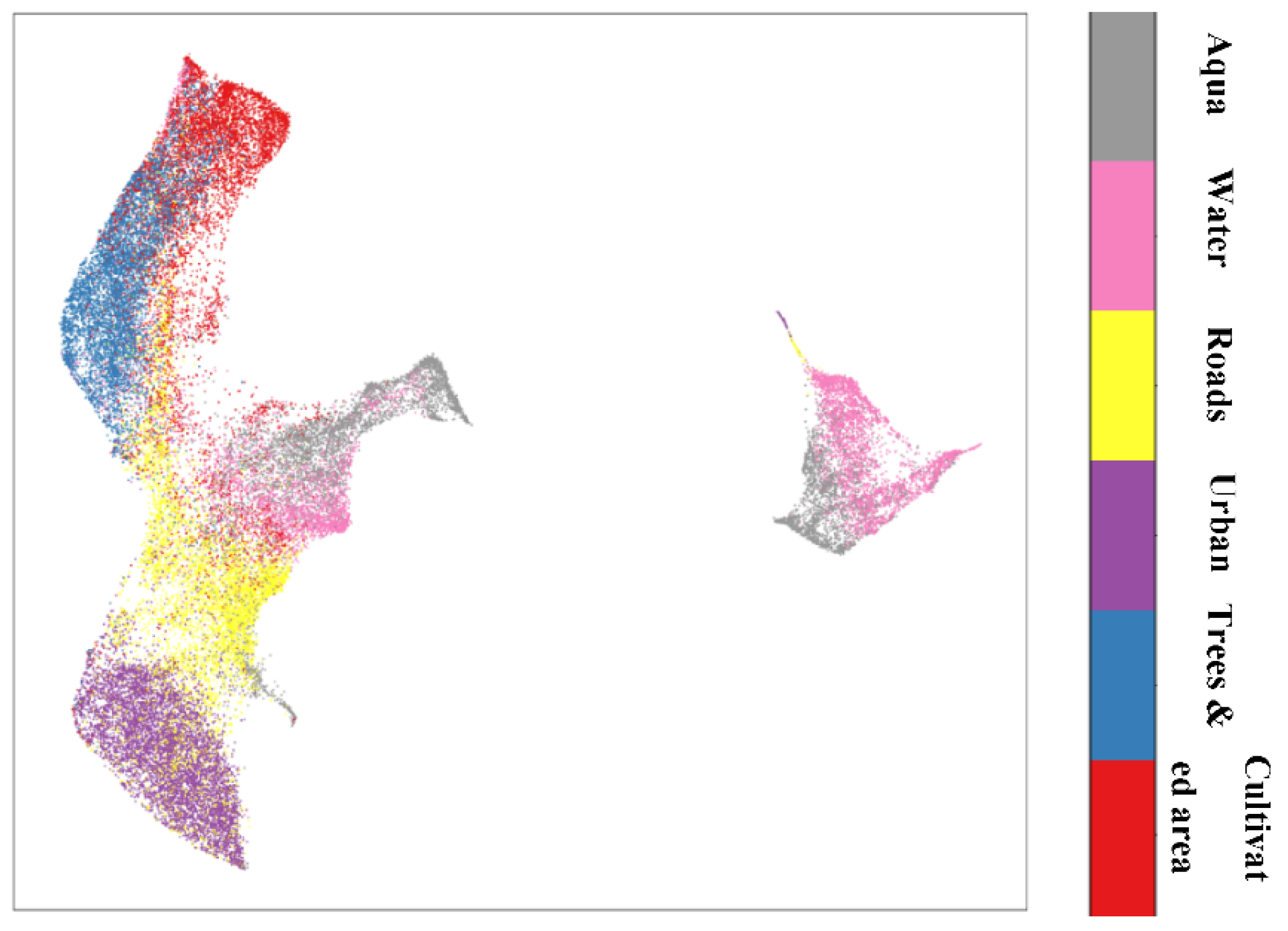
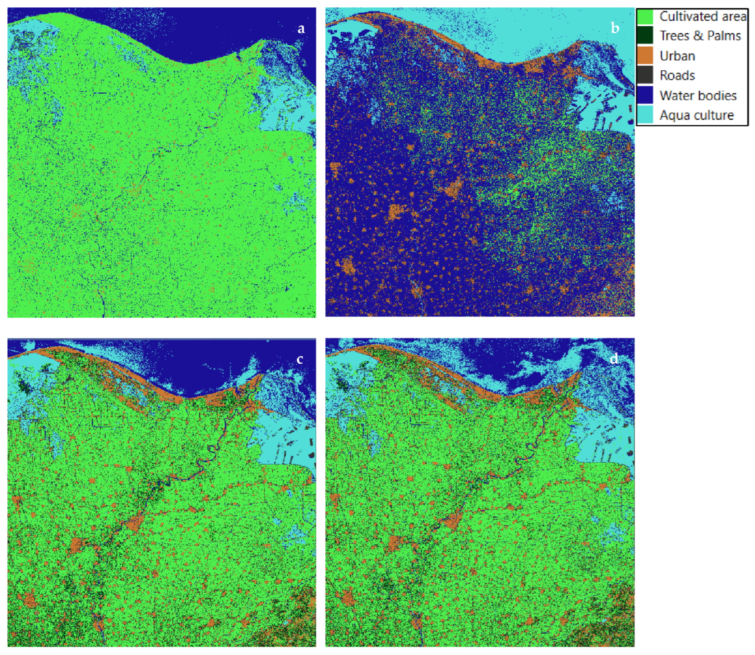
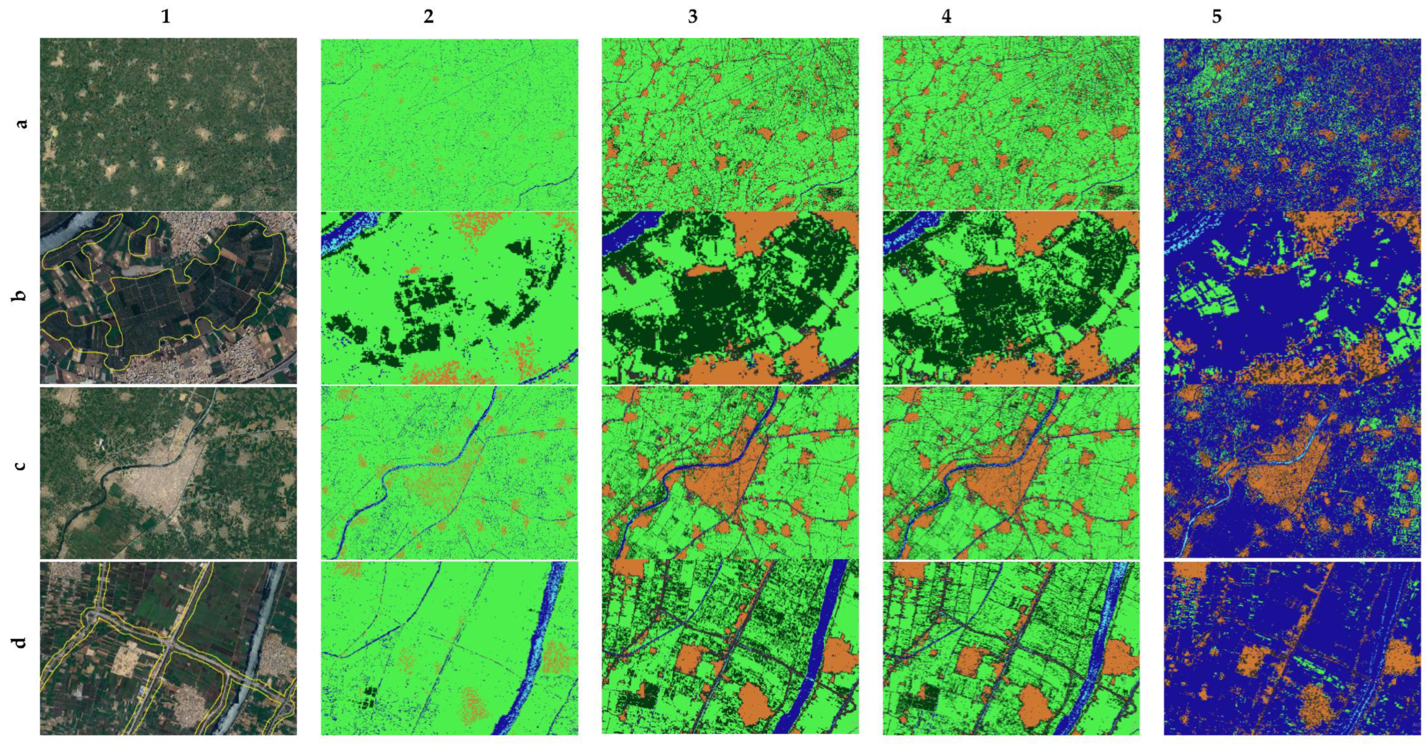
This study investigated Land Use and Land Cover (LULC) classification east of the Nile Delta, Egypt, using Sentinel-2 bands, spectral indices, and Sentinel-1 data. The aim was to enhance agricultural planning and decision-making by providing timely and accurate information, addressing limitations of manual data collection. Several Machine Learning (ML) and Deep Learning (DL) models were trained and tested using distinct temporal datasets to ensure model independence. Ground truth annotations, validated against a reference Google satellite map, supported training and evaluation. XGBoost achieved the highest overall accuracy (94.4%), surpassing the Support Vector Classifier (84.3%), while Random Forest produced the most accurate map with independent data. Combining Sentinel-1 and Sentinel-2 data improved accuracy by approximately 10%. Strong performance was observed across Recall, Precision, and F1-Score metrics, particularly for urban and aquaculture classes. Uniform Manifold Approximation and Projection (UMAP) technique effectively visualized data distribution, though complete class separation was not achieved. Despite their small size, road area predictions were reliable. This research highlights the potential of integrating multi-sensor data with advanced algorithms for improved LULC classification and emphasizes the need for enhanced ground truth data in future studies.

Keywords: 
;  ;  ;  ;  

1. Introduction

The agri-food sector is a cornerstone of Egypt’s economy, providing livelihoods for millions and significantly contributing to national food security. Despite the predominantly desert landscape, with approximately 96% of the country classified as such, agriculture flourishes in the fertile Nile Valley and Delta. This cultivated area, totaling 9.6 million acres (approximately 4% of Egypt’s landmass), supports a vital socioeconomic sector. In 2022, agriculture employed roughly 18.9% of the Egyptian workforce and contributed 11.5% to the Gross Domestic Product during the 2021/2022 fiscal year, demonstrating a 4.0% growth rate [1].
Land Use and Land Cover (LULC) change is a key indicator for understanding dynamic shifts in geographic distribution. It plays a crucial role in analyzing a range of interconnected issues, from global ecological processes and climate change to environmental security, terrestrial-marine interactions, and the maintenance of ecological balance [2,3,4,5]. LULC data play a vital role in a range of geospatial analysis tools, including urban planning, regional management, and environmental conservation efforts [6,7,8,9,10,11]. The rapid pace of urbanization has exacerbated climate change effects, underscoring the necessity for accurate land cover classifications to combat urban heat islands and monitor changes in vegetation indices, urban expansion, and aquatic structures [12].
Moreover, discussions about LULC offer vital frameworks for understanding the intricate relationships between human societies and our planet’s ecosystems. By conducting thorough LULC analyses, researchers obtain critical insights into socio-ecological dynamics, which are fundamental for promoting sustainable resource management, agricultural planning, and food security initiatives [11,13,14]. Up-to-date and accurate LULC maps are crucial for enhancing sustainable resource management, shaping agricultural and environmental policies, and assessing the ecological impacts of economic and agricultural activities [6,15,16,17,18,19,20,21]. Food security relies heavily on accurate information about agricultural land. This information is necessary for environmental monitoring, effective crop management, and meeting national crop demands. Deep Learning (DL) provides innovative tools for acquiring this crucial data [22].
Despite progress, challenges remain in the precise mapping of LULC, primarily due to insufficient up-to-date reference data and the labor-intensive nature of traditional surveying techniques [23]. Innovations in satellite technology and computing have not only increased access to open-source satellite data but also enhanced the capabilities of Remote Sensing (RS) for LULC mapping [24]. These advancements allow for the detailed detection, identification, and tracking of LULC changes across a range of spatial and temporal dimensions [25]. However, ground-level validation, potentially using geotagged photos, is crucial for verifying the accuracy of LULC maps [26,27].
RS cartography has been transformed by the rapid development of Earth observation systems, enabling its application across a wide spectrum of fields, from monitoring urban growth and responding to disasters to classifying vegetation, assessing forest degradation and wildfire damage, and studying climate change [28,29,30,31,32,33,34]. The popularity of RS technology stems from its ability to provide thorough information quickly and efficiently [35,36]. However, the reliance on commercial satellite data presents a significant hurdle. The cost of such data can be prohibitive, and coverage may be limited, particularly in certain regions. This underscores the critical need for advancements in multi-source and multi-temporal remote sensing techniques [37,38]. The emergence of free and open data sources, such as the Sentinel-2 (optical) and Sentinel-1 (SAR) missions since 2015, represents a major step forward, democratizing access to valuable Earth observation data and fostering innovation in RS applications [37,39,40].
Analyzing LULC using RS data often presents a significant challenge due to the sheer volume of data, making manual analysis labor-intensive, time-consuming, and expensive [41]. Artificial Intelligence (AI) has emerged as a transformative technology in this domain, offering the potential to automate image interpretation and efficiently extract valuable spatial information from satellite imagery [42,43]. Established Machine Learning (ML) algorithms, such as K-Nearest Neighbors (KNN) and Random Forest (RF), have proven useful in a variety of applications, from recognizing patterns in forests to performing land classification, regression, and clustering [44,45,46,47,48]. However, DL techniques, with their ability to handle both pixel-based and object-based classification, are particularly well-suited for the task of deciphering the complex and nuanced patterns that characterize remote sensing imagery. The development and refinement of these AI-driven approaches are crucial for unlocking the full potential of remote sensing data in LULC analysis [41,49,50].
Several ML algorithms gained prominence in RS for LULC classification during the 1990s, including Support Vector Machines (SVM), Decision Trees (DT), and RF. Their adoption was further accelerated by advancements in computer chip multithreading in the 2000s [46,47,51,52,53,54,55]. More recently, Extreme Gradient Boosting (XGBoost) has emerged as a powerful technique, leveraging an innovative approach to gradient-boosted DT [56,57]. Artificial Neural Networks (ANNs) have also seen significant progress, although their effectiveness depends on prior knowledge derived from ground samples and the quality of training data [56,58]. A common challenge for these methods is the presence of mixed pixels, which can negatively impact classification accuracy [59]. To address the temporal dimension of image data, Recurrent Neural Networks (RNNs), particularly Long Short-Term Memory (LSTM) models, have been employed for classifying image time series, capitalizing on their ability to learn sequential relationships [60,61,62,63,64].
For effective crop management and environmental conservation, automated information classification is increasingly vital. A key challenge lies in the variability of ground object characteristics and imaging conditions, which can negatively influence classification accuracy [65,66]. While spectral bands are important, the analysis of RS images also relies heavily on Vegetation Indices (VIs) and texture features. However, the computational cost associated with processing such high-dimensional data can be a limiting factor for many ML techniques [67].
In the current study, we leverage Sentinel-2 and Sentinel-1 data, alongside ML and DL algorithms, to classify LULC patterns in the east of Delta, Egypt, to overcome the current obstacles to accurately identify agricultural lands and crops areas. By incorporating ground annotations and labelled images from Google Earth, we evaluate the performance of various ML and DL models across different scenarios and dates in July and August 2021. Our comprehensive analysis suite aims to enhance our understanding of feature importance at the individual LULC class level, utilizing Python programming for interpretation.

2. Materials and Methods
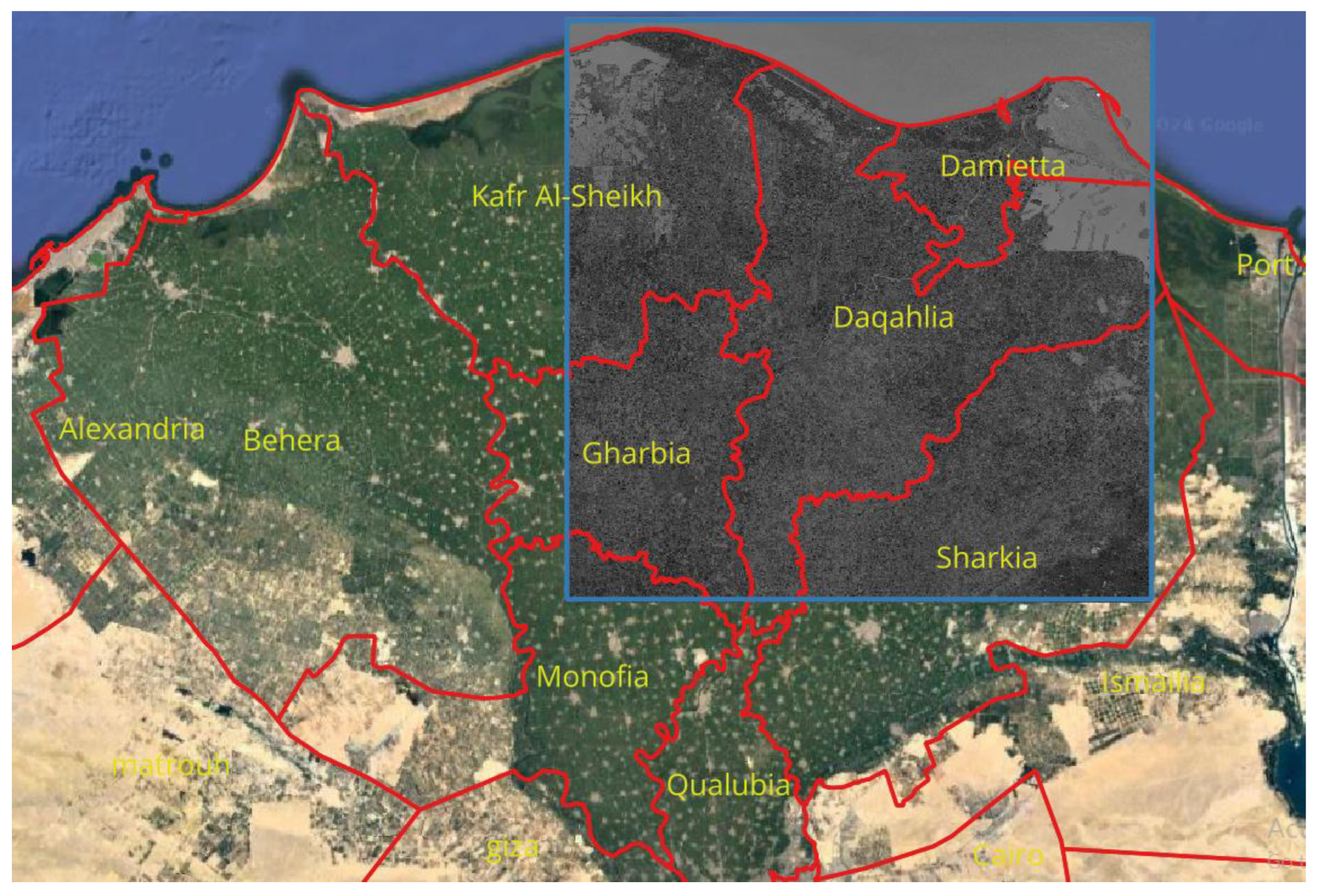
2.1. Case Study

This study aimed to evaluate a developed classification method in the eastern region of the Nile Delta in Egypt (Figure 1). Located in northern Egypt where the Nile River converges with the Mediterranean Sea, the Nile Delta extends approximately 150 km north from Cairo. This region is crucial, as it is home to over 50% of Egypt’s population and supports 63% of the nation’s agricultural land. The delta features sandy and silty coastlines with various lateral configurations, shaped by the historical paths of the Nile [68]. The study area includes governorates such as Daqahlia, Damietta, Sharkia, Gharbiya, and Kafr Al-Sheikh, covering about half of the delta, with a total area of approximately 10,610.88 kmÂČ. Known for its fertile soil rich in clay, this region is marked by small-scale agricultural fields and densely populated settlements engaged in diverse agricultural activities, including crop cultivation and livestock farming. The Nile Delta’s fertile soil and favorable climate create ideal conditions for intensive agriculture, significantly contributing to Egypt’s agricultural output. Its strategic location along the Mediterranean coast and its proximity to the Nile River enhance irrigation and support year-round agricultural practices.

2.2. Data Annotation

Ground-truth reference samples were manually labeled using geo-tagged shapefiles obtained from Google Earth and processed with QGIS software (open-source) version 3.32-Lima (Creative Commons Attribution-ShareAlike 3.0 license (CC BY-SA), https://qgis.org/de/site/). The annotated shapefile included six classes: cultivated areas, forests (including trees and palms), urban, roads, water bodies, and aquacultures, totalling 11,637 polygons. This reference geo-tagged shapefile was utilized to calibrate the classifiers and assess the classification accuracy.

2.3. Satellite Image Processing

2.3.1. Sentinel-1 Data

The Sentinel-1 satellite features a C-band Synthetic Aperture Radar (SAR) instrument that operates at a central frequency of 5.405 GHz. Sentinel-1 data is available in the Ground Range Detected (GRD) format. Accessing this data was done via the ’Earth Engine Data Catalog,’ utilizing Python 3 with the command ’ee.ImageCollection(“COPERNICUS/S_GRD”).’ The preprocessing of Sentinel-1 data was performed using the Sentinel-1 Toolbox. This preprocessing process involved eliminating thermal noise, radiometric calibration, and terrain correction. The data were gathered in Interferometric Wide Swath (IW) mode, with a coverage width of 250 km. Sentinel-1 data were captured using dual polarizations, VV and VH, during the descending orbital trajectory. The pixel size and resolution of the data are 10 meters [69].
To ensure alignment with the Area Of Interest (AOI), the Sentinel-1 data were processed to have the same geometry coordinates as the downloaded Sentinel-2 tile. In cases where the AOI spanned across multiple Sentinel-1 tiles, a merging function was applied using the ’rasterio’ library in Python. Given that Sentinel-1 data were obtained from different orbits, the Coordinate Reference System (CRS) was corrected to match that of Sentinel-2 (EPS: 32636), ensuring consistency in geospatial referencing.

2.3.2. Sentinel-2 Data

Data from Sentinel-2 were accessed through the Microsoft Planetary Computer, employing Python 3 with the command ’Planetary_computer.’ This platform is an open-source resource that follows open standards. The Sentinel-2 imagery consists of thirteen spectral bands with resolutions ranging from 10m to 60m and has a revisit period of about five days. The data were processed to Level-2A (bottom-of-atmosphere) using Sen2Cor and then the data was transformed to a cloud-optimized GeoTIFF format. Terrain correction was carried out using the Planet DEM 30 digital elevation model [70]. To ensure consistency with the resolution of Sentinel-1 data, the Sentinel-2 bands with a spatial resolution of 20m were resampled to 10m using nearest neighbour interpolation.
The AOI was covered by a single tile with the ID ’36RUV’. The downloaded data had a cloud cover of equal to or less than 4%. The downloaded bands included red, green, blue, near-infrared (NIR), red-edge-1, SWIR-1, and SWIR-2. The CRS used was ’EPS: 32636’ for consistent geospatial referencing.

2.4. Additional Features for Sentinel-1 and 2 Bands

Additional features were derived from Sentinel-1 and Sentinel-2 bands to enhance LULC classifications. The ratio between VV and VH polarizations was computed from Sentinel-1 data. Furthermore, various spectral indices were calculated from Sentinel-2 bands to aid in the identification of LULC classifications. The utilized spectral indices from Sentinel-2 bands are detailed in Table 1.
For the training and prediction of the models, data were gathered from nine selected dates in July and August 2021 for both Sentinel-1 and Sentinel-2. These dates were specifically chosen to ensure they were closely aligned, with a difference ranging from 1 to 3 days, as illustrated in Table 2. Moreover, one date from 2023 was designated for testing the models using the latest imagery from Google Earth. The Sentinel-2 image dated August 6, 2023, underwent adjustments to reflect the shift in the baseline of the Sentinel orbit from 3.0 to 4.0, which commenced on January 25, 2022 [71,72].

2.5. Data Preprocessing

The satellite imagery from Sentinel-1 and Sentinel-2 was combined with the annotated shapefile to enable pixel-level annotation. Each pixel’s information consisted of values from the spectral bands and indices used as features, along with the corresponding LULC class from the annotated shapefile, which acted as the label. This annotation process covered nine dates throughout the summer of 2021. However, the dataset exhibited imbalanced class distributions due to the uneven spatial distribution of ground objects, particularly with aquaculture being more prevalent in the northern regions of the Nile Delta and the Mediterranean coast. This imbalance could adversely affect the accuracy of ML classifications [73]. To address this challenge, techniques for managing imbalanced classes, including the decomposition-based method and the Synthetic Minority Over-sampling TEchnique (SMOTE), were applied [74]. Additionally, the dataset was normalized and divided into training and testing sets in an 80-20% ratio. These steps were crucial for improving the accuracy of ML classification efforts, as emphasized by Buda et al. [73].

2.6. AI Models

For classifying the evolved dataset of Sentinel-1, Sentinel-2, and the annotated shapefile, five machine learning classification models and one DL model were developed. The utilized machine learning algorithms include KNN, Support Vector Classifier (SVC), DT, RF, and XGB. Additionally, a LSTM model was employed as the deep learning approach. To enhance performance, the XGB and SVM classifiers were configured to run on the GPU instead of the CPU. For XGB, the device parameter was set to ’cuda’, and the thundersvm library was used in place of sklearn, with the gpu_id parameter adjusted to the GPU ID number. Furthermore, various parameters were tuned for each classifier using the RandomizedSearchCV library to optimize performance and achieve higher accuracy. Details of the optimization process can be found in Table 3.
Table 1. Utilized spectral indices from Sentinel-2 bands.
Spectral index Formula Characteristics / Definitions References
Normalized difference vegetation index (NDVI) NDVI= (NIR – R)/(NIR+R) Measures vegetation health by comparing the reflectance of near-infrared (NIR) and red light, with NIR being reflected by vegetation and red light being absorbed by vegetation. [75]
kernel Normalized difference vegetation index (kNDVI) kNDVI = tanh((NIR – red/ 2σ)2)σ = 0.5 (NIR + red) Enhances the performance of NDVI by incorporating automatic and pixel-wise adaptive stretching, ensuring that all aspects of the relationship between NIR and red bands are considered. [76]
Normal Difference Built-up Index (NDBI) NDBI = (SWIR – NIR) / (SWIR + NIR) Asserts built-up areas by utilizing the NIR and short-wave infrared (SWIR) bands. [77]
Dry Bare Soil Index (DBSI) DBSI = ((SWIR – GREEN) / (SWIR + GREEN) ) – NDVI Combines spectral bands including blue, red, NIR, and SWIR to capture variations in soil composition. [78]
Normal Difference Water Index (NDWI) NDWI = (GREEN - NIR) / (GREEN + NIR) Identifies open water features in satellite imagery, distinguishing water bodies from soil and vegetation. [79]
Modified Normalized Difference Water Index (MNDWI) MNDWI = (GREEN − SWIR1)/(GREEN + SWIR1) Effectively distinguishes between water bodies and urban areas in satellite images. [80]
Normalized Difference Pond Index (NDPI) NDPI = (SWIR1 - GREEN)/(SWIR1 + GREEN) Exhibits enhanced discriminatory power for aquatic and wetland vegetation compared to NDVI, which is a general indicator of vegetation presence. [81]
Shortwave infrared transformed reflectance (STR) STR = (1 - SWIR)2 / 2 SWIR Calculates reflectance for bare soils using SWIR bands. [82]
Soil adjusted vegetation index (SAVI) SAVI= 1.5(NIR – R) (NIR+R+0.5) Reduces the influence of soil brightness by incorporating a correction factor for soil-brightness. [83]
Optimized soil adjusted vegetation index (OSAVI) OSAVI= 1.16(NIR – R)/ (NIR+R+0.16) A modified version of SAVI that utilizes reflectance in the red and NIR spectrum. [84]
Enhanced vegetation index (EVI) EVI= 2.5(NIR – R)/(NIR+6 R – 7.5B+1) Similar to NDVI, but EVI incorporates corrections for atmospheric influences and canopy background effects, thereby enhancing its sensitivity, notably in densely vegetated regions. [85]
Automated Water Extraction Index (AWEI) AWEIsh = BLUE + 2.5 × GREEN − 1.5 × (NIR + SWIR1) − 0.25 × SWIR2 Contributes to enhanced land cover classification accuracy through its capacity to discriminate between binary water and non-water areas irrespective of environmental conditions. [80]
The LSTM model architecture comprises six ’Bidirectional’ LSTM layers with neuron numbers set to 16, 32, 64, 64, 32, and 16, respectively, with an input shape of (20, 1) corresponding to the number of features. Dropout layers were included after each LSTM layer, with a dropout rate of 20%. The final layer consists of six neurons representing the six classes, with the activation method set to softmax. The model was compiled with ’sparse_categorical_crossentropy’ loss, ’adam’ optimizer, and accuracy as the displayed metric. The total number of parameters in the model was 235,590. Training was conducted for 100 epochs with a batch size of 8192, and a validation split of 0.1 was used.
Table 2. Dates of imagery utilized in the study.
Sentinel-1 Sentinel-2
July 04, 2021 July 07, 2021
July 10, 2021 July 12, 2021
July 16, 2021 July 17, 2021
July 28, 2021 July 27, 2021
August 03, 2021 August 01, 2021
August 09, 2021 August 11, 2021
August 15, 2021 August 16, 2021
August 21, 2021 August 21, 2021
August 27, 2021 August 26, 2021
August 07, 2023 August 06, 2023
Table 3. Range of Parameters Used by RandomizedSearchCV for Each ML Model.
Model Search space
KNN n_neighbors = [4, 5, 6, 7, 8, 9]
DT Criterion = {‘gini’, ‘entropy’}, max_depth = [10,13,15,18,20], min_sample_split = [50,80,100]
RF n_estimators = [500,700,1000], max_depth = [10,13,15,18,20], min_sample_split = [50,80,100]
SVC Kernels = ’RBF’, C = [10,20,30,40], Gamma = [0.1,0.5,1,5,10]
XGB n_estimators = [500,700,1000], max_depth = [5,8,10,12,15], gamma = [0,0.001,0.005,0.1,0.5], learning_rate = [0.1,0.5,0.8,1,1.2,1.5,2], tree_method = ‘hist’

2.7. Models’ Evaluation

To assess the performance of the utilized models with the best parameters, various metrics were calculated, including accuracy, recall, precision, and F1 score. These metrics are computed using the following equations:
A c c u r a c y =   T P + T N T P + F P + T N + F N
P r e c i s i o n = T P T P + F P
R e c a l l = T P T P + F N
F 1   s c o r e = 2 × P r e c i s i o n × R e c a l l P r e c i s i o n + R e c a l l
Where TP (True Positive), TN (True Negative), FP (False Positive), and FN (False Negative) denote the predicted classifications.

2.7. Experiment and Analysis

The verification and simulation of the proposed method were conducted on a high-performance laptop, ensuring consistency across all comparison methods in a unified software and hardware environment. The experimental hardware and software configurations are detailed in Table 4. All experimental codes for remote sensing and AI models proposed in this paper were implemented using the Python programming language.

3. Results

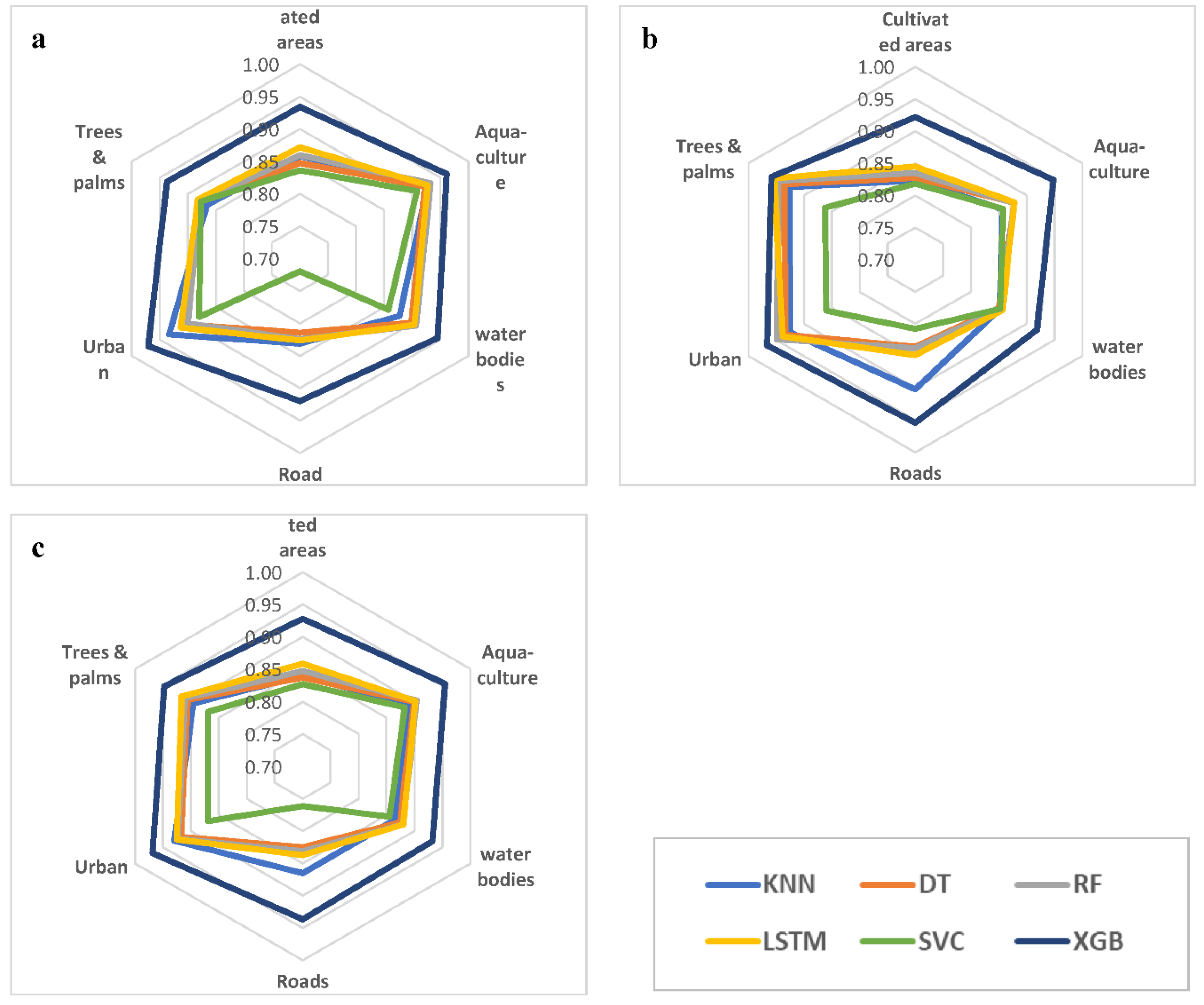
3.1. Models’ Performance

The analysis of various machine learning models in Figure 2 revealed a notable Overall Accuracy (OA) across all tested scenarios, with the best-performing scenario achieving a mean OA of 91.05 ± 3.35%. Among the models evaluated, the XGB model stood out, achieving the highest accuracy at 94.4%. This marked a significant improvement over the other models, highlighting XGB’s superior classification capability. In contrast, the SVC model exhibited the lowest OA at 84.3%, closely aligned with several of its peers, indicating a more consistent but less effective performance.
The models, including DT, KNN, RF, and LSTM, demonstrated comparable accuracies, with values recorded at 87.7%, 88.1%, 88.3%, and 88.7%, respectively. Interestingly, the SVC model displayed a general decline in accuracy as the number of variables increased. This decline was contingent upon the nature of the variables included, suggesting that the model’s sensitivity to input features played a critical role in its performance.
For the LSTM model, an important observation was made: its accuracy reached 88% after 40 epochs of training, stabilizing at 88.7% from epoch 80 onward. Validation accuracy also exhibited a trend of being consistently higher than overall accuracy, particularly converging around epoch 84, as illustrated in Figure 3. This stability suggests that the LSTM model effectively captured the underlying patterns in the data, although it took time to reach optimal performance.
The performance metrics for individual classes, as showcased in a radar chart in Figure 4, revealed a consistent pattern across the best-performing models. The XGB model excelled in precision, recall, and F1-Score metrics, with all exceeding 92%. Specifically, the Urban and Aqua-culture classes achieved impressive precision and recall rates, reaching 97% and 96%, respectively. In contrast, the Roads class consistently exhibited lower performance, with precision, recall, and F1-Score values ranging from 82% to 85% across most models. The KNN model showed a noteworthy exception, achieving 90% precision and 87% F1-Score, indicating its relative effectiveness in this particular classification task.
The SVC model struggled the most with the Roads class, recording the lowest metrics: recall at 72%, precision at 81%, and F1-Score at 76%. Conversely, the XGB model demonstrated significant strength in classifying Roads, achieving recall, precision, and F1-Score values of 92%, 95%, and 94%, respectively. The Cultivated Areas class also demonstrated lower performance across the board, with metrics ranging from 82% to 87% for most models, while XGB improved these values to between 92% and 94%.
For the Trees and Palms class, precision metrics were consistently high across all models, ranging from 93% to 96%. The only outlier was the SVC, which recorded a lower precision of 86%. Notably, the XGB model achieved significantly higher recall for this class at 94%, surpassing the 87% to 88% recall rates of the other models, demonstrating its ability to identify relevant features effectively. This trend was mirrored in the F1-Score, which exhibited similar patterns to recall with slightly higher values.
The Water Bodies class presented an interesting case; the XGB model recorded a precision of 92%, while other models fell in the range of 85% to 86%. However, recall for Water Bodies was relatively high across all models, with the XGB model achieving 95% and the others ranging from 86% to 91%. This suggests that while XGB led in precision, all models performed adequately in identifying Water Bodies.

3.2. Data Visualisation

To visualize the distribution and separability of input features for the 2021 dataset, we employed Uniform Manifold Approximation and Projection (UMAP). This technique is valuable for dimensionality reduction and visualization, as it preserves local structures and relationships among data points. In the UMAP plot shown in Figure 5, each color represents a distinct class among the six classes. Effective classification is indicated by closely clustered points of the same color and increased separation between different colors. The resulting UMAP visualizations illustrated clear separations among certain classes—specifically, the Cultivated Areas and Trees & Palms, Water Bodies and Aqua-culture—while the Roads class showed some overlap with other classes.

3.2. Models’ Evaluation

The application of the established models to the entire satellite image tile covering the AOI provided insightful results. These results were visualized as geo-images, maintaining the same spatial coordinates as the original satellite imagery, as shown in Figure 6. Conducted on June 8, 2023, this comprehensive analysis focused on the detailed results from the XGB, RF, DT, and LSTM models. The SVC and KNN models were excluded from this detailed evaluation due to their lower OA, precision, and F1-Score, as well as their significantly longer computation times, which extended from 12 to 18 weeks.
The resulting distribution maps vividly illustrated the prevalence of various LULC classes, with the XGB model indicating Cultivated Areas as the dominant class. In contrast, the LSTM model identified Water Bodies as predominant. The RF and DT models produced similar results, primarily highlighting the dominance of Cultivated Areas while providing clearer representations of the other classes.
For a more granular examination of LULC class distribution, Figure 7 presents a zoomed-in view of a specific area within the AOI. This detailed comparison juxtaposes model predictions against Google satellite imagery for reference. The XGB model exhibited a strong representation of Cultivated Areas, correlating closely with the reference imagery. RF and DT models also accurately represented these areas, while the LSTM model incorrectly classified some low-density cultivated areas as urban.
The RF model demonstrated the most accurate depiction of Trees and Palms when compared to the Google satellite imagery, closely followed by DT. In contrast, the XGB model showed fewer areas classified as Trees and Palms, and the LSTM model misrepresented these areas as Water Bodies. For the Urban class, RF, DT, and LSTM models showed similar representations, with RF providing the most accurate portrayal relative to the Google imagery. The XGB model, however, only captured buildings as urban, misclassifying adjacent uncultivated areas.
All models successfully represented the Roads class, with RF and DT achieving the best performance. The XGB and LSTM models depicted roads with thinner lines compared to the reference imagery. Significantly, the XGB model excelled in predicting Water Bodies, distinguishing this class from aqua-culture more effectively than RF and DT, which sometimes conflated the two. In addition, the representation of the River Nile and canals was accurate across all models, with RF demonstrating slightly better performance. Conversely, Aqua-culture areas were accurately plotted by all models, yielding similar results in their predictions.

4. Discussion

LULC classification has greatly benefited from the rapid evolution of RS technologies and the expanding availability of diverse geospatial data. The wealth of spectral and spatial information provided by multi-scale, multi-resolution sensors and thematic mappers is essential for applications ranging from regional planning and urban management to environmental monitoring [86,87,88,89]. A variety of algorithms are employed to classify this data and extract the necessary information for these applications [28].
The use of satellite images from the Sentinel-2 platform enables the calculation of diverse spectral indices, which are crucial for distinguishing features that aid in land cover mapping. The indices listed in Table 1 facilitate the differentiation of water bodies from soil and vegetation through the Normalized Difference Water Index (NDWI) [79]. They also help recognize urban areas from water surfaces using the Modified Normalized Difference Water Index (MNDWI) [80] and the Automated Water Extraction Index (AWEI) [80]. To characterize bare soil, the Shortwave Infrared Transformed Reflectance (STR) index was employed [82], while the Soil Adjusted Vegetation Index (SAVI) [83] and the Optimized Soil Adjusted Vegetation Index (OSAVI) [84] were used to mitigate soil brightness. Moreover, vegetation areas were identified using the Normalized Difference Vegetation Index (NDVI) [75] and the Kernel Normalized Difference Vegetation Index (kNDVI) [76], while built-up areas were detected through the Normalized Difference Built-up Index (NDBI) [77].
Sentinel-2 data and derived indices have been widely and successfully applied to LULC mapping, yielding consistently good accuracy [90,91]. The use of Sentinel-2 time series data has proven effective in mitigating misclassifications related to specific agricultural practices and improving the delineation of small land cover features, such as minor crop fields, rivers, and roads. Moreover, the integration of Sentinel-1 radar data with Sentinel-2 optical imagery has further boosted LULC classification accuracy. In the present study, this combined approach resulted in an approximate 10% improvement in overall accuracy, demonstrating the value of incorporating radar data. Sentinel-1’s sensitivity to surface characteristics like texture, elevation, internal structure, roughness, and moisture content [92,93,94,95] proved particularly useful in distinguishing forested areas from agricultural land [96]. However, the use of Sentinel-1 data alone has been shown to have limited effectiveness for LULC mapping [95,97,98].
Among the models used in this study, most achieved OA of approximately 88%, as illustrated in Figure 2, with the XGB model attaining the highest accuracy at 94.4%, while the SVC model recorded the lowest at 84.3%. The enhanced performance of the XGB model can be accredited to its capability to evaluate feature importance during the feature selection phase [56]. The overall accuracies obtained in this study, except for the SVC model, are in close agreement with results from other research that employed various ML and DL models along with satellite imagery, all reporting accuracies around 90% [56,99,100]. Additionally, the performance metrics—recall, precision, and F1-Score—for each class in Figure 4 exhibited similar trends to the OA. The highest values for recall, precision, and F1-Score were found in the urban and aquaculture classes, with trees and palms also demonstrating significant precision. Notably, the urban and aquaculture classes, as shown in Figure 7c and Figure 7g, represented the most accurate predictions based on the satellite images acquired on August 6, 2023, in comparison to the reference Google satellite map.
To visualize the input features, the UMAP algorithm—a nonparametric dimensionality reduction technique—was employed to represent the spectral bands and calculated indices for the six classes under investigation [101]. The UMAP charts displayed in Figure 5 highlighted distinct trends for each class, although complete separation among class points was not fully achieved. Notably, while water bodies and aquaculture classes exhibited similarities in their features, they were clearly differentiated from the other classes. Similarly, agricultural areas were relatively distinct from trees and palms; however, the road class showed some overlap with other classes due to the spatial constraints, as roadways often coexist within the same pixel as adjacent land covers.
The AOI for August 6, 2023, as shown in Figure 6, yielded reliable results for the RF, DT, and XGB models. In contrast, the LSTM model displayed discrepancies, particularly in regions with excessive water coverage. A comparative analysis of each model’s predictions against the reference Google satellite map is illustrated in Figure 7. The RF model, conceded as a master method in remote sensing classification [51,56] produced the most accurate results relative to the reference map, with minor misclassifications occurring where aquaculture areas were mistakenly identified in marine zones and urban areas instead of the less cultivated coastal regions (Figure 7e). The DT model exhibited a similar pattern to RF but performed less effectively due to higher misclassification rates. This outcome aligns with the understanding that RF functions as an ensemble classifier, utilizing multiple bootstrap-aggregated decision trees to reduce variance [102].
The XGB model, optimized for gradient boosting with an objective function to mitigate overfitting, has been effectively utilized for LULC classification in prior studies [56,57,103]. It successfully predicted all classes but indicated a larger area for the agricultural class, resulting in reduced predicted areas for trees and palms, urban areas, and roads. The Mediterranean Sea was also accurately identified by the XGB model, with minimal representation of aquaculture, as illustrated in Figure 7e. Across all models, both aquaculture and urban areas demonstrated strong predictive performance. However, in Figure 7c and 7g, the XGB model specifically identified buildings while overlooking adjacent uncultivated regions. Notably, despite the medium resolution of Sentinel-1 and Sentinel-2 images, primary roads and bridges were accurately predicted across all models in Figure 7d, either matching or showing smaller area representations compared to the reference map, particularly for the XGB model.
Although the LSTM model has proven effective in various RS applications, including traffic flow prediction and crop type classification [104,105], its performance in this study was less reliable for specific classes, particularly in predicting agricultural areas, trees and palms, and water bodies.
To enhance the performance of the RF, DT, and XGB models, an increased volume of labeled ground truth annotations is essential, particularly for uncultivated and poorly cultivated lands. This improvement will facilitate more accurate model training and lead to enhanced predictive capabilities in future LULC mapping efforts.

5. Conclusions

In conclusion, this study successfully utilized Sentinel-2 and Sentinel-1 data to predict LULC in the east Nile Delta, Egypt, highlighting the effectiveness of various ML and DL models. By employing a training and testing approach with distinct dates, the study ensured model independence, reducing the risk of overfitting and enhancing the robustness of the results. The integration of spectral indices from Sentinel-2 improved land cover differentiation, while Sentinel-1 data significantly boosted overall classification accuracy. Among the models tested, the RF model was the most effective, producing the best-predicted map based on independent data, while the XGB model achieved the highest OA and provided valuable feature importance insights.
Performance metrics showed strong predictions for urban and aquaculture classes, highlighting the models’ strengths in these areas. UMAP visualization revealed a generally good data distribution across classes, though complete separation was not achieved. The reliable prediction of road areas, despite their small spatial footprint, further demonstrated the models’ ability to handle complex LULC classifications. Overall, this research underscores the potential of combining multi-sensor remote sensing data and advanced algorithms for improved LULC classification, for overcoming the current obstacles to accurately identifying agricultural land and cropped areas, in addition to the applications in urban management, environmental monitoring, and land planning. Future studies should focus on expanding datasets, exploring emerging deep learning methods, and continuing to improve ground truth data for better model performance.

Supplementary Materials

The following supporting information can be downloaded at the website of this paper posted on Preprints.org, Figure S1: title; Table S1: title; Video S1: title.

Author Contributions

Conceptualization, M.M. and S.A.; methodology, M.M. and S.A.; software, M.M.; validation, M.M.; formal analysis, M.M.; investigation, M.M.; resources, M.M. and A.S.M.; data curation, M.M., S.A., M.O.T., R.E. and M.M.H.G.; ground truth annotation, M.M., S.A., M.O.T., R.E. and M.M.H.G.; writing—original draft preparation, M.M.; writing—review and editing, M.M., F.H. and A.S.M..; visualization, M.M.; supervision, M.M., S.A., M.O.T. and A.S.M.; project administration, M.M., S.A., F.H. and A.S.M.; funding acquisition, A.S.M. All authors have read and agreed to the published version of the manuscript.

Funding

This publication is made possible by the generous support of the American people through the United States Agency for International Development (USAID). The contents are the responsibility of authors and do not necessarily reflect the views of USAID or the United States Government.

Data Availability Statement

The utilized code for presenting the results are uploaded on the link “https://github.com/MonaMaze/Land-Use-classification”.

Acknowledgments

This publication is made possible by the technical and in-kind support of the Applied Innovation Center (AIC) of the Ministry of Communication and Information Technology in Egypt and its HPC facilities and HPC Team.

Conflicts of Interest

The authors declare no conflicts of interest. The funders had no role in the design of the study; in the collection, analyses, or interpretation of data; in the writing of the manuscript; or in the decision to publish the results.

Abbreviations

The following abbreviations are used in this manuscript:
LULC Land Use and Land Cover
ML Machine Learning
DL Deep Learning
RS Remote Sensing
UMAP Uniform Manifold Approximation and Projection
AI Artificial Intelligence
KNN K-Nearest Neighbors
RF Random Forest
SVM Support Vector Machine
DT Decision Trees
XGB Xtreme Gradient Boosting
ANN Artificial Neural Networks
RNN Recurrent Neural Networks
LSTM Long Short-Term Memory
VIs Vegetation Indices
SAR Synthetic Aperture Radar
GRD Ground Range Detected
IW Wide Swath
AOI Area Of Interest
CRS Coordinate Reference System
SMOTE Synthetic Minority Over-sampling Technique
OA Overall Accuracy

References

  1. C. A. f. P. M. a. S. CAPMAS, Statistical Year Book., 2023.
  2. S. M. Karimi, M. M., A. Dehghani, H. Galavi and Y. F. Huang, “Hybrids of machine learning techniques and wavelet regression for estimation of daily solar radiation,” Stochastic Environmental Research and Risk Assessment, vol. 36, p. 4255–4269, 2022. [CrossRef]
  3. M. Mirzaei, H. Yu, A. Dehghani, H. Galavi, V. Shokri, S. Mohsenzadeh Karimi and M. Sookhak, “A Novel Stacked Long Short-Term Memory Approach of Deep Learning for Streamflow Simulation,” Sustainability, vol. 13, no. 23, p. 13384, 2021. [CrossRef]
  4. N. Yazici and B. Inan, “Determination of temporal change in land use by geographical information systems: the case of Candir village of Turkey,” Fresenius Environmental Bulletin, vol. 29, no. 5, p. 3579–3593, 2020.
  5. Z. Xu, “Dynamic monitoring and management system for land resource based on parallel network algorithm and remote sensing,” Journal of Intelligent and Fuzzy System, vol. 37, no. 1, p. 249–262, 2019. [CrossRef]
  6. X. Huang, Y. Wang, J. Li, X. Chang, Y. Cao, J. Xie and J. Gong, “High-resolution urban land-cover mapping and landscape analysis of the 42 major cities in China using zy-3 satellite images,” Science Bulletin, vol. 65, p. 1039–1048, 2020. [CrossRef]
  7. P. Li, X. He, M. Qiao, X. Cheng, Z. Li, H. Luo, D. Song, D. Li, S. Hu, R. Li, P. Han, F. Qiu, H. Guo, J. Shang and Z. Tian, “Robust Deep Neural Networks for Road Extraction From Remote Sensing Images,” IEEE Transactions on Geoscience and Remote Sensing, vol. 59, no. 7, pp. 6182-6197, 2021. [CrossRef]
  8. D. Liu, N. Chen, X. Zhang, C. Wang and W. Du, “Annual large-scale urban land mapping based on landsat time series in google earth engine and openstreetmap data: A case study in the middle yangtze river basin,” ISPRS Journal of Photogrammetry and Remote Sensing, vol. 159, pp. 337-351, 2020. [CrossRef]
  9. C. Lu, X. Yang, Z. Wang and Z. Li, “Using multi-level fusion of local features for landuse scene classification with high spatial resolution images in urban coastal zones,” International journal of applied earth observation and geoinformation, vol. 70, p. 1–12, 2018. [CrossRef]
  10. T. Leichtle, C. Geiß, T. Lakes and H. Taubenböck, “Class imbalance in unsupervised change detection–a diagnostic analysis from urban remote sensing,” International journal of applied earth observation and geoinformation, vol. 60, p. 83–98, 2017. [CrossRef]
  11. X. Liu, J. He, Y. Yao, J. Zhang, H. Liang, H. Wang and Y. Hong, “Classifying urban land use by integrating remote sensing and social media data,” International Journal of Geographical Information Science, vol. 31, p. 1675–1696, 2017. [CrossRef]
  12. J. Jagannathan and C. Divya, “Deep learning for the prediction and classification of land use and land cover changes using deep convolutional neural network,” Ecological Informatics, vol. 65, 2021. [CrossRef]
  13. J. E. Patino and J. C. Duque, “A review of regional science applications of satellite remote sensing in urban settings,” Computers, Environment and Urban Systems, vol. 37, pp. 1-17, 2013. [CrossRef]
  14. L. Cassidy, M. Binford, J. Southworth and G. Barnes, “Social and ecological factors and land-use land-cover diversity in two provinces in Southeast Asia,” Journal of Land Use Science, vol. 5, p. 277–306, 2010. [CrossRef]
  15. M. Qiao, X. He, X. Cheng, P. Li, H. Luo, Z. Tian and H. Guo, “Exploiting hierarchical features for crop yield prediction based on 3d convolutional neural networks and multi-kernel gaussian process,” IEEE Journal of Selected Topics in Applied Earth Observations and Remote Sensing, vol. 14, no. 8, pp. 1-14, 2021. [CrossRef]
  16. R. Remelgado, S. Zaitov, S. Kenjabaev, G. Stulina, M. Sultanov, M. Ibrakhimov, M. Akhmedov, V. Dukhovny and C. Conrad, “A crop type dataset for consistent land cover classification in central asia,” Scientific Data, vol. 7, pp. 1-6, 2020. [CrossRef]
  17. A. Rudke, T. Fujita, D. de Almeida, M. Eiras, A. Xavier, S. Abou Rafee, E. Santos, M. de Morais, L. Martins, R. de Souza, R. Souza, R. Hallak, E. de Freitas, C. Uvo and J. Martins, “Land cover data of Upper Parana River Basin, South America, at high spatial resolution,” International Journal of Applied Earth Observation and Geoinformation, vol. 83, p. 101926, 2019. [CrossRef]
  18. X. Zhang, S. Du and Q. Wang, “Integrating bottom-up classification and top-down feedback for improving urban land-cover and functional-zone mapping,” Remote Sensing of Environment, vol. 212, pp. 231-248, 2018. [CrossRef]
  19. B. Bryan, M. Nolan, L. McKellar, J. Connor, D. Newth, T. Harwood, D. King, J. Navarro, Y. Cai, L. Gao, M. Grundy, P. Graham, A. Ernst, S. Dunstall, F. Stock, T. Brinsmead, I. Harman, N. Grigg, M. Battaglia, B. Keating and A. Wonhas, “Land-use and sustainability under intersecting global change and domestic policy scenarios: Trajectories for Australia to 2050,” Global Environmental Change, vol. 38, pp. 130-152, 2016. [CrossRef]
  20. R. Chaplin-Kramer, R. Sharp, L. Mandle, S. Sim, J. Johnson, I. Butnar, L. Milà i Canals, B. Eichelberger, I. Ramler, C. Mueller, N. McLachlan, A. Yousefi, H. King and P. Kareiva, “Spatial patterns of agricultural expansion determine impacts on biodiversity and carbon storage,” Proceedings of the National Academy of Sciences, vol. 112, no. 24, pp. 7402-7407, 2015. [CrossRef]
  21. R. DeFries, J. Foley and G. Asner, “Land-use choices: balancing human needs and ecosystem function,” Frontiers in Ecology and the Environment, vol. 2, no. 5, pp. 249-257, 2004. [CrossRef]
  22. Z. Liu, N. Li, L. Wang, J. Zhu and F. Qin, “A multi-angle comprehensive solution based on deep learning to extract cultivated land information from high-resolution remote sensing images,” Ecological Indicators, vol. 141, p. 108961, 2022. [CrossRef]
  23. T. Kuemmerle, K. Erb, P. Meyfroidt, D. MĂŒller, P. Verburg, S. Estel, H. Haberl, P. Hostert, M. Jepsen, T. Kastner, C. Levers, M. Lindner, C. Plutzar, P. Verkerk, E. van der Zanden and A. Reenberg, “Challenges and opportunities in mapping land use intensity globally,” Current Opinion in Environmental Sustainability, vol. 5, no. 5, pp. 484-493, 2013. [CrossRef]
  24. M. Wulder, N. Coops, D. Roy, J. White and T. Hermosilla, “Land cover 2.0,” International Journal of Remote Sensing, vol. 39, no. 12, p. 4254–4284, 2018. [CrossRef]
  25. J. Rogan and D. Chen, “Remote sensing technology for mapping and monitoring land-cover and land-use change,” Progress in Planning, vol. 61, no. 4, pp. 301-325, 2004. [CrossRef]
  26. M. Saadeldin, R. O’Hara, J. Zimmermann, B. M. Namee and S. Stuart Green, “Using deep learning to classify grassland management intensity in ground-level photographs for more automated production of satellite land use maps,” Remote Sensing Applications: Society and Environment, vol. 26, p. 100741, 2022. [CrossRef]
  27. K. Willis, “Remote sensing change detection for ecological monitoring in United States protected areas,” Biological Conservation, vol. 182, pp. 233-242, 2015. [CrossRef]
  28. A. Abdi, “Land cover and land use classification performance of machine learning algorithms in a boreal landscape using Sentinel-2 data,” GIScience & Remote Sensing, vol. 57, no. 1, p. 1–20, 2020. [CrossRef]
  29. Y. Zhang, W. Shen, M. Li and Y. Lv, “Assessing spatio-temporal changes in forest cover and fragmentation under urban expansion in Nanjing, eastern China, from long-term Landsat observations (1987–2017),” Applied Geography, vol. 117, p. 102190, 2020. [CrossRef]
  30. F. Zhu, H. Wang, M. Li, J. Diao, W. Shen, Y. Zhang and H. Wu, “Characterizing the effects of climate change on short-term post-disturbance forest recovery in southern China from Landsat time-series observations (1988–2016),” Frontiers of Earth Science, vol. 14, p. 816–827, 2020. [CrossRef]
  31. S. Hislop, S. Jones, M. Soto-Berelov, A. Skidmore, A. Haywood and T. Nguyen, “Using landsat spectral indices in time-series to assess wildfire disturbance and recovery,” Remote Sensing, vol. 10, no. 3, p. 460, 2018. [CrossRef]
  32. P. Dou and Y. Chen, “Dynamic monitoring of land-use/land-cover change and urban expansion in shenzhen using landsat imagery from 1988 to 2015,” International Journal of Remote Sensing, vol. 38, no. 19, pp. 5388-5407, 2017. [CrossRef]
  33. N. Kussul, M. Lavreniuk, S. Skakun and A. Shelestov, “Deep learning classification of land cover and crop types using remote sensing data,” IEEE Geoscience and Remote Sensing Letters, vol. 14, no. 5, pp. 778-782, 2017. [CrossRef]
  34. M. Schultz, J. Clevers, S. Carter, J. Verbesselt, V. Avitabile, H. Quang and M. Herold, “Performance of vegetation indices from Landsat time series in deforestation monitoring,” International Journal of Applied Earth Observation and Geoinformation, vol. 52, pp. 318-327, 2016. [CrossRef]
  35. K. Fung, Y. Huang, H. Chai and M. Mirzaei, “Improved SVR machine learning models for agricultural drought prediction at downstream of Langat River Basin, Malaysia,” Journal of Water and Climate Change, vol. 11, no. 4, p. 1383–1398, 2020. [CrossRef]
  36. M. Navin and L. Agilandeeswari, “Multispectral and hyperspectral images based land use /land cover change prediction analysis: an extensive review,” Multimedia Tools and Applications, vol. 79, no. 11, p. 29751–29774, 2020. [CrossRef]
  37. C. T. Nguyen, A. Chidthaisong, P. K. Diem and L.-Z. Huo, “A Modified Bare Soil Index to Identify Bare Land Features during Agricultural Fallow-Period in Southeast Asia Using Landsat 8,” Land, vol. 10, no. 3, p. 231, 2021. [CrossRef]
  38. X. Tong, G. Xia, Q. Lu, H. Shen, S. Li, S. You and L. Zhang, “Land-cover classification with high-resolution remote sensing images using transferable deep models,” Remote Sensing of Environment, vol. 237, p. 111322, 2020. [CrossRef]
  39. P. Tavares, N. BeltrĂŁo, U. GuimarĂŁes and A. Teodoro, “Integration of sentinel-1 and sentinel-2 for classification and LULC mapping in the urban area of BelĂ©m, eastern Brazilian Amazon,” Sensors, vol. 19, no. 5, p. 1140, 2019. [CrossRef]
  40. G. Iannelli and P. Gamba, “Jointly exploiting Sentinel-1 and Sentinel-2 for urban mapping,” in IGARSS 2018, Valencia, Spain, 2018. [CrossRef]
  41. G. Rousset, M. Despinoy, K. Schindler and M. Mangeas, “Assessment of deep learning techniques for land use land cover classification in southern New Caledonia,” Remote Sensing, vol. 13, no. 12, pp. 1-22, 2021. [CrossRef]
  42. I. Kotaridis and M. Lazaridou, “Remote sensing image segmentation advances: a meta-analysis,” ISPRS Journal of Photogrammetry and Remote Sensing, vol. 173, pp. 309-322, 2021. [CrossRef]
  43. A. Maxwell, T. Warner and F. Fang, “Implementation of machine-learning classification in remote sensing: an applied review,” International Journal of Remote Sensing, vol. 39, no. 9, pp. 2784-2817, 2018. [CrossRef]
  44. R. Gupta and L. Sharma, “Mixed tropical forests canopy height mapping from spaceborne LiDAR GEDI and multisensor imagery using machine learning models,” Remote Sensing Applications: Society and Environment, vol. 27, p. 100817, 2022. [CrossRef]
  45. G. Caffaratti, M. Marchetta, L. Euillades, P. Euillades and R. Forradellas, “Improving forest detection with machine learning in remote sensing data,” Remote Sensing Applications: Society and Environment, vol. 24, p. 100654, 2021. [CrossRef]
  46. L. Ma, M. Li, X. Ma, L. Cheng, P. Du and Y. Liu, “A review of supervised object-based land-cover image classification,” ISPRS Journal of Photogrammetry and Remote Sensing, vol. 130, pp. 277-293, 2017. [CrossRef]
  47. M. Belgiu and L. Drăgut¾, “Random forest in remote sensing: A review of applications and future directions,” ISPRS Journal of Photogrammetry and Remote Sensing, vol. 114, pp. 24-31, 2016. [CrossRef]
  48. G. Mountrakis, J. Im and C. Ogole, “Support vector machines in remote sensing: A review,” ISPRS Journal of Photogrammetry and Remote Sensing, vol. 66, no. 3, pp. 247-259, 2011. [CrossRef]
  49. X. Murray, A. Apan, R. Deo and T. Maraseni, “Rapid assessment of mine rehabilitation areas with airborne LiDAR and deep learning: bauxite strip mining in Queensland, Australia,” Geocarto International, vol. 37, no. 26, pp. 11223-11252, 2022. [CrossRef]
  50. R. Yang, Z. Ahmed, U. Schulthess, M. Kamal and R. Rai, “Detecting functional field units from satellite images in smallholder farming systems using a deep learning based computer vision approach: a case study from Bangladesh,” Remote Sensing Applications: Society and Environment, vol. 20, p. 100413, 2020. [CrossRef]
  51. N. Milojevic-Dupont and F. Creutzig, “Machine learning for geographically differentiated climate change mitigation in urban areas,” Sustainable Cities and Society, vol. 64, p. 102526, 2021. [CrossRef]
  52. M. Galar, A. Fernandez, E. Barrenechea, H. Bustince and F. Herrera, “A Review on Ensembles for the Class Imbalance Problem: Bagging-, Boosting-, and Hybrid-Based Approaches,” IEEE Transactions on Systems, Man, and Cybernetics, Part C (Applications and Reviews), vol. 42, no. 4, pp. 463-484, 2012. [CrossRef]
  53. L. Barroso, “The Price of Performance: An Economic Case for Chip Multiprocessing,” Queue, vol. 3, no. 7, pp. 48 - 53, 2005. [CrossRef]
  54. M. Pal, “Random forest classifier for remote sensing classification,” International Journal of Remote Sensing, vol. 26, no. 1, pp. 217-222, 2005. [CrossRef]
  55. M. Pal and P. Mather, “Support vector machines for classification in remote sensing,” International Journal of Remote Sensing, vol. 26, no. 5, pp. 1007-1011, 2005. [CrossRef]
  56. L. Wang, J. Wang, Z. Liu, J. Zhu and F. Qin, “Evaluation of a deep-learning model for multispectral remote sensing of land use and crop classification,” The Crop Journal, vol. 10, p. 1435–1451, 2022. [CrossRef]
  57. T. Chen and C. Guestrin, “XGBoost: A Scalable Tree Boosting System,” in In Proceedings of the 22nd ACM SIGKDD International Conference on Knowledge Discovery and Data Mining (KDD ’16), New York, NY, USA, 2016. [CrossRef]
  58. L. Ma, Y. Liu, X. Zhang, Y. Ye, G. Yin and B. Johnson, “Deep learning in remote sensing applications: a meta-analysis and review,” ISPRS Journal of Photogrammetry and Remote Sensing, vol. 152, pp. 166-177, 2019. [CrossRef]
  59. X. Cheng, X. He, M. Qiao, P. Li, S. Hu, P. Peng Chang and Z. Tian, “Enhanced contextual representation with deep neural networks for land cover classification based on remote sensing images,” International Journal of Applied Earth Observation and Geoinformation, vol. 107, p. 102706, 2022. [CrossRef]
  60. S. Mohammadi, M. Belgiu and A. Stein, “Improvement in crop mapping from satellite image time series by effectively supervising deep neural networks,” ISPRS Journal of Photogrammetry and Remote Sensing, vol. 198, p. 272–283, 2023. [CrossRef]
  61. J. Xu, Y. Zhu, R. Zhong, Z. Lin, J. Xu, H. Jiang, J. Huang, H. Li and T. Lin, “DeepCropMapping: A multi-temporal deep learning approach with improved spatial generalizability for dynamic corn and soybean mapping,” Remote Sensing of Environment, vol. 247, p. 111946, 2020. [CrossRef]
  62. N. Teimouri, M. Dyrmann and R. Jþrgensen, “A novel spatio-temporal FCN-LSTM network for recognizing various crop types using multi-temporal radar images,” Remote Sensing, vol. 11, no. 8, p. 990, 2019. [CrossRef]
  63. M. Rußwurm and M. Körner, “Temporal vegetation modelling using long short-term memory networks for crop identification from medium-resolution multi-spectral satellite images,” in IEEE Conference on Computer Vision and Pattern Recognition Workshops (CVPRW), Honolulu, HI, USA, 2017, 2017.
  64. P. Werbos, “Backpropagation through time: what it does and how to do it,” in IEEE, 1990. [CrossRef]
  65. T. Kattenborn, J. Leitloff, F. Schiefer and S. Hinz, “Review on Convolutional Neural Networks (CNN) in vegetation remote sensing,” ISPRS Journal of Photogrammetry and Remote Sensing, vol. 173, pp. 24-49, 2021. [CrossRef]
  66. E. Portales-Julia, M. Campos-Taberner, F. Garcia-Haro and M. Gilabert, “Assessing the sentinel-2 capabilities to identify abandoned crops using deep learning,” Agronomy, vol. 11, no. 4, p. 654, 2021. [CrossRef]
  67. J. Ramsay, “Reviews,” Psychometrika, vol. 68, no. 4, p. 611–612, 2003.
  68. M. Fishar, “Nile Delta (Egypt),” in The Wetland Book, Finlayson, C., Milton, G., Prentice, R., Davidson, N. ed., Springer, Dordrecht, 2016.
  69. Sentinel-1, “SAR GRD: C-Band Synthetic Aperture Radar Ground Rane Detected, Log Scaling| Earth Engine data Catalog| Google for Developers,” 2024. [Online]. Available: https://developers.google.com/earth-engine/datasets/catalog/COPERNICUS_S1_GRD. [Accessed 04 April 2024].
  70. M. M. E. R. M. D. A. T. Microsoft Open Source, “Microsoft/PlanetaryComputer,” Microsoft, 28 October 2022. [Online]. Available: https://doi.org/10.5281/zenodo.7261897. [Accessed 2024].
  71. S. online, “Copernicus Sentinel-2: Major Products Upgrade Upcoming,” Copernicus, 29 September 2021. [Online]. Available: https://sentinels.copernicus.eu/web/sentinel/-/copernicus-sentinel-2-major-products-upgrade-upcoming. [Accessed 2024].
  72. P. Computer, “Datasets: Sentinel-2 Lvel-2A. Adjusting for the Sentinel-2 Baseline Change,” Microsoft, 2024. [Online]. Available: https://planetarycomputer.microsoft.com/dataset/sentinel-2-l2a#Basline-Change. [Accessed June 2024].
  73. M. M. A. M. M. Buda, “A systematic study of the class imbalance problem in convolutional neural networks,” Neural Networks, vol. 106, pp. 249-259, 2018. [CrossRef]
  74. N. B. K. H. L. K. W. Chawla, “SMOTE: synthetic minority over-sampling technique,” Journal of Artificial Intelligence Research , vol. 16, pp. 321-357, 2002. [CrossRef]
  75. J. Rouse, R. Haas, J. Schell and D. Deering, “Monitoring Vegetation Systems in the Great Plains with ERTS,” in NASA. Goddard Space Flight Center 3d ERTS-1 Symp., Vol. 1, Sect. A, Washington DC, 1973.
  76. G. Camps-Valls, M. Campos-Taberner, Á. Moreno-Martinez, S. Walther, G. Duveiller, A. Cescatti, M. D. Mahecha, J. Muñoz-Mari, F. J. Garcia-Haro, L. Guanter, M. Jung, J. A. Gamon, M. Reichstein and S. W. Running, “A unified vegetation index for quantifying the terrestrial biosphere,” Science Advances, vol. 7, no. 9, p. eabc7447, 2021. [CrossRef]
  77. C. He, P. Shi, D. Xie and Y. Zhao, “Improving the normalized difference build-up index to map urban built-up areas using a semiautomatic segmentation approach,” Remote Sensing Letters, vol. 1, no. 4, pp. 213-221, 2010. [CrossRef]
  78. A. Rasul, H. Balzter, G. Ibrahim, H. Hameed, J. Wheeler, B. Adamu, S. Ibrahim and P. Najmaddin, “Applying built-up and bare-soil indices from Landsat 8 to cities in dry climates,” Land, vol. 7, no. 3, p. 81, 2018. [CrossRef]
  79. B. Gao, “NDWI—a normalized difference water index for remote sensing of vegetation liquid water from space,” Remote Sensing of Environment, vol. 58, p. 257–266, 1996. [CrossRef]
  80. J. Laonamsai, P. Julphunthong, T. Saprathet, B. Kimmany, T. Ganchanasuragit, P. Chomcheawchan and N. Tomun, “Utilizing NDWI, MNDWI, SAVI, WRI, and AWEI for Estimating Erosion and Deposition in Ping River in Thailand,” Hydrology, vol. 10, no. 3, p. 70, 2023. [CrossRef]
  81. J. Lacaux, Y. Tourre, C. Vignolles, J. Ndione and M. Lafaye, “Classification of ponds from high-spatial resolution remote sensing: Application to Rift Valley Fever epidemics in Senegal,” Remote Sensing of Environment, vol. 106, no. 1, pp. 66-74, 2007. [CrossRef]
  82. M. Sadeghi, E. Babaeian, M. Tuller and S. B. Jones, “The optical trapezoid model: A novel approach to remote sensing of soil moisture applied to Sentinel-2 and Landsat-8 observations,” Remote Sensing of Environment, vol. 198, pp. 52-68, 2017. [CrossRef]
  83. A. Huete, “A soil-adjusted vegetation index (SAVI),” Remote Sensing of Environment, vol. 25, no. 3, pp. 295-309, 1988. [CrossRef]
  84. G. Rondeaux, M. Steven and F. Baret, “Optimization of soil-adjusted vegetation indices,” Remote Sensing of Environment, vol. 55, no. 2, pp. 95-107, 1996. [CrossRef]
  85. A. Huete, K. Didan, T. Miura, E. Rodriguez, X. Gao and L. Ferreira, “Overview of the radiometric and biophysical performance of the MODIS vegetation indices,” Remote Sensing of Environment, vol. 83, no. 1-2, pp. 195-213, 2002. [CrossRef]
  86. N. Kumari and S. Min, “Deep Residual SVM: A Hybrid Learning Approach to obtain High Discriminative Feature for Land Use and Land Cover Classification,” in International Conference on Machine Learning and Data Engineering, 2023. [CrossRef]
  87. S. Jia, S. Jiang, Z. Lin, N. Li, M. Xu and S. Yu, “A survey: Deep learning for hyperspectral image classification with few labeled samples,” Neurocomputing, vol. 448, p. 179–204, 2021. [CrossRef]
  88. S. Dotel, A. Shrestha, A. Bhusal, R. Pathak, A. Shakya and S. Panday, “Disaster Assessment from Satellite Imagery by Analysing Topographical Features Using Deep Learning,” in IVSP ’20: Proceedings of the 2020 2nd International Conference on Image, Video and Signal Processing, 2020. [CrossRef]
  89. Z. Jiang, “A Survey on Spatial Prediction Methods,” IEEE Transactions on Knowledge and Data Engineering, vol. 20, no. 10, pp. 1-20, 2018. [CrossRef]
  90. K. Tran, H. Zhang, J. McMaine, X. Zhang and D. Luo, “10 m crop type mapping using Sentinel-2 reflectance and 30 m cropland data layer product,” International Journal of Applied Earth Observation and Geoinformation, vol. 107, p. 102692, 2022. [CrossRef]
  91. W. Li, B. Clark, J. Taylor, H. Kendall, G. Jones, Z. Li, S. Jin, C. Zhao, G. Yang, C. Shuai, X. Cheng, J. Chen, H. Yang and L. Frewer, “A hybrid modelling approach to understanding adoption of precision agriculture technologies in Chinese cropping systems,” Computers and Electronics in Agriculture, vol. 172, p. 105305, 2020. [CrossRef]
  92. R. D. D. Altarez, A. Apan and T. Maraseni, “Deep learning U-Net classification of Sentinel-1 and 2 fusions effectively demarcates tropical montane forest’s deforestation,” Remote Sensing Applications: Society and Environment, vol. 29, p. 100887, 2023. [CrossRef]
  93. S. Arjasakusuma, S. Kusuma, Y. Vetrita, I. Prasasti and R. Arief, “Monthly burned-area mapping using multi-sensor integration of sentinel-1 and sentinel-2 and machine learning: case study of 2019’s fire events in south sumatra province, Indonesia,” Remote Sensing Applications: Society and Environment, vol. 27, p. 100790, 2022. [CrossRef]
  94. L. Use, S. Images and T. Methods, “Land Use and Land Cover Mapping Using Sentinel-2, Landsat-8 Two Composition Methods,” Remote Sensing, vol. 14, no. 9, p. 1977, 2022. [CrossRef]
  95. A. Mercier, J. Betbeder, F. Rumiano, J. Baudry, V. Gond, L. Blanc, C. Bourgoin, G. Cornu, C. Ciudad, M. Marchamalo, R. Poccard-Chapuis and L. Hubert-Moy, “Evaluation of sentinel-1 and 2 time series for land cover classification of forest–agriculture mosaics in temperate and tropical landscapes,” Remote Sensing, vol. 11, no. 979, p. 1–20, 2019. [CrossRef]
  96. A. Bouvet, S. Mermoz, M. Ballùre, T. Koleck and T. Le Toan, “Use of the SAR shadowing effect for deforestation detection with Sentinel-1 time series,” Remote Sensing, vol. 10, no. 8, pp. 1-19, 2018. [CrossRef]
  97. B. Spracklen and D. Spracklen, “Synergistic use of sentinel-1 and sentinel-2 to map natural forest and acacia plantation and stand ages in north-central vietnam,” Remote Sensing, vol. 13, no. 2, pp. 1-19, 2021. [CrossRef]
  98. M. Hirschmugl, J. Deutscher, C. Sobe, A. Bouvet, S. Mermoz and M. Schardt, “Use of SAR and optical time series for tropical forest disturbance mapping,” Remote Sensing, vol. 12, no. 4, p. 727, 2020. [CrossRef]
  99. A. Khan, M. Fraz and M. Shahzad, “Deep learning based land cover and crop type classification: a comparative study,” in 2021 International Conference on Digital Futures and Transformative Technologies (ICoDT2), Islamabad, Pakistan, 2021. [CrossRef]
  100. S. Yang, L. Gu, X. Li, T. Jiang and R. Ren, “Crop classification method based on optimal feature selection and hybrid CNN-RF networks for multi-temporal remote sensing imagery,” Remote Sensing, vol. 12, no. 19, p. 3119, 2020. [CrossRef]
  101. T. Sainburg, L. McInnes and G. T. Q., “Parametric UMAP Embeddings for Representation and Semisupervised Learning,” Neural Computation, vol. 33, no. 11, p. 2881–2907, 2021. [CrossRef]
  102. L. Breiman, “Random forests,” Machine Learning, vol. 45, p. 5–32, 2001. [CrossRef]
  103. B. Yu, W. Qiu, C. Chen, A. Ma, J. Jiang, H. Zhou and Q. Ma, “SubMito-XGBoost: predicting protein submitochondrial localization by fusing multiple feature information and eXtreme gradient boosting,” Bioinformatics, vol. 36, no. 4, p. 1074–1081, 2020. [CrossRef]
  104. G.-H. Kwak, C.-W. Park, H.-Y. Ahn, S.-I. Na, K.-D. Lee and N.-W. Park, “Potential of Bidirectional Long Short-Term Memory Networks for Crop Classification with Multitemporal Remote Sensing Images,” Korean Journal of Remote Sensing, vol. 36, no. 4, pp. 515-525, 2020. [CrossRef]
  105. M. Rußwurm and M. Körner, “Multi-temporal land cover classification with sequential recurrent encoders,” ISPRS International Journal of Geo-Information, vol. 7, no. 4, p. 129, 2018. [CrossRef]
Figure 1. The Area Of Interest (AOI) with blue frame related to the Nile Delta region.
Preprints 149565 g001
Figure 2. The Overall Accuracy (OA) of the utilized models.
Preprints 149565 g002
Figure 3. Training (Acc) and validation-accuracy (Val_Acc) during the used 100 Epochs of LSTM.
Preprints 149565 g003
Figure 4. The calculated a) recall, b) precision and c) F1-Score of the utilized models for the utilized classes (cultivated areas, trees & palms, urban, roads, water bodies and aqua culture).
Preprints 149565 g004
Figure 5. Visualization of input features and their distribution using the UMAP technique.
Preprints 149565 g005
Figure 6. The predicted maps of the models (a) XGB, (b) LSTM, (c) RF and (d) DT for the total AOI covering all the classes at 06/08/2023.
Preprints 149565 g006
Figure 7. Comparison between the google satellite maps (1) and the predicted models XGB (2), RF (3), DT (4), and LSTM (5) for the classes cultivated area (a), trees & palms (b), urban (c), roads (d), waterbodies-Sea (e), waterbodies-river & canals (f), and aqua-culture (g) at 06/08/2023. Yellow lines at google satellite maps mark the small classes on map.
Preprints 149565 g007aPreprints 149565 g007b
Table 4. Experimental Simulation Scenarios.
Operating system Windows 11 Pro
Software environment Deep learning framework Tensor Flow
Machine learning framework Sklean, thundersvm, xgboost
Program editor Python 3
CUDA CUDA Toolkit
Hardware environment CPU AMD Ryzen 9 9 590HX with Radeon Graphics – 3.30 GHz
GPU NVIDIA GeForce RTX 3080 47.7 GB
Running memory 64 GB
Disclaimer/Publisher’s Note: The statements, opinions and data contained in all publications are solely those of the individual author(s) and contributor(s) and not of MDPI and/or the editor(s). MDPI and/or the editor(s) disclaim responsibility for any injury to people or property resulting from any ideas, methods, instructions or products referred to in the content.
Copyright: This open access article is published under a Creative Commons CC BY 4.0 license, which permit the free download, distribution, and reuse, provided that the author and preprint are cited in any reuse.
Prerpints.org logo

Preprints.org is a free preprint server supported by MDPI in Basel, Switzerland.

Subscribe

Disclaimer

Terms of Use

Privacy Policy

Privacy Settings

© 2025 MDPI (Basel, Switzerland) unless otherwise stated