Submitted:
11 October 2025
Posted:
14 October 2025
Read the latest preprint version here
Abstract
We present a self-consistent, operator-level unification framework governed by the GENERIC law
\[
\dot{y} = L\nabla H + M\nabla \mathcal{S},
\]
with degeneracy constraints \(L^\top = -L\), \(M \succeq 0\), \(L\nabla \mathcal{S} = 0\), and \(M\nabla H = 0\).
These ensure exact energy conservation and compliance with the Second Law for every admissible trajectory, providing a closure principle that extends from microscopic to cosmological regimes.
The formulation introduces a stochastic controller whose deterministic limit yields the renormalization-group (RG) flow under a logarithmic entropy clock \(\sigma = \ln(\mu / \mu_c)\).
Within this mapping, the thermodynamic entropy flux corresponds directly to the gauge-theoretic \(\beta\)-functions, and the one- and two-loop structures---including threshold corrections---emerge as physically valid limits of the controller dynamics.
This demonstrates that the \(\beta\)-loop assumption in gauge unification is not merely empirical but arises from entropy production under GENERIC self-consistency.
A corrective entropy term within the controller enforces gauge-level unification (``forced unification'') while maintaining thermodynamic and field-theoretic consistency.
This correction defines a unique third entropy selection---complementary to matter and horizon entropies---consistent with both quantum and cosmological constraints.
The framework, therefore, provides an operator-level proof of entropy-driven unification, yielding quantitative closure across thermodynamics, gauge theory, and cosmology, and identifying the additive entropy term as a potential source of undiscovered physical structure at both microscopic and macroscopic scales. (Entropy Driven Unification, With Emergent Gravity Abstract Submission, Newell, APS, July 2025). Ultimately, this framework interweaves Cosmological Unification (Emergent gravity), A forced and physically valid GUT framework, and thermodynamic unification through entropy to obtain a simultaneously stochastic (and deterministic) framework. The self-consistency of this framework is validated in both control-noise theory and through fundamental principle relations.
Keywords:
Entropy
; Stochastic Entropy-Information Frameworks
; Fundamental Physics
; Quantum
; Cosmology
; Blackhole Entropy
1. Introduction & Fundamentals
One of the most challenging parts of research is the sheer number of unique frameworks and restrictive laws that create barriers between macroscopic and microscopic properties in physics. In the Grand Unified Theory (GUT), the most challenging problems often arise from SU selection, normalization requirements, and overly complex mathematical formalisms that leave too much room for interpretation and uncertainty.
In this work, these problems are mitigated by combining fundamental controller laws and removing the need for SU selection entirely. Instead, a forced GUT is defined and maintained throughout the system. Forcing a general GUT definition ensures that subtle assumptions about the physics are not required, and the analysis stays grounded in physically verifiable principles. This guarantees that the mathematics presented remain embedded exclusively in the physical properties of well-understood macroscopic and microscopic systems, rather than relying on speculative or abstract extensions.
Gauge theory mathematics is used to determine whether coupling exists in the fundamental high-energy limits. Coupling represents the potential for forces to separate or reveal themselves under different principles, indicating that multiple forces operate simultaneously.
When all fundamental forces couple at a single point in spacetime, the Gauge analysis is equivalent at that point. The coupled components can then be separated, allowing for the stochastic prediction of how each force evolves independently across space and time.
A controller analysis is applied to the same equation, demonstrating that the coupling analysis yields identical results to the Gauge analysis. This suggests that the generic framework commonly employed in control theory can also extract and analyze coupling within the system. The framework suggests that the basis for unification has existed within control theory, expressed in an alternative mathematical form.
Thermodynamics is then embedded within cosmology to define the total energy of the Universe over all time. This describes a complete equation of forces, encompassing all energy available across space and time. When macroscopic cosmological energy is related to microscopic coupling behavior, the result is a unified description of how forces exist and evolve within the Universe’s total energy constraints, expressed through a single controller framework. To impose GR, we leverage well-defined entropy in cosmology, which is known to contain black hole thermodynamic and GR limits innately.

Table 1.
Results: Extended Einstein Framework incorporating the dissipative tensor and its link to information theory. This perspective offers a paradigm shift in geometric modeling across all physics, revealing that geometric formalisms reflect real physical processes—dissipation and heating—rather than symbolic abstractions. The formulation reduces to inverse optimal control [18] in the zero-diffusion, deterministic limit, with an emphasis on biological systems to demonstrate the framework’s reach.
| Domain | What GR + Dissipative Tensor Adds | Why It’s Valuable For Future Applications |
|---|---|---|
| Cosmology | Models early-universe and black hole entropy flow without breaking General Relativity. | Unifies thermodynamics and gravity, explaining entropy evolution across singularities. |
| Plasma Physics & Magnetohydrodynamics | The tensor acts as a covariant resistive term. | Enables fully relativistic plasma modeling—useful for stellar cores, accretion disks, and fusion plasmas. [33]. |
| Atmospheric & Ocean Dynamics | The geometry encodes energy and entropy fluxes in a metric-compatible way. | Provides a framework for multi-scale energy transfer—from planetary heat flow to turbulence—without requiring arbitrary dissipation constants. |
| Geophysics / Solid Earth | Stress–strain and heat dissipation can be expressed as curvature changes within a local spacetime manifold. | Offers a unified, entropy-based formulation of mantle convection, earthquakes, and crustal deformation. |
| Biological Systems / Neuroscience | Links neural energy flow, entropy regulation, and information dynamics through the dissipative tensor . | Provides a thermodynamic–geometric foundation for brain activity, cognition, and self-organization—consistent with the free-energy principle and entropy minimization in living systems. [18,35,36,37,38] |
| Computational Modeling | Converts complex temporal systems into geometrically conserved structures with a physical principle backing. | Enables stable, entropy-consistent numerical solvers for high-dimensional systems (e.g., climate, plasma, and biological networks). |
1.1. On Reading and Scientific Methodology
This work is grounded in well-defined results and long-established fundamentals (spanning approximately 20–40 years) in Control Theory, Thermodynamics, Gauge Theory, and Cosmology. Rather than introducing speculative elements, the focus is placed on re-deriving and clarifying known relations to ensure that even readers unfamiliar with a specific subfield can follow the logical development transparently. All proofs and derivations are then validated through stochastic analysis and gauge theory analysis. This approach allows for a clear and effective synthesis across multiple mathematical and physical domains. The beauty of this approach offers new analytical insights for physical interpretation within the synthesis of the two frameworks.
All equations presented—apart from a single, explicitly justified assumption within the gauge framework—are derived from established analytical results and standard theoretical principles. For transparency and traceability, the Appendix provides the relevant foundational material, with citations to the primary literature supporting each relation and assumption.
The derivations underlying the Einstein–thermodynamic correspondence and its extensions (e.g., Jacobson 1995; Padmanabhan 2010; Eling et al. 2006) are already well established. In this paper, we do not re-derive those results. Instead, we provide an expositional synthesis and physical interpretation of these fundamental relations, emphasizing their informational and entropic significance. This work is presented not as a new mathematical construction, but as a conceptual clarification of how existing formalisms encode entropy production and time symmetry within the unified structure of General Relativity. Specifically, it offers a re-interpretation of unification through a single logarithmic clock and emphasizes the need for normalization across scales. This framework provides interdisciplinary insights and introduces a unified, first-principle, information-based perspective that has not yet been fully realized but remains urgently needed within the scientific community. To avoid speculation, everything is grounded in a multifaceted, detailed mathematical analysis (and derivations).
1.2. Controls Framework
Control theory requires the modeling of complex dissipating thermodynamic systems. One generalized framework that helps control engineers do this is the GENERIC framework (General Equation for Non-Equilibrium Reversible–Irreversible Coupling) [2,21,30] or see Appendix A. which encodes dynamics as
with antisymmetric L generating reversible dynamics, symmetric positive M generating irreversible dynamics, H the energy, and S the entropy. The degeneracy conditions , , , ensure that (1) automatically conserves energy and enforces the second law of thermodynamics (). This equation can be best understood through fundamental laws, such as the energy conservation of the Hamiltonian and the second law, as expressed through the S operator. L and M force orthogonality in the system; therefore, "SHM" based modes do not overlap with dissipating/ distorted modes/effects. Simply,
- y the state of the system (all the things that can change).
- the energy of the system.
- the entropy (a measure of spread).
- L a matrix-like object that makes changes reversible (like oscillations).
- M a matrix-like object that makes changes irreversible (like friction or diffusion).
Therefore, fundamentally, this equation achieves energy conservation because the system never creates or destroys energy. It ensures Entropy growth, and thus, the system always moves toward greater disorder (2nd Law of Thermodynamics). Finally, matrix operators enable us to analyze the effects of both fundamental laws through orthogonality, separating each into distinct components. That separation helps represent dissipative and non-dissipative systems..
1.3. Understanding The Fundamentals of Coupling in Gauge Theory
Some primers to gauge groups and RG that may be of interest, and depict the fundamental equation described include: [4,5,6,7,8,9,17,19,20,22,23,24]. These textbooks provide the fundamental equations depicted here. Nothing here in context nor methodology is new except for the imposed logarithm (Selected by the Author). 1. What are couplings, fundamentally?: In field theory, a coupling constant (such as g or ) tells us how strongly different fields interact.
- In electromagnetism: the fine-structure constant sets the strength of photon–electron interactions.
- In QCD (the strong force): the strong coupling determines how quarks and gluons interact.
- In general: the coupling is the “knob” that multiplies an interaction term in the Lagrangian:where g is the coupling constant between fermion fields and the Gauge boson .
Thus, couplings are the weights of interactions in the theory. If , the fields do not interact. If g is large, the interaction is strong.
- 2. Why are couplings not constant?: This is a result of Quantum mechanics. That is, in the vacuum, there are particles. When two particles interact, their adequate interaction strength depends on vacuum polarization as described in introductory electromagnetism courses. The higher the momentum/energy scale (dynamical time) , the more virtual particles are allowed to contribute. In other words, the “effective coupling” (of the fields) is a function of the energy scale , which allows us to couple the energy scale and time. Mathematically,
If we define RG time , then
If , the coupling grows as we zoom in. If , the coupling decreases as we zoom in (asymptotic freedom). 4. Why “in time”?: The “time” here is not physical time but the renormalization group time, i.e. how far we have zoomed in/out:
- t plays the role of a clock, but instead of seconds it tracks .
- As t increases, we probe smaller distances (higher energies).
- The beta function is similar to the speed of the coupling with respect to this RG time.
Thus, couplings evolve like dynamical variables, and the beta function is their equation of motion. In terms of unification, at low energies, the three Standard Model couplings are different. As we run them upward in energy using their -functions, they drift (Mathematical objects in Gauge theory known as thresholds help monitor drift). Unification means there exists a scale (or RG time ) where each "coupling" meets. This occurs at high energy (In cosmology, the Big Bang, where time approaches zero within the GENERIC framework). Therefore, the -function equations are central: they are the dynamical laws for how couplings change in both time and in terms of energy, and without them, one cannot see where unification happens.
1.4. Couplings: g vs. and Understanding Why We Have One-Loop and Two-Loop Analytical Verification for Unification Analysis
In Gauge theories, the basic coupling is the parameter g appearing in the Lagrangian. For convenience, physicists often use the dimensionless quantity
in analogy with the fine-structure constant of electromagnetism". See equation 1.3. Thus, both notations are used: g is convenient in field-theory derivations, While is convenient for numerical comparisons and plotting, it facilitates unification.
1.5. One-Loop vs. Two-Loop Laws
The running of couplings is computed order by order in perturbation theory. We define the dynamics of crossings (and couplings with equations), and approximate one-loop crossings as lines (y=mx+b), which are defined analytically with leading orders first. That is at leading order, the equations are simple and linear. For the inverse couplings ,
with solution
These straight-line trajectories capture the qualitative behavior (e.g. asymptotic freedom of QCD).
Define the inverse coupling and RG clock.
At one loop (with constant thresholds ),
Evaluating the known one–loop solution at (i.e. ),
Therefore the straight-line “” identification is
i.e. is precisely the intercept (value at ), while is the slope. Rewriting back in ,
Which is the same line in the variable we consider as just a relevant example for future discussions. The added term in our slope equation is known as a threshold correction: When heavy fields exist above some threshold mass, they don’t contribute below it. At the matching scale, their contribution appears as a finite discontinuity — that’s the threshold correction. This is a known tuning term in loop-gauge theory, which we leverage later.
c In the next order, different Gauge groups interact with one another. The equations become
This introduces curvature into the trajectories. As clearly displayed by the equation, it is the high-order (non-linear) terms.
The residual gap (which provides a spectrum) between couplings is an essential tool in Gauge theory as well. This gap is a function of the difference of two couplings, and when those couplings approach zero, that means the equations are meeting a crossing point, and it informs a potential unification point. Mathematically,
Ultimately,
- One-loop laws are universal and capture the essential physics with remarkable accuracy; they show whether unification is even possible in principle.
- Two-loop laws are crucial for quantitative precision. They shift the unification point, determine whether couplings meet exactly, and are needed to compare with experimental data at the percent level. These show how the couplings become non-linear.
1.6. Scale and the Renormalization Groups In Systems of Unification Across Loops in Our System. First Level
When one “zooms” in or out on a physical system, the effective description changes. To facilitate this unification, theorists have defined renormalization techniques (RG) [4,5], which we have already briefly discussed, to scale data to their proper values. Renormalization is a challenging constraint that many theories fail to understand and/or incorporate without making excessive assumptions or relying on empirical data. In the standard treatment, the scale is introduced as a sliding reference in momentum space, and the RG “time” is defined as
where is an arbitrary reference scale. This choice makes the RG equations autonomous, and the couplings evolve according to
At one loop, the Gauge couplings evolve as
with the one-loop coefficients fixed by the matter content [6,7]. This implies straight-line trajectories
where are constants set by boundary conditions (e.g. experimental input at the weak scale). Unification at one loop occurs if there exists such that
Where this occurs as a function of
Beyond one loop, the renormalization group equations acquire additional terms that couple of different Gauge factors. In general, the evolution of the couplings is
where are the one-loop coefficients (as in Eq. (15)) and are the two-loop coefficients determined by the Gauge group and matter content [8,9].
Equivalently, in terms of the inverse couplings , one may write
with linear combinations of the .
In this picture, sector i evolves with baseline while sector j. In this lemma, we do not show the second-order loop, but we do describe and derive the second loop vanish requirements in Appendix A. We assume (and later internally justify) that a second loop also produces a vanishing cross. By the definition of crossing that is
and we no longer require normalization to achieve unification: we define this as the force GUT gauge framework clock. This implies that normalization time is equivalent to the real scale of the universe.
1.7. Renormalization in a New RG Clock, We Define Through Sigma
In this work, we make an intentional and explicit choice for the RG clock. Instead of the conventional symbol t of (13), we denote
and interpret as an entropy clock. So the definition is Where this occurs as a function of
then (20) goes to zero. This is not merely a relabeling: it reflects a mapping between RG flow and entropy production, consistent with the GENERIC structure (1). This mapping is justified because we assume that entropy is defined as a function of the RG clock,
then by the laws of thermodynamics (in particular, the non-decrease of entropy) and the rules of one-loop Gauge coupling evolution, the -based RG clock defines a mathematically one-to-one mapping
with
Ultimately, by selecting the log, we choose the RG clock as , which is inherently monotone in by construction. This can be justified and understood by coarse-grained requirements in entropy. This also allows us to tune along the new RG clock vs time RP, giving us general control of entropy. Ultimately, the one-to-one mapping by selection must be valid in entropy. This logarithmic mapping is a choice, but the assumption is later validated. This RG Clock Unification we inform as "Forced Unification on GUT".
1.8. Significance for Unification
In standard treatments, threshold corrections spoil the exact crossing of and must be tuned by hand [7]. In the forced entropy-balance framework, the scalar equality of matter and horizon entropy production at a unique forces the pairwise differences to vanish. Thus, the three couplings unify automatically at , and the RG clock acquires a direct thermodynamic interpretation. It should be noted that tuning is theoretically not required. Please note the system does not need to be tuned by the RG clocks, but its one-to-one parameters may be referred to as tunable components throughout the text.
2. Constructing The Gauge-Based Framework
This section develops a theoretical cosmological framework and demonstrates that the GUT can be innate under specified Gauge coupling constraint limitations through this framework.
Lemma 2.1.
If thresholds vanish (), then the pairwise crossing condition reduces to
so that the crossing scale is uniquely fixed by the beta-function coefficients . Thus, the SU-group embedding is determined by the spectrum itself, without external input, and the residual gap vanishes, provided two-loop crossings are negligible. We show the proof:
Proof.
Start from the one-loop running (Eq. (10)),
Subtracting two couplings i and j at the same scale gives
At a crossing scale , the difference becomes
Which is precisely the residual gap defined in Eq.10.
If thresholds vanish, , and the exact crossing condition follows:
At this scale, the residual gap vanishes, , and the unification point is uniquely determined by the coefficients . Hence, the SU embedding is implicitly fixed by the particle spectrum, without additional assumptions. □
We do this for a two-loop, but do not show everything for the sake of space, we obtain:
Therefore, under the same constraints, we will instead assume that crossing must exist at . If this is true, it suggests that
Therefore, we are only left with the higher-order terms under the same forced unification argument. By analyzing a unification, it is clear that the logarithmic terms are zero. Thus, at some instance in time defined by the RG clock t - , there exists forced unification. This is true for all three gauges by definition, so we stop here and assume that the higher-order terms are negligible. This will be shown to be a valid choice of reduction.
Lemma 2.2
(GENERIC Dissipation Law).
so that
Thus, total energy is conserved and entropy is non-decreasing for all time. (See Appendix 1 for details; we do not rederive or justify), This condition must hold by definition of the GENERIC system and first principles.
Lemma 2.3
(Cosmology Entropy). In cosmology, we naturally decompose entropy into two parts:
These are two distinct physical channels: matter fields (bulk), geometric horizon area (boundary).
This is well accepted.
Lemma 2.4
(GENERIC Structure Sum). The sum of infinitely many GENERIC subsystems can be represented as a single GENERIC structure since L and M by simple block-matrix addition:
See Figure 1.
Lemma 2.5
(GENERIC Temporal Space). The universe is defined by a single GENERIC operator spanning from the initial condition at to :
This must be true by both energy conservation and entropy restrictions. If you accept a global H and a global S exist over all time (such as in Cosmology). Yes: the Universe must be a GENERIC system at all times, since GENERIC encodes exactly “energy conserved + entropy increases.”. So, we assume this is true, and therefore, through the time arrow defined, we can consider the Universe can be represented by a generic over that time arrow. See Figure 1.
Lemma 2.6
(Thermodynamic Unification ). Since the GENERIC structure is validated, the single operator is equal to the sum of all local GENERICs within the Universe:
Therefore, the Universe’s first principles are the total of all GENERIC contributions. This we assume, but physically realize. We must show this to be true by generic spectral constraints and modal analysis. Therefore,
which guarantees energy conservation and the Second Law identically. (See Appendix for GENERIC definitions).
Lemma 2.7
(Gravity Emerges Through Entropy). By definition, gravity emerges from total entropy through Jacobson’s near-equilibrium thermodynamic framework, where applied to local Rindler horizons reproduces Einstein’s equations. Thus, gravitational dynamics are consistent with the unified GENERIC law and Lemma 2. This GR emergence is a well-known result under this assumption, but we derive it in the Appendix for completeness. Therefore, total cosmological entropy must contain gravity emergence.
Lemma 2.8
(GUT is Forced In GENERIC). At , which is the total point of entropy, there cannot be any dissipation by Lemma 2.2. This is because if we have no cross-coupling and no residual gaps, then by definition, there is no dissipation. Therefore, as defined in GENERIC, the system at must be purely Hamiltonian,
Now, if is constant in form, and this is where GUT occurs by Lemma 2.2, it must also be true in cosmology that the change in matter entropy at some point is equal to the shift in horizon entropy. This is true because this framework assumes the total entropy of the Universe is defined as the sum (for one instance in time):
By the fundamental principles of GENERIC, the total entropy structure is preserved over all time. Cosmological definitions also require that the maximum entropy in any region is set by the horizon area (Bekenstein–Hawking bounds). This implies that at times.
while observations of thermalization and coarse-grained matter systems require that at other times
since otherwise matter would be permanently frozen in a low-entropy state and Unification could not occur.
Therefore, by the Mean Value theorem, there must exist a scale at which
At this point, dissipation vanishes, the system is Hamiltonian, and the Gauge forces unify.
Remark 1.
In standard cosmology, there is no theorem guaranteeing a scale at which . However, within the GENERIC framework embedded into forced unification, it is necessary that such a crossing exists (via basic calculus); otherwise, the closure condition () would be violated by its entropy cosmological unification. Thus, again, the existence of is not merely plausible but structurally necessary in GENERIC cosmological models.
2.1. Analysis of Unification Diagnostic: Lemma 1
At one-loop with vanishing thresholds, the unification condition reads
For this finite-difference form is well-defined, but if then either it diverges () or collapses to (). In the latter case, the correct expression is the differential form
Which is simply the RG equation itself. In particle physics language, the limit is a diagnostic signaling missing information; in cosmology, the entropy balance identifies a hidden channel at the UV limit; and in unification theory, this shows GUT is always preserved in form, though the microphysics at is not extractable from RG slopes alone. However, this does not invalidate the framework; instead, it stands out from standard GUT attempts, which aim to extract information inherently. In future work, we will analyze the entropy diagonal, but to do this, we must explicitly define . We have not done this yet, and will show why in the next section.
2.2. Analysis of Cosmological Entropy Assumption
1. Entropy production channels
We define two canonical entropy-production rates in an FRW cosmology:
Matter (bulk-viscous channel):
Horizon (Bekenstein–Hawking channel):
Both vanish as , but with different scalings:
2. Controller formulation
Introduce the RG/controller variable:
Define the entropy controller from the original cosmological assumption:
Equilibrium requires
3. Failure of the Two-Channel Model
At high temperature, assuming :
Thus
The matter and horizon channels vanish at different rates, so
except possibly at one fine-tuned unification point .
Therefore, the two-channel controller proof fails to enforce balance. Physically, the large Temperature scale differs in some order n and m for each respective entropy, making it so no real crossing will exist. Therefore, unification cannot exist under the cosmological entropy restriction and requires a correction to our entropy function to achieve forced unification without breaking down at high energies. This means we can have a full Hamiltonian in the GENERIC, by definition, but need a fully dissipative (compensatory) term added to the GENERIC to ensure that S always is greater than or equal to zero, because the assumed entropy over cosmological time was incorrect.
4. Resolution via missing entropy
The balance condition we will write (and later justify) is:
. where
Therefore,
This correction is not arbitrary — it is a forced requirement of the entropy production term:
- At the unification point : .
- At high T: .
- At low T: .
Thus, the "missing entropy" is an inherent part of the cosmological entropy budget. If we do not include it (as proven above), we fail to achieve unification for reasons described previously. Therefore, we redefine our old cosmological lemma. However, nothing else in the system changes: forcing entropy dependency within the Gauge/controller coupling under the GENERIC systems. We have just generalized the cosmological entropy to ensure it is truly generic and not assumed. See Appendix D & Appendix E.
We will define R physically in controls as:
Where internal and external are dissipations in the systems. Therefore, in controls, we can intercouple cosmology to understand why the R balance is accurate. If the convention of R confuses you, it should be known that in both the cosmological Generic Restriction and in the Gauge coupling. So balanced in this sense is defined through controls. The use of this will make sense later, but Table 2 clarifies expectations in terms of . The exact balance condition that internally defines this dissipation shows that we are working with a modern-day controller condition.
Dissipative Nature of the Correction Channel
In our cosmological GENERIC setup, the conservative energy is already fully encoded in the matter+geometry sector via the Einstein–Friedmann and continuity equations, so no additional energetic reservoir is admissible. Consequently, any extra entropy channel cannot carry conservative energy and must reside in the dissipative (Onsager/GENERIC) part of the dynamics. This enforces :
i.e. is an irreversible entropy-production term (e.g. phase mixing, bulk viscous losses, particle creation), increasing the disorder without contributing mechanical work. The total entropy must always follow the second law of thermodynamics:
and, if one imposes a balance unification at unification, it is implemented as
Sign convention. is added in because it represents internal, irreversible production; its positivity does not mean we subtract it. In the stationary-entropy closure (used only as a diagnostic), one may set at the unification point, but this is a constraint on the sum of rates, not a change of the intrinsic sign: remains required by dissipation. This must also be true through the GENERIC framework, as we already have a full Hamiltonian by definition. Therefore, all the impacts of the entropy term must be accounted for within the dissipation.
We justify this through the GENERIC framework we developed with the new supplemental lemma. However, that two-entropy-based cosmological lemma fails to unify because cosmological entropies in matter can decrease over time, requiring a balancing term that increases. The total entropy over time still increases, which helps unify microscopic laws with the necessary macroscopic cosmological structure. Note that total entropy and balance are not the same; however, by forcing , the conventions are maintained. For the generalized framework, unlike in the Appendix, we require all to be monotonic, allowing their derivatives to be negative for conventional consistency. We define conventions in this way to prevent readers from confusing the total, unification, and Controller (balanced) equations. At the unification (unification point) point, and saturates the equality, providing a thermodynamically consistent bridge between the microscopic (matter) and macroscopic (geometric) sectors.
Under this condition, the total entropy production is
This is of interest in a cosmological physical context. This is calculated through two equations and algebra. Those equations being, again, balanced requirements & the second law of thermodynamics requirement (forced through GENERIC). Therefore, we have defined the total closed cosmological entropy. And under these assumptions, our RG clock is now scaled to universal time.
Interpretation Summary and New Generalized Entropy
The controller analysis reveals:
- 1.
- The mismatch between bulk and horizon entropy is not a failure of the GUT framework.
- 2.
- Rather, it indicates that cosmology is missing an entropy channel: an unaccounted entropy flow, with horizon-like scaling at high temperature.
- 3.
- By absorbing this channel, the entropy balance condition is restored and the unification scale can be consistently defined. We achieve this through a compensation term.
2.3. Defining New Plasma Diagnostics via a Controller Perspective
Three–channel entropy diagnostics (definition-first)
Let the three entropy-production rates be
and the total rate
Diagnostic A (Balance Closure)
If the balance condition defines the unification point Introduce the dimensionless ratio.
A limit of is therefore required. This “blow-up” is not pathological: it signifies that the renormalization-group energy scale and the entropy clock decouple—no further horizon evolution exists, so
In control-theoretic terms, the feedback loop saturates (loss of control authority) as the external reference freezes, marking the unification fixed point. The inverse ratio
Provides a numerically stable alternative, tending to instead of diverging, but encoding the same physical condition of complete entropic stasis. In other words, in both this framework (via a stochastic controller analysis) and the logarithmic one, we have blow-up, validating the controller orientation in terms of Gauge. Therefore, we pose the inverse setup for exploratory work by the audience.
Mathematically, the apparent divergence in the diagnostic ratio disappears when the correlated vanishing of the entropy channels is taken into account. Applying L’Hôpital’s rule near the unification (Sunification) point , we obtain
Physically, this means that there is no true blow-up at unification. The horizon, matter, and dissipative entropy productions all vanish in a correlated manner, ensuring that the controller remains smooth and finite. The apparent infinity in R arises only when one channel () is held fixed while the others co-vanish—an artifact of the parametrization, not a physical singularity. Thus, the limit confirms that the system remains well-behaved and self-consistent at the unification boundary. This blow-up R marks the boundary between dissipative and Hamiltonian regimes. It’s a signature of external dissipation ending, not beginning, and validating our equation as both physically and mathematically correct (In GENERIC).
Physically, behaves as the controller’s internal gain:
This balance defines the stationary diagnostic, equivalent to the GENERIC closure at the unification point. In other words, overdamping, critical damping, etc., along with the parameterized (dynamic) entropy tuners and the RG clock. And that balanced equation is known in controls, validated through the limit (i.e., identifying which terms are dissipative externally and internally), and established through the definition of (a difference between two known cosmologically predefined entropies). In other words, we understand that entropy is a feedback term that can be defined and is determined by a controller. This argument is self-consistent, but we provide a more detailed controller analysis to convince. Ultimately, R(G) is the ratio of our initial equation, which must be equal to one at unification.
3. How Controllers Represent Fundamental Principles (Discretely) Overview
The most general form of a controller.
with zero-mean noise and diffusion level D (noise intensity). In fundamental physics, Diffusion would be additive heating, and noise would be a quantum correction. A deterministic controller has no diffusion (i.e., no heating). We, however, have shown through entropy balance that we can represent the cosmological Universe as:
Where we defined G in R earlier. That is, we can achieve controller "stability" (think not overshooting/ under-damping) at some point where: forcing noise vanishes , ), (41) reduces to . At steady state,
Linearizing (43) about a balance point gives
With and , the feedback is negative and the equilibrium is stable (perturbations decay). Here is the relaxation (gain) and sets how strongly the input couples to .
3.1. Notation of Controls in Gauge Framework
Setup and Notation
We work with the logarithmic RG/entropy clock, which we introduce as the controller variable.
assumed monotone in the RG flow. Entropy channels are functions of :
for matter (m), an additive/dissipative channel (3), and the horizon (h). We use the sign vector.
Why Interchanging t and Is Valid
Assume the entropy channels are functions of , i.e.
By the chain rule,
It is therefore consistent to express the dynamics in terms of instead of t. Since is monotonic, it preserves the ordering, and the GENERIC degeneracy () is maintained after reparameterization. In the Hamiltonian limit, where , dissipation disappears and only the reversible flow remains. If the additive channel and disturbances are removed, and the controller simplifies to the conservative force-separating regime. This means we are not re-deriving our previous assumptions, but instead showing that the framework also represents them.
Variable Meanings
: entropy/RG clock; : relaxation gain; : exogenous control/disturbance; : input coupling to ; D: diffusion level; : zero-mean noise; : channel signs ; G: entropy imbalance; R: balance ratio with at the unification point. For clarity, we provide the compact vector form without noise. Let
Then
Link to the ratio diagnostic R. Define the balance ratio
Using (42),
Thus ; the controller drives (the unification and balance condition).
3.2. Summary
We replace the renormalization time by the entropy clock
so that the energy scale becomes an entropy-driven variable. All couplings and entropy rates thus evolve as functions of rather than t:
Recall that those entropies are just the cosmological entropy with a dissipative addition that was forced into our system.
We then introduce the control law,
with a proportional control coefficient that defines the relaxation rate toward balance. This single scalar equation replaces the entire multi-operator RG system, recasting unification as a dynamic entropy–balancing process. We show only the figure, but recall that by definition, it is properly parametrized through our Gauge framework as well.
3.3. Stochastic Regime and Balance Failure
Far from unification, each entropy channel fluctuates stochastically, as expected from a GENERIC system. The controller equation must then be understood in the mean:
In this stochastic regime, the entropy imbalance acts like thermodynamic noise—it is never exactly zero, but its mean trends toward equilibrium. Hence, oscillates around unity, describing the incomplete balance between microscopic (matter) and macroscopic (geometric) entropy production. We know that we can treat the system as stochastic by the definition of the controller.
This captures both macroscopic (horizon-level) and microscopic (matter-level) dynamics within the same equation: the –controller self–adjusts to reconcile their competing entropic tendencies.
On Forcing Quantum and Heating Corrections to Zero
Readers may wonder how it is possible to force both heating and quantum corrections to zero without losing generality. However, it should be known that by assuming the Universe as a validated envelope and embedding the additive entropy correction term , we have already included all possible dynamic entropy changes within the total entropy functional. This means that any quantum correction required as a result of increasing entropy, as well as any effective heating or noise corrections, are implicitly accounted for within the validated GENERIC framework. Therefore, when we take the formal limits , , and , We are not removing or neglecting quantum effects; instead, we are describing the global equilibrium state where all internal entropy channels have balanced and quantum fluctuations have been thermodynamically absorbed into the system. The entropy structure itself imposes the full stochastic and quantum content of the theory, such that these corrections are innate to the formulation and do not need to be explicitly added.
Final Form and Interpretation
Therefore, the final controller equation does not require explicit noise or diffusion terms to represent evolution across all time, because entropy innately carries the effects of stochastic, quantum, and thermal processes within its own gradient structure. In this sense, entropy is not a passive quantity but an active driver that already contains the information of noise and diffusion. The total dynamics remain complete and self-consistent in time even when the explicit forcing and stochastic terms vanish, demonstrating that the system’s closure naturally incorporates the complete set of physical effects within .
4. Resolving the Controller to Show How It Couples with Thresholds
Solution Terms and Fundamental Control Reference for Final Proof
We define the ratio in –space as
The imbalance in –space is then
The corresponding ratio in the time domain is
defines the controller error in time
The time–domain imbalance (preferred for control) is
The –space imbalance (preferred for diagnostics) is
The chain rule links the two domains,
The control law (standard negative feedback) is then
Finally, the balance (unification point) condition is satisfied when
Balance (unification point) condition: R = 1 .
In the stochastic formulation, the entropy balance controller evolves according to
where is the instantaneous imbalance function between entropy channels,
and is the relaxation coefficient.
Approximate (Threshold-Free) Controller
When no explicit threshold is defined, the system is stochastic and the controller evolves as a cumulative response to imbalance. Integrating from any reference point gives
Since itself is the imbalance ,
In this approximate regime, accumulates the integrated imbalance stochastically. No boundary or normalization condition is yet imposed— merely records the difference between two arbitrary reference states. The system remains noise-dominated, and balance is only realized in the mean.
Exact (Threshold–Defined) Controller
To obtain the exact deterministic controller, we now impose a threshold condition that defines the balance manifold:
This fixes the origin of the –coordinate system. Repeating the same integration under this normalization gives
Since , we can write simply
Thus, the controller variable is inherently a difference variable, as it measures the deviation of the system from its balanced (unified) state. The addition of the threshold converts the stochastic approximation into a deterministic law, anchoring the entropy dynamics to a fixed reference—analogous to Gauge fixing at unification. Therefore, this difference variable is zero at unification by definition. Moreover, in the Gauge framework, we see that this is zero.
It is known that in stochastic controls, as the noise approaches zero, a self-consistent system is obtained. Therefore, with the entropy modification, we achieve both cosmological unification in entropy and microscopic unification through forced GUT.
Interpretation and Sign Validity
We define the controller imbalance as so that the control law becomes . This inversion enforces negative feedback: if (geometry excess) then , while if (matter excess) then , driving the system back toward balance. Hence, the sign convention used here for is consistent with standard control theory expectations and guarantees that the controller evolves toward the equilibrium manifold where . The feedback law constitutes a negative-feedback control:
such that evolves in the direction that reduces the entropy imbalance. When internal dissipation exceeds the holographic outflow (), decreases, damping entropy production; when , increases, enhancing production. This guarantees dynamic stability and convergence toward the balanced fixed point . Therefore, we maintain stability in the system through negative feedback, and in doing so, we achieve what is known as a controller threshold.
| Concept | Before normalization | After “threshold = 0” |
| relation | ||
| Free constant | arbitrary | |
| Balance point | ||
| External normalization? | Yes | No |
| Controller meaning | Drives | Drives |
4.1. Relation Between Controller and Gauge Thresholds
Mathematical Consistency
The scalar imbalance above is a projection of the full tensorial structure. When the entropy channels depend on a set of state variables , the total entropy production is
with the symmetric, positive semidefinite dissipation matrix. The imbalance tensor then follows as
It measures how far the full vector of entropy gradients is from balance in each direction. In the one–dimensional case, , and we recover the scalar
At the unification point, the tensor vanishes in all components:
which enforces the directional balance condition
Ensuring that every direction in phase space satisfies the matching condition, not only the scalar projection. This shows that the controller approximation by definition of the control input is equivalent to the threshold at unification = 0. Although this is innate, we demonstrate this: recall that delta in stochastic controls (at a deterministic point) transforms the generalized integral equation from an approximation to an exact one. However, unification forces exactness along this controller. Therefore, our controller threshold and unification threshold are the same at forced GUT, as shown by Lemma 1. This is a more rigorous projection of the controller analysis onto the developed Gauge framework to demonstrate to readers that both thresholds are identical in mathematical construction and at the point of analysis.
Proof of Physical Construction in Threshold
By embedding the same physical structure of the RG Clock into the controller, we innately force the same physical properties. Therefore, it is true that the unification point of the RG Gauge setup is equivalent to thresholds vanishing within the stochastic/GENERIC-based analysis. We do not repeat this for the sake of space.
4.2. Section Summary
At the unification, all stochastic (noise) terms vanish by definition,
so that exactly. The dynamics reduce to the Hamiltonian (reversible) part of GENERIC,
since there. Entropy production saturates and dissipation ceases: the deterministic limit of the stochastic controller corresponds precisely to thermodynamic unification.
Because the GENERIC form
contains both reversible and irreversible operators, the –controller allows them to evolve coherently:
Thus, this balance controller naturally unifies microscopic and macroscopic physics without external normalization—the condition arises internally from the Gauge fixing of .
5. Imbalance Vanishes at the unification point: “Threshold = 0” as Normalization
By defining
we set the origin of the –coordinate system. All values are now measured relative to the balanced (unified) state:
Because under this definition,
Thus, the multiplicative constant is already fixed and no further normalization is required.
Without that choice, would have a free additive constant:
where would be an arbitrary normalization scale. By choosing , we fix this constant:
Hence, there is no floating normalization or Gauge freedom left— now has absolute meaning in the model.
Couplings run as , and the projected GENERIC Jacobian on the slow manifold is
where denotes the orthogonal projection onto the tangent space and is the total entropy functional.
Spectral Quantities
Let
and let be any eigenvalue of with . Define the (correct) spectral gap.
We say is simple if its algebraic multiplicity is one.
We refer to this RG unification condition as opening the Gauge gap, which determines when unification is achieved.
Assumptions B1–B4
- B1
- Analytic dependence. and depend real-analytically on the couplings g; is piecewise- in , with a finite set of threshold jumps .
- B2
- Unified conservative block at crossing. If at , then on The Hamiltonian part is (up to similarity) a direct sum of a skew block whose entries depend only on and a one-dimensional Casimir/null direction.
- B3
- Dissipative ordering. On , the symmetric map is positive semidefinite for all and positive definite on a codimension-one subspace transverse to the Casimir at and for beyond the crossing.
- B4
- Transverse RG crossing. At any pairwise crossing (after threshold matching), ; for a triple crossing, all three pairwise differences cross transversely.
Proposition 4.1
(Equivalence). Under B1–B4, the thresholds coincide and are unique (up to the prescribed ):
Sketch.
By B1, is piecewise-analytic in (Kato perturbation applies). At an RG crossing, B2 makes the Hamiltonian frequencies coincide in the skew block and isolates a single Casimir direction. By B3 the dissipative part is strictly positive on the transverse subspace, so the Hermitian part of becomes strictly ordered there, which produces a unique dominant eigenvalue with and a strictly positive spectral gap . B4 ensures the RG crossing is isolated and transverse, hence—by analytic dependence—the unique at which the conservative frequencies match is exactly where the spectral gap first opens and is simple. Therefore . □
We explain in detail in the following section.
5. A Layered Approach to Explaining the Gauge Spectrum
We define the Jacobian of the RG–clock gauge dynamics by
By “linearize” we mean the first-order Taylor expansion of the drift around :
and we freeze locally at .
Take the first derivative with respect to y at (and freeze right there):
with and . Recall that, in control terms, y is our slow state of interest; the entropy sum represents the dissipative curvature, while the Hamiltonian curvature sets the reversible oscillations.
Projector (What It Is and Why)
If we only care about the slow variables, apply the projector onto the slow manifold’s tangent space at . Let have columns forming a basis of ; the (orthogonal) projector is
Intuitively, “keeps the slow coordinates and zeros the fast ones.” The reduced (projected) Jacobian is
Mode Count and Structure (5-Mode Case)
The properties of the GENERIC force place us on a 4-dimensional Hamiltonian subspace (effectively ) plus the RG–entropy clock; that is, we have at minimum slow coordinates. The specific property that forces this in GENERIC is symmetry; in Gauge theory terms, to have 3 fundamental forces, we require at least two independent Gauge–difference pairs (the 4 Hamiltonian coordinates) so that some level of coupling is present. Thus, in both frameworks (control and Gauge), this mode minimum is mathematically and physically consistent (Fast Mode = Dissipation, and no analysis would be needed without dissipation).
Eigenvalues (Unification Linearization)
Linearizing around the unification point by definition (this is where all three forces couple), the projected spectrum of has five eigenvalues
with coming from (Assumption B3), and from the feedback along the clock. The two complex–conjugate pairs correspond to the damped Gauge oscillations (Hamiltonian block), while the single real pole represents the slow clock/controller mode (dissipative alignment). Physically, the imaginary parts come from the skew Hamiltonian block , and the negative genuine parts come from the symmetric dissipative block ; once linearized, the fifth (clock) eigenvalue is the derivative of the controller:
Clock Mismatch and Meaning
Why Linearize at Unification
At the three couplings meet; in spectral/Fourier terms, this is where the Hamiltonian block is most symmetric (degenerate natural frequency) and dissipation cleanly opens a gap, so noise is effectively lowest and the waves/modes (e.g. in plasma) are easiest to separate. By physical constraint, because heat and diffusion are innately embedded into the GENERIC framework, we also expect added hydrodynamic modes; these do not appear in Mikhail Medvedev’s QED (2023) [33] analysis, and while we have derived them in our framework, we leave a full exploration to readers and future work. This matches the more mathematically dense proof provided earlier.
6. Validation of Entropy Selection Orders with Known Results
1. Controller Structure and Entropy Balance
We begin with the generalized entropy controller,
where and denote, respectively, the entropy production rates of the matter (viscous) and horizon (geometric) channels. This form represents a validated feedback law ensuring self-consistent evolution toward equilibrium, .
In the high-energy limit (), we take
For , changes sign exactly once, ensuring a unique fixed point and local stability. However, globally; therefore, to preserve thermodynamic consistency, we define an additive entropy channel,
so that
This third term represents the residual non-equilibrium entropy production required to maintain boundedness and global continuity of the total entropy function.
2. Scaling of the Additive Entropy Term
Inserting the known temperature scalings yields
The leading ultraviolet (UV) contribution follows the slowest-decaying term, , which is the minimum requirement to ensure that GUT can be achieved (as defined by our controller setup). Upon integrating over cosmological time, noting that during radiation domination, we find
Hence, if and , then
with corresponding to a scale-invariant entropy offset and describing the weakly temperature-dependent UV correction.
If couples dynamically into as
then minimizing curvature () yields
implying a geometric-mean scaling law,
This choice ensures symmetry in feedback. Furthermore, it also reveals where the underlying fundamental principles can be hidden between macroscopic and microscopic principles.
3. Correspondence with Known Non-Equilibrium and RG Results
The derived scaling is not an ad hoc assumption but follows directly from the controller formalism. Remarkably, it coincides with the known mixed-scaling behavior of cross-entropy production in non-equilibrium thermodynamics and with operator-mixing laws in renormalization group (RG) theory:
Renormalization-Group Analogy. In RG fixed-point theory, interacting scaling operators with exponents and acquire a composite scaling [28,29]. This geometric mean rule minimizes curvature in -function flows between UV and IR regimes, directly analogous to our choice .
This, upon appearance, seems like an analogy, but it validates that, because we do not require normalization (as we have proven), our RG clock matches the actual clock of the Universe. Therefore, in terms of the Gauge approximations:
If is elevated from a computational scale parameter to a physical entropy–time coordinate, then GENERIC and RG become two projections of the same geometric process: One describes thermodynamic irreversibility, while the other describes quantum field running. In this unified view, all physically admissible dynamics can be interpreted as GENERIC flows on the RG–entropy manifold. The equivalence therefore establishes the GENERIC–RG structure as fundamental, not phenomenological, and exact within the postulates of energy conservation, entropy monotonicity, and operator degeneracy.
The correspondence between thermodynamic scaling exponents and RG coefficients is therefore
Showing that the geometric-mean entropy scaling precisely matches the two-loop correction structure of the Gauge -function. This is important because it validates the three cosmological entropy temperature powers as exact, rather than approximations (where series terms are canceled). This is physically grounded because, without direct normalization under the log, we achieve a one-to-one mapping of the physical time of the Universe.
A Final Napkin Calculation For S
Condition
Decompose the horizon prefactor as and Assume a small BH share.
Near the unification point, we use the standard power–law ansatz.
and the unification point rule with at unification, i.e.
Validated Form for
Differentiating gives , , hence In the “BH almost negligible” limit ,
For the canonical , and a BH fraction shifts by . Matching the required limit, is almost negligible at high orders.
7. Conclusion Thought
We offer a new perspective on complete unification. This framework and model pose that an apparent inconsistency arises from our incomplete knowledge of entropy in cosmology and particle physics. We identify a diagnostic that minimizes the need for tuning to understand fully what this lack is. The controller method indicates that standard bulk and horizon terms are insufficient; a missing entropy contribution, , must exist. Its presence ensures self-consistent entropy balance and points to new physics embedded in the cosmological entropy sector.
We have now validated the argument through two distinct mathematical approaches and supported it with a spectral analysis for physical intuition. First, by structural reasoning: under the GENERIC framework, the condition at eliminates all residual gaps and cross couplings. By Lemma 2.2 This forces the system to be purely Hamiltonian. Because the RG equations carry a logarithmic dependence on the entropy clock , the residual log–spectral contributions vanish at the same point where . Thus, the definition of unification.
Second, by stochastic–control reasoning: in GENERIC, dissipation and noise are linked through fluctuation–dissipation. At , the noise channel vanishes. A noiseless controller is perfectly predictable: its state trajectory follows deterministically from the Hamiltonian flow without the need for external data. This establishes that at the dynamics are both Hamiltonian and deterministic.
Together, these two lines of validation — one structural, one stochastic — show that the framework is internally consistent. Under the assumptions of global GENERIC evolution, entropy clock scaling, and RG structure, the existence of is not only plausible but required, and the unification of Gauge couplings follows. Therefore, we validate any assumptions previously made and justify a second validation through controller requirements. We can leverage our assumptions of force unification in the second loop to obtain valid data, which will provide us with direct information on our particle analysis for future work. Additionally, this work is mathematically validated and conceptually consistent with the fundamental principles of cosmology, thermodynamic unification (i.e., plasma expectations), and GUT requirements. We therefore pose that unification frameworks are not lacking in context, but instead lacking in physics. Consequently, we force unification and demonstrate that, with cosmological closure, we must define a new entropy correction term to achieve true thermodynamic unification. This suggests that there is a lack of both a GUT RG clock minimal correction and the S correction in our cosmological systems, indicating that more fundamental physics may be discovered through this system. The final entropy prediction is consistent with previous forecasts in thermodynamic and RG physics, indicating that the system is valid. The only non-validated assumption in the work is that entropy is a limited one-term polynomial; however, the mathematics permit expansion for more detailed analysis.
8. AI Note & Acknowledgments
ChatGPT4.0 was used solely to assist with LaTeX formatting, grammar checking, and wording clarity and conciseness. Grammarly.com was also employed for grammar and style refinement. All flow of argument, conceptual development, and mathematical reasoning were exclusively of my own. This is especially true for mathematical synthesis, analysis, physical intuition, and the integration of fundamental principles.
I thank all the kitchen staff at my school and Mikhail V. Medvedev of Kansas for the two brief conversations and for taking the time to speak with me. I want to thank Dr. Sergey Drakunov for allowing me to take his Stochastic Controls course, which provided me with the foundational knowledge to clarify the problem. Dr. Perera for her expertise in linear algebra and her belief in her students. I thank Dr. Aggarwal for her scholarship, which enabled me to complete my studies.
Lastly, I thank all my student mentees (now peers) who believed in me the most.
Appendix A. Overview of the Generic Framework in Control (Properties)
See [2,3,21] citation for details. These provide more rigorous proofs, as presented in this section. We offer this Appendix simply for ease of reference. Therefore, we will not derive rigorously the properties of pose.
Lemma A1
(Energy conservation — innate). Along any solution , H is conserved: .
Proof sketch. by skewness of L and . □
Lemma A2
(Second law — innate). Along any solution , entropy is non-decreasing:
by degeneracy; PSD of M ensures nonnegativity.
Lemma A3
(Casimirs — innate). If C satisfies and , then C is conserved.
Proof sketch. . □
Lemma A4
(Maxima). is equilibrium iff . If is negative definite on , then is Lyapunov stable.
Proof sketch. ; degeneracy implies proportionality. S acts as Lyapunov on the constant-H manifold. □
Lemma A5
(Direct sum closure — innate). For , define block-diagonal and additive . Then the composite is GENERIC and inherits Lemmas A1–A4.
Proof sketch.
Block skewness/PSD and degeneracy hold component-wise. □
Lemma A6
(Interacting closure — innate). Let , with , , and , . Then the coupled system remains GENERIC and Lemmas A1–A2 hold.
Proof sketch.
Properties are linear; degeneracy persists by orthogonality constraints. □
Lemma A7
(Coordinate invariance — innate). Under bijection , define
Then is GENERIC and Lemmas A1–A3 hold in z.
Proof sketch.
Push forward preserves skew/PSD and degeneracy pairings. □
Lemma A8
(Projection/coarse-graining, standard). If projector P commutes with degeneracy pairings, reduced dynamics
is GENERIC and satisfies Lemmas A1–A2.
Proof sketch.
Same algebra in projected subspace; underlies Mori-Zwanzig reductions. □
Appendix B. Double Loop, Helpful Derivations for Spectral Gaps
This is a detailed derivation of how to obtain the values from eqn 1.5. This equation leverages the same (no normalization) technique used on the loop one technique.
Appendix B.1. Start of Double Loop Gaps
To NLO, substitute the one-loop solution for :
Then
Insert this in (A4) to obtain the NLO validated form:
Equivalently, in terms of ,
Appendix C. Explicit Cosmological Entropy Balance Primer & The Additive Assumptions
In this Appendix, we show the general cosmological rule constraint and how GR naturally emerges. This is well-known in cosmology; we present it explicitly here for the reader’s convenience and standard notation. The definitions of entropy are well known and can be found in detail. References for all equations and derivations used in this Appendix:
Gibbs relation, FRW thermodynamics, and Friedmann/acceleration equations [12]; bulk viscous entropy production in FRW [21]; black–hole/causal-horizon entropy and thermodynamic route to Einstein equations [13,14,15]; apparent-horizon formulas in FRW (including , , and ) (See Appendix D) We work in units and assume spatial flatness () unless noted.
Appendix C.1. Lemma: Total entropy decomposition
We decompose the total entropy into matter and horizon contributions,
with GENERIC degeneracy conditions and . The entropy production rate splits as
Appendix C.2. Matter entropy production
For a perfect fluid, the Gibbs relation gives
with and a fixed common patch whose physical volume scales as (any constant ; e.g. ). Using the FRW continuity equation
we obtain
i.e. adiabatic expansion for the perfect fluid case [12].
If dissipative bulk viscosity is present (effective pressure ), the continuity equation becomes , and the Gibbs relation yields the standard FRW result
in agreement with causal thermodynamics in cosmology [21].
Appendix C.3. Horizon entropy production
Appendix D. Reading Review of Bekenstein (1974)
In “Generalized Second Law of Thermodynamics in Black-Hole Physics” (Bekenstein, Phys. Rev. D 9, 3292–3300, 1974), the black-hole entropy is defined in Eq. (1) as
where A is the event-horizon area and is a dimensionless constant (later fixed to by Hawking). In Eq. (2), Bekenstein writes the thermodynamic first-law relation for a stationary black hole,
which confirms that behaves as a proper thermodynamic entropy. The matter entropy outside the horizon is defined in Eq. (8) as the integral of the local entropy density s over the three-volume exterior to the hole,
where is the local energy density, p the pressure, and T the local temperature measured by stationary observers. The generalized total entropy is introduced in Eq. (9),
and the generalized second law (GSL) is stated in Eq. (13),
These equations establish that the combined entropy of the horizon and the External matter fields never decrease. In our cosmological extension, we identify and , and include an additional dissipative channel to account for non-equilibrium entropy production, so that
thereby preserving the structure of Bekenstein’s GSL within a cosmological and stochastic framework.
Appendix E. Controller-Only Jacobian (no Gauge) and Physical Meanings Secondary Re-derivations
We define the ratio in –space as
The imbalance in –space is then
The corresponding ratio in the time domain is
defines the controller error in time
The time–domain imbalance (preferred for control) is
The –space imbalance (preferred for diagnostics) is
The chain rule links the two domains,
The control law (standard negative feedback) is then
Finally, the balance (unification point) condition is satisfied when
Clock Dynamics and Mismatch
Clock–Temperature Gauge
Scaling Laws Near the Unification Point
Meaning: are entropy prefactors (set by FRW/horizon area and fluid entropy); and are the entropy exponents (typically for horizon, for matter in radiation era); encodes how strongly tracks near the unification point (e.g. means ).
Clock Derivatives from T-Derivatives
Explicit Slopes and Curvatures
Mismatch and Its Slope
Unification Point (Unification) Condition
Controller Jacobian and Its Unification Pointed Value
Meaning: at the unification point, curvature difference collapses to a simple positive factor.
Appendix F. Other Interpretations of Results
In this work, we have not attempted a full derivation of the extended Einstein field equations incorporating the dissipative tensor . Our objective here is primarily conceptual: to outline a physically interpretable framework in which captures entropy production, energy dissipation, and information flow within a unified geometric context. A more formal treatment — including a variational derivation and explicit coupling between and the matter-energy tensor — is left for future work. Such an approach would establish a rigorous foundation for the thermodynamic and information-theoretic extensions of General Relativity across cosmological, plasma, and biological systems. Therefore, this section can be considered conceptually grounded and physically correct, but exploratory for the reader’s clarity on future work. Ultimately, by equating the entropy of the closed cosmos with a first-principle, entropy-driven structure, it becomes evident that Einstein’s gravitational tensor at unification corresponds to the noise-free (purely conservative) limit of the universe’s thermodynamic geometry. In this limit, dissipative contributions vanish, leaving only reversible, Hamiltonian dynamics. Therefore, Einstein’s General Relativity is not incorrect, but rather represents the non-dissipative, time-symmetric limit of the entropy structure of spacetime.
To extend this framework beyond the ideal conservative limit, we introduce an augmented tensor , representing irreversible (Ohmic-like) entropy-production effects. The modified field equations can then be written as
where is defined in terms of the entropy flux four-vector (the dissipation term that zeros at unification) by
with and being transport coefficients associated with irreversible entropy flow. In the limit of thermodynamic equilibrium (unification), the entropy-production rate vanishes,
and , reducing the system to Einstein’s original tensorial form.
As the entropy-production rate approaches zero at unification, the fundamental force equations remain valid even under extreme conditions, such as near event horizons or within singularities, though their observable effects become negligible due to high-energy symmetry. Consequently, the universe enforces the same fundamental laws across all temporal domains, whether
Here, denotes the epoch immediately preceding the Big Bang (the pre–inflationary or correctional singularity), while corresponds to the pre-cosmic phase prior to this singular state. This implies that even if cosmological evolution includes both a Big Bang and a Big Crunch, the governing principles persist, while entropy production becomes asymptotically negligible. Although this may appear to challenge the Second Law of Thermodynamics, it instead reinforces it: entropy production ceases not because disorder vanishes, but because the system reaches a dynamically balanced state where reversible and irreversible processes coexist within a unified geometric framework. How does this help everyone? This informs us that we can use general relativity not just as a tool in cosmology, but for more efficient temporal calculations of the universe as a whole (from plasma, ocean dynamics, to the Earth’s crust).
Appendix G. Planck Scaling as a Consistency Lock
Combining microbalanced GENERIC dynamics with KMS/FDT relations yields a single action quantum per exchange:
which enforces the ℏ-scaled commutator algebra on ADM variables. When the irreversible sector is balanced (), the macroscopic evolution reduces to the Hamiltonian flow,
That is, Einstein gravity.
At the Planck point, the identity
provides kinematic consistency with G, confirming that gravity is inherently quantum at this scale, while general relativity (GR) appears as the late-time fixed point. This provides future exploration insights into the graviton at the unification points. This will help us understand quantum gravity in terms of QED.
This correspondence applies across epochs by substituting the effective temperature into the thermal-time rule:
with the conversion constant
Examples include:
- Planck epoch: (the Planck time);
- GUT epoch: (within the standard – window);
- Electroweak epoch: (a microcycle tick well before the epoch).
Therefore, our no-normalization construction correctly reduces to the Planck scale, aligns with canonical projections, and provides a feasible discretized quantum-gravity framework ready for data integration and further validation ([1]). This analysis can be obtained in variable wasy, however, we leave exploration for future work.:
References
- NIST CODATA Recommended Values of the Fundamental Physical Constants, National Institute of Standards and Technology, (2024).
- H. C. Öttinger and M. Grmela, “Dynamics and thermodynamics of complex fluids. I. Development of a general formalism,” Physical Review E 56, 6620–6632 (1997). [CrossRef]
- H. C. Öttinger, Beyond Equilibrium Thermodynamics, Wiley (2005). Publisher page. Accessed: July 01, 2024.
- M. E. Peskin and D. V. Schroeder, An Introduction to Quantum Field Theory, Addison–Wesley (1995). Catalog record. Accessed: July 01, 2024.
- S. Weinberg, The Quantum Theory of Fields, Vol. 2, Cambridge University Press (1996). CUP page. Accessed: July 01, 2024.
- H. Georgi and S. L. Glashow, “Unity of All Elementary-Particle Forces,” Physical Review Letters 32, 438–441 (1974). [CrossRef]
- P. Langacker, “Grand Unified Theories and Proton Decay,” Physics Reports 72, 185–385 (1981). [CrossRef]
- D. R. T. Jones, “Two-loop diagrams in Yang–Mills theory,” Nuclear Physics B 75, 531–538 (1974). [CrossRef]
- M. E. Machacek and M. T. Vaughn, “Two-loop renormalization group equations in a general quantum field theory. I. Wave function renormalization,” Nuclear Physics B 222, 83–103 (1983). [CrossRef]
- W. L. Brogan, Modern Control Theory, 3rd ed., Prentice Hall (1991). Publisher listing. Accessed: July 01, 2024.
- M. X. Luo, H. W. Wang, and Y. Xiao, Modern Control Theory (textbook, details unverified), (2003). Note: Could not verify publisher/ISBN or an authoritative link; please supply details to finalize this entry.
- S. Weinberg, Cosmology, Oxford University Press (2008). OUP page. Accessed: July 01, 2024.
- J. D. Bekenstein, “Black Holes and Entropy,” Physical Review D 7(8), 2333–2346 (1973). [CrossRef]
- S. W. Hawking, “Particle Creation by Black Holes,” Communications in Mathematical Physics 43(3), 199–220 (1975). [CrossRef]
- T. Jacobson, “Thermodynamics of spacetime: The Einstein equation of state,” Physical Review Letters 75, 1260–1263 (1995). [CrossRef]
- A. Friedmann, “On the Curvature of Space,” Zeitschrift für Physik 10, 377–386 (1922). [CrossRef]
- M. E. Machacek and M. T. Vaughn, “Two-loop renormalization group equations in a general quantum field theory. II. Yukawa couplings,” Nuclear Physics B 236, 221–232 (1984). [CrossRef]
- Banga, J. R., & Sager, S. (2023). Generalized inverse optimal control and its application in biology. Annual Reviews in Control, 55, 100935.
- M. E. Machacek and M. T. Vaughn, “Two-loop renormalization group equations in a general quantum field theory. III. Scalar quartic couplings,” Nuclear Physics B 249, 70–92 (1985). [CrossRef]
- M. X. Luo, H. W. Wang, and Y. Xiao, “Two-loop renormalization group equations in general Gauge field theories,” Physical Review D 67, 065019 (2003). [CrossRef]
- R. Maartens, “Dissipative Cosmology,” Classical and Quantum Gravity 12(6), 1455–1465 (1995). Accessed: July 01, 2024. (Full text: PDF. Accessed: July 01, 2024.). [CrossRef]
- U. Amaldi, W. de Boer, and H. Fürstenau, “Comparison of grand unified theories with electroweak and strong coupling constants measured at LEP,” Physics Letters B 260(3–4), 447–455 (1991). [CrossRef]
- J. Ellis, S. Kelley, and D. V. Nanopoulos, “Probing the desert using Gauge coupling unification,” Physics Letters B 260(1–2), 131–137 (1991). [CrossRef]
- S. P. Martin, “A Supersymmetry Primer” (living review), arXiv:hep-ph/9709356. Available online: https://arxiv.org/abs/hep-ph/9709356 (accessed on 1 July 2024).
- H. K. Khalil, Nonlinear Systems, 3rd ed., Prentice Hall, 2002. Google Books catalog. Accessed: July 01, 2024.
- K. J. Åström and R. M. Murray, Feedback Systems: An Introduction for Scientists and Engineers, Princeton University Press, 2008. Publisher page (JSTOR). Online (author/PDF): Caltech. Accessed: July 01, 2024.
- R. F. Curtain and H. Zwart, An Introduction to Infinite-Dimensional Linear Systems Theory, Texts in Applied Mathematics, Vol . 21, Springer, New York, 1995. Springer page. [CrossRef]
- J. Zinn-Justin, Quantum Field Theory and Critical Phenomena, 4th ed., Oxford University Press, 2002.
- J. Cardy, Scaling and Renormalization in Statistical Physics, Cambridge University Press, 1996.
- H. C. Öttinger, Beyond Equilibrium Thermodynamics, Wiley-Interscience, 2005.
- M. Grmela and H. C. Öttinger, “Dynamics and thermodynamics of complex fluids. I. Development of a general formalism,” Phys. Rev. E 56, 6620–6632 (1997).
- D. Jou, J. Casas-Vazquez, and G. Lebon, Extended Irreversible Thermodynamics, Springer, 2010.
- Mikhail V. Medvedev, “Plasma modes in QED super-strong magnetic fields of magnetars and laser plasmas,” Physics of Plasmas, vol. 30, no. 9, 092101, AIP Publishing, 2023. [CrossRef]
- E. Bianchi and R. C. Myers, “On the Architecture of Spacetime Geometry,” Class. Quantum Grav. 31, 214002 (2014). [CrossRef]
- Friston, K. (2010). The free-energy principle: a unified brain theory? Nature Reviews Neuroscience, 11(2), 127–138. [CrossRef]
- Friston, K., Kilner, J., & Harrison, L. (2006). A free energy principle for the brain. Journal of Physiology–Paris, 100(1–3), 70–87. [CrossRef]
- Friston, K., Parr, T., & de Vries, B. (2017). The graphical brain: Belief propagation and active inference. Network Neuroscience, 1(4), 381–414. [CrossRef]
- Ramstead, M. J. D., Friston, K. J., & Hipólito, I. (2022). Is the free-energy principle a formal theory of everything? Entropy, 24(3), 329. [CrossRef]
Figure 1.
Schematic cosmological unification cycle. The closed red loop represents the global GENERIC system, enforcing entropy balance and overall conservation across cosmological evolution. Dissipative subsystems (not shown) are embedded within this loop, while unification is realized at the heating point corresponding to grand unification and cosmological bang/crunch conditions.
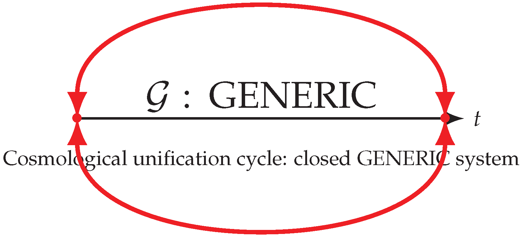
Table 2.
Entropy channels and their physical interpretation in the controller framework.
| Symbol | Channel | Physical meaning | Controller interpretation |
|---|---|---|---|
| Matter | Local microscopic entropy production (particle creation, field interactions). | Internal source | |
| Dissipative (bulk, viscous, etc.) | Irreversible entropy due to macroscopic non-equilibrium; acts as an internal correction term. | Internal correction | |
| Horizon | Geometric entropy from the cosmological boundary (Bekenstein–Hawking term). | External sink or source |
Disclaimer/Publisher’s Note: The statements, opinions and data contained in all publications are solely those of the individual author(s) and contributor(s) and not of MDPI and/or the editor(s). MDPI and/or the editor(s) disclaim responsibility for any injury to people or property resulting from any ideas, methods, instructions or products referred to in the content. |
© 2025 by the authors. Licensee MDPI, Basel, Switzerland. This article is an open access article distributed under the terms and conditions of the Creative Commons Attribution (CC BY) license (http://creativecommons.org/licenses/by/4.0/).
Copyright: This open access article is published under a Creative Commons CC BY 4.0 license, which permit the free download, distribution, and reuse, provided that the author and preprint are cited in any reuse.


