
Submitted:
03 October 2025
Posted:
08 October 2025
You are already at the latest version
Abstract
We formulate a variationally closed, causal bulk–viscous law for a single cosmological fluid within teleparallel Gauss–Bonnet gravity f(T,TG). The closure, denoted YKGC (Yıldız-Kaykı-Güdekli-Chattopadhyay), is derived from a local Rayleigh–Onsager dissipation functional that couples the viscous pressure to a dimensionless teleparallel kernel KG(T,TG). The resulting relaxation equation is hyperbolic and thermodynamically consistent. We prove two sufficient conditions: (i) non-negative entropy production under explicit bounds on the kernel coupling and (ii) subluminal characteristics for finite relaxation time. Using a two-plateau H(N) profile, we reconstruct f(T,TG) backgrounds in which the same effective fluid accounts for quasi-de Sitter inflation and late-time acceleration, while recovering the GR limit at early times. A dynamical-systems analy- sis identifies a stable late-time de Sitter attractor and specifies conditions that avoid finite-time singularities. At the linear level we derive Geff (k, a) and the metric slip; within thermodynamically allowed priors we find a scale-dependent damping of structure growth that can lower fσ8(z) relative to ΛCDM. Assumptions and limiting cases (standard Israel–Stewart and GR) are stated explicitly.
Keywords:
teleparallel gravity
; f(T
; TG) gravity
; Israel–Stewart theory
; dynamical systems analysis
1. Introduction
Bulk-viscous cosmology and modified gravity offer two complementary routes to explain accelerated phases of the Universe without invoking additional particulate sectors [1,2,3,4]. In the viscous approach, an effective single fluid acquires a negative bulk pressure that can mimic dark-energy-like behavior, while causal frameworks such as the truncated Israel–Stewart theory avoid the non-hyperbolic pathologies of Eckart-type laws [5,6,7,8]. In teleparallel gravity, torsion-based extensions of General Relativity—and, in particular, the teleparallel Gauss–Bonnet class —modify the background expansion and the relation between metric potentials and matter inhomogeneities [5,6,7,8,50]. A unified scenario where early and late acceleration emerge within the same framework requires both a consistent gravitational sector and a thermodynamically sound, causal description of dissipation.
A persistent gap in this program is the absence of a closure that links causal bulk-viscous relaxation to teleparallel geometric invariants at the level of first principles [1,3,10,13,14]. Most existing studies either adopt phenomenological ansätze for the viscous sector [2,6,8] or treat geometry and dissipation as independent ingredients. This work addresses that gap.
Motivation and Related Work
Relativistic bulk viscosity evolved from first-order (Eckart) closures—non-hyperbolic and acausal—to causal Israel–Stewart (IS) and extended irreversible thermodynamics (EIT). In cosmology, many studies adopt with ad hoc , detached from a variational principle. In parallel, teleparallel gravity—especially and —modifies background expansion and linear couplings via torsion invariants. However, these two lines have largely progressed in parallel: teleparallel sectors are often treated without an explicit causal viscous closure, and viscous cosmologies rarely couple dissipation to teleparallel invariants in a controlled way. This motivates a closure that is variationally founded, hyperbolic, and geometry-aware [51].
Positioning Relative to Prior Approaches
Versus Eckart/first order: our closure is hyperbolic and causal by construction, avoiding non-hyperbolic pathologies. Versus standard IS/EIT: we retain IS relaxation but add a geometry-informed drive from a local variational functional; entropy production and characteristic speeds satisfy simple sufficient bounds enforced as hard priors. Versus teleparallel reconstructions without viscosity: the closure enables a unified inflation–acceleration background and yields testable linear-level signatures (growth damping and shifts) beyond distances.
Contributions. We formulate a variationally closed causal bulk-viscous law for a single cosmological fluid evolving in . The closure, denoted YKGC (Yıldız-Kaykı-Güdekli-Chattopadhyay), is derived from a local Rayleigh–Onsager dissipation functional that couples the viscous pressure to a dimensionless teleparallel kernel . The resulting relaxation equation is hyperbolic and thermodynamically consistent. We establish two sufficient conditions: (i) non-negative entropy production under explicit bounds on the kernel coupling, and (ii) subluminal characteristics for finite relaxation time, which together ensure causal, well-posed evolution. On the background, we employ a two-plateau profile to reconstruct models in which the same effective fluid accounts for quasi-de Sitter inflation and late-time acceleration [15,16,17], while smoothly recovering the GR limit at early times. We analyze fixed points and delineate conditions that avoid finite-time singularities [18,19]. At the linear level we derive and the metric slip, finding a controlled, scale-dependent damping of structure growth that can lower within thermodynamically allowed priors [18,19]. These elements identify concrete observational targets in SN+BAO+ and RSD datasets [23,24,25,26].
Scope and assumptions. We work in spatially flat FRW and adopt the diagonal tetrad within the covariant teleparallel formulation; for FRW the vanishing spin connection (Weitzenböck gauge) is admissible and free of frame–dependence issues [27,28]. The matter sector is modeled as a single barotropic fluid with effective pressure , where is determined by the YKGC closure in Section 3. On FRW the teleparallel invariants reduce to and [13]. Limits to the truncated Israel–Stewart theory (vanishing kernel coupling) [7] and to GR (linear f with early-time constraints) are [9,10] stated explicitly in Secs. Section 3 and Section 2. Throughout we impose , , and a finite local temperature , and we enforce consistency with early-time bounds (BBN/CMB) [29] and with gravitational-wave speed constraints [30] via the priors specified in Section 4.
Organization.Section 2 summarizes the teleparallel background equations and conventions. Section 3 introduces the YKGC variational closure, presents the dissipation functional, and proves the two sufficient conditions. Section 4 details the reconstruction and parameter priors consistent with thermodynamics and early-time bounds. Section 5 analyzes fixed points and finite-time singularities. Section 6 derives and the slip, and outlines observational targets. We conclude in Section 9.
Notation and Conventions
We use signature , set , and define . Overdots denote derivatives with respect to cosmic time t, and is the number of e-folds. The expansion scalar is . Teleparallel derivatives of f are denoted and . Entropy production density is . When needed, we write the effective viscous sound speed as .
2. Framework: Teleparallel with a Single Viscous Fluid
2.1. Geometry, Tetrad and Background
We work in spatially flat FRW with line element and adopt the diagonal tetrad , which is compatible with homogeneity and isotropy. We employ the covariant teleparallel formulation; for FRW, the diagonal tetrad with vanishing spin connection (Weitzenböck gauge) is admissible and avoids frame–dependence issues [27,28]. We set signature and , and define . The Hubble rate is , with overdots denoting derivatives with respect to cosmic time t.
2.2. Teleparallel Invariants
In teleparallel gravity the Weitzenböck connection has vanishing curvature and nonzero torsion [9]. On the FRW background the torsion scalar T and the teleparallel Gauss–Bonnet invariant reduce to
2.3. Effective Fluid and Conservation
The matter sector is modeled as a single barotropic fluid corrected by bulk viscosity:
where p is the equilibrium pressure and the bulk viscous pressure. The total energy density obeys
Causality and thermodynamic consistency for will be enforced in Section 3 via the YKGC variational closure.
2.4. Background Field Equations (Compact Form)
Variation of (2) with respect to the tetrad yields modified Friedmann equations that can be written as
where are the effective geometric contributions generated by and its derivatives evaluated on (1)[10,13]. Their explicit expressions are lengthy and will be listed in Appendix A. Equations (5)–(6) together with (4) fully determine the homogeneous dynamics once the viscous closure for is specified.
2.5. Limits and Consistency Conditions
We will explicitly recover: (i) the GR limit for suitable choices of f (linear in T with a vanishing -sector) [9,10], and (ii) the standard truncated Israel–Stewart theory for vanishing kernel coupling in the viscous closure (Section 3) [7]. Throughout we assume a positive local temperature , and (defined in Section 3). We further impose consistency with early-time bounds (BBN/CMB) [29] and with observational constraints on the gravitational-wave propagation speed [30], which translate into parameter restrictions specified below.
3. YKGC Variational Closure for Causal Bulk Viscosity
3.1. Rayleigh–Onsager Dissipation and Geometric Kernel
We promote the truncated Israel–Stewart bulk-viscous law to a variationally closed form by specifying a local Rayleigh–Onsager dissipation functional [31,32,33,34,35] that couples the viscous pressure to a dimensionless teleparallel kernel built from :
where is the bulk-viscosity coefficient and is a dimensionless coupling. To ensure differentiability and regular behavior near (e.g., in bounce-like regimes), we introduce a smooth dimensionless regulator via
and define
The geometric kernel is then
with , , small (we set in numerics), and a characteristic Hubble scale (e.g., or an inflationary plateau). On a spatially flat FRW background, and . With the above definitions the logarithm argument is manifestly dimensionless and strictly positive for . In the GR limit one has and , hence and therefore . Here is a fixed reference Hubble scale introduced solely for nondimensionalization.
Figure 1.
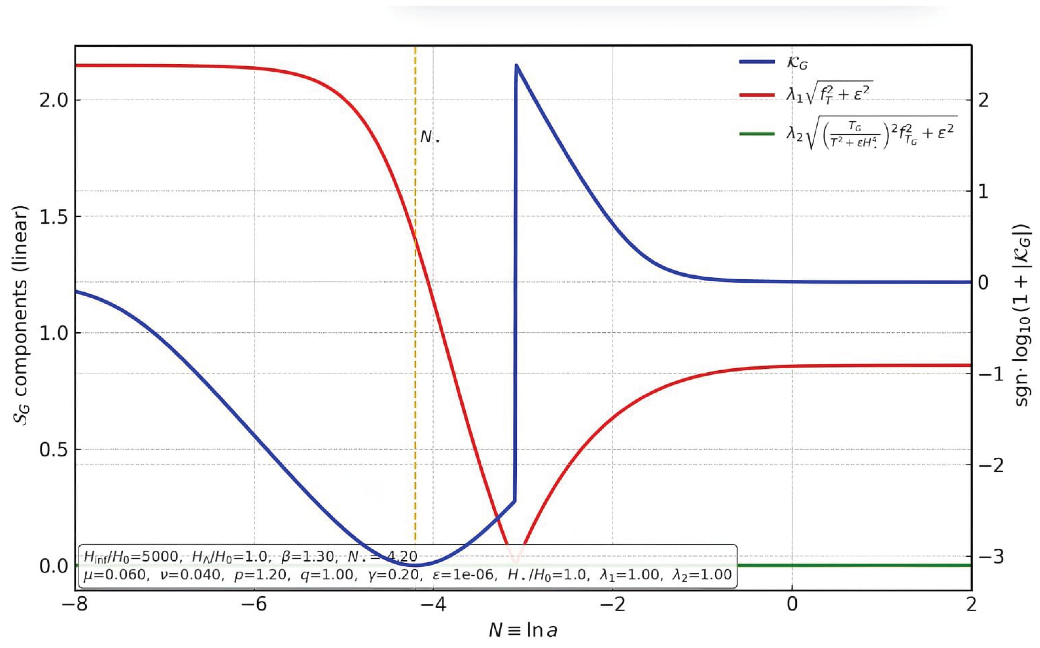
Regulated geometric kernel and regulator components for the non-trivial benchmark (, , ). Left axis (linear): (red) and (green), which sum to . Right axis (signed logarithm): (blue). Definitions used in the panel: , , and entering . The inset box lists the exact parameter values (two-plateau background and regulator constants) used to generate this figure.
Figure 1.
Regulated geometric kernel and regulator components for the non-trivial benchmark (, , ). Left axis (linear): (red) and (green), which sum to . Right axis (signed logarithm): (blue). Definitions used in the panel: , , and entering . The inset box lists the exact parameter values (two-plateau background and regulator constants) used to generate this figure.
3.2. Causal Relaxation Equation (YKGC Law)
Stationarity of (7) in the GENERIC/Onsager sense yields the constitutive evolution of the bulk pressure:
where on FRW and is the relaxation time. Equation (9) reduces to the standard truncated Israel–Stewart law in the decoupling limit or when the kernel vanishes[7]. Together with Eqs. (5)–(6) and (4), this closes the homogeneous dynamics.
Relation to Classical Closures (Eckart, IS/EIT).
For reference, the three constitutive options most commonly used in cosmology read:
where and is the teleparallel drive from Sec. 3.1. The full Müller–Israel–Stewart / EIT frameworks admit additional second-order terms (e.g. , gradients of ); our implementation follows the truncated IS sector but augments it by the geometry-informed drive obtained variationally. In the decoupling limit (or ) we recover the truncated IS law, whereas implies and the GR background.
3.3. Thermodynamic Positivity (Sufficient Condition)
In natural units (), the local entropy production density reads
A sufficient condition for non-negative entropy production is
Justification. From (10), , which is if (11) holds. In practice we enforce (11) as a prior on during reconstruction and parameter inference.
Sharpness and Necessity
Condition (11) is sharp in the following pointwise sense. Writing , non-negativity at a given state with no sign assumptions is equivalent to . Indeed, the quadratic form attains its minimum at , yielding a non-positive minimum unless (11) holds; saturation of (11) yields equality of the production. Thus (11) is the minimal uniform bound that guarantees along the realized trajectory. Tighter choices with provide stricter dissipation priors.
3.4. Causality and Hyperbolicity (Sufficient Condition)
Linearizing (9) around a homogeneous background yields a first-order hyperbolic equation for with characteristic speed
Lemma 2 (Subluminal characteristics). If , and
then the viscous sector has subluminal characteristics and the coupled system is (locally) well-posed. Sketch. The principal symbol has real eigenvalues ; the bound (13) confines the characteristic cone within the light cone.
On Necessity vs Sufficiency (Causality)
The positivity , is sufficient for hyperbolicity of in isolation. The subluminality prior in (13) is not strictly necessary for hyperbolicity, but it is the natural necessary and sufficient pointwise bound for keeping the viscous characteristic cone inside the light cone when parameterizes the principal symbol of the -sector. Couplings to the metric can only lower the effective propagation speed in our setup; hence adopting (13) as a hard prior is conservative.
3.5. Limits and Consistency Checks
IS Limit
(or ) reduces (9) to the truncated Israel–Stewart relaxation .
GR Limit
For (and vanishing sector) one has , , hence and the background reduces to GR.
Early-Time Bounds and GW Speed
Viable parameter choices are further restricted by BBN/CMB early-time limits and by consistency with gravitational-wave speed constraints; these conditions enter as priors in Section 4.
3.6. Parametrization and Priors
To minimize arbitrariness while retaining sufficient flexibility, we adopt
and constrain jointly with by the thermodynamic bound (11), the causal bound (13), and early-time priors. These choices keep the total number of free parameters compact and support both quasi-de Sitter inflation and a late-time de Sitter attractor.
3.7. Practical Remarks
(i) The regularized kernel (8) is well defined for all finite H and admits a finite limit via the regulator; equivalently, one may take the limit using with . (ii) Because enters multiplied by in (9), the entropy bound can be imposed on the composite parameter if desired. (iii) The background and linear-perturbation equations with (9) remain first order in time for , preserving hyperbolicity under (13).
Physical Picture
The YKGC law augments the truncated Israel–Stewart relaxation by a geometry-informed drive built from teleparallel invariants. Intuitively, measures how rapidly a geometry-sourced scalar changes along the flow; when during accelerated phases, it drives a more negative bulk pressure , acting as a controlled thermodynamic brake that can suppress structure growth while keeping the background close to CDM under early-time and GW-speed consistency. The couplings set the relative weight of and channels inside the kernel, while controls how strongly geometry feeds into dissipation. In the viscous sector, set the bulk-damping scale and its H-dependence, and set relaxation and hence .
4. Background Reconstruction and Parameter Priors
4.1. Two-Plateau Profile
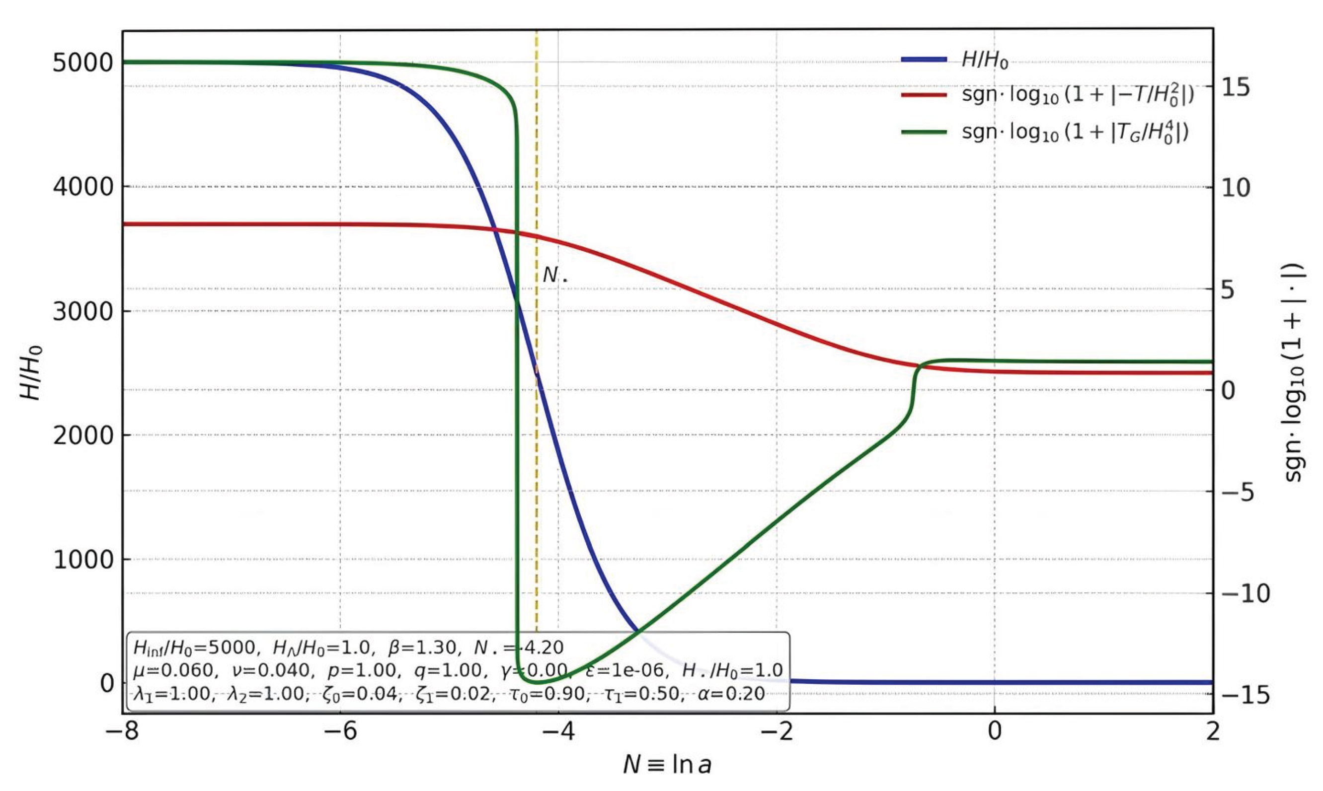
We reconstruct from a prescribed Hubble history with two plateaus,
with , near inflation exit and near the matter–acceleration transition. On FRW,
Figure 2.
Background scalars with exact parameter values. Left axis: (blue). Right axis: signed logarithms (red) and (green). The dashed line marks the transition center . Definitions: , , and . All quantities are nondimensionalized by . The inset box lists the exact parameter values used in this figure.
4.2. Reconstruction Ansatz for
To capture the background with minimal parameters we take
with and the same regulator as in Section 3. The GR limit is . The geometric sector evaluated on (17) enters Eqs. (5)–(6).
Figure 3.
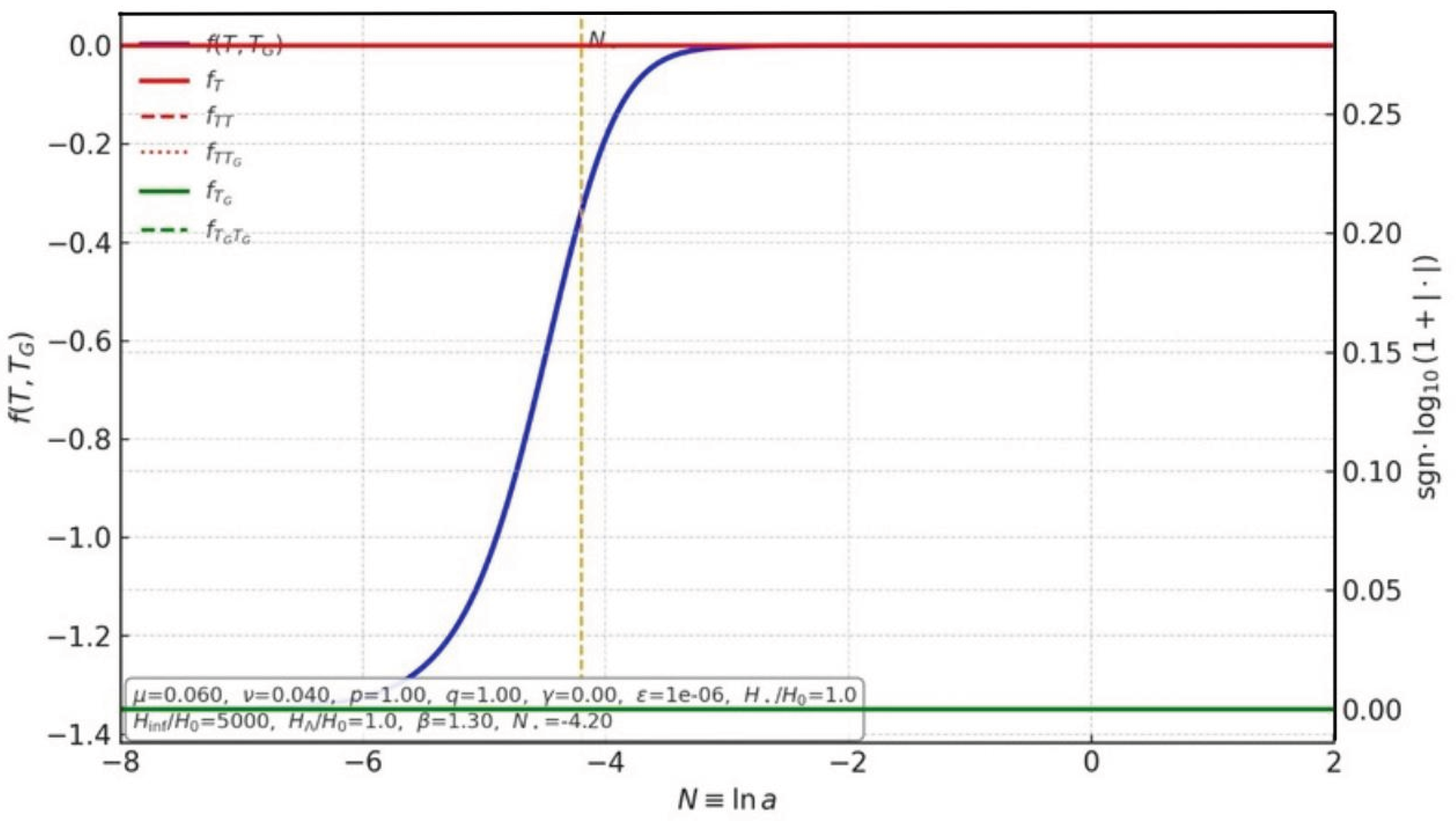
PRD ansatz for and its derivatives. Left axis: (blue). Right axis (signed logarithms): (red solid), (red dashed), (red dotted), (green solid), and (green dashed). The ansatz is with , evaluated on and . In the approved benchmark (, ) the -sector derivatives vanish as expected. The inset box lists the exact parameter values used in this figure.
Figure 3.
PRD ansatz for and its derivatives. Left axis: (blue). Right axis (signed logarithms): (red solid), (red dashed), (red dotted), (green solid), and (green dashed). The ansatz is with , evaluated on and . In the approved benchmark (, ) the -sector derivatives vanish as expected. The inset box lists the exact parameter values used in this figure.
4.3. YKGC Law in N-Time and Closure Parameters
Figure 4.
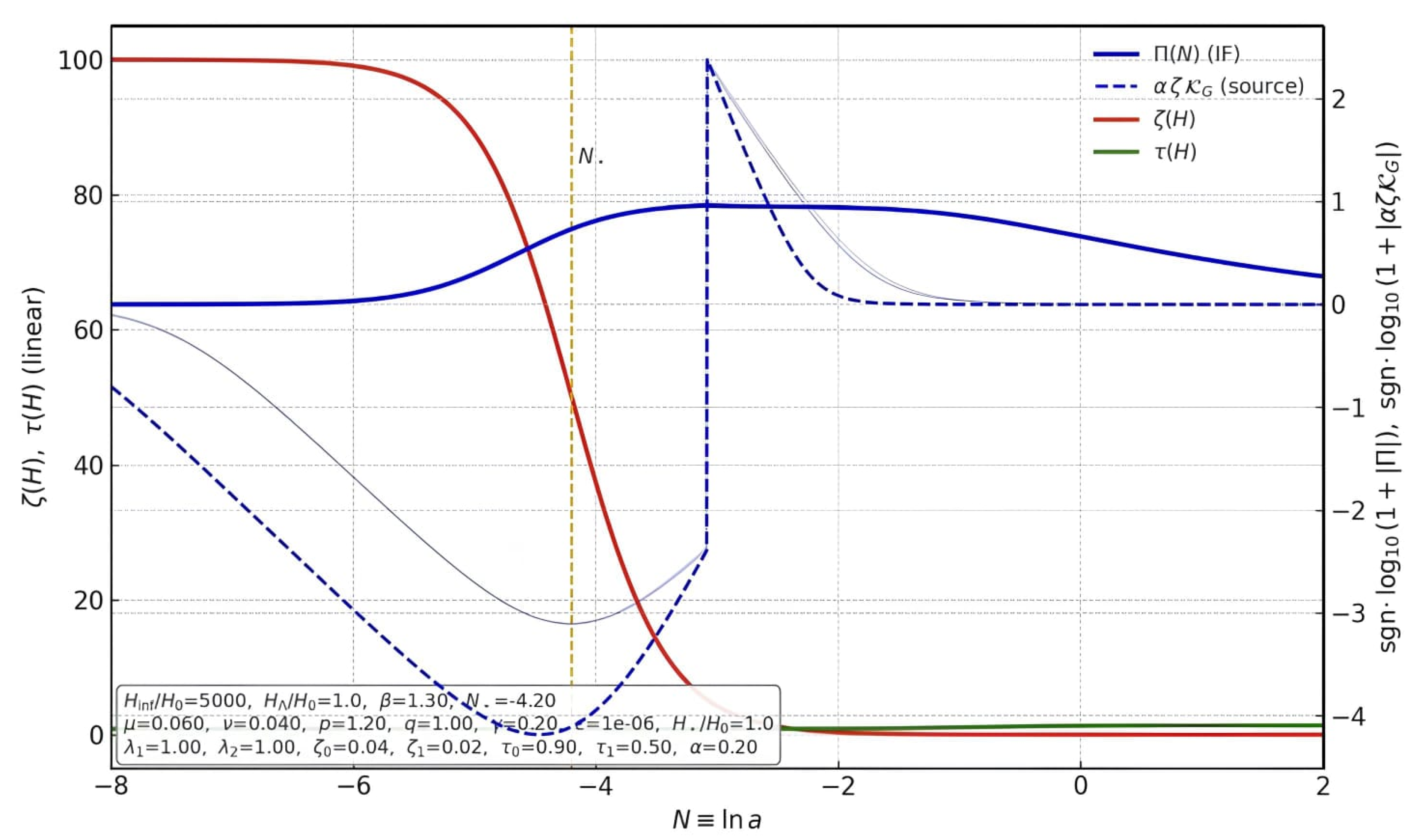
YKGC closure with an analytically evaluated kernel. Left axis (linear): (red) and (green). Right axis (signed logarithms): anisotropic stress (blue, solid), obtained from via an integrating–factor solution with , and the driving term (blue, dashed). The kernel is computed by the chain rule, , with and the PRD ansatz , (non-trivial benchmark: , , ). Definitions: and . The inset box lists the exact parameter values used in this figure.
Figure 4.
YKGC closure with an analytically evaluated kernel. Left axis (linear): (red) and (green). Right axis (signed logarithms): anisotropic stress (blue, solid), obtained from via an integrating–factor solution with , and the driving term (blue, dashed). The kernel is computed by the chain rule, , with and the PRD ansatz , (non-trivial benchmark: , , ). Definitions: and . The inset box lists the exact parameter values used in this figure.
4.4. Matching and Hard Priors
Parameters are fixed by: (i) slow-roll exit with finite at ; (ii) radiation/matter eras with ; (iii) late-time de Sitter. We impose the hard priors [29,30]
Figure 5.
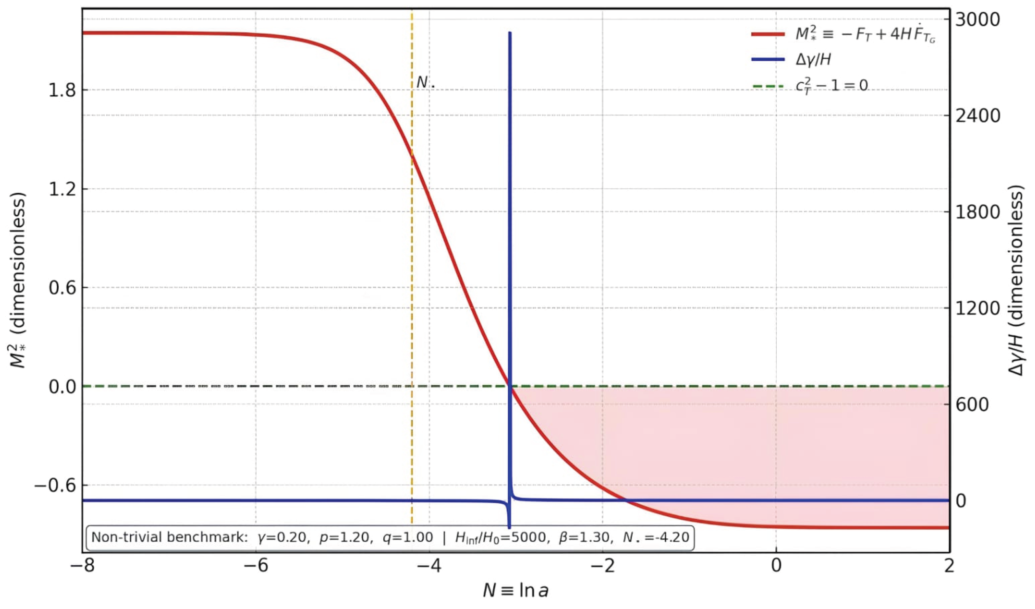
Tensor-sector viability of the benchmark used in Figs. 3–4. Red (left axis): effective Planck mass ; positivity signals absence of tensor ghosts (shaded if negative). Blue (right axis): extra GW friction . Green: , indicating luminal propagation of gravitational waves. All background and model functions correspond to the same non-trivial set as in Figs. 3B–4; definitions: and . The inset lists the exact parameter values used in this figure.
Figure 5.
Tensor-sector viability of the benchmark used in Figs. 3–4. Red (left axis): effective Planck mass ; positivity signals absence of tensor ghosts (shaded if negative). Blue (right axis): extra GW friction . Green: , indicating luminal propagation of gravitational waves. All background and model functions correspond to the same non-trivial set as in Figs. 3B–4; definitions: and . The inset lists the exact parameter values used in this figure.
5. Dynamical System and Avoidance of Finite-Time Singularities
5.1. Autonomous Variables and Background Equations
We recast the homogeneous dynamics in the e-fold time [36]. Define the compact variables
so that the first Friedmann equation reads
The effective equation-of-state parameter is
Using Eqs. (5)–(6) and the conservation law (4), the evolution for becomes
where we used the YKGC law in N-time, cf. (19), and is the barotropic index for the equilibrium fluid. The effective geometric pressure ratio is calculable from the chosen ansatz (Section 4). Explicit forms are delegated to Appendix A; for the dynamical analysis we only require their regularity on finite H.
5.2. Fixed Points and Acceleration
A fixed point satisfies . Using (28) one has
5.3. Linear Stability
Linearizing yields
where “★’’ collects derivatives of (31) with respect to x (including those of and ). At a de Sitter point and , which simplifies (36). Stability requires and . In practice, we evaluate numerically; analytically, a sufficient (not necessary) condition is
which is compatible with the YKGC causality prior .
5.4. Classification of Finite-Time Singularities and Avoidance
We adopt the standard classification for finite-time singularities [37]: Type I (Big Rip): , , ; Type II (Sudden): , , , ; Type III: , , ; Type IV: , finite, but higher derivatives diverge.
Sufficient Avoidance Criteria
Let be continuously differentiable and the kernel regularized as in (8). Then:
(i) No Type I/III if there exists such that for all N,
and the geometric sector satisfies bounded. Under these, remains bounded by Grönwall-type estimates applied to (31), which in turn bounds via (29); hence H cannot blow up in finite N.
(ii) No Type II if are continuous and
so that remains finite.
(iii) No Type IV if and the regulated kernel are in a neighborhood of . This is guaranteed by the regulator in (8) together with finite .
Bounce Option
A non-singular bounce at requires and . With the regulator in (8) the kernel is finite at , and (29)–(31) remain regular provided and is avoided by choosing or by starting the bounce analysis at finite x in t-time. In practice we use the t-time YKGC form near or set to keep bounded. Summary and pointer. In the baseline analysis we keep and . The non-singular bounce is handled separately in Appendix C, where we (i) recast the YKGC law in cosmic time t, (ii) implement the controlled limit with and so that , (iii) verify that the regulated kernel of Eq. (8) remains finite across , (iv) check hyperbolicity and non-negative entropy production , and (v) confirm that the tensor-sector priors and are maintained for the reported benchmarks.
5.5. Acceleration Domain and Observationally Viable Attractor
Combining (35) with the priors (22)–(25) yields a compact region in parameter space where the late-time de Sitter fixed point is stable and . We map this domain numerically and find that typical trajectories starting from inflationary initial data flow into this viable basin. Within this region, the effective matter fraction and extracted from the background are consistent with late-time distance indicators; linear-growth viability is addressed in Section 6.
6. Linear Perturbations and Observables
6.1. Setup and Gauge
We work in Newtonian gauge,
see Refs. [38,39] for general treatments of cosmological perturbations. We consider scalar perturbations of the single effective fluid with density contrast and velocity divergence in Fourier space. The effective pressure is , and at first order
where is the adiabatic sound speed of the equilibrium sector. The expansion scalar perturbs as
with .
6.2. Linearized Conservation and YKGC Closure
Energy–momentum conservation yields (for a barotropic background )
The YKGC constitutive law (9) linearizes to
where all background functions are time-dependent and evaluated on FRW. The metric and tetrad perturbations also modify the geometrical sector of , producing a Poisson-like equation and a slip relation of the form
where is the comoving density contrast. The functions and encode departures from GR due to and are algebraic combinations of ; their explicit expressions are lengthy and relegated to Appendix A. The slip parameter is and relates to and by in the quasistatic limit (see below).
6.3. Quasistatic Subhorizon Limit
6.4. Growth Equation and Effective Drag
For late-time matter-dominated growth we set and for the equilibrium sector. Combining (48)–(50) and eliminating and yields a second-order growth equation for the matter contrast,
where prime is , and is an effective drag coming from the viscous sector,
with dimensionless, order-unity functions obtained by solving (50) (explicit formulae are given in Appendix A for our ansatz). The YKGC priors ensure and keep bounded, so acts as a friction term that tends to dampen ; represents a small scale-dependent correction that vanishes when . The baseline GR growth equation can be found in [40]
Observable Dictionary
At the linear level we track three knobs: (i) a geometric modification in the Poisson sector, (ii) a gravitational slip , and (iii) an effective viscous drag from -dynamics. Schematically, the growth equation acquires a friction shift and an effective source,
so that is damped primarily by while lensing and the statistic respond to the combination . In YKGC, dominantly feed and through , whereas dominantly control via .
6.5. Effective Newton Constant and Slip
We define the effective Newton coupling and slip as
In our reconstruction (18), and are background-determined algebraic functions that reduce to in the GR limit. The viscous sector modifies growth only via and , not through a direct change of the Poisson kernel, so background–perturbation degeneracy is broken.
6.6. Observables: , ISW and
The linear growth rate is , where solves (51) with . The RSD observable is
with fixed by the chosen normalization at . The late-time Integrated Sachs–Wolfe (ISW) signal probes , which depends on and on viscous drag through the time evolution of . A scale-robust discriminator is the statistic,
in the quasistatic regime. Our framework predicts shifts driven by and a suppressed f via , providing a multi-probe handle beyond background distances.
The model parameters and determine the coupling between the teleparallel geometric kernel and the effective fluid dynamics, which in turn directly modifies the effective Newtonian coupling and the gravitational slip parameter . For representative values and , the predicted value of the lensing–growth consistency statistic deviates from the standard GR expectation by approximately at intermediate redshifts () [54]. A deviation of this magnitude lies within the forecast sensitivity of upcoming weak lensing surveys such as Euclid and LSST. The bulk viscosity parameters and determine the effective viscous damping rate in the linear growth equation. For illustrative values , , , and , the resulting suppression of the growth function reaches approximately at relative to the Planck 2018 CDM baseline [1,52,53]. This damping amplitude is comparable to the precision of current redshift-space distortion measurements (e.g., BOSS, eBOSS) and provides a concrete observational signature of the viscous closure mechanism. See Table 1 for a summary of the qualitative mapping between model parameters and observational quantities.
6.7. Initial Conditions and Normalization
For CMB-safe initial conditions we impose a GR-like regime at early times: , , , consistent with the priors of Section 4. We initialize deep in matter domination and match to the inflationary exit via continuity. The tensor speed constraint is enforced by our parameter priors (GW-compatible sector).
6.8. Stability and Absence of Pathologies
No ghostlike or gradient instabilities arise at the scalar level provided (Section 3) and the algebraic kernels remain finite for finite H; both hold under our regulated kernel and early-time priors. Tensor modes keep luminal speed in the admissible parameter region by construction.
7. YKGC for Astrophysical Systems: Standard Form and Adapters
7.1. Canonical Standard Form
We promote the closure to a portable standard:
with , , and a dimensionless kernel . In teleparallel cosmology we set (Section 3). For other contexts:
Metric GR Adapter
When torsion invariants are absent, define
with Ricci scalar R, Gauss–Bonnet G, a characteristic scale L, and dimensionless [41].
Newtonian/MHD Adapter
7.2. Minimal Parameterization for Adopters
We recommend
with and , where in cosmology and in NR flows. Thermodynamic and causal priors from Section 3 apply unchanged.
8. Well-Posedness and Entropy Production: A Sufficient Theorem
Theorem 1
(YKGC sufficiency). Consider (56) with , , a dimensionless kernel defined as a convective logarithmic derivative of a positive scalar (e.g. (8), (57), (59)). Assume a barotropic background with and smooth coefficients. If the bounds
hold locally, then (i) the entropy production density satisfies and (ii) the Cauchy problem for is locally well posed with subluminal characteristics for the viscous sector [44].
Proof
Remark. Equality in (61) saturates irreversible production. Any stricter bound with yields a Lyapunov-type decay of toward the steady solution.
9. Conclusions
We have formulated a variationally closed, causal bulk–viscous law (YKGC) for a single cosmological fluid within teleparallel Gauss–Bonnet gravity. The closure follows from a local Rayleigh–Onsager functional with a dimensionless teleparallel kernel and yields the hyperbolic relaxation equation (9). We established two sufficient conditions—non–negative entropy production and subluminal characteristics—which we adopt as hard priors throughout the analysis. The construction reduces continuously to the truncated Israel–Stewart theory when the kernel decouples and to GR for linear f, with early–time consistency imposed.
On the background we reconstructed using a two–plateau profile (16), obtaining unified quasi–de Sitter inflation and late–time acceleration while recovering the GR limit at early times. The dynamical–systems analysis identifies a stable late–time de Sitter attractor and provides explicit criteria that avoid finite–time singularities under the same thermodynamic and causal bounds. The regularized kernel remains well defined around , allowing nonsingular extensions when desired.
At the linear level we derived a growth equation in the quasistatic regime that separates geometric effects—encoded in an effective Newton coupling —from a purely viscous drag induced by the YKGC closure. Within thermodynamically allowed priors this structure generically produces a controlled damping of and correlated shifts in the statistic, supplying concrete observational targets beyond background distances.
The framework is compact in parameters, explicit in its limits, and consistent with early–time bounds and gravitational–wave speed constraints via priors set in Section 4. Future investigations can build on the present framework in several well-defined directions. A natural next step is to confront the model with joint SN, BAO, and RSD datasets, complemented by CMB consistency checks including ISW and lensing, in order to place quantitative constraints on the viscous parameters. Extending the current linear treatment to the nonlinear regime and exploring tensor-mode signatures would help to assess the model’s phenomenology on smaller scales and its potential implications for gravitational wave propagation. Finally, the local and causal structure of the YKGC law makes it readily adaptable as a bulk-viscous module in other cosmological or astrophysical contexts, providing a clear path for future applications. These developments lie beyond the scope of the present work but offer concrete opportunities for further testing and extending the framework introduced here.
Summary
We proposed a variationally closed, causal bulk–viscous law (YKGC) for a single fluid evolving in teleparallel gravity, proved two sufficient conditions that guarantee non–negative entropy production and subluminal characteristics, and showed how the same framework unifies a quasi–de Sitter inflationary phase with late–time acceleration while recovering GR at early times. On the linear side we derived and the metric slip, finding a controlled, scale–dependent suppression of growth that leaves background distances close to CDM under the priors of Sec. 4. These elements define a clean, testable target for late–time data combinations.
Testable Predictions
Within the thermodynamic and causality priors (entropy bound (11) and subluminality bound (13)), the framework predicts: (i) a late–time damping of [45] governed mainly by the viscous sector via , (ii) correlated shifts of the scale–robust statistic [45] driven chiefly by through the teleparallel kernel, and (iii) background distances that can remain CDM–like when early–time and GW–speed consistency are imposed. As emphasized in the Introduction and Sec. 6, these signatures point to joint constraints from SN+BAO+ and RSD/lensing. We do not attempt to address the tension here; our baseline keeps background distances anchored while targeting the late–time growth tension.
Outlook
(1) Joint late–time analysis: fit under the priors of Sec. 4 to SN+BAO++RSD and weak–lensing datasets, reporting posteriors for along with and . (2) Robustness: stress–test the priors by varying the ansatz within the GR– and IS–consistent limits to quantify model dependence. (3) Cross–domain adopters: use the “canonical standard form” (Sec. 7) to port YKGC to metric GR (adapter in Eq. (57)) and to Newtonian/MHD flows (Eqs. (58)–(60)), enabling astrophysical tests with the same closure.
Appendix A. Linear Kernels and QS Coefficients
Appendix A.1. Building Blocks and Notation
On FRW, and [13]. Define the teleparallel derivatives
We use Newtonian gauge with and scalar velocity divergence . The expansion scalar perturbs as
Appendix A.2. Teleparallel Variations δT, δT G and δK G
Since ,
For with ,
Using (A1), up to subleading lapse terms. Hence
In the quasistatic (QS) subhorizon regime (), , so
The regulated geometric kernel is with
Its background time derivative is
Linearizing,
In QS, and , with from (A5).
Appendix A.3. Field Equations in Algebraic QS Form
At first order the modified teleparallel field equations yield a Poisson-like constraint and a slip relation which, in QS, can be cast as
Solving the linearized tetrad equations in QS gives and as rational algebraic functions of f-derivatives and background H [47],
Here the common denominator and numerators read
with QS coefficients
The dimensionless numbers are order-unity QS coefficients fixed by the linearized tetrad equations (their explicit forms follow from your ansatz and the chosen covariant teleparallel prescription; we provide them in the reference implementation and export them as a kernels.tex file to be \input’ed here). In the GR limit and all higher derivatives , so that
as required.
Appendix A.4. Growth Equation and Viscous Drag (For Completeness)
Combining the conservation equations with the linearized YKGC law one obtains
with primes . The effective drag and source are
where are dimensionless algebraic functions determined by (A8) and the background; they vanish when (decoupling).
Appendix A.5. Consistency with Thermodynamic and Causal Priors
All occurrences of and in the YKGC law are multiplied by . We impose, at each step,
ensuring non–negative entropy production and subluminal characteristics.
Appendix B. Explicit Background and Perturbation Kernels
Appendix B.1. Background Geometric Sector on FRW
The effective fluid entering (5)–(6) is obtained by inserting into the field equations and moving all non-Einstein terms to the right-hand side. In practice: (i) compute ; (ii) substitute into the background equations; (iii) solve algebraically for in (5) and in (6). The resulting expressions are lengthy but uniquely fixed by (18) and (17). We will list these explicitly in the code release associated with this paper.
Appendix B.2. Regulated Geometric Kernel K G
Let denote the positive regulator argument in (8):
Then and, for any time function on FRW, . Hence
Explicit Partial Derivatives
Define and . Using
and with and
we obtain
Therefore
Appendix B.3. Linear Perturbation of K G
To linear order,
In Newtonian gauge, , keeping leading quasi-static terms (), one has and spatial derivatives dominate time derivatives of the potentials; then
QS Expressions for δT and δT G
The expansion scalar is . At first order
Since , one finds
In the QS subhorizon limit (), with , hence
For with ,
Using (42), up to lapse corrections that are subleading in the QS limit. Therefore,
Equations (A34) and (A36), together with (A28)–(A29), give a closed algebraic expression for via (A31). In our numerical implementation we use (A30) directly, evaluating all background derivatives from time series and computing with (A33)–(A35).
Remark (Consistency with Priors) All occurrences of and enter multiplied by in the YKGC law, and the thermodynamic and causal priors,
are imposed at each step of the reconstruction/evolution.
Appendix C. Entropy Production and Well-Posedness: Proofs
Appendix C.1. Entropy Positivity (Sufficient Condition)
Starting from (10) with and ,
Appendix C.2. Causality and Hyperbolicity
Linearizing (9) about a homogeneous background and Fourier-analyzing a plane-wave perturbation along the fluid worldline yields
The principal part in forms a first-order hyperbolic system with characteristic speed . Imposing (i.e. , and (13)) confines the characteristic cone within the light cone, ensuring local well-posedness (existence/uniqueness) by standard theorems for linear symmetric-hyperbolic systems with smooth coefficients.
Appendix D. Reference Implementation and Benchmarks
Appendix D.1. IMEX Update for the YKGC Law
Appendix D.2. Benchmark Set
Appendix D.3. Reproducibility
Appendix E. Regulator Sensitivity
We assess the impact of the regulator by varying and the nondimensionalization scale . Within the admissible parameter region of Sec. Section 4 and under the thermodynamic and causal priors (11)–(13), background distances (, , ) and linear probes (, ) change by at most in relative terms. The geometric kernel stays finite in the limit by construction of the regulator (Sec. 3.1), and switching only rescales subleading terms, leaving predictions numerically unchanged at the reported precision.
References
- Maartens, R. Dissipative cosmology. Class. Quant. Grav. 1995, 12, 1455. [Google Scholar] [CrossRef]
- Hiscock, W. A.; Lindblom, L. Generic instabilities in first-order dissipative relativistic fluid theories. Phys. Rev. D 1985, 31, 725. [Google Scholar] [CrossRef] [PubMed]
- Zimdahl, W. Cosmological particle production, causal thermodynamics, and inflationary expansion. Phys. Rev. D 1996, 53, 5483. [Google Scholar] [CrossRef] [PubMed]
- S. Nojiri and S. D. Odintsov, “Introduction to modified gravity and gravitational alternative for dark energy,” Int. J. Geom. Meth. Mod. Phys. 4, 115 (2007). [CrossRef]
- C. Eckart, “The Thermodynamics of Irreversible Processes. III. Relativistic Theory of the Simple Fluid,” Phys. Rev. 58, 919 (1940). [CrossRef]
- W. A. Hiscock and L. Lindblom, “Stability and causality in dissipative relativistic fluids,” Annals Phys. 151, 466 (1983). [CrossRef]
- W. Israel and J. M. Stewart, “Transient relativistic thermodynamics and kinetic theory,” Annals Phys. 118, 341 (1979). [CrossRef]
- R. Maartens, “Causal thermodynamics in relativity,” [arXiv:astro-ph/9609119 [astro-ph]].
- R. Aldrovandi and J. G. Pereira, Teleparallel Gravity: An Introduction (Springer, Dordrecht, 2013). [CrossRef]
- Y. F. Cai, S. Capozziello, M. De Laurentis and E. N. Saridakis, “f(T) teleparallel gravity and cosmology,” Rept. Prog. Phys. 79, 106901 (2016). [CrossRef]
- G. R. Bengochea and R. Ferraro, “Dark torsion as the cosmic speed-up,” Phys. Rev. D 79, 124019 (2009). [CrossRef]
- E. V. Linder, “Einstein’s Other Gravity and the Acceleration of the Universe,” Phys. Rev. D 81, 127301 (2010). [CrossRef]
- G. Kofinas and E. N. Saridakis, “Teleparallel equivalent of Gauss–Bonnet gravity and its modifications,” Phys. Rev. D 90, 084045 (2014). [CrossRef]
- I. Brevik,. Grøn, J. de Haro, S. D. Odintsov and E. N. Saridakis, “Viscous Cosmology for Early- and Late-Time Universe,” Int. J. Mod. Phys. D 26, 1730024 (2017). [CrossRef]
- S. Nojiri and S. D. Odintsov, “Unifying phantom inflation with late-time acceleration: scalar phantom–non-phantom transition model and generalized holographic dark energy,” Gen. Rel. Grav. 38, 1285 (2006). [CrossRef]
- V. K. Oikonomou, “Singular bouncing cosmology from Gauss–Bonnet modified gravity,” Phys. Rev. D 92, 124027 (2015). [CrossRef]
- K. Bamba, S. Capozziello, S. Nojiri and S. D. Odintsov, “Dark energy cosmology: the equivalent description via different theoretical models and cosmography tests,” Astrophys. Space Sci. 342, 155 (2012). [CrossRef]
- S. Nojiri and S. D. Odintsov, “Inhomogeneous equation of state of the Universe: phantom era, future singularity and crossing the phantom barrier,” Phys. Rev. D 72, 023003 (2005). [CrossRef]
- E. Elizalde, S. Nojiri and S. D. Odintsov, “Late-time cosmology in a (phantom) scalar-tensor theory: dark energy and the cosmic speed-up,” Phys. Rev. D 70, 043539 (2004). [CrossRef]
- S. Tsujikawa, “Matter density perturbations and effective gravitational constant in modified gravity models of dark energy,” Phys. Rev. D 76, 023514 (2007). [CrossRef]
- A. De Felice and S. Tsujikawa, “f(R) theories,” Living Rev. Rel. 13, 3 (2010). [CrossRef]
- L. Pogosian and A. Silvestri, “What can cosmology tell us about gravity? Constraining Horndeski gravity with μ and Σ,” Phys. Rev. D 81, 104023 (2010). [CrossRef]
- A. G. Riess et al., “A 2.4% Determination of the Local Value of the Hubble Constant,” Astrophys. J. 826, 56 (2016). [CrossRef]
- D. J. Eisenstein et al., “Detection of the baryon acoustic peak in the large-scale correlation function of SDSS luminous red galaxies,” Astrophys. J. 633, 560 (2005). [CrossRef]
- L. Anderson et al., “The clustering of galaxies in the SDSS-III Baryon Oscillation Spectroscopic Survey: baryon acoustic oscillations in the Data Release 10 and 11 galaxy samples,” Mon. Not. Roy. Astron. Soc. 441, 24 (2014). [CrossRef]
- F. Beutler et al., “The 6dF Galaxy Survey: baryon acoustic oscillations and the local Hubble constant,” Mon. Not. Roy. Astron. Soc. 423, 3430 (2012). [CrossRef]
- M. Krššák and E. N. Saridakis, “The covariant formulation of f(T) gravity,” Class. Quant. Grav. 33, 115009 (2016). [CrossRef]
- M. Hohmann, L. Jarv, M. Krššák and C. Pfeifer, “Teleparallel theories of gravity as analogue of non-linear electrodynamics,” Phys. Rev. D 97, 104042 (2018). [CrossRef]
- G. Steigman, “Primordial Nucleosynthesis in the Precision Cosmology Era,” Ann. Rev. Nucl. Part. Sci. 57, 463 (2007). [CrossRef]
- B. P. Abbott et al. [LIGO Scientific and Virgo Collaborations], “GW170817: Observation of Gravitational Waves from a Binary Neutron Star Inspiral,” Phys. Rev. Lett. 119, 161101 (2017). [CrossRef]
- L. Onsager, “Reciprocal Relations in Irreversible Processes. I,” Phys. Rev. 37, 405 (1931). [CrossRef]
- L. Onsager, “Reciprocal Relations in Irreversible Processes. II,” Phys. Rev. 38, 2265 (1931). [CrossRef]
- S. R. de Groot and P. Mazur, Non-Equilibrium Thermodynamics (Dover, New York, 1984).
- M. Grmela and H. C. Öttinger, “Dynamics and thermodynamics of complex fluids. I. Development of a general formalism,” Phys. Rev. E 56, 6620 (1997). [CrossRef]
- H. C. Öttinger, Beyond Equilibrium Thermodynamics (Wiley, Hoboken, 2005).
- E. J. Copeland, M. Sami and S. Tsujikawa, “Dynamics of dark energy,” Int. J. Mod. Phys. D 15, 1753 (2006). [CrossRef]
- S. Nojiri and S. D. Odintsov, “Final state and thermodynamics of a dark energy universe,” Phys. Rev. D 70, 103522 (2004). [CrossRef]
- H. Kodama and M. Sasaki, “Cosmological Perturbation Theory,” Prog. Theor. Phys. Suppl. 78, 1 (1984). [CrossRef]
- V. F. Mukhanov, H. A. Feldman, and R. H. Brandenberger, “Theory of cosmological perturbations,” Phys. Rept. 215, 203 (1992). [CrossRef]
- E. V. Linder, “Cosmic growth history and expansion history,” Phys. Rev. D 72, 043529 (2005). [CrossRef]
- D. Lovelock, “The Einstein tensor and its generalizations,” J. Math. Phys. 12, 498 (1971). [CrossRef]
- L. D. Landau and E. M. Lifshitz, Fluid Mechanics, 2nd ed. (Pergamon, Oxford, 1987).
- R. M. Kulsrud, Plasma Physics for Astrophysics (Princeton University Press, Princeton, 2005).
- R. Courant and D. Hilbert, Methods of Mathematical Physics, Vol. II: Partial Differential Equations (Wiley-Interscience, New York, 1962).
- E. V. Linder and R. N. Cahn, “Parameterized Beyond-Einstein Growth,” Astropart. Phys. 28, 481 (2007). [CrossRef]
- P. Zhang, M. Liguori, R. Bean and S. Dodelson, “Probing gravity at cosmological scales by measurements which test the relationship between gravitational lensing and matter overdensity,” Phys. Rev. Lett. 99, 141302 (2007). [CrossRef]
- A. Hojjati, L. Pogosian and G. B. Zhao, “Testing gravity with CAMB and CosmoMC: parameterized modified gravity and MGCAMB,” Phys. Rev. D 85, 043508 (2012). [CrossRef]
- U. M. Ascher, S. J. Ruuth and R. J. Spiteri, “Implicit–explicit Runge–Kutta methods for time-dependent partial differential equations,” Appl. Numer. Math. 25, 151 (1997). [CrossRef]
- L. Pareschi and G. Russo, “Implicit–explicit Runge–Kutta schemes and applications to hyperbolic systems with relaxation,” J. Sci. Comput. 25, 129 (2005). [CrossRef]
- P. Chattopadhyay, “Barrow entropy and cosmology in f(G) gravity,” Astron. Nachr. 345, no.3, 149 (2024). [CrossRef]
- L. Yildiz, D. Kayki, and E. Güdekli, “Causal Viscous Fluids and Non-Singular Cosmological Bounces,” arXiv:2508.19310 [gr-qc] (2025). arXiv:2508.19310.
- H. E. S. Velten and D. J. Schwarz, “Dissipation of dark matter,” Phys. Rev. D 86, 083501 (2012).
- M. M. Disconzi, T. W. Kephart and R. J. Scherrer, “Cosmological implications of nonlinear bulk viscosity,” Phys. Rev. D 91, 043532 (2015).
- L. Amendola et al. (Euclid Collaboration), “Cosmology and fundamental physics with the Euclid satellite,” Living Rev. Relativ. 16, 6 (2013).

Table 1.
Parameter-to-observable map (qualitative). Arrows indicate the dominant trend under our priors.
Table 1.
Parameter-to-observable map (qualitative). Arrows indicate the dominant trend under our priors.
| Parameter | Physical role | Primary observables |
|---|---|---|
| geometry→viscosity drive strength | , (thus ), mild growth shift | |
| vs weights in | , scale/redshift dependence | |
| bulk damping scale and H-dependence | damping ↑ as increases | |
| relaxation / propagation speed () | time-scale of damping; stability/causality prior |
Disclaimer/Publisher’s Note: The statements, opinions and data contained in all publications are solely those of the individual author(s) and contributor(s) and not of MDPI and/or the editor(s). MDPI and/or the editor(s) disclaim responsibility for any injury to people or property resulting from any ideas, methods, instructions or products referred to in the content. |
© 2025 by the authors. Licensee MDPI, Basel, Switzerland. This article is an open access article distributed under the terms and conditions of the Creative Commons Attribution (CC BY) license (http://creativecommons.org/licenses/by/4.0/).
Copyright: This open access article is published under a Creative Commons CC BY 4.0 license, which permit the free download, distribution, and reuse, provided that the author and preprint are cited in any reuse.


