Anisotropic Cosmological Model with SQM in f (R, T) Gravity

1. Introduction

Observational data [1,2,3] suggests that the universe is currently in an accelerating epoch. A plethora of attempts have been made to explain this phenomenon but none of them is compelling. The first attempt is “Dark energy” (DE), which is the hypothesis of exotic matter with the unique feature of anti-gravity due to highly negative pressure, thereby accelerating the universe [4]. The cosmological constant (CC) is the primary candidate for DE. The second attempt to explain the acceleration of the universe is modified theories of gravity [5]. Hence shortcomings from the $\Lambda CDM$ model [6,7,8,9,10] enable authors to consider other alternatives of fundamental theories of astrophysics and cosmology. These includes dynamical candidates of DE and modified theories of gravity, e.g., higher derivative theories, Gauss-Bonnet $f\left(G\right)$ gravity, $f\left(R\right)$ theory, $f\left(T\right)$ and $f(R,T)$ gravity theories. In 2011, Harko et al. [11] introduced $f(R,T)$ gravity, where $f(R,T)$ is an arbitrary function of the Ricci scalar R, and the trace T of the energy-momentum tensor. A noticeable feature of this theory is the presence of acceleration due to the geometrical contribution and matter content. This phenomena gives significant signatures and effects which distinguishes it from other theories of gravity. This theory caught an attention of many researchers, working with it from various cosmological and astrophysical phenomena in the context of this theory (see [12] for a broad list of references). This theory has been tested on galactic and intra-galactic scales [13,14,15,16,17,18], etc. Lots of early studies focused on the spatially flat homogeneous and isotropic universe, well articulated by the Friedmann-Lemaitre-Robertson-Walker (FLRW) metric. Then it was suggested that there exists anisotropy and inhomogeneity of the universe at small scales [19,20,21,22]. Due to anisotropy supported by both observational and theoretical data, an anisotropic background has been considered by several authors [23,24,25,26,27,28,29], etc. The Bianchi type-I (BI) model is one of the favoured candidates to study effects of early time anisotropy since the BI is a basic generalization of the FLRW $k=0$ model.

In order to comprehend the early stages of the evolution of the universe, it is important to study quark gluon plasma $\left(QGP\right)$. It is understood that two phase transitions occurred in the very early universe as it cooled down, namely the quark gluon phase and the quark hadron phase. During the first few seconds after the big-bang, a phase known as the quark gluon epoch occurred, where quark matter is thought to have originated. The second phase occurred at a temperature of $T=200MeV$ due to adiabatic expansion of the universe, when the quark Gluon Plasma was transformed into a hadron gas. Some authors [30,31,32] first proposed the notion of quark matter in two ways: quark hadron phase, and at ultra-high densities, during the conversion of neutron stars into strange stars [33]. In elementary particle physics, the standard model suggests that baryonic matter is made up of fundamental particles known as quarks. These are the building blocks of matter around us, and are made up of 6 types, namely: up (u), down (d), strange (s), charm (c), top (t) and bottom (b), while strange (s) quarks are of three main types. Then the authors [30,31,34] came up with the theoretical possibility of $SQM$ constituting the ground state of hadronic matter. This implies that neutron stars could become strange stars [35,36,37]. The search of $SQM$ has not yet been confirmed, hence in [38,39,40] the detailed possibilities where this type of matter can be located were discussed. For a clear review about the properties of $\left(SQM\right)$, refer to [41,42,43,44,45,46,47,48].

There are many aspects of SQM, QGP and QM that have been investigated, viz., inflation with SQM [49], space-time structure of the first few seconds after the big bang when $QGP$ existed [40], $QGP$ and $SQM$ in the context of GR and Brans Dicke theory [50,51,52,54,55], thermodynamics and the geometry of $SQM$[53], magnetized conformal motion [56], magnetized quark and $SQM$,57], the B-I and FLRW models with both $SQM$ and $QM$ in $f\left(R\right)$ gravity [58,59,60], the possibility that globally $QM$ exists as $DE$ and $DM$ at galactic scales [61], $QM$ and $SQM$ attached to string clouds [62,63], $SQM$ in the Godel universe, [64,65], and and Kaluza Klein models [66,67].

This work is organized as follows. An LRS B-I space-time model with $SQM$ in the presence of the bag constant in $f(R,T)$ gravity is explored. In section 2, solutions for $f(R,T)=R+2\lambda T$ gravity in the presence of $QM$ and $SQM$ are calculated. In section 3 and its subsections, the behavior of $SQM$ is explored under the first assumption. The findings of the second assumption are accumulated in section. 4, while in section 5 a hybrid form for the scale factor is considered, In Section 5, the conclusion is made.

1.1. The formalism of $f(R,T)$ gravity theory

The general action of $f(R,T)$ gravity with units $8\pi G=1=c$ is given by [11]

$$S=\frac{1}{2}\int \left[f(R,T)+2L_m\right]\sqrt{-g}{d}^{4}x,$$

(1)

where $f(R,T)$ is an arbitrary function of the scalar curvature R, and the trace T of the energy momentum tensor (EMT), $L_m$ is matter Lagrangian density and g is the determinant of metric tensor $g_{ij}$. The EMT is defined by

$$T_{ij}=-\frac{2}{\sqrt{-}g}\frac{\delta \left(\sqrt{-}g{L}_m\right)}{\delta g^{ij}},$$

(2)

Since $L_m$ depends on on the metric tensor $g_{ij}$ rather than its derivatives, (2) becomes

$$T_{ij}=g_{ij}{L}_m-2\frac{\partial L_m}{\partial g^{ij}}.$$

(3)

Varying (1) with respect to $g_{ij}$, one obtains the field equations for $f(R,T)$ gravity

$$f_R{R}_{ij}-\frac{1}{2}f(R,T)g_{ij}+\left(g_{ij}\square -{\nabla }_i{\nabla }_j\right)f_R=T_{ij}-f_T{T}_{ij}-f_T{\Theta }_{ij},$$

(4)

where $f_R$ and $f_T$ representn the partial derivatives of $f(R,T)$ with respect to R and T, ${\nabla }_i$ is a covariant derivative, $\square \equiv {\nabla }_i{\nabla }_j$ is the d’Alembertian operator, and ${\Theta }_{ij}$ is defined as

$${\Theta }_{ij}\equiv g^{\beta }\frac{\delta T_{\beta }}{\delta g^{ij}},$$

(5)

Substituting (3) in (5) results in

$${\Theta }_{ij}=-2T_{ij}+g_{ij}{L}_m-2g^{\beta }\frac{{\partial }^2{L}_m}{\partial g^{ij}\partial g^{\beta }}.$$

(6)

Since the field equations in $f(R,T)$ depend on ${\Theta }_{ij}$, an array of models depending on the nature of the matter source can be generated. This is analogous to choosing various form of $f(R,T)$. In this work, we study $f(R,T)$ gravity in the form

$$f(R,T)=R+2f\left(T\right),$$

(7)

for which, (4) becomes

$$R_{ij}-\frac{1}{2}R{g}_{ij}=R_{ij}-\frac{1}{2}R{g}_{ij}=T_{ij}-2(T_{ij}+{\Theta }_{ij})f^{\prime }\left(T\right)+f\left(T\right)g_{ij},$$

(8)

where a prime represents an ordinary derivative of $f\left(T\right)$ with respect to T.

2. The model and field equations

The spatially homogeneous and anisotropic LRS B-I space-time metric is given by

$$d{s}^2=d{t}^2-A^2(d{x}^2+d{y}^2)-B^{2}d{z}^2,$$

(9)

where A and B are the scale factors and are functions of the cosmic time t. The average scale factor is defined as

$$\begin{array}{ccc}\hfill a& =& {\left(A^{2}B\right)}^{\frac{1}{3}}.\hfill \end{array}$$

(10)

The rates of expansion along the x, y and z-axes are defined as

$$H_1=\frac{\dot{A}}{A}=H_2,H_3=\frac{\dot{B}}{B},$$

(11)

where a dot represents a derivative with respect to t. The average expansion rate, which is the generalization of the Hubble parameter in an isotropic scenario, is given by

$$H=\frac{1}{3}\left(\frac{2\dot{A}}{A}+\frac{\dot{B}}{B}\right).$$

(12)

The expansion scalar, $\theta$ and the shear scalar, ${\sigma }^2$ are, respectively, defined as

$$\theta =u_{;i}^i=3H,$$

(13)

$${\sigma }^2=\frac{1}{2}{\sigma }_{ij}{\sigma }^{ij}=\frac{1}{3}{\left(\frac{\dot{A}}{A}-\frac{\dot{B}}{B}\right)}^2.$$

(14)

Since QGP behaves similarly to a perfect fluid, the EMT of SQM is given by

$$T_{ij}=({\rho }_{sq}+p_{sq})u_i{u}_j-p_{sq}{g}_{ij},$$

(15)

where ${\rho }_{sq}$ is the energy density and $p_{sq}$ the thermodynamic pressure of the $SQM$. In comoving coordinates, $u^i={\delta }_0^i$, where $u_i$ is the four-velocity of the fluid that satisfies the condition $u_i{u}^j=1$. The trace $T=g^{ij}{T}_{ij}$ of (15) gives

$$T={\rho }_{sq}-3p_{sq}.$$

(16)

In a bag model

$${\rho }_{sq}={\rho }_q+B_c,$$

(17)

$$p_{sq}=p_q-B_c,$$

(18)

where ${\rho }_q$, $p_q$ are the energy density and pressure of the $QM$, respectively, and $B_c$ is the Bag constant. With the assumption that quarks are non-interacting and massless particles, their pressure is approximated by an equation of state (EoS)

$$p_q=\frac{{\rho }_q}{3}.$$

(19)

The SQM follows an EoS $p_{sq}=\frac{1}{3}\left({\rho }_{sq}-{\rho }_0\right)$, where ${\rho }_0$ is the energy density at zero pressure. In a Bag model ${\rho }_0=4B_c$, hence

$$p_{sq}=\frac{{\rho }_{sq}-4B_c}{3}.$$

(20)

The matter Lagrangian is not distinctive. Hence to be consistent with the variation of the EMT (15) with respect to $g_{ij}$, the assumption $L_m=-p_{sq}$ is used. Consequently, the second order variation of the matter Lagrangian in (6) disappears, and ${\Theta }_{ij}$ becomes

$${\Theta }_{ij}=-2T_{ij}-p_{sq}{g}_{ij}.$$

(21)

Inserting (21) into (8), one gets

$$R_{ij}-\frac{1}{2}R{g}_{ij}=\left[1+2f^{\prime }\left(T\right)\right]T_{ij}+\left[2p_{sq}{f}^{\prime }\left(T\right)+f\left(T\right)\right]g_{ij}.$$

(22)

These are the field equations in $f(R,T)=R+2f\left(T\right)$ gravity with SQM. We consider $f\left(T\right)=\lambda T$, where $\lambda$ is an arbitrary constant. From (16)–(19), we have $T=4B_c$ which is a constant. Consequently, $f\left(T\right)=4\lambda B_c$, which implies $f^{\prime }\left(T\right)=0$. Hence, (22) reduce to

$$R_{ij}-\frac{1}{2}R{g}_{ij}=T_{ij}+4\lambda B_c{g}_{ij}.$$

(23)

Assuming $4\lambda B_c=\Lambda$, the above field equations become equivalent to Einstein’s field equations with a cosmological constant. Then $f(R,T)=R+2\lambda T$ becomes $f(R,T)=R+8\lambda B_c$. Hence, $f(R,T)=R+2\lambda T$ for $f\left(T\right)=\lambda T$ with SQM equivalent to $\Lambda$CDM. Interestingly, while a cosmological constant is added to Einstein’s field equations ad hoc, here it results naturally from the coupling of $f(R,T)$ gravity and the Bag constant. If $\lambda =0$ or $B_c=0$, (23) reduce to the field equations in GR.

The field equations (23) for the metric (9) and EMT (15), yield

$$\begin{array}{ccc}\hfill {\left(\frac{\dot{A}}{A}\right)}^2+2\frac{\dot{A}\dot{B}}{AB}& =& \left({\rho }_q+B_c\right)+4\lambda B_c,\hfill \end{array}$$

(24)

$$\begin{array}{ccc}\hfill {\left(\frac{\dot{A}}{A}\right)}^2+2\frac{\ddot{A}}{A}& =& -\left(p_q-B_c\right)+4\lambda B_c,\hfill \end{array}$$

(25)

$$\begin{array}{ccc}\hfill \frac{\ddot{A}}{A}+\frac{\ddot{B}}{B}+\frac{\dot{A}\dot{B}}{AB}& =& -\left(p_q-B_c\right)+4\lambda B_c.\hfill \end{array}$$

(26)

These are three independent equations consisting of four unknowns, namely, A, B, $p_q$, ${\rho }_q$. Therefore, in order to find exact solutions, one supplementary constraint is required. We take the expansion scalar, $\theta (=3H)$ to be proportional to the shear scalar1, $\sigma$:

$$B=A^n,$$

(27)

where n is an arbitrary constant. Using this in (25) and (26), one obtains

$$\frac{\ddot{A}}{A}+(n+1){\left(\frac{\dot{A}}{A}\right)}^2=0,$$

(28)

which gives

$$A=\beta {\left[(n+2)t\right]}^{\frac{1}{n+2}},$$

(29)

Consequently

$$B=\alpha {\left[(n+2)t\right]}^{\frac{n}{n+2}}.$$

(30)

From (10), (29) and (30), the solution for the scale factor is:

$$a=\alpha {\beta }^2\left[(n+2)t\right]$$

Note that this solution is valid for $n\ne 1$ since to obtain Equation (28), we have divided by the factor $(n-1)$. For $n=1$, we see from (27) that we get the isotropic solution $A=B$.

We now compare our solution with that of Agrawal and Pawar [68] who considered this same problem. They over determined their solutions in the sense that they assumed two relations, instead of one, the first one being the shear proportional to the expansion scalar, what we have considered here in (27). However, they also assumed a second relation, viz., a form for the Hubble parameter, viz., $H=k{a}^{-m/3}$, where k and m are constants [68]. This is equivalent to a constant $q=m-1$. Consequently, even if it is supposed that their field equations are correct, their solutions are not valid. One may readily verify that their solutions do not satisfy their field equations. Instead, the two different assumptions give rise to two different solutions. Here, we shall continue with the assumption (27). The solution with the other assumption is obtained in Sect. 4.

We see that $\frac{{\sigma }^2}{\theta }\to 0$ as $t\to \infty$, i.e., the model becomes isotropic at late times. It is also important to mention that both the metric potentials and geometrical parameters are independent of $f(R,T)$ gravity. The energy density and pressure for the quark matter are calculated to be

$$\begin{array}{ccc}\hfill {\rho }_q& =& \frac{1+2n}{{(2+n)}^2{t}^2}-(1+4\lambda )B_c,\hfill \end{array}$$

(31)

$$\begin{array}{ccc}\hfill p_q& =& \frac{1}{3}\left[\frac{1+2n}{{(2+n)}^2{t}^2}-(1+4\lambda )B_c\right].\hfill \end{array}$$

(32)

Consequently, the density and pressure of SQM are, respectively,

$$\begin{array}{ccc}\hfill {\rho }_{sq}& =& \frac{1+2n}{{(2+n)}^2{t}^2}-4\lambda B_c,\hfill \end{array}$$

(33)

$$\begin{array}{ccc}\hfill p_{sq}& =& \frac{1}{3}\left[\frac{1+2n}{{(2+n)}^2{t}^2}-4B_c(1+\lambda )\right].\hfill \end{array}$$

(34)

These are the correct expressions for the energy density and pressure which clearly differ from those obtained in Ref. [68]. For any physically realistic cosmological model, the energy density must be positive. Technically, the weak energy density condition (WEC) ought to be satisfied. From (31) and (33), one may find the constraints for the positive energy densities. However, the constraints would depend on the cosmic time. We are not interested in a model which is physically viable only for a restricted period of time. The model satisfies the WEC throughout the evolution providing that

$$\lambda <-\frac{1}{4},\mathrm{and}n>-\frac{1}{2}.$$

(35)

From (33), we observe that ${\rho }_{sq}\to \infty$ as $t\to 0$ and ${\rho }_{sq}\to -4\lambda B_c$ as $t\to \infty$, i.e., the coupling term of $f(R,T)$ gravity and Bag constant dominate at late times and the energy density of SQM becomes constant. Similarly, from (34), we see that $p_{sq}\to \infty$ as $t\to 0$ and $p_{sq}\to -\frac{4}{3}(1+\lambda )B_c$ as $t\to \infty$. Therefore, if $-1<\lambda <-\frac{1}{4}$, the pressure remains positive throughout early evolution, and when $\lambda <-1$, then the pressure remains positive at early times, but becomes negative at late times. In particular, if $\lambda =-1$, then the pressure of the SQM remains non-negative throughout the evolution.

3. The behavior of strange quark matter

The EoS parameter of SQM, ${\omega }_{sq}=\frac{p_{sq}}{{\rho }_{sq}}$, can be expressed as

$${\omega }_{sq}=\frac{\frac{1}{3}\left[\frac{1+2n}{{(2+n)}^2{t}^2}-4B_c(1+\lambda )\right]}{\frac{1+2n}{{(2+n)}^2{t}^2}-4\lambda B_c},$$

(36)

which shows that the additional terms due to $f(R,T)$ gravity affect the behaviour of SQM. However, they play no role when $B_c=0$, i.e., ${\omega }_{sq}=\frac{1}{3}={\omega }_q$, where ${\omega }_q$ is the EoS of QM.

Figure 1. ${\omega }_{sq}$versust with $n=2$, $B_c=1$, and different values of $\lambda$.

Figure 1. ${\omega }_{sq}$versust with $n=2$, $B_c=1$, and different values of $\lambda$.

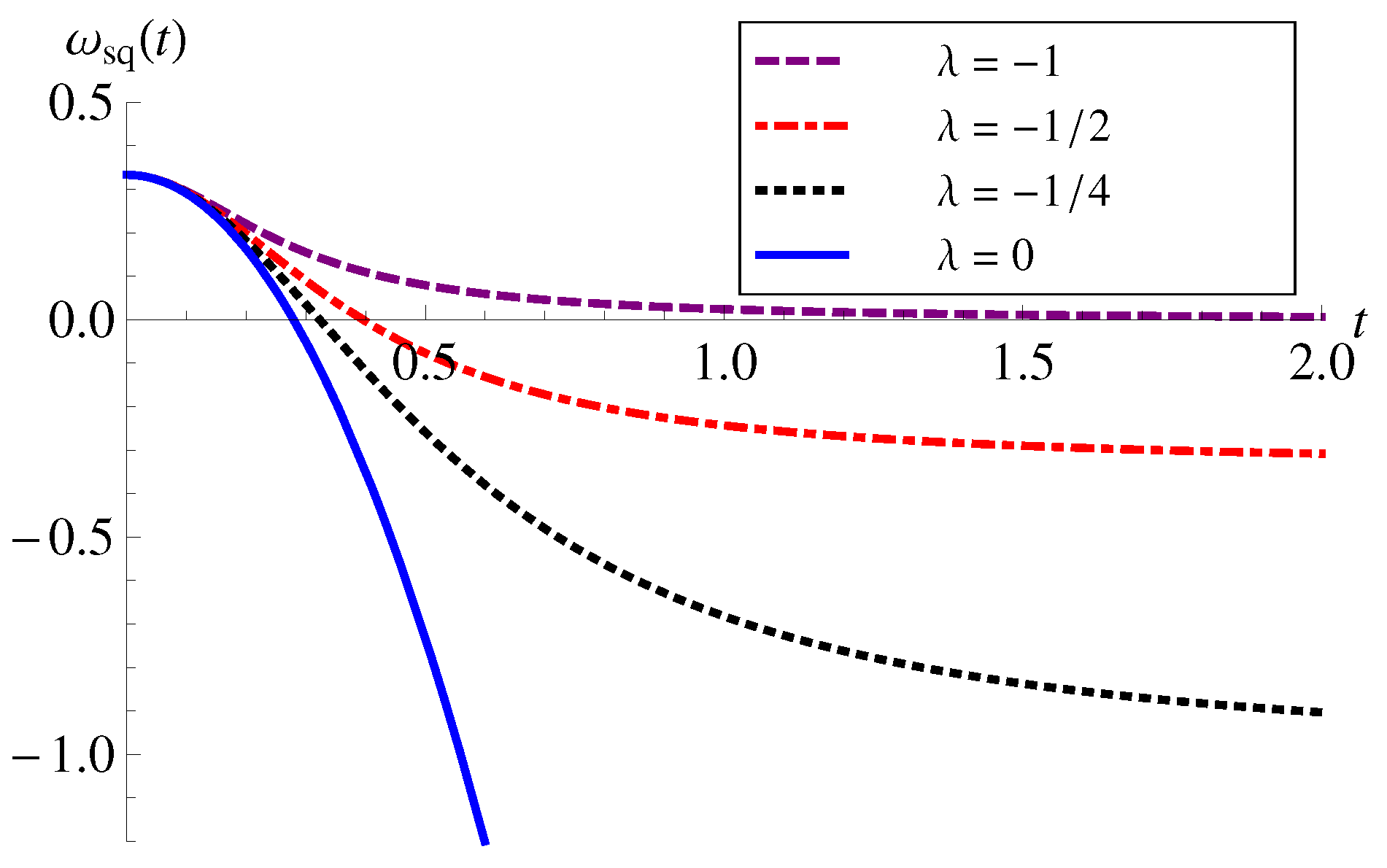
The behavior of SQM is shown in Fig. 1. The EoS parameter, starts from ${\omega }_{sq}=\frac{1}{3}$ (irrespective of any values of n, $B_c$ and $\lambda$) and tends to ${\omega }_{sq}=\frac{1+\lambda }{3\lambda }$, as $t\to \infty$. Hence, the late time behavior of SQM depends solely on the additional terms of $f(R,T)$ gravity. The case $\lambda =0$ corresponds to GR and the EoS describes the transition from ${\omega }_{sq}=\frac{1}{3}$ to phantom matter ${\omega }_{sq}<-1$. In $f(R,T)$ gravity, ${\omega }_{sq}$ does not cross the phantom divide line. It describes the transition from ultra-relativistic radiation to dust (${\omega }_{sq}=0$) for $\lambda =-1$, quintessence (${\omega }_{sq}=-\frac{1}{3}$) for $\lambda =-\frac{1}{2}$, and a cosmological constant (${\omega }_{sq}=-1$) for $\lambda =-\frac{1}{4}$. Though the model describes only a decelerated universe, DE features do not contradict because SQM showing these characteristics is not the net matter.

We mentioned in the introduction that due to the coupling of matter and geometry, some extra terms do appear in the field equations. These terms having $\lambda$ in $\left(24\right)-\left(26\right)$ can be associated with so-called coupled matter. They can be distinguished as ${\rho }_f$ and $p_f$, respectively. Then ${\rho }_f=4\lambda B_c=-p_f$, hence ${\omega }_f=-1$. Therefore these extra terms contribute as a cosmological constant.

3.1. The effective matter

The energy density and the pressure of the effective matter are found to be equal

$${\rho }_{eff}=\frac{1+2n}{{\left(2+n\right)}^2{t}^2}=p_{eff}.$$

(37)

Hence, the effective matter acts as a stiff matter that justifies the decelerated behavior of the model.

4. Model with special law of Hubble parameter

As we have mentioned in the previous section, Agrawal and Pawar [68] over determined the solutions. They considered two assumptions simultaneously to find the exact solutions. However, only one of them is sufficient as we have seen in the previous section. Here, we consider a model with the other assumption the authors considered in their model, i.e., a special law of variation of the Hubble parameter

$$H=k{\left(A^{2}B\right)}^{-\frac{m}{3}},$$

(38)

where $k>0$, $m\ge 0$ are constants. The deceleration parameter, $q=-\frac{a\ddot{a}}{{\dot{a}}^2}=-1-\frac{\dot{H}}{H^2}$, for the above law yields a constant value

$$q=m-1,$$

(39)

which shows that the models with $m<1$ describe an accelerating universe, while the models with $m>1$ correspond to a decelerating universe. Hence, whilst one could obtain decelerating and accelerating models separately, it is not possible to obtain a model with a transition from one to the other.

From (25)–(26), the condition for isotropy of pressure is

$$\frac{\dot{A}}{A}-\frac{\dot{B}}{B}=\frac{\beta }{A^{2}B},$$

(40)

where $\beta$ is the constant of integration. Using (38) in (12) and solving together with (40), one obtains

$$\begin{array}{ccc}\hfill A& =& \left\{\begin{array}{cc}\alpha t^{\frac{1}{m}}exp\left[\frac{\beta mt{\left(kmt\right)}^{-\frac{3}{m}}}{3(m-3)}\right];\hfill & m\ne 3,\hfill \\ \alpha t^{\frac{3k+\beta }{9k}};\hfill & m=3,\hfill \end{array}\right.\hfill \end{array}$$

(41)

$$\begin{array}{ccc}\hfill B& =& \left\{\begin{array}{cc}\alpha t^{\frac{1}{m}}exp\left[-\frac{2\beta mt{\left(kmt\right)}^{-\frac{3}{m}}}{3(m-3)}\right];\hfill & m\ne 3,\hfill \\ \alpha t^{\frac{3k-2\beta }{9k}};\hfill & m=3,\hfill \end{array}\right.\hfill \end{array}$$

(42)

where $\alpha$ is an integration constant. The geometrical behavior of the model remains the same as in GR [71] (see also [12] for detailed discussion).

Case (i) $m=3$

The directional scale factors A and B follow power law expansion in this case which is similar to the model I. Therefore, the geometrical and physical behavior of the model is similar to model I. The energy density and pressure of QM are obtained as

$$\begin{array}{ccc}\hfill {\rho }_q& =& \frac{9k^2-{\beta }^2}{27k^2{t}^2}-(1+4\lambda )B_c,\hfill \end{array}$$

(43)

$$\begin{array}{ccc}\hfill p_q& =& \frac{1}{3}\left[\frac{9k^2-{\beta }^2}{27k^2{t}^2}-(1+4\lambda )B_c\right].\hfill \end{array}$$

(44)

Consequently, the energy density and pressure of SQM become

$$\begin{array}{ccc}\hfill {\rho }_{sq}& =& \frac{9k^2-{\beta }^2}{27k^2{t}^2}-4\lambda B_c,\hfill \end{array}$$

(45)

$$\begin{array}{ccc}\hfill p_{sq}& =& \frac{1}{3}\left[\frac{9k^2-{\beta }^2}{27k^2{t}^2}-(1+\lambda )4B_c\right].\hfill \end{array}$$

(46)

The constraints ${\beta }^2\le 9k^2$ and $\lambda <-\frac{1}{4}$, imply the WEC holds.

The EoS parameter of the matter can be expressed as

$${\omega }_{sq}=\frac{\frac{1}{3}\left[\frac{9k^2-{\beta }^2}{27k^2{t}^2}-4(1+\lambda )B_c\right]}{\frac{9k^2-{\beta }^2}{27k^2{t}^2}-4\lambda B_c}.$$

(47)

The energy density and pressure of the effective fluid are given by

$${\rho }_{eff}=\frac{9k^2-{\beta }^2}{27k^2{t}^2}=p_{eff}.$$

(48)

All of the above mathematical expressions are almost similar to the model I. We observe that, the physical description given for the model I is true for this model also.

Case (ii) $m\ne 3$

The energy density and pressure of QM in this case become

$$\begin{array}{ccc}\hfill {\rho }_q& =& \frac{3}{m^2{t}^2}-\frac{1}{3}{\beta }^2{\left(kmt\right)}^{-\frac{6}{m}}-(1+4\lambda )B_c,\hfill \end{array}$$

(49)

$$\begin{array}{ccc}\hfill p_d& =& \frac{1}{m^2{t}^2}-\frac{1}{9}{\beta }^2{\left(kmt\right)}^{-\frac{6}{m}}-\frac{1}{3}(1+4\lambda )B_c.\hfill \end{array}$$

(50)

Therefore, the energy density and pressure of SQM turn out to be

$$\begin{array}{ccc}\hfill {\rho }_{sq}& =& \frac{3}{m^2{t}^2}-\frac{1}{3}{\beta }^2{\left(kmt\right)}^{-\frac{6}{m}}-4\lambda B_c,\hfill \end{array}$$

(51)

$$\begin{array}{ccc}\hfill p_{sq}& =& \frac{1}{m^2{t}^2}-\frac{1}{9}{\beta }^2{\left(kmt\right)}^{-\frac{6}{m}}-\frac{4}{3}(1+\lambda )B_c.\hfill \end{array}$$

(52)

From (49), we see that for $\lambda >-\frac{1}{4}$, the model violates the WEC at late times, as well as at early times. However, the violation of the WEC at late times can be avoided by the restriction $\lambda \le -\frac{1}{4}$, but it cannot be avoided at early times unless $\beta =0$, in which case the model is isotropic. Hence, an anisotropic model is not physically viable for $m\ne 3$.

In order to satisfy the WEC we must have $\lambda <-\frac{1}{4}$. The EoS parameter of a SQM can be expressed as

$${\omega }_{sq}=\frac{\frac{1}{3}\left[\frac{3}{m^2{t}^2}-\frac{1}{3}{\beta }^2{\left(kmt\right)}^{-\frac{6}{m}}-(1+\lambda )4B_c\right]}{\frac{3}{m^2{t}^2}-\frac{1}{3}{\beta }^2{\left(kmt\right)}^{-\frac{6}{m}}-4\lambda B_c}.$$

(53)

In this model same results are obtained as mentioned as in sect. 3. It is clear that ${\omega }_{sq}$ relies on both the additional terms of $f(R,T)$ gravity and bag constant. However, if $B_c=0$, the model neither depends on the additional terms of $f(R,T)$ nor the bag constant, i.e., $B_c=0$, ${\omega }_{sq}=\frac{1}{3}={\omega }_q$, where ${\omega }_q$ is the $EoS$ of $QM$, hence exhibiting ultra-relativistic radiation. Then, in the absence of the additional terms of $f(R,T)$ gravity, ${\omega }_{sq}=\frac{1}{3}+\frac{4B_c{\left(kmt\right)}^{\frac{6}{m}}}{\beta }$ at $t\to 0$, ${\omega }_{sq}=\frac{1}{3}$, i.e., a semi-realistic model $(\omega \ge 0)$.

4.1. The effective matter

The energy density and pressure of the effective fluid for case $\left(i\right)$ is given by

$${\rho }_{eff}=\frac{9k^2-{\beta }^2}{27k^2{t}^2}=p_{eff},$$

(54)

for $9k^2>{\beta }^2$, i.e., stiff matter. on the other hand, in case $\left(ii\right)$, we have

$${\rho }_{eff}=-\frac{1}{3}{\beta }^2{\left(kmt\right)}^{-\frac{6}{m}},$$

(55)

$$p_{eff}=\frac{1}{3}{\left(kmt\right)}^{\frac{6}{m}}\left(6k\beta {\left(kmt\right)}^{-1+\frac{3}{m}}-{\beta }^2\right).$$

(56)

Then the $EoS$ parameter for positive values of $\beta ,k,m$ is given by

$${\omega }_{eff}=1+\frac{{\left(kmt\right)}^{-1+\frac{3}{m}}}{\beta }.$$

(57)

In this instance, the model shows a transition from ${\omega }_{eff}=1$ to ${\omega }_{eff}\to \infty$ as $t\to \infty$, for $0<m\le 3$, $k,\beta >0$. In this case it exhibits a a transition from stiff matter to a semi-realistic matter $({\omega }_{eff}>0)$.

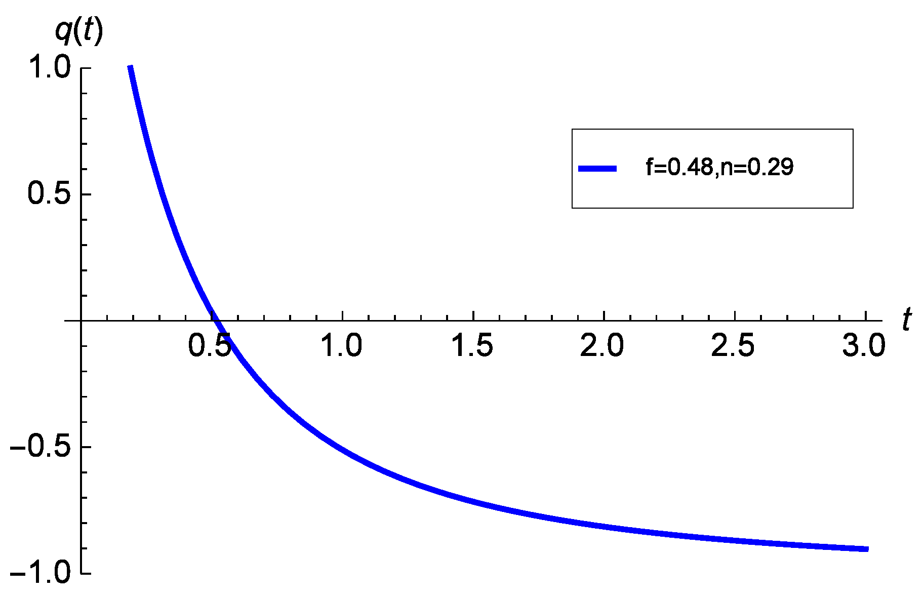
5. Model with Hybrid scale factor

Based on various observational data [1,2], it is evident that the cosmic acceleration of the universe is a recent phenomenon and hence there must be a transition from early deceleration to late time accelerated expansion sometime in the recent past. In view of this phenomenon, in this section, we have used a time varying DP (TVDP) to comprehend the current universe that flips signature from early deceleration to late time acceleration. This means that the deceleration parameter should be positive ($q>0$) early on and at some time, signature flipping occurs, after which $q<0$. Whilst in the previous sections, we have studied models with both deceleration as well as acceleration, the considered models do not exhibit such a change. So in this section we have analysed a hybrid scale factor [72] given by

$$a\left(t\right)=e^{ft}{t}^g,$$

(58)

where $f,g$ are positive constants (we have set a constant equal to unity without loss of generality). Much work has been done in homogeneous and both isotropic and anisotropic space-times (e.g., [73,74,75,76]).

To visualise the transition, we have plotted the deceleration parameter q against time t in the Figure 2.

The energy density and pressure of QM in this model are obtained as

$${\rho }_q=3f^2+\frac{3g^2}{t^2}+\frac{6fg}{t}+\frac{{\beta }^2{t}^{-6g}}{3e^{6ft}}-(1+4\lambda )B_c,$$

(59)

$$p_q=\frac{1}{3}\left[3f^2+\frac{3g^2}{t^2}+\frac{6fg}{t}+\frac{{\beta }^2{t}^{-6g}}{3e^{6ft}}-(1+4\lambda )B_c\right].$$

(60)

Consequently, the energy density and pressure of SQM yields

$${\rho }_{sq}=3f^2+\frac{3g^2}{t^2}+\frac{6fg}{t}+\frac{{\beta }^2{t}^{-6g}}{3e^{6ft}}-4\lambda B_c,$$

(61)

$$p_{sq}=\frac{1}{3}\left[3f^2+\frac{3g^2}{t^2}+\frac{6fg}{t}+\frac{{\beta }^2{t}^{-6g}}{3e^{6ft}}-(1+\lambda )4B_c\right].$$

(62)

The constraints $f>0,0<g<3,\beta >0,\lambda <-\frac{1}{4}$, imply that the WEC holds. The EoS parameter of the matter can be expressed as

$${\omega }_{sq}=\frac{\frac{1}{3}\left[3f^2+\frac{3g^2}{t^2}+\frac{6fg}{t}+\frac{{\beta }^2{t}^{-6g}}{3e^{6ft}}-(1+\lambda )4B_c\right]}{3f^2+\frac{3g^2}{t^2}+\frac{6fg}{t}+\frac{{\beta }^2{t}^{-6g}}{3e^{6ft}}-4\lambda B_c}.$$

(63)

In this model, we have the same results as mentioned in model-II. It is clear that in this case, the model depends on the bag constant $B_c$ and $f(R,T)$ gravity. Yet, when $B_c=0$, the model neither depends on the additional terms of $f(R,T)$ nor the bag constant, i.e., $B_c=0$, ${\omega }_{sq}=\frac{1}{3}={\omega }_q$, where ${\omega }_q$ is the EoS of QM, hence corresponding to ultra-relativistic radiation. For $f>0$, $0<g<0.3$, $B_c=2$, $\beta =2$ and $\lambda =-\frac{1}{4}$, the model evolves from radiation to a cosmological constant, while if $\lambda =-\frac{1}{2}$, the model initially is in a radiation phase, and then later mimics quintessence. Lastly for $\lambda =-1$, the model is only in a radiation phase. We can conclude that for constrained parameters of $f,g,\lambda$, the hybrid scale factor model behaves similarly to model I.

5.1. The model in GR

In GR, i.e., $\lambda =0$, this model solely relies on the bag constant only. Hence, from (62), we get

$${\omega }_{sq}=\frac{\frac{1}{3}\left[3f^2+\frac{3g^2}{t^2}+\frac{6fg}{t}+\frac{{\beta }^2{t}^{-6g}}{3e^{6ft}}-4B_c\right]}{3f^2+\frac{3g^2}{t^2}+\frac{6fg}{t}+\frac{{\beta }^2{t}^{-6g}}{3e^{6ft}}}.$$

(64)

In this model the EoS exhibits a smooth transition from ${\omega }_{sq}=\frac{1}{3}$ (ultra-relativistic radiation) to ${\omega }_{sq}\to -\infty$ (phantom matter). Thus in GR, the EoS describes all kinds of known matter (radiation, dust, quintessence, cosmological constant and phantom matter). This model fits well with observations, including the late-time accelerated expansion of the universe [77,78,79,80,81]. If $-1\le \omega \le -\frac{1}{3}$, then we have quintessence [82,83] and if $\omega <-1$, then we have a phantom model [84,85]. The phantom matter is well supported by observations [86].

6. Conclusions

In this paper, we have studied an LRS bianchi-I space-time in $f(R,T)$ gravity, where $f(R,T)=R+2f\left(T\right)$ with $f\left(T\right)=\lambda T$. We have considered a model with SQM [68], and it is important to mention that the solutions obtained assume an expansion scalar proportional to the shear scalar. This returns a constant value for the deceleration parameter, $q=2$. Hence, the model can describe only the decelerated era of the universe. The metric potentials $A,B$ in [68] are not correct as they can be obtained by means of equations (25)–(26) and (27). The other setback of their model is that the LHS of their field equations are not correct and physically invalid. Since the assumption $(\theta =3H)$ has already been considered by [87,88,89], we can see that the wrong signs do not affect the geometrical parameters. The comparisons of the outcomes in $f(R,T)$ gravity and bag constant has been done to comprehend their roles. It is to be noted that the geometrical parameters of model 1 has been calculated [26], in which ref the physical viability constraints of the model ignored in [68] has been considered.

In the model with $B=A^n$ in $f(R,T)$, we found that it is physically viable for $\lambda <-1/4,n>-\frac{1}{2}$. It is also important to mention that when working with $f(R,T)$ gravity, there are some additional terms appearing on the right hand side of the field equations as compared to GR. Due to the coupling of matter and geometry, those terms can be treated as some additional matter. If this coupling matter is treated as matter, then it is physically viable for $\lambda >0$. They contribute as a cosmological constant.

The overall model depends on both the additional terms of $f(R,T)$ gravity and bag constant $B_c$. Hence if $B_c=0$, the model starts off with ultra-relativistic radiation, hence behaving the same as QM. We can also observe that $B_c$ depends solely on the additional terms $f(R,T)$ gravity. Then for some values of $\lambda$, the model describes a variety of matter including dust, quintessence and the cosmological constant. We can conclude that $f(R,T)$ gravity enables a transition from ultra-relativistic radiation to the cosmological constant. In GR, i.e., $\lambda =0$, the model of course rely on the bag constant only. Again, we can see clearly that the model starts off as radiation and later to all dynamical candidates including phantom. Hence in this case, we can see that the bag constant enables a transition from ultra-relativistic radiation to finally, phantom matter.

In the second model where the assumption $H=k{\left(A^{2}B\right)}^{-m}$, $m,k>0$, has been considered, two cases have been studied. The physical viability of the solutions has also been checked where in case (i) for $\lambda <-\frac{1}{4},9k^2\ge {\beta }^2$ the model is physically viable. In case (ii), all solutions are physically viable for $\lambda <-\frac{1}{4},\beta ,k,m>0$. Then from the deceleration parameter we can chose the accelerating model. For $m=3$, for the constraints mentioned in case (i), again in this instance the model depends both on the additional terms of $f(R,T)$ gravity and the bag constant $B_c$. This case shares the same features as in model 1, i.e., $f(R,T)$ gravity enables a transition from ultra-relativistic radiation to a cosmological constant for some values of $\lambda$. In GR, the model starts off with ultra-relativistic matter and ending in phantom matter. In case (ii), where $m\ne 3$, the model behaves the same as in case (i). Except for $\lambda =0$ (GR), it starts off from ultra-relativistic radiation, and then ends up with a semi-realistic EoS $\omega >0$.

Since the metric potentials are independent of the bag constant or the additional terms of $f(R,T)$ gravity, the effective matter in model 1 will act as stiff matter. Again in case (i), it acts as stiff matter also. Hence in case (ii), it starts from stiff matter to and ends with a semi-realistic EoS, $\omega >0$, for some values of $0<m\le 3$, $\beta ,k>0$.

References

- Riess, A.G.; Filippenko, A.V.; Challis, P.; Clocchiatti, A.; Diercks, A.; Garnavich, P. M.; Gilliland, R. L.; Hogan, C.J.; Jha, A.; Kirshner, R.P.; et al. Observational Evidence from Supernovae for an Accelerating Universe and a Cosmological Constant. Astron. J. 1998, 116, 1009–1038. [Google Scholar] [CrossRef]
- Perlmutter, S.; Aldering, G.; Goldhaber, G.; Knop, R.A.; Nugent, P.; Castro, P.G.; Deustua, S.; Fabbro, S.; Goobar, A.; Groom, D.E.; et al. Measurements of Ω and Λ from 42 High-Redshift Supernovae. Astrophys. J. 1999, 517, 565–586. [Google Scholar] [CrossRef]
- Schmidt, B.P.; Suntzeff, N.B.; Phillips, M.M.; Schommer, R.A.; Clocchiatti, A.; Kirshner, R.P.; Garnavich, P.; Challis, P.; Leibundgut, B.; Spyromilio, J.; et al. The High-Z Supernova Search: Measuring Cosmic Deceleration and Global Curvature of the Universe Using Type Ia Supernovae. Astrophys. J. 1998, 507, 46–63. [Google Scholar] [CrossRef]
- Bamba, K.; Capozziello, S.; Nojiri, S.; Odintsov, S.D. Dark energy cosmology: The equivalent description via different theoretical models and cosmography tests. Astrophys. Space Sci. 2012, 342, 155–228. [Google Scholar] [CrossRef]
- Nojiri, S.; Odintsov, S.D. Unified cosmic history in modified gravity: From F(R) theory to Lorentz non-invariant models. Phys. Rep. 2011, 505, 59–114. [Google Scholar] [CrossRef]
- Zlatev, I.; Wang, L.; Steinhardt, P.J. Quintessence, Cosmic Coincidence, and the Cosmological Constant. Phys. Rev. Lett. 1999, 82, 896. [Google Scholar] [CrossRef]
- Peebles, J.E.; Ratra, B. The cosmological constant and dark energy. Rev. Mod. Phys. 2003, 75, 559. [Google Scholar] [CrossRef]
- Linde, A.D. A new inflationary universe scenario: A possible solution of the horizon, flatness, homogeneity, isotropy and primordial monopole problems. Phys. Lett. B 1982, 108, 389–393. [Google Scholar] [CrossRef]
- Misner, C.W. The Isotropy of the Universe. Astrophys. J. 1968, 151, 431. [Google Scholar] [CrossRef]
- Weinberg, S. Gravitation and Cosmology: Principles and Applications of the General Theory of Relativity, 1st ed.; John Wiley and Sons: New York, NY, USA, 1972. [Google Scholar]
- Harko, T.; Lobo, F.S.N.; Nojiri, S.; Odintsov, S.D. f(R, T) gravity. Phys. Rev. D 2011, 84, 024020. [Google Scholar] [CrossRef]
- Singh, V.; Beesham, A. Plane symmetric model in f(R, T) gravity. Eur. Phys. J. Plus 2020, 135, 319. [Google Scholar] [CrossRef]
- Jamil, M.; Momeni, M.; Raza, M.; Myrzakulov, R. Reconstruction of some cosmological models in f (R, T) cosmology. Eur. Phys. J. C 2012, 72, 1999. [Google Scholar] [CrossRef]
- Shabani, H.; Farhoudi, M. f (R, T) cosmological models in phase space. Phys. Rev. D 2013, 88, 044048. [Google Scholar] [CrossRef]
- Santos, A.F.; Ferst, C.J. Godel-type solution in f (R, T) modified gravity. Mod. Phys. Lett. A 2015, 30, 1550214. [Google Scholar] [CrossRef]
- Alhamzawi, A.; Alhamzawi, R. Gravitational lensing by f (R, T) gravity. Int. J. Mod. Phys. D 35, 1650020 (2016).
- H. Shabani, A. H. H. Shabani, A. H. Ziaie. Eur. Phys. J. C 78, 397 (2018).
- Ordines, T.M.; Carlson, E.D. Limits on f (R, T) gravity from Earth’s atmosphere. Phys. Rev. D 2019, 104052. [Google Scholar] [CrossRef]
- Netterfield, C.B.; et al. A measurement by BOOMERANG of multiple peaks in the angular power spectrum of the cosmic microwave background. Astrophy. J. 2002, 571, 604–614. [Google Scholar] [CrossRef]
- Hinshaw, G.; et al. Nine-year Wilkinson Microwave Anisotropy Probe (WMAP) Observations: Cosmological Parameter Results. Astrophys. J. Supp. Ser. 2013, 19. [Google Scholar] [CrossRef]
- Bennett, C.L.; et al. Nine-year Wilkinson Microwave Anisotropy Probe (WMAP) observations: final maps and results. Astrophy. J. Supp. Ser. 2013, 208(2), 20. [Google Scholar] [CrossRef]
- Planck Collaboration. arXiv:gr-qc/1807.06209.
- Reddy, D.R.K.; Naidu, R.L.; Satyanarayana, B. Kaluza-Klein Cosmological Model in f(R,T) Gravity. Int. J. Theor. Phys. 2012, 51, 3222. [Google Scholar] [CrossRef]
- Ram, S. ; Priyanka. Some Kaluza-Klein cosmological models in f(R, T) gravity theory. Astrophys. Space Sci. 2013, 347, 389–397.
- Sharif, M.F.; Zubair, M. Energy Conditions Constraints and Stability of Power Law Solutions in f(R, T) Gravity. J. Phys. Soc. Jpn. 2013, 82, 014002. [Google Scholar] [CrossRef]
- Shamir, M.F. Bianchi Type I Cosmology in f(R, T) Gravity. J. Exp. Theor. Phys. 2014, 119, 242–250. [Google Scholar] [CrossRef]
- Moraes, P.H.R.S.; Correa, R.A.C.; Ribeiro, G. Evading the non-continuity equation in the f(R, T) cosmology. Eur. Phys. J. C 2018, 78, 192. [Google Scholar] [CrossRef]
- Tiwari, R.K.; Beesham, A. Anisotropic model with decaying cosmological term. Astrophys. Space Sci. 2018, 363, 234. [Google Scholar] [CrossRef]
- Esmaeili, F.M. Dynamics of Bianchi I Universe in Extended Gravity with Scale Factors. J. High Energy Phys. Gravit. Cosmol. 2018, 4, 716–730. [Google Scholar] [CrossRef]
- Itoh, N. Hydrostatic Equilibrium of Hypothetical Quark Stars. Prog. Theor. Phys. 1970, 44, 291–292. [Google Scholar] [CrossRef]
- Bodmer, A.R. Collapsed Nuclei. Phys. Rev. D 1971, 4, 1601–1606. [Google Scholar] [CrossRef]
- Witten, E. Cosmic separation of phases. Phys. Rev. D 1984, 30, 272. [Google Scholar] [CrossRef]
- Mak, M.K.; Harko, T. Quark stars admitting a one-parameter group of conformal motions. Int. J. Mod. Phys. D 2004, 13, 149–156. [Google Scholar] [CrossRef]
- Farhi, E.; Jaffe, R.L. Strange matter. Phys. Rev. D 1984, 30, 2379. [Google Scholar] [CrossRef]
- Alcock, C.; Farhi, E.; Olinto, A. Strange Stars. Astrophys. J. 1986, 310, 261–272. [Google Scholar] [CrossRef]
- Haensel, P.; Zdunik, J.L.; Schaefer, R. Strange quark stars. Astron Astrophys. 1986, 160, 121–128. [Google Scholar]
- Madsen, J. Physics and astrophysics of strange quark matter. In Hadrons in Dense Matter and Hadrosynthesis, Lecture Notes in Physics; Springer: Berlin/Heidelberg, Germany, 1999; Volume 516, pp. 162–203. [Google Scholar]
- Drake, J.J.; Marshall, H.L.; Dreizler, S.; Freeman, P.E.; Fruscione, A.; Juda, M.; Kashyap, V.; Nicastro, F.; Pease, D.O.; Wargelin, B.J.; et al. Is RX J185635-375 a Quark Star? Astrophys. J. 2002, 572, 996–1001. [Google Scholar] [CrossRef]
- Weber, F. Strange Quark Matter and Compact Stars. Prog. Part. Nucl. Phys. 2005, 54, 193–288. [Google Scholar] [CrossRef]
- Aktas, C.; Yilmaz, I. Is the universe homogeneous and isotropic in the time when quark-gluon plasma exists? Gen. Relativ. Grav. 2011, 43, 1577–1591. [Google Scholar] [CrossRef]
- Berger, M.S. ; Jaffe. R.L.Quark exchange in nuclei and the European Muon Collaboration effect. Phys. Rev. C 1987, 35, 1. [Google Scholar]
- Peng, G.X.; Li, A.; Lombardo, U. Deconfinement phase transition in hybrid neutron stars from the Brueckner theory with three-body forces and a quark model with chiral mass scaling. Phys. Rev. C 2008, 62, 025801. [Google Scholar] [CrossRef]
- Alford, M.K.; Reddy, S. Compact stars with color superconducting quark matter. Phys. Rev. D 2003, 67, 7. [Google Scholar] [CrossRef]
- Weissenborn. S.; et al.Quark matter in massive compact stars. Astrophys. J. Lett. 2011, 740, 1.
- Sinha, B. The microsecond old universe relics of qcd phase transition. Int. J. Mod. Phys. A 2014, 29, 23. [Google Scholar] [CrossRef]
- Xia, C.J.; et al. Properties of strange quark matter objects with two types of surface treatments. Phys. Rev. D 2016, 8, 085025. [Google Scholar] [CrossRef]
- Geng, J.J.; Huang, Y.F. ; Lu. T. Coalescence of Strange-quark Planets with Strange Stars: A New Kind of Source for Gravitational Wave Bursts. Astrophys. J. 2015, 804, 1, p.
- Fraga, E.S. ; Kurkela, A Vuorinen. A. Interacting quark matter equation of state for compact stars. Astrophys. J. Lett. 2014, 781, 2, p.L25.
- Boeckel, T.; Schaffner-Bielich, J. A. little inflation in the early universe at the QCD phase transition. Phys. Rev. Lett. 2010, 105, 041301. [Google Scholar] [CrossRef]
- Yilmaz, I.; Aktas, C. Space-time geometry of quark and strange quark matter. Chin. J. Astron. Astrophys. 2007, 6, 757. [Google Scholar] [CrossRef]
- Khadekar, G. S.; Rupali, W. Geometry of quark and strange quark matter in higher dimensional general relativity. Int. J. Theor. Phys. 2012, 51, 1408–1415. [Google Scholar] [CrossRef]
- Rao, V.U.M.; Neelima, D. Cosmological models with strange quark matter attached to string cloud in GR and Brans-Dicke theory of gravitation. Euro. Phys. J. Plus. 2014, 129, 1–7. [Google Scholar] [CrossRef]
- Gholizade, H. ; ltaibayeva. A. Thermodynamics and geometry of strange quark matter. Int. J. Theor. Phys. 2015, 54, 2107–2118. [Google Scholar]
- Rao, V.U.M.; Neelima, D. Axially symmetric space-time with strange Quark matter attached to string cloud in self creation theory and general relativity. Inter. J. Theor. Phys. 2013, 52, 354–361. [Google Scholar] [CrossRef]
- Khadekar, G.S.; Shelote, R. Higher dimensional cosmological model with quark and strange quark matter. Int. J. Theor. Phys. 2012, 51(5), 1442–1447. [Google Scholar] [CrossRef]
- Aktas, C.; Yilmaz, İ. Magnetized quark and strange quark matter in the spherical symmetric space–time admitting conformal motion. Gen. Rel. Grav. 2007, 39:849–862.
- Barrow,J. D.; et al. Cosmology with inhomogeneous magnetic fields. Phys. Rep. 2007, 449(6), 131–171.
- I. Yılmaz, I. I. Yılmaz, I.; Baysal, Hü, Aktaş, C. Quark and strange quark matter in f (R) gravity for Bianchi type I and V space-times. Gen. Rel. Grav. 2012, 44, 2313-2328.
- Adhav, K. S.; Bansod, A.S.; Munde, S. L. Kantowski-Sachs Cosmological model with quark and strange quark matter in f (R) theory of gravity. Open Phys. 2015, 1. [Google Scholar]
- Santhi, M. V.; Chinnappalanaidu, T. Strange quark matter cosmological models attached to string cloud in f (R) theory of gravity. Ind. J. Phys. 2022, 96(3), 953–962. [Google Scholar] [CrossRef]
- Rahaman, F.; et al. Quark matter as dark matter in modeling galactic halo. Phys. Lett. B 714(2-5), 131-135.
- Yavuz, I.; Yilmaz, I. ; Baysal, Hü. Strange quark matter attached to the string cloud in the spherical symmetric space–time admitting conformal motion. Int. J. Mod. Phys. D 2005, 14(08), 1365-1372.
- Mahanta, K. L.; et al. String cloud with quark matter in self-creation cosmology. Int. J. Theor. Phys. 2012, 51, 1538–1544. [Google Scholar] [CrossRef]
- Yilmaz, İ. Domain wall solutions in the nonstatic and stationary Gödel universes with a cosmological constant. Phys. Rev. D 2005, 71(10), 103503. [Google Scholar] [CrossRef]
- Yilmaz, İ.; Baysal, H. Rigidly rotating strange quark stars. Int. J. Mod. Phys. D 2005, 14(03n04), 697–705. [Google Scholar] [CrossRef]
- Yilmaz, İ. String cloud and domain walls with quark matter in 5-D Kaluza–Klein cosmological model. Gen. Rev. Grav. 2006, 38, 1397–1406. [Google Scholar] [CrossRef]
- Adhav, K. S.; Nimkar, A. S.; Dawande, M. V. String Cloud and Domain Walls with Quark Matter in n-Dimensional Kaluza-Klein Cosmological Model. Int. J. Theor. Phys. 2008, 47, 2002–2010. [Google Scholar] [CrossRef]
- Agrawal, P.K.; Pawar, D.D. Plane Symmetric Cosmological Model with Quark and Strange Quark Matter in f (R, T) Theory of Gravity. J. Astrophys. Astron. 2017, 38, 2. [Google Scholar] [CrossRef]
- Berman, M.S. A special law of variation for Hubble’s parameter. Nuovo Cimento B 1983, 74, 182-186.
- Sahoo, P. K. ; B. Mishra, B.; Reddy. G. C. Axially symmetric cosmological model in f (R, T) gravity. Eur. Phys. J. Plus 2014, 129, 1-8.
- Singh, V.; Beesham, A. LRS Bianchi I model with constant deceleration parameter. Gen. Relativ. Grav. 2019, 51(12), 166. [Google Scholar] [CrossRef]
- Akarsu, Ö.; et al. Cosmology with hybrid expansion law: scalar field reconstruction of cosmic history and observational constraints. J. Cosmol. Astropart. Phys.
- Nagpal, R.; Singh, J.K.; and Aygün, S. FLRW cosmological models with quark and strange quark matters in f (R, T) f(R,T) gravity. Astrophys. Space Sci. 2018, 363, 1–12. [Google Scholar] [CrossRef]
- Singh, V.; Beesham, A. LRS Bianchi I model with strange quark matter and Λ(t)in f (R, T) gravity. New Astronomy 2021, 89, 101634. [Google Scholar] [CrossRef]
- Bishi, B.K.; Beesham, A.; and Mahanta, K.L. Domain Walls and Quark Matter Cosmological Models in f (R, T)= R+ α R 2+ λ T f (R, T)= R+ α R 2+ λ T Gravity. J. Sci. Technol. Trans. A: Sci.
- Vijaya S, M.; Chinnappalanaidu, T. Bianchi type strange quark cosmological models in a modified theory of gravity. Afrika Matematika 2022, 33(4), 1–33. [Google Scholar] [CrossRef]
- Komatsu, E.; et al. Five-year Wilkinson microwave anisotropy probe (WMAP) observations: Cosmological interpretation. Astrophys. J. Suppl. 2009, arXiv:astro-ph/0803.0547(180), 330–376. [Google Scholar] [CrossRef]
- Ade, P. A. R.; et al. . Planck 2015 results XX. Constraints on inflation. Astron. Astrophys. 2016, arXiv:astro-ph/1502.02114(594), astro–ph/150202114. [Google Scholar]
- Bean, R.; Hansen, S. H.; and Melchiorri, A. Early-universe constraints on a Primordial Scaling Field, arXiv preprint astro-ph/0104162.
- Hannestad, S.; Mörtsell, E. Probing the dark side: Constraints on the dark energy equation of state from CMB, large scale structure, and type Ia supernovae. Phys. Rev. D 2002, 2002(16), 063508. [Google Scholar] [CrossRef]
- Melchiorri, A.; et al. The state of the dark energy equation of state. Phys. Rev. D 2003, (68), 043509. [Google Scholar] [CrossRef]
- Chiba, T. Quintessence, the gravitational constant, and gravity. Phys. Rev. D 1999, (60), 083508. [Google Scholar] [CrossRef]
- Amendola, L. Coupled quintessence. Phys. Rev. D 2000, (62), 043511. [Google Scholar] [CrossRef]
- Caldwell, R. R.; et al. Phantom energy dark energy with causes a cosmic doomsday. Phys. Rev. Lett. 2003, (91), 071301. [Google Scholar] [CrossRef]
- Martin, J. Quintessence: a mini-review. Mod. Phys. Lett. A 2008, (23), 1252–1265. [Google Scholar] [CrossRef]
- Tonry, J. L.; et al. Cosmological results from high-z supernovae. Astrophys. J. 2003, (512), 1. [Google Scholar] [CrossRef]
- Mahanta, K.L. Bulk viscous cosmological models in f(R,T) theory of gravity. Astrophys. Space Sci. 2014, 353, 683. [Google Scholar] [CrossRef]
- Jokweni, S.; Singh, V.; Beesham, A. LRS Bianchi I Model with Bulk Viscosity in Gravity. Gravitation and Cosmology 2021, 27(2), 169–177. [Google Scholar] [CrossRef]
- Shamir, M.F. Locally Rotationally Symmetric Bianchi Type I Cosmology in f(R,T) Gravity. Eur. Phys. J. C 2015, 75, 354. [Google Scholar] [CrossRef]