Submitted:
23 August 2023
Posted:
24 August 2023
You are already at the latest version
Abstract
The focus of the current research indicates a new Bianchi type-V anisotropic, homogeneous astrophysical model with modified theory of f(R, T) gravity and Λ(t), time-dependent cosmological constant. The significant effect of the model is that the field equations solutions find using a time-dependent quadratic deceleration parameter. We observed anisotropy parameter remains constant both in the belated universe and early universe. The deportment of the equation of state (EOS) parameter, pressure, and energy density, cosmological constant and other parameters are also discussed. This cosmological model indicated the possibility of an accelerating universe with negative pressure, such as a universe dominated by dark energy. Om(z) diagnostic test suggested that the universe starts with quintessence nature and ends as a phantom model. Also, energy conditions of this model are represented here to ensure the model is physically reasonable and based on observations.
Keywords:
Bianchi type-V
; f(R
; T) gravity
; Time-dependent Cosmological constant
; Deceleration Parameter
; Big Rip
1. Introduction
A cosmological model is a theoretical blueprint for the cosmic order at enormous scales. It has its foundation in the most fundamental ideas of physics and the findings of astrophysicists and cosmologists. The most recognized cosmological theory is the Lambda Cold Dark Matter (CDM) model that states that dark matter and black energy exist alongside regular stuff in a flat universe. The most recent Planck collaboration findings show that around of the components of the cosmos are mysterious. According to General Relativity, the observed cosmic acceleration can be traced to a strange and highly pressurized region of the cosmos that makes up roughly of the universe’s total energy [1,2]. However, gravitational theories, at present, are facing a major theoretical challenge as a result of recent observational findings regarding the Universe’s acceleration in late epoch and the possibility of dark energy [3,4]. One option to explain the data is to assume that the field of gravity is defined by a more universal action and Einstein’s general relativity gravity model fails at very large scales. Perhaps the most amazing insight in modern cosmology was this one. Any arbitrary function can be used to replace the Einstein-Hilbert action’s Ricci scalar R in general relativity is represented as to produce negative pressure and acceleration throughout the cosmos. Complex solutions of the non-linear Ricci scalar have produced diametrically opposed hypotheses. In 2011, Harko and colleagues presented three cosmological explanations for [5,6] as:
Abstract function incorporates both the Ricci scalar R and the trace of the energy-momentum tensor T as indicated by reference [14]. In recent time, scholars have shown a growing fascination with the gravity theory. This theory extends the conventional Einstein-Hilbert action by introducing the concept of which essentially entails a function of the Ricci scalar R. Including the quantity which is necessary at small curvatures, the cosmic acceleration may be explained [7,8]. Owing to significant models of in cosmological scenarios, the hypothesis appears to be the most suited. There have been a few workable gravity models put forth that support combining inflation in the beginning and acceleration towards the end [9]. Feasible gravity models also offer potential solutions to the challenges associated with dark matter. This gravitational framework permits the formulation of a cosmological model devoid of any supplementary singularities which includes inflation in the early cosmos [10,11]. Also, , , , and so on modified gravity theories are now examined in the cosmological model which determines dark energy dominated the universe. A novel type of observational study indicates that approximately is made up of dark energy throughout the universe leads to the expansion which accelerates the universe. To account for this accelerated expansion, scientists have put forward a hypothesis involving a dynamic field within dark energy known as quintessence. Quintessence is described as a scalar field that evolves over time accompanied by a varying equation of state [12,13].
The cosmological model Bianchi type-V is a mathematical representation, an indication of the immense structure and growth of the universe, consisting of both homogeneous and anisotropic, meaning its properties vary in different directions. Specifically, the model proposes that the universe exhibits rotational symmetry around a single axis, with its properties being the same in all directions perpendicular to the axis but differing along the axis itself. The dynamics of this model are governed by the equations of general relativity, which relate the geometry of spacetime to the apportionment of energy and matter within it. The potential of cosmic acceleration, which implies that the universe’s expansion speeds up over time and is thought to be fueled by dark energy, is a key component of the model, Bianchi type-V [15,16].
This paper delves into an examination of a spatially homogeneous and anisotropic Bianchi Type V universe in gravity. The cosmological constant is dynamic over time, and the deceleration parameter is derived by , in which a constant. In Section 2, focusing on the functional form , and considering as , where is a constant that may not necessarily be positive, we establish the fundamental field equations for this model. Finally, the Bianchi type V field equations’ solutions along with expression for various parameter of cosmological importance are shown here. In Section 3, the evolutions of a few significant cosmological parameters are examined, and the geometrical and physical characteristics are described. Then graphical representation and explanations of cosmological parameters are shown for various values of n in section 4. In Section 5, the model’s singularity and removal method are briefly addressed. In section 6, the diagnostic slope with universe behavior is explained, in section 7, an explanation of energy conditions are presented. Finally, in section 8, wrapping up our discussions and conclusions of this model.
2. Field Equations of the Modified Gravity
Harko et al. with his colleagues developed Hilbert-Einstein variational principle depend on gravity field equations [5]. The characteristics of this type of gravity might be stated as
The equations can be obtained by considering a specified form for gravity, denoting , Lagrangian density for matter, R, Ricci scalar, and as trace of . These quantities are interconnected, and the function relies entirely on the metric components . Assuming , and considering that S possesses a distinct action, the formulation process of the equations unfolds as follows:
where refers the derivative that covariates.
Our goal is to choose a functional form of modified gravity that allows us to reduce the field equations in general relativity (GR) by substituting appropriate model parameters. A frequently employed option is , characterized by and . However, we opt to introduce a cosmological constant into the function, rendering it as , in this expression stands as coupling constant that remains independent of time. For that functional choice, the modified theory’s field equation of gravity is expressed as
it is also written as
where the realistic time-dependent cosmological constant is .
When the properties of dark energy exhibit anisotropic characteristics, the computation of its energy-momentum tensor becomes:
The pressure along the three axes is given by , , and correspondingly, whereas denotes fluid’s energy density. EOS parameter is expressed as , where , , and represent the components along three axes. The departure from isotropy is recorded if , with denoting the deviation along axes from . Keep in mind that neither the nor the constants or cosmic time functions.
We explore the influence of cosmic anisotropy by developing a model in the presence of gravity for the Bianchi Type V line element. To introduce anisotropy, we incorporate an anisotropic source that deviates from y and z axes, potentially resembling the presence of cosmic strings, which contributes to an anisotropic directional pressure. Our investigation aims are to understand the impact of the coupling constant on shaping amid cosmic evolution.
2.1. Metric and Field Equations
The form of the cosmological model being considered is that of Bianchi type-V line element is represented as
Both A and B, the metric’s primary scale factors, are determined entirely by the passage of cosmic time. The -plane is associated with a symmetric axis, and the symmetry plane is located along the Z-axis. For the energy-momentum tensor, we obtain eq. as follows:
By using we find the Bianchi type-V metric field equations are
where subscript 1 represents derivative with respect to t.
2.2. Various parameters of cosmological importance
When attempting to solve the previously mentioned equations , it is essential to take into account the following physical parameters as:
An expression for the scale factor and volume V is
H represents the average Hubble parameter as
The following examples illustrate how to provide the Hubble parameters in the three axes, accordingly:
, the scalar describing the rate of expansion, is defined as
and shear scalar is
In this equation, , (where ) is a representation of the directed Hubble parameters. The anisotropy parameter takes the form:
The cosmos expands isotropically when . Additionally, if , , and every anisotropic model of the universe with a energy-momentum tensor along diagonal moves closer to isotropy. Five unknowns (,), three separate equations, and three independent formulae, for solving the set of equations further linkages between the variables are required. The second degree’s time-varying deceleration parameter [19] was investigated mathematically to ascertain the precise field solutions as
n is a constant that is never 0 and is always greater than zero. In most cases, the deceleration parameter is determined by
In the accelerating state of the universe, , strong exponential state when and exhibits a deceleration to acceleration transition phase in the era at . Using and we get
The Hubble parameter H has been demonstrated to indefinite for , , and . And it is always positive for both and as . In this model, we consider .
The scale factor is found by integrating as well as ,
The equation indicates that at the moment , this model enters an initial singular state characterized by . This is followed by a phase of divergence at , at , culminating in a conclusion . The deceleration parameter is equal to both the start and the end of the universe is , and this remains constant. The scale factor s, which Capozziello et al. define in terms concerning the redshift z [20] as
The relation between redshift and cosmic time by using the equation and as follows
Substitute equation in we get
We consider the range of redshift in the model and graphs can be used to condense the earlier findings by selecting n as a constant.
2.3. The Field equations’ cosmological solutions
Physical fact suggests that , we arrived at the relationship shown by
where is a positive constant. Using , and the scale factor A and B can be represented in the subsequent way
and from we have
Since A depends on , therefore, the metric coefficients are expanding at varied rates. Finally, we can write the line element with values of A and B as follows.
The model is represented by the equation in gravity including important kinematical together with physical characteristics that are crucial for examining the cosmological model’s physics.
3. Geometrical and Physical Properties of the Bianchi type V Model
For this model, we now explain some geometrical and mathematical insights of cosmological parameters, differentiating eq. and with respect to time (t). Where, the axis-dependent Hubble parameter is
The Hubble parameters in different directions are linked to varying rates of expansion, which were incredibly high at the beginning of the universe and have since decreased continuously with time. This indicates that the universe was highly uneven in its early stages and gradually became more uniform over time. The scalar expansion is determined by this process, such as
The above expression indicates that has an infinite value at the starting point , and it diverges two points at and . Which indicating universe undergoes a period of extremely rapid expansion in its early stages. The equation for the shear scalar is also provided as follows
Anisotropy parameter can be represented by:
The anisotropy parameter of the Universe remains constant during both early and late times, indicating that the Universe maintains its anisotropic nature throughout its evolution, except for the case when and in which the Universe becomes isotropic at when .
By applying a mathematical constraint where the skewness parameter (), is directly proportional to the EOS parameter (), we attain . To find mathematical expression for physical parameters and , we use equations . Now subtracting equation from we get
and subtracting equation from we get
From equation and we get
Using equation and we get
By utilizing the equation , we can derive the formula for pressure p as
and effective time-dependent cosmological constant
Using in equation and we get the EOS parameter, pressure, equation of energy density, and time-variant cosmological parameter as follows
4. Graphical representations of Cosmological Parameter
Throughtout this paper it has been demonstrated a novel equation governing the second-order time deceleration parameter (q). Our proposed equation combines elements from the model introduced by Akarsu and Tekin (2012), characterized by a linear decrease in q in the first order with a negative gradient, and the models by Berman (1983) and Gomide and Berman (1988), where q remains unchanged. In this model the cosmos is periodic and at undergoes a big-rip before retreating to , its original state. For the perceived kinematics of the universe the appropriate value of n is . But, in this paper, we consider We consider three distinct scenarios: i) when n is less than , ) when n equals , and ) when n is greater than and examine the behavior of the model towards universe.
In Figure 1, for the case , the initial deceleration parameter is . Subsequently, the universe shifts into a decelerating phase during the time interval . In the instance of , the initial deceleration parameter is . It then transitions into an accelerating phase within the time range . Moreover, a distinct phase of rapid exponential expansion is observed during , followed by a decelerated expansion phase at . The commencement of accelerating expansion phase at , with the deceleration parameter exhibiting a value of . Both of these values align well with observations as reported in [24]. Throughout the interval , the deceleration parameter spans the range . Drawing on observational findings, at the present cosmic time (corresponding to the present moment), the deceleration parameter possesses a value of . In the situation where , the initial deceleration parameter is notably high at , leading to a phase of decelerated expansion. Subsequently, the universe transitions into an accelerating phase during the period .
Figure 2: Deceleration parameter with redshift z shows that for and the universe start initially at with and accordingly and then enters transition phase from accelerated to deccelerated expansion with a Big Bang at . For the universe undergoes an accelerated expansion than enters a Big Rip stage at , after that deccelerated expansion continues at .
In Figure 3, at , the Big Rip moment, as well as at initial and final phase of the universe, Hubble parameter diverges for . It shows cyclic behavior. The universe is decelerated expansion for and steady-state expansion at .
Figure 4 reveals that for scale factor enters a transition phase at then behaves as stedy-state, for , this model experiences an initial singularity at time with a value of , followed by a divergent phase at and ultimately ends at , in which at Big Rip occurs . This demonstrates a cyclical behavior in the model. Finally, shows that starting with at gives positive value which determines the universe expansion.
From Figure 5, cosmological constant with respect to time, shows that for , is positive with periodic behavior, which diverges at and starting with an initial Big Bang. For , enters into a Big Bang initially and then enters a transition phase to diverging phase at with decelerated expansion and finally returns the initial stage at . For , the is always negative that predicts a negative energy density and pressure, which might cause the cosmos to contract or experience a big crunch.
Figure 6: shows the relationship between energy density and cosmic time t, showing that energy density is positive at in and takes a Big Rip at . However, when , we observe that energy density diverges at and reaches a Big Rip at with negative value, and when , we notice that the positive energy condition is violated.
Figure 7, represents pressure concerning time t. We see that for pressure diverges at with a positive value and diverges at with negative pressure. value shows, pressure began with a low value and Big Bang then at enters a Big Rip stage with positive pressure and finally returns to the initial Big Bang stage at . It suggests the universe is matter dominated. For , negative pressure permeates the entire universe.
Figure 8, represents the EOS parameter concerning time t. We see that the EOS parameter started with an accelerated expansion to a diverging stage at then it undergoes an accelerated expansion at . shows periodic behavior as well as at the time , and enters Big Rip phase, where diverges. And , , representing energy density is constant and the fluid’s pressure is negligible. Before dark energy takes over, the early cosmos is dominated by dust or matter.
5. Singularity
We have time-based singularity and spatial singularity in General Relativity. In Bianchi type V line element we find time-based singularity where we can use the Raychaudhuri equation to remove singularity [21]. These theorems provide powerful revelations about the structure and behavior of spacetime and have expressive ramifications for the study of black holes and the early universe. The form of the Raychaudhuri equation is determined by the scalar expansion , and it is possible to express it straightforwardly as given below [22]
By using eq. and we have
Introducing deceleration parameter q in eq. we find the form of this equation as follows
If , we have , where the behavior of the expansion scalar and its derivative depends on the behavior of the other variables in the equation. If any of the variables have a vertical tangent line at , the derivative could approach infinity, but it still would not be accurate to say that the derivative is equal to infinity. However, the singularity depends on the sign of . The general requirement of the GR singularity theorems can be used to investigate this, where , indicates singular models. Conversely, non-singular models are identified by . As such at , conclusion that the suggested cosmological model is non-singular as ; where and the cosmological model is singular at . The described model is classified as a Big Rip, where there exists a specific point in time where the Universe begins to gradually decelerate until it eventually reaches its original state.
6. Diagnostic
To apply the diagnostic test to the Bianchi type V line element with the concerning parameter, it is necessary to determine the value using the following equation with redshift variable:
The equation is derived from the Friedmann equation and relates the matter density to the Hubble parameter and gravitational constant G, which are both functions of the redshift. The function can distinguish between alternative dark energy and CDM models. The utilization of test is beneficial in General Relativity to examine the characteristics of dark energy in cosmology. When employed to analyze the Bianchi type V line element, the diagnostic can offer insights into the universe’s evolution and the nature of dark energy [23].
Equation has an alternative form in terms of as:
By examining the function slope, it is possible to assess the dynamic characteristics of dark energy models. A quintessence properties is indicated by a positive diagnostic slope in dark energy model , whereas a phantom nature is indicated by a negative slope. Notably, the slope of the diagnostic tool is unaffected by redshift when ( is utilized in the dark energy model.
From Figure , function is undefined at , it is unable to determine the present-day matter density parameter. Also at the beginning at , the slope is increasing it presents a dark energy model whose nature is called "quintessence" . Later the slope gradually decreases to a constant slope as which refers to a specific type of cosmological model known as the "phantom" model, therefore, dark energy serves as the driving force behind the acceleration that expands the universe.
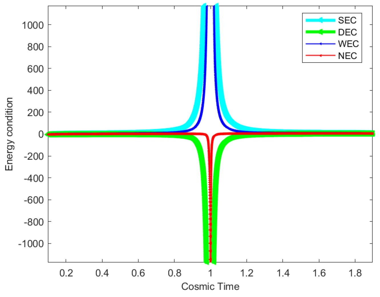
7. Energy conditions for Bianchi type V model
Energy conditions are described with respect to energy density of the matter and its pressure which are the key determinants of spacetime curvature as along with the gravitational behavior. Four basic Weak Energy Conditions (WEC), Null Energy Condition (NEC), Dominant Energy Condition (DEC), and Strong Energy Condition (SEC) are given by
From Figure 10, it can be inferred that the non-negativity conditions are met by the WEC and SEC, whereas the NEC and DEC are not upheld.
8. Conclusions
Throughout this paper, it has been analyzed a Bianchi-type V universe that is both anisotropic and spatially uniform. The universe features a cosmological constant that changes over time and follows a quadratic equation of state in gravity where for the constant . This model, therefore, use quadratic deceleration parameter varying with time. Finally it has been obtained that
- Anisotropy parameter of the Universe remains constant during both early and late times, indicating that the Universe maintains its anisotropic nature throughout its evolution, except for the case when and in which the Universe becomes isotropic at when .
- Larger value of n as decelertion parameter shows that the universe is undergoes anacelerated expansion, but for and this model shows universe deccelerated expansion.
- The nominated cosmological model for is non-singular and singular for . The model is classified as a Big Rip, where the universe gradually decelerates until reaching its original state.
- Initially, the slope of increases, indicating a dark energy model with a "quintessence" nature and as the redshift increases, the slope gradually decreases indicating a dark energy model of the "phantom" type.
- It has been presented graphically and analytically with energy conditions that WEC and SEC hold throughout the considered cosmic time, satisfying the non-negativity conditions. However, NEC and DEC are violated at certain cosmic time. This suggests with a negative pressure component the probability of a universe that accelerates, potentially indicating the universe dominated by dark energy.
By taking into account the model , the more generic solutions to the field equation has also been investigated. Additionally, in order to study the solutions in this situation, no typical assumptions have been made like deceleration parameter or Hubble parameter. For this model, a second-order deceleration parameter has been analyzed in particular. The law that has been presented contains several applications in cosmology not only in the setting of general relativity, but also in cosmology as well as in generalized gravity theories like the , or . Even though the model is straightforward, it can highlight some aspects of the universe’s evolutionary history.
Acknowledgments
The authors appreciate the support received from the “Bose Center for Advanced Study and Research in Natural Sciences”
References
- Mahanta CR, Deka S, Das MP. Bianchi Type V Universe with Time Varying Cosmological Constant and Quadratic Equation of State in f(R,T) Theory of Gravity. East European Journal of Physics 2023, 2, 44–52.
- Pons, J. , and Talavera, P. On cosmological expansion and local physics. General Relativity and Gravitation 2021, 53, 105. [Google Scholar] [CrossRef]
- Amendola L, Tsujikawa S. Dark energy: theory and observations. Cambridge University Press 2010.
- Gawiser, E.; Silk, J. The cosmic microwave background radiation. Physics Reports 2000, 333, 245–267. [Google Scholar] [CrossRef]
- Harko, T. , Lobo, F. S., Nojiri, S., and Odintsov, S. D. f(R,T) gravity. PhysicalReviewD. 2011, 84, 024020. [Google Scholar]
- Pradhan, A. , Goswami, G., and Beesham, A. Reconstruction of an observationally constrained f(R,T) gravity model. arXiv 2023, arXiv:2304.11616. [Google Scholar]
- S. Nojiri, S.D. Odintsov, Problems of modern theoretical physics, a volume in honour of prof. Buchbinder, I.L. in the occasion of his 60th birthday (TSPU Publishing, Tomsk), pp. 266–285.
- Shamir, MF. Locally rotationally symmetric Bianchi type I cosmology in f(R,T) gravity. The European Physical Journal C 2015, 75, 354. [Google Scholar] [CrossRef]
- Capozziello, S. , Farooq, O., Luongo, O., and Ratra, B. Cosmographic bounds on the cosmological deceleration-acceleration transition redshift in f(R) gravity. Physical Review D 2014, 90, 044016. [Google Scholar] [CrossRef]
- Bakry, M. A. , and Shafeek, A. T. The periodic universe with varying deceleration parameter of the second degree. Astrophysics and Space Science 2019, 364, 135. [Google Scholar] [CrossRef]
- Guth, A. H. , and Steinhardt, P. J. The inflationary universe. Scientific American 1984, 250, 116–129. [Google Scholar] [CrossRef]
- Caldwell, R. , and Linder, E. V. Limits of quintessence. Physicalreviewletters 2005, 95, 141301. [Google Scholar]
- Zhang, J. , Zhang, X., and Liu, H. Agegraphic dark energy as a quintessence. The European Physical Journal C 2008, 54, 303–309. [Google Scholar] [CrossRef]
- Alvarenga FG, Houndjo MJ, Monwanou AV, Orou JB. Testing some f(R,T) gravity models from energy conditions. arXiv 2012, arXiv:1205.4678.
- Ahmed N, Pradhan A. Bianchi type-V cosmology in f(R,T) gravity with Λ(T). International Journal of Theoretical Physics 2014, 53, 289–306. [CrossRef]
- Singh T, Chaubey R. Bianchi Type-V universe with a viscous fluid and Λ-term. Pramana 2007, 68, 721–734. [CrossRef]
- Devi, L. A. , Singh, S. S., and Kumrah, L. A new class of interacting anisotropic cosmological models with time varying quadratic deceleration parameter. Indian Journal of Physics 2022, 1–9. [Google Scholar]
- Bakry, M. , Moatimid, G., and Shafeek, A. Cosmological models generated by utilizing a varying polynomial deceleration parameter. Indian Journal of Physics 2022, 1–18. [Google Scholar]
- Bakry, M. A. , and Shafeek, A. T. The periodic universe with varying deceleration parameters of the second degree. Astrophysics and Space Science 2019, 364, 135. [Google Scholar] [CrossRef]
- Capozziello, S. , Farooq, O., Luongo, O., and Ratra, B. Cosmographic bounds on the cosmological deceleration-acceleration transition redshift in f(R) gravity. Physical Review D 2014, 90, 044016. [Google Scholar] [CrossRef]
- Wanas, M. , Kamal, M. M., and Dabash, T. F. Initial singularity and pure geometric field theories. The European Physical Journal Plus 2018, 133, 1–13. [Google Scholar] [CrossRef]
- Horwitz, L. P. , Namboothiri, V. S., Varma K, G., Yahalom, A., Strauss, Y., and Levitan, J. Raychaudhuri equation, geometrical flows and geometrical entropy. Symmetry 2021, 13, 957. [Google Scholar] [CrossRef]
- Liddle, A. R. , and Lyth, D. H. Cosmologicalinflationandlarge-scalestructure. Cambridge university press. 200.
- Bakry, M. , Moatimid, G., and Shafeek, A. Cosmological models generated by utilizing a varying polynomial deceleration parameter. Indian Journal of Physics 2022, 1–18. [Google Scholar]
- Katore, S. , and Shaikh, A. Hypersurface-homogeneous space-time with anisotropic dark energy in scalar tensor theory of gravitation. Astrophysics and Space Science 2015, 357, 1–11. [Google Scholar] [CrossRef]
- Kandalkar S, Samdurkar S. Bianchi Type-V Cosmological Model with Linear Equation of State in Brans-Dicke Theory of Gravitation. International Journal of Astronomy and Astrophysics 2014, 2014.
- Kumar R, Tandon R, Gupta J. To Study the Bianchi type V Cosmological Model with Quadratic Equation of State in Modified theory of Gravity. InJournal of Physics: Conference Series 2022, 2267, 012091, IOP Publishing.
Figure 1.
Deceleration Parameter q with cosmic time t
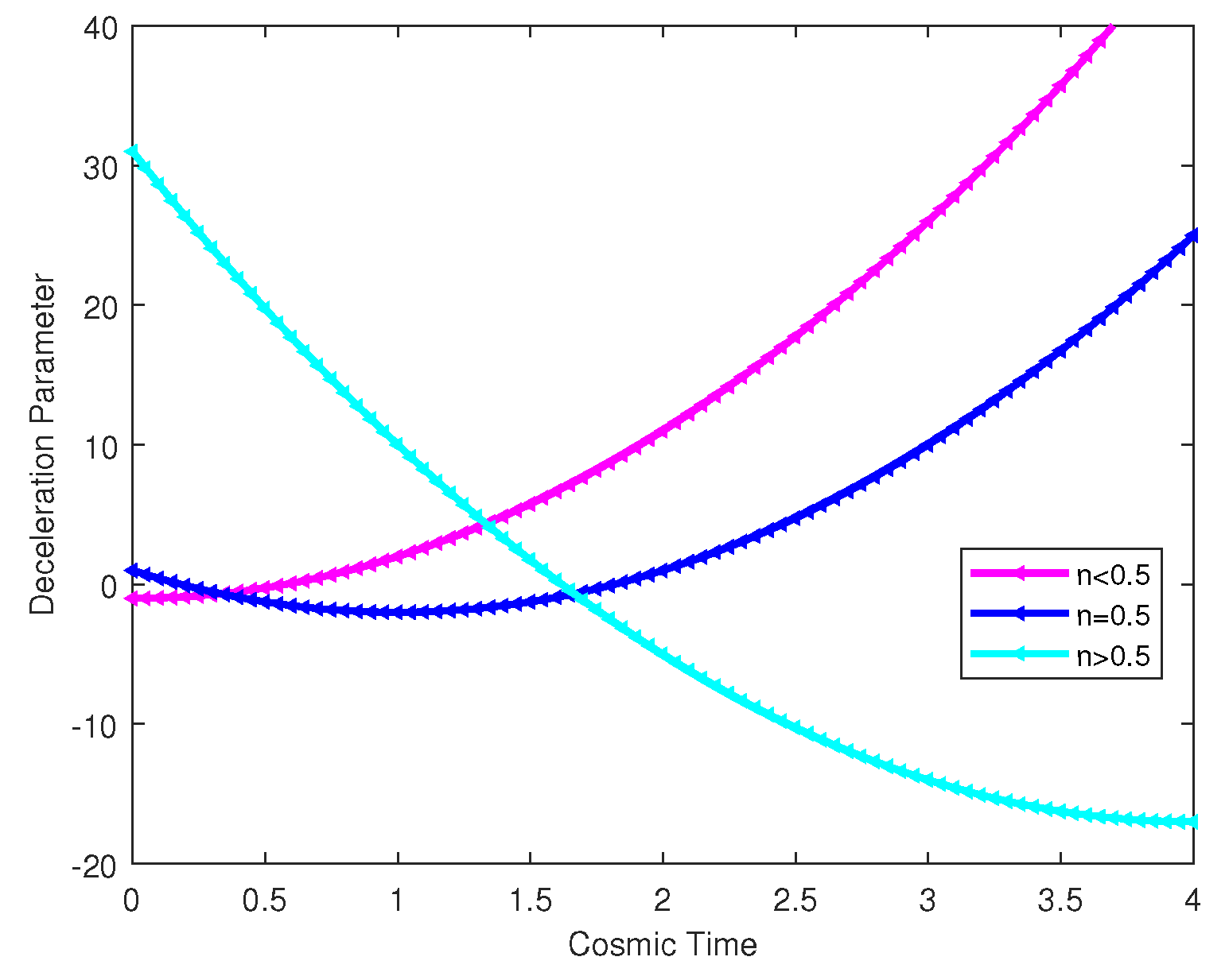
Figure 2.
Deceleration Parameter q with Redshift z
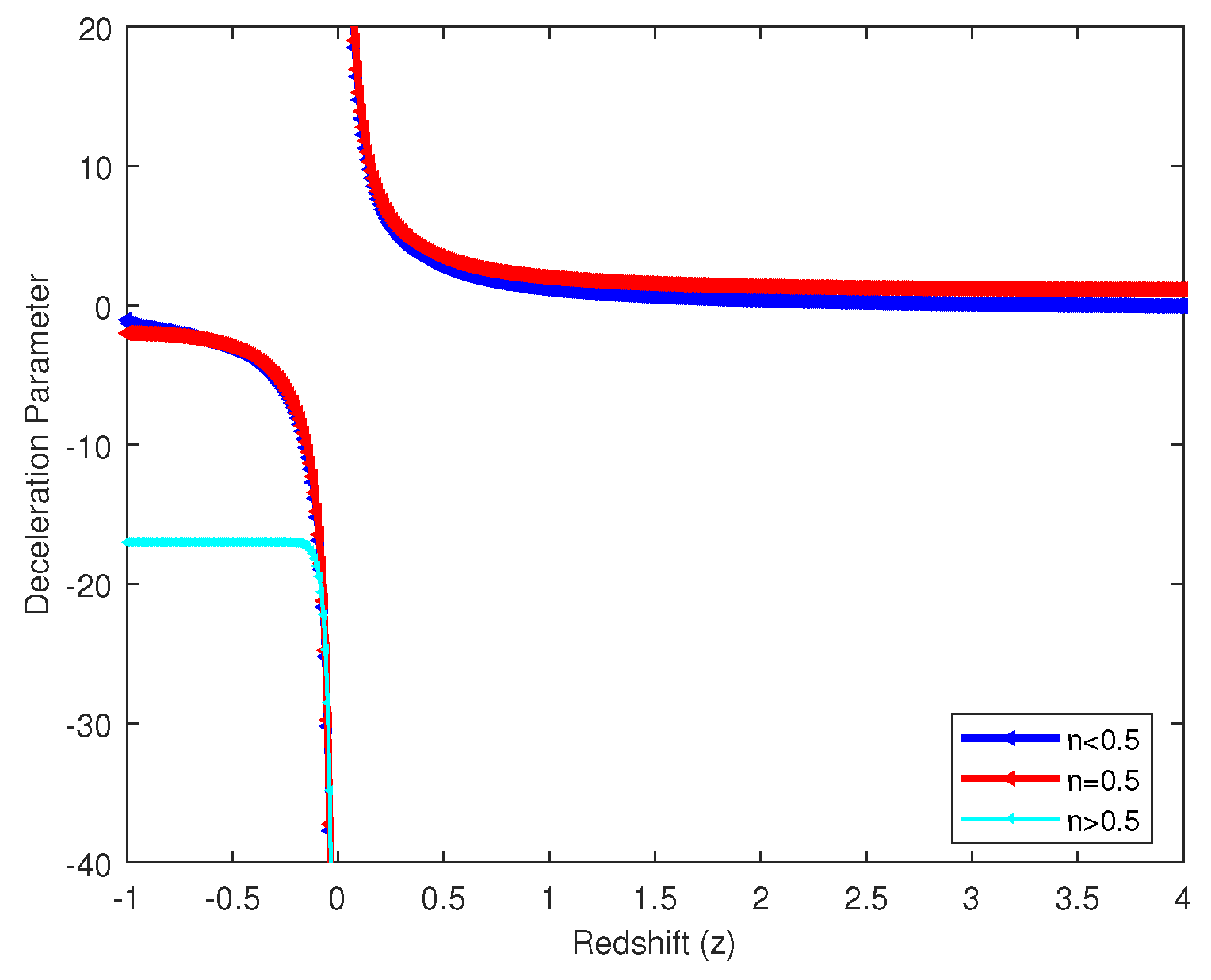
Figure 3.
Hubble Parameter H with cosmic time t
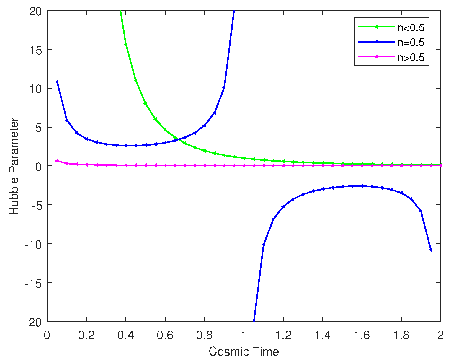
Figure 4.
Scale Factor s(t) variation with time
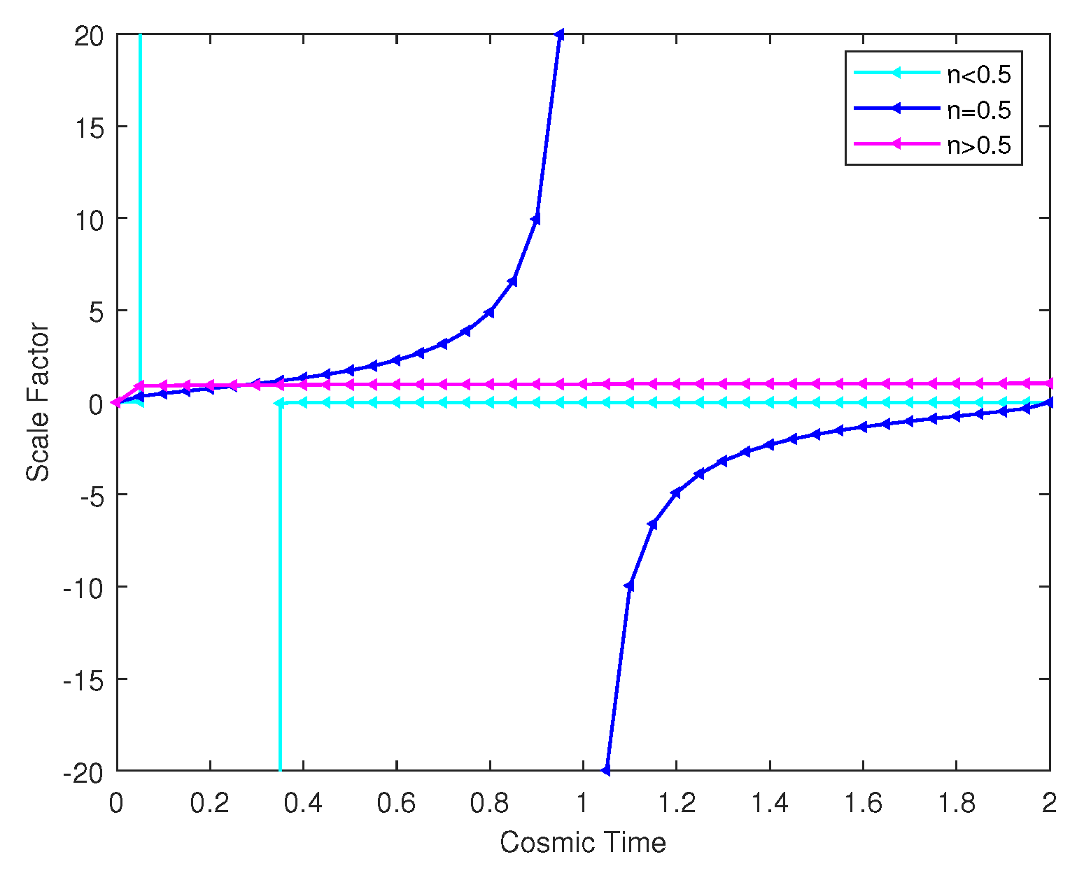
Figure 5.
Cosmological Constant at
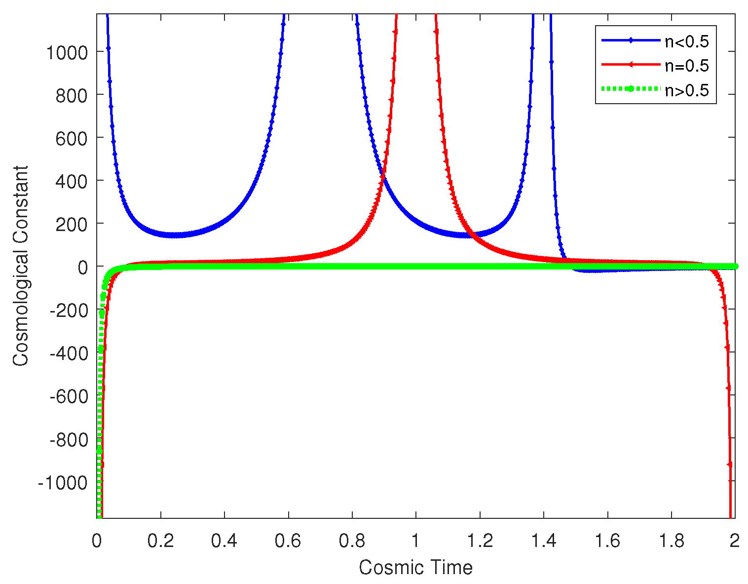
Figure 6.
Energy Density Variation at at
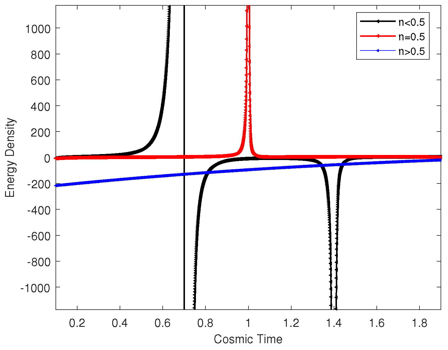
Figure 7.
Pressure P variation at
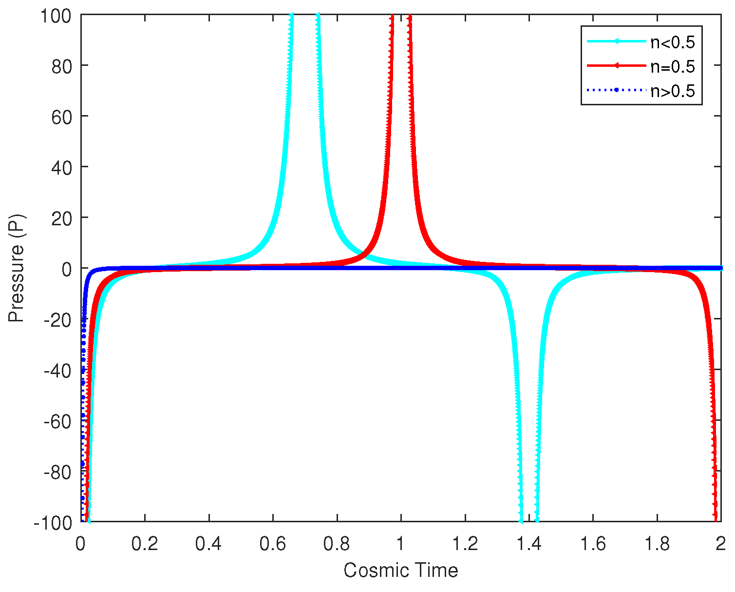
Figure 8.
EOS Parameter variation at
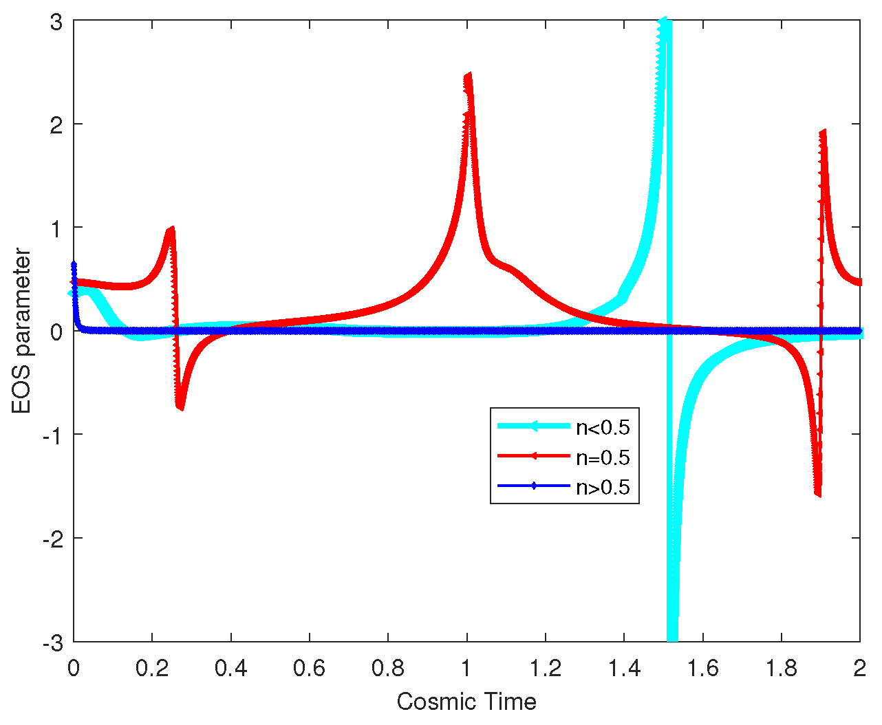
Figure 9.
Showing diagnostic variation at with redshift z
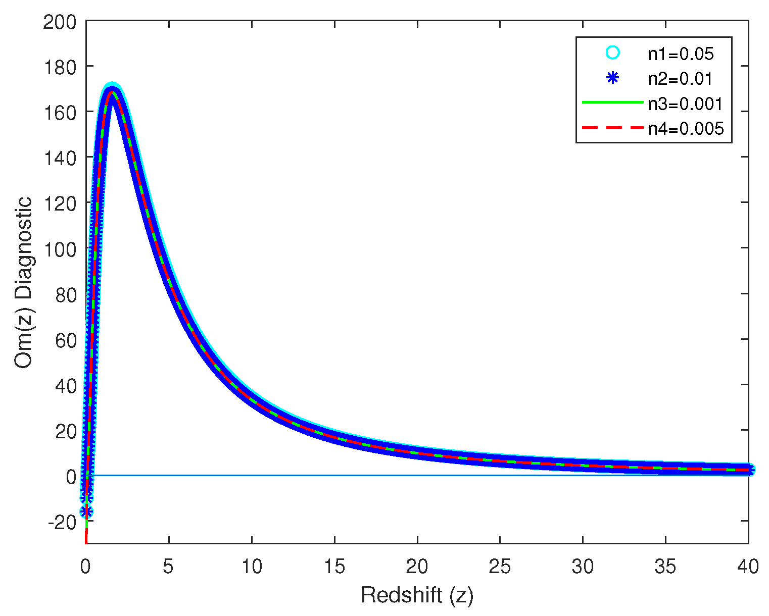
Figure 10.
Showing Energy density variation at .
Disclaimer/Publisher’s Note: The statements, opinions and data contained in all publications are solely those of the individual author(s) and contributor(s) and not of MDPI and/or the editor(s). MDPI and/or the editor(s) disclaim responsibility for any injury to people or property resulting from any ideas, methods, instructions or products referred to in the content. |
© 2023 by the authors. Licensee MDPI, Basel, Switzerland. This article is an open access article distributed under the terms and conditions of the Creative Commons Attribution (CC BY) license (http://creativecommons.org/licenses/by/4.0/).
Copyright: This open access article is published under a Creative Commons CC BY 4.0 license, which permit the free download, distribution, and reuse, provided that the author and preprint are cited in any reuse.


