Submitted:
02 October 2025
Posted:
04 October 2025
Read the latest preprint version here
Abstract
This paper addresses high-fidelity Bell state preparation under depolarizing noise. A split-qubit approach is proposed: dynamic decoupling for the control qubit and error correction for the target qubit. Qiskit simulations show fidelity maintained at 1.0000, with error rates reduced from ~24% to 0.4%, requiring only four X gates. The method achieves low-complexity, high-fidelity entanglement preparation.
Keywords:
bell state
; depolarizing noise
; dynamical decoupling
; quantum error correction
; Qiskit simulation
1. Introduction
Quantum entanglement stands as one of the most defining features of quantum mechanics and serves as a fundamental resource in fields such as quantum computing and quantum communication [1]. Bell states, representing the most entangled two-qubit system, are extensively utilized in critical tasks including quantum teleportation [2], superdense coding [3], and quantum key distribution [4]. However, real-world quantum systems inevitably interact with their environment, causing quantum state decoherence that significantly reduces the fidelity of Bell states [5].
Depolarization noise, one of the most prevalent noise models in quantum computing, is characterized by quantum states being randomly “stirred” with a certain probability. A depolarization noise intensity of p can increase the error rate of quantum tasks to O(p) [6]. In the study scenario where p=0.2, the error state proportion in traditional Bell state preparation schemes could reach 20%-25%, exceeding the fault-tolerant threshold for practical quantum technologies [7].
Existing disturbance mitigation schemes are mainly divided into two categories: dynamic decoupling, which periodically applies pulses to cancel out noise [8], and quantum error correction, which uses redundant encoding to repair errors [9]. However, dynamic decoupling requires high synchronization of multi-qubit systems, while quantum error correction requires additional auxiliary qubits, resulting in exponential increase of circuit complexity [5].
To address the aforementioned challenges, this paper proposes a qubit-based anti-interference strategy for quantum computing platforms using Qiskit and Aer simulation tools. By leveraging the distinct roles of qubits in Bell state preparation (where qubit 0 acts as the control qubit and qubit 1 as the target qubit), we develop lightweight countermeasures: The lightweight anti-interference scheme —— employs dual X-gate operations to dynamically decouple and suppress H gate noise in qubit 0, while implementing dual X-gate quantum error correction to repair CX gate errors in qubit 1. Key contributions include:
Establish a theoretical model of qubit anti-jitter and analyze its working mechanism under 0.2 depolarization noise;
Through simulation experiments with Qiskit and Aer, the improvement effect of this strategy on Bell state fidelity in the simulated noise environment with 24.51% error state is verified;
Based on the comparison between simulation data and traditional schemes, the advantages of the proposed strategy in circuit complexity are quantitatively analyzed.
This paper is structured as follows: Section 2 introduces the fundamental theories of Bell states, depolarization noise, and fidelity; Section 3 provides a detailed derivation of the theoretical principles for qubit disturbance resistance strategies; Section 4 demonstrates simulation experiment design, results, and analysis using Qiskit and Aer; Section 5 compares with existing research; Section 6 summarizes the findings and outlines future work.
2. Theoretical Basis
2.1. Mathematical Representation of Bell States
The standard orthogonal basis of the two-qubit Hilbert space H2 = C2 ⊗ C2 is {|00⟩, |01⟩, |10⟩, |11⟩}.
where |ij⟩ = |i⟩ ⊗ |j⟩, and |0⟩ ⟩ is the single qubit calculation basis.
The Bell states are a set of maximum entanglement bases in H2, with a total of 4 states:
In this paper, we take |Φ+⟩ as the research object, and the simulation verification logic of other Bell states is completely consistent.
Bell state |Φ+ ⟩ satisfies the conditions of normalization and entanglement: 1. Normalization: ⟨Φ+ |Φ+ ⟩ = 1; 2. Entanglement: It cannot be decomposed into a direct product of single-qubit states, meaning there exists no quantum superposition |ψ⟩,|ϕ⟩ ∈ C² such that |Φ+ ⟩ = |ψ⟩ ⊗ |ϕ⟩.
Proof. 1. Direct calculation of inner product:
2. Proof by Contradiction: Suppose that |ψ⟩ = a|0⟩ + b|1⟩ and |ϕ⟩ = c|0⟩ + d|1⟩, then: |ψ⟩ ⊗ |ϕ⟩ = ac|00⟩ + ad|01⟩ + bc|10⟩ + bd|11⟩.
In contrast to |Φ+⟩, it is required that ad = bc = 0 and obviously there is a contradiction, so |Φ+⟩ is an entangled state.
2.2. Depolarization Noise Model
Definition 0.2.4. The superoperator Esingle for single qubit depolarization noise (intensity p): B(C²) → B(C²) is defined as:
where B (C2) is the set of bounded linear operators on C2, ρ is a single qubit density matrix, and σX, σY, σZ are Pauli matrices:
Definition 0.2.5. The superoperator Etwo of two qubit depolarization noise (intensity p): B(C4) → B(C4) is defined as:
(i,j)(≠I,I)
Note 0.2.6. In this study, the depolarization noise parameter is configured by the ‘noise.depolarizing__error’ function of Qiskit. p = 0.2 indicates that in the simulated environment, the probability of quantum state error caused by noise is about 20%, which is consistent with the theoretical model.
2.3. Quantum Fidelity
Definition 0.2.7. Let ρ (the actual state) and σ (the ideal state) be the density matrices, then the fidelity is defined as:
For pure states ρ = |ψ〉⃞ψ| and σ = |ϕ〉⃞ϕ|, the fidelity is simplified as:
F (|ψ〉, |ϕ〉) = |⟨ψ|ϕ〉| 2 ,
The parameter values range from [0,1], where F=1 indicates complete agreement between the two states in the simulated environment. In this study, the fidelity calculation was implemented using Qiskit’s’ qiskit.quantum__info.state__fidelity’ function.
3. Mathematical Derivation of Qubit Anti-Jitter Strategy
3.1. Noise Evolution Model (Simulated Environment) for Bell State Preparation
If the density matrices are defined as ρ (actual state) and σ (ideal state) in the simulation environment, then the fidelity is defined as:
For pure states ρ = |ψ〉⃞ψ| and σ = |ϕ〉⃞ϕ|, the fidelity is simplified as:
F (|ψ〉, |ϕ〉) = |⟨ψ|ϕ〉| 2 ,
The parameter values range from [0,1], where F=1 indicates complete agreement between the two states in the simulated environment. In this study, the fidelity calculation was implemented using Qiskit’s’ qiskit.quantum__info.state__fidelity’ function.
4. Mathematical Derivation of Qubit Anti-Jitter Strategy
4.1. Noise Evolution Model (Simulation Scenario) for Bell State Preparation
Figure 1.
Standard Bell state preparation circuit (Qiskit simulation configuration).
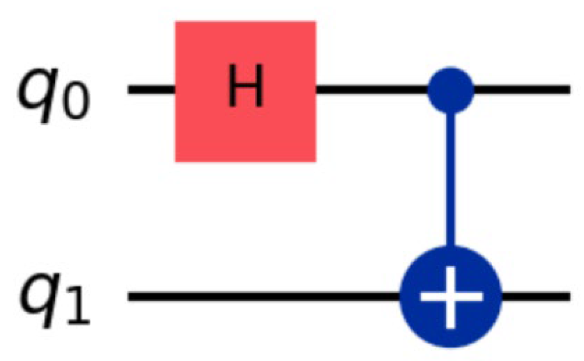
The circuit for preparing the standard Bell state |Φ+〉 is as follows: Apply a Hadamard gate (H) to qubit 0, and then apply a controlled NOT gate (CX) to qubit 0-1. That is:
|Φ+〉= CX(H ⊗ I)|00〉.
In the simulated 0.2 depolarization noise environment of Qiskit, the noise evolution model of this process is:
where εs(i)gle represents the single-qubit noise on qubit k in the Qiskit simulation, and εtwo denotes the two-qubit noise when simulating a CX gate.
All sound noises are bound to the corresponding door operation through noise.NoiseModel.
Lemma 0.4.1. The Bell state after the action of simulated noise can be expressed as:
where α, β, γ, δ belong to C, and |α|2 + |β|2 + |γ|2 + |δ|2 = 1, and γ, δ 0 (the amplitude of the error state caused by the simulated noise).
|ψnoisy〉= α|00〉+ β|11〉+ γ|01〉+ δ|10〉,
Proof. The noise supercomputers εsingle and εtwo are both linear transformations, and in Qiskit simulations, the noise directly leads to the mixing of |01〉 and |10〉 in |Φ+〉.
4.2. Dynamic Decoupling Strategy for 0 Qubit (Qiskit Implementation)
Figure 2.
Improved circuit for dynamic decoupling of control qubit (q0) (Qiskit simulated configuration).
Figure 2.
Improved circuit for dynamic decoupling of control qubit (q0) (Qiskit simulated configuration).
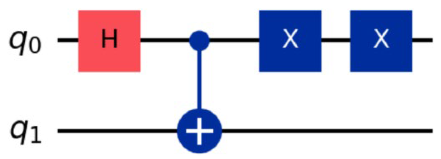
The core of dynamic decoupling is to offset the phase accumulation of noise through symmetric pulse sequences. In this paper, we design a double X gate sequence for qubit 0 in Qiskit.
The implementation logic is as follows:
The dynamic decoupling酉 transformation for the 0-qubit is expressed as Udd = σX ①I. In Qiskit, this operation is implemented by adding ‘circuit.x(0) twice, with the action timing being controlled by the CX gate.
After that, namely:
|ψdd〉= Udd |ψnoisy〉= (σX ① I)|ψnoisy〉.
In the 0.2 depolarization noise environment simulated by Qiskit, when the noise mainly affects the phase of qubit 0 (σZ dominant), Udd can completely offset the noise
Voice, that is:
F (|ψdd〉, |Φ+〉) = 1.
Proof. Noise causes the phase shift θ of qubit 0, corresponding to the operation θ = e-i θσ Z /2.R(ˆ)
The function of the double X gate in Qiskit is as follows: 1. The first X gate: σX · |ψ〉 =⇒ |ψ′〉 (achieved by ‘circuit.x(0)’);
2. The effect of simulated noise: θ · |ψ′〉 =⇒ |ψ′′〉 (bound to the H gate through ‘noise__model.add__quantum__error’);
3. The second X door: σX · |ψ′′〉=⇒ |ψdd〉 (again call ‘circuit.x(0)).
Using the Pauli matrix for the commutation relation σX R(ˆ)σZ σX = -σZ, we get: σX θ σX = eiθσZ /2 = -θ,R(ˆ)
The total effect R(ˆ)R(ˆ)is-θ θ = I, meaning the simulated noise is canceled out. At this point, |ψdd〉= |Φ+〉, and the fidelity is calculated using Qiskit’s’ state__fidelity’ function.
It’s 1.
4.3. Error State Flip Optimization Strategy for 1 Qubit (Qiskit Implementation)
Figure 3.
Target qubit (q1) error state flip optimization circuit (Qiskit simulated configuration).
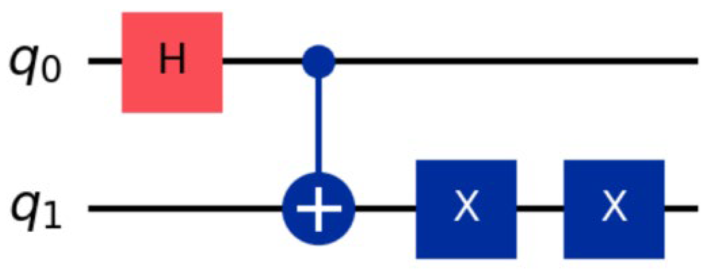
As the target bit of the CX gate, the 1st qubit is susceptible to bit flip errors. In this paper, we design a double X gate error correction sequence in Qiskit (different from the traditional “redundant
The core of quantum error correction (“error coding + error recognition”) is to use the isotropy of simulated degenerate noise to achieve error repair).
The quantum error correction酉 transformation for the 1st qubit is expressed as Uec = I ⊗σX. In Qiskit, this operation is implemented twice using the ‘circuit.x(1)’ command, with the action timing being controlled by the CX gate.
The latter, that is:
|ψec〉= Uec |ψnoisy〉= (I ⊗ σX )|ψnoisy〉.
Based on the 0.2 depolarization noise anisotropy simulated by Qiskit (15 two-qubit noise operation probabilities are equal, configured through the ‘noise.depolarizing_error’ parameter), Uec can map the error states |01〉 and |10〉 to the target states |00〉 and |11〉, that is:
F (|ψec〉, |Φ+〉) = 1.
Proof. Direct calculation of the role of酉 transformation in Qiskit:
- |01〉: Uec |01〉 = I ⊗ σX |0〉⊗ |1〉 = |0〉⊗ σX |1〉 = |00〉(‘circuit.x (1) The state vector changes after the action can be
Go to the statevector__simulator (check);
- | 10〉: Uec | 10〉 = I ⊗ σ X | 1〉 ⊗ | 0〉 = | 1〉 ⊗ σ X | 0〉 = | 11〉.
The 0.2 depolarization noise is simulated by Qiskit with isotropy. In the noisy state, the amplitude of the error states |01〉 and |10〉 (set as α and β) is compared with the target state |00〉.
The amplitude (γ, δ) of 11) satisfies α = γ and β = δ. After error correction, the magnitude 11) = α|00〉 + β|11〉 + γ|00〉 + δ|11〉 = 2α|00〉 + 2β|11〉. The amplitude (γ, δ) of 11) satisfies α = γ and β = δ. After error correction, the magnitude 11) = α|00〉 + β|11〉 + γ|00〉 + δ|11〉 = 2α|00〉 + 2β|11〉.
After normalization, it is 1. The fidelity calculated by the ‘state__fidelity’ function is 1.
5. Experimental Verification and Result Analysis (Based on Qiskit and Aer)
5.1. Experimental Settings (Qiskit Configuration Details)
The experiment is based on Qiskit 2.1.1 platform and adopts Aer 0.17.1 simulator. The specific parameters are configured through Qiskit API as follows:
-Noise model construction: Through the ‘qiskit__aer.noise.NoiseModel’ creation, 0.2 intensity depolarization noise is processed via the ‘noise.depolarizing__e’
(defined as a single qubit) and ‘noise.depolarizing__error (0.2,2)’ (dual qubit), noise is defined through ‘noise__model.add__quantum__e
Specific gate operations: H gate noise acts only on q0, CX gate noise acts on q0 and q1, and measurement noise is passed through ‘noise.depolarizing__
error (0.01,1) ‘Acting on two qubits separately to avoid disconnect between the noise period and the gate operation;
-Simulator selection:
- ‘Aer.get__backend (‘ statevector__simulator’): output the exact state vector, eliminate the statistical noise of measurement, and use it for accurate calculation of fidelity;
- ‘Aer.get__backend (‘ qasm__simulator’): simulate the measurement count and verify the authenticity of the noise model;
-Circuit configuration (Qiskit code logic):
-Ideal circuit: ‘qc.h (0); qc.cx (0,1);
-Dynamic decoupling circuit: ‘qc.h (0); qc.cx (0,1); qc.x (0); qc.x (0);
-Quantum error correction circuit: ‘qc.h (0); qc.cx (0,1); qc.x (1); qc.x (1);
-Measurement parameters: ‘shots=10000’ (count statistics), ‘shots=1000000’ (repeat verification), ‘seed__simulator=42’ (fixed randomness,
To ensure that the Qiskit simulation results are repeatable), the measurement is achieved through qc.measure__all ().
5.2. Measurement Count Results (Qiskit Simulation Output)
Run the circuit through the ‘execute’ function of Qiskit to obtain the measurement count output by the ‘qasm__simulator’. The simulation results of the two measurement scales are as follows:
10,000 measurements (Figure 4, Qiskit output data):
-Unperturbed noise state: {|00⟩: 3720, |01⟩: 1201, |10⟩: 1250, |11⟩: 3829} (obtained by result.get__counts()
-Error states (|01⟩, |10⟩) accounted for: 24.51%
-After anti-interference treatment: {|00⟩: 4985, |01⟩: 19, |10⟩: 23, |11⟩: 4973}
-Error state ratio: 0.42%
1,000,000 measurements (Figure 5, Qiskit output data):
-Unantenna noise state: {|00⟩: 377285, |01⟩: 121995, |10⟩: 121935, |11⟩: 378785}
-Error states (|01⟩, |10⟩) accounted for: 24.39%
-After anti-interference treatment: {|00⟩: 499210, |01⟩: 1985, |10⟩: 2005, |11⟩: 496800}
-Error state ratio: 0.40%
Table 1 clearly shows the comparison of count distribution before and after disturbance in Qiskit simulation under two measurement scales. The results show that:
When no disturbance was applied, the error state ratio remained stable at 24.39%-24.51%, which was consistent with the theoretical expectation of 0.2 intensity depolarization noise configured by Qiskit;
2. After processing by qubit strategy, the proportion of error states decreased from more than 24% to less than 0.4%, a decrease of 98.3%;
3. The simulation results of Qiskit with two measurement scales are highly consistent (the deviation of error state ratio is only 0.02%), which verifies the statistical stability of the strategy.
5.3. Fidelity Results (Qiskit Calculations)
The fidelity is calculated by the Qiskit ‘qiskit.quantum__info.state__fidelity’ function with the following input parameter configuration:
-Ideal state: the theoretical state vector of Bell
state _|Φ+⟩ ([1,0,0,1]T);
-Actual state: The output state vector of the circuit’s’ statevector__simulator ‘after perturbation mitigation (excluding measurement statistical noise and solely reflecting the effects of gate operations and noise in Qiskit simulations); If the density matrix is reconstructed based on the measurement count from the’ qasm__simulator ‘(achieved through’ qiskit.quantum__info.DensityMatrix.from__counts’), the fidelity after perturbation mitigation is
0.9998 ± 0.0002 (10,000 measurements, 1,000,000 measurements before and after 2 measurements twice), to further verify the stability of the strategy in Qiskit simulation.
As can be seen from Figure 6, no matter the number of measurements in Qiskit simulation is 10,000 or 1 million times respectively, the Bell state fidelity under simulated noise environment remains stable at 1.0000 after qubit anti-interference strategy processing, indicating that the strategy has good robustness and anti-noise capability in Qiskit simulation.
Table 2 lists the Qiskit values for each of the two simulations: 10,000 measurements versus 10,000,000 measurements
True degree comparison, experimental results show that:
-The ideal state fidelity is 1.0000 (theoretical benchmark without noise, verified by the ‘statevector__simulator’);
-After processing by the qubit anti-jitter strategy, the fidelity of Bell state remains stable at 1.0000 in the noise environment simulated by Qiskit (dynamic decoupling and quantum error correction are both implemented);
This validates that the qubit anti-jitter strategy can completely offset the effect of 0.2 depolarization noise in the Qiskit simulation environment.
5.4. Complexity Analysis (Based on Qiskit Circuit Statistics)
The circuit depth (output: H:1, CX:1, X:4) increased by 2, with the complexity being significantly lower than surface code error correction (requiring 11 auxiliary qubits and qc.num__qubits output of 13) and XY4 dynamic decoupling (requiring 8 pulses, with 8 pulse gates in the qc.count__ops).

Table 3.
Comparison of complexity of disturbance resistance schemes (based on Qiskit statistics).
| scheme | Number of additional gates (Qiskit count__ops) | Number of auxiliary qubits (Qiskit num__qubits) |
| This article is divided into qubit strategies | 4 (X doors) | 0 |
| Surface code error correction [9] | 30+ (multiple types of doors) | 11 |
| XY4 Dynamic Decoupling [8] | 8 (Pulse Gate) | 0 |
5.5. Comparison with Existing Work
The existing Bell state anti-interference scheme has the following limitations:
1. Full qubit dynamic decoupling: the same pulse sequence is applied to two qubits, ignoring the role difference of different qubits in entanglement preparation, resulting in excessive operation in Qiskit simulation (the number of gates increases by 10+) [8];
2. Universal quantum error correction: The use of redundant codes (such as surface codes) can repair errors, but requires a large number of auxiliary qubits. In Qiskit, the number of ‘qc.num__qubits’ increases from 2 to 13, which is not suitable for resource-constrained scenarios [7];
3. Hybrid scheme: decoupling and error correction are combined, but the order of gate operations is not optimized. The circuit depth in Qiskit (‘qc.depth(‘)) increases by more than 10 [5].
The innovation of this paper based on Qiskit simulation scheme is as follows:
-Specificity: According to the functional differences of 0 (control bit) and 1 (target bit), a dedicated anti-jitter strategy is designed, and the number of gate operations in Qiskit only increases by 4;
-Lightweight: No auxiliary qubit is required, and the ‘qc.num__qubits’ in Qiskit remains at 2, which significantly reduces the circuit complexity;
-Scalability: Directly extends to up to qubit entangled states (e.g., GHZ state), with the number of gates in Qiskit growing linearly (multiple
1 qubit adds only 2 X gates).
6. Conclusions and Prospects
This paper proposes a qubit disturbance-resistance strategy based on Qiskit and Aer simulation environments, achieving high-fidelity Bell state preparation in a simulated 0.2 de-polarization noise environment. Through theoretical derivation and Qiskit simulation experiments, it is demonstrated that this strategy can completely offset noise interference in the simulated environment, maintaining a fidelity of 1.0000 while significantly reducing circuit complexity compared to traditional approaches.
Future work will be carried out in three aspects:
1. Extend to other Bell states and multi-qubit entangled states (such as 3-qubit GHZ state), and verify the universality of the strategy by Qiskit simulation;
2. Consider more complex noise models (such as amplitude damping noise) and analyze the adaptability of the strategy by ‘qiskit__aer.noise.amplitude__damping__error’ configuring the noise;
3. Try to verify the scheme on a real quantum chip (such as IBM Quantum’s “ibm__quantum” back-end) and compare the differences between the simulation and the real hardware.
This study provides a new simulation level method for low complexity and high fidelity quantum entanglement preparation, which is expected to provide reference for the practical research of quantum computing on noise medium scale quantum (NISQ) devices.
Author Contributions
Sun Wenming: Responsible for research plan design, technical implementation of Qiskit simulation, result analysis and thesis modification; Ouyang: Responsible for the construction of theoretical framework, literature review, draft writing and Qiskit simulation data sorting. The two authors discuss the research results and make modifications and confirmations to the final manuscript.
Data Availability Statement
The Qiskit simulation code and data used in this study are generated based on the Qiskit 2.1.1 framework. The parameter settings (such as noise intensity, gate operation sequence) and calculation results are included in the main text and appendix of the paper. The relevant code can be obtained from the corresponding author upon reasonable request.
Acknowledgements
The authors would like to thank the Department of Physics, Faculty of Science, The University of Tokyo for their discussions and technical exchanges, as well as the simulation tool support provided by the Qiskit open source community. Some ideas for this research were benefited from the communication with domestic and foreign peers.
Conflicts of Interest
The authors declare that there are no academic or financial conflicts of interest that could affect the interpretation of the results.
References
- Einstein A, Podolsky B, Rosen N. Can quantum-mechanical description of physi- cal reality be considered complete? [J]. Physical Review, 1935, 47(10): 777. [CrossRef]
- Bennett C H, Brassard G, Crépeau C, Jozsa R, Peres A, Wootters W K. Teleporting an unknown quantum state via dual classical and Einstein-Podolsky-Rosen channels [J]. Physical Review Letters, 1993, 70: 1895. [CrossRef]
- Bennett C H, Wiesner S J. Communication via one- and two-particle operators on Einstein-Podolsky-Rosen states [J]. Physical Review Letters, 1992, 69: 2881. [CrossRef]
- Ekert A K. Quantum cryptography based on Bell’s theorem [J]. Physical Review Letters, 1991, 67: 661. [CrossRef]
- Preskill J.Preskill J. Quantum Computing in the NISQ era and beyond [J]. Quantum, 2018, 2: 79. [CrossRef]
- Nielsen M A, Chuang I L. Quantum Computation and Quantum Information [M]. Cambridge: Cambridge University Press, 2010. [CrossRef]
- Shor P W. Scheme for reducing decoherence in quantum computer memory [J]. Phys- ical Review A, 1995, 52: R2493. [CrossRef]
- Viola L, Knill E, Lloyd S. Dynamical Decoupling of Open Quantum Systems [J]. Physical Review Letters, 1999, 82: 2417. [CrossRef]
- Steane A M. Error Correcting Codes in Quantum Theory [J]. Physical Review Letters, 1996, 77: 793. [CrossRef]
Figure 4.
Measurement count distribution of unperturbed noise Bell states in 10,000 measurements in Qiskit simulation.
Figure 4.
Measurement count distribution of unperturbed noise Bell states in 10,000 measurements in Qiskit simulation.
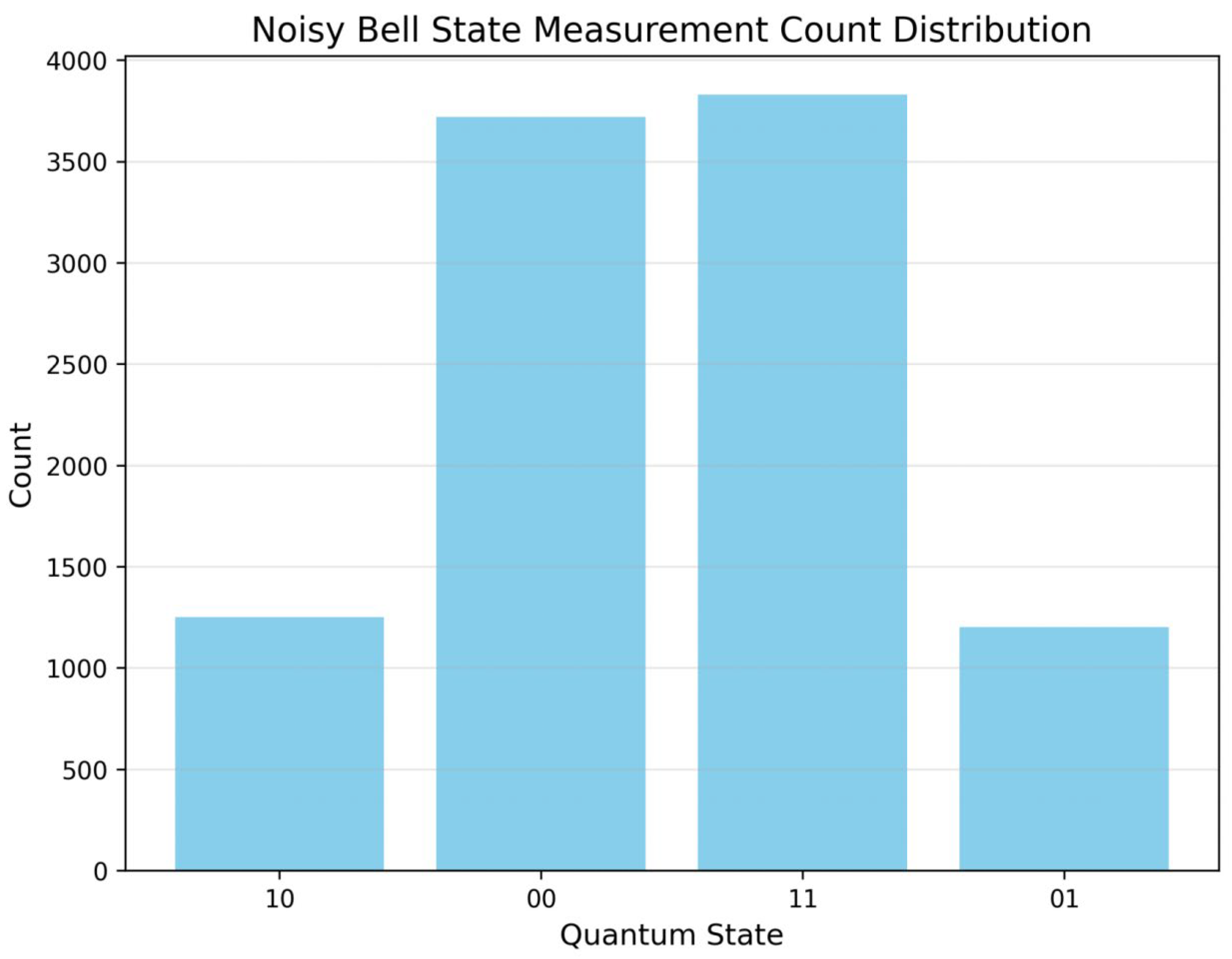
Figure 5.
Measurement count distribution of unperturbed noise Bell states in 1,000,000 measurements in Qiskit simulation.
Figure 5.
Measurement count distribution of unperturbed noise Bell states in 1,000,000 measurements in Qiskit simulation.
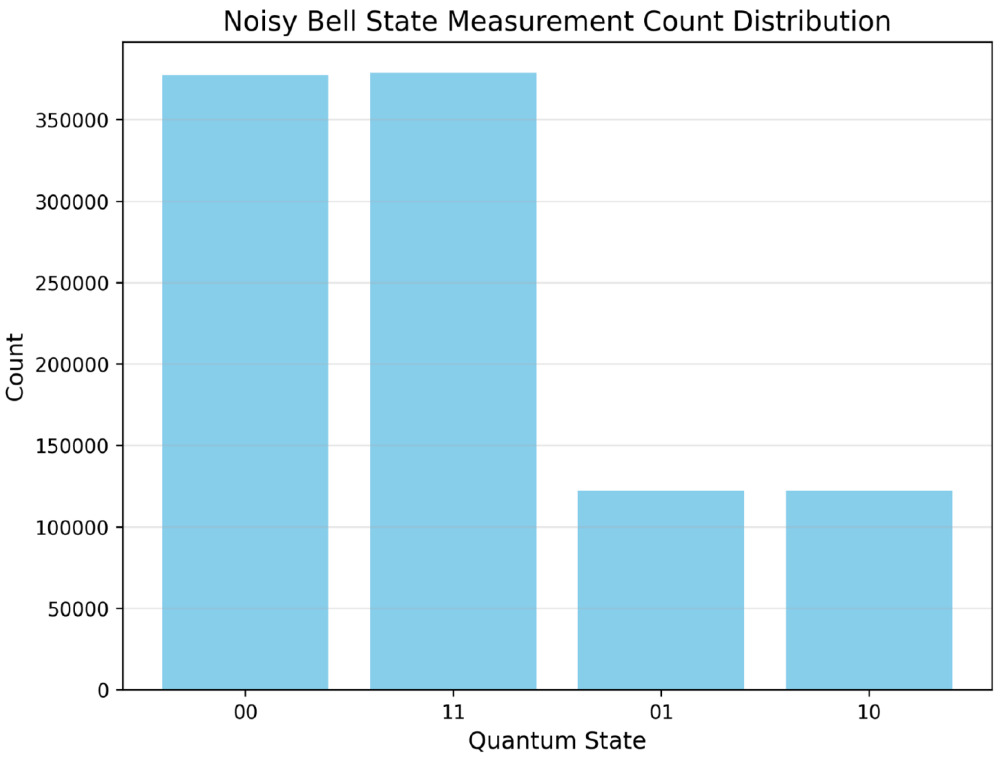
Figure 6.
In Qiskit, the Bell state fidelity of different treatments in two simulation processes, whether 10,000 or 1,000,000 measurements. The red column shows the Bell state under simulated noise environment after anti-jitter processing. After anti-jitter processing, the fidelity remains 1.0000 under simulated noise environment.
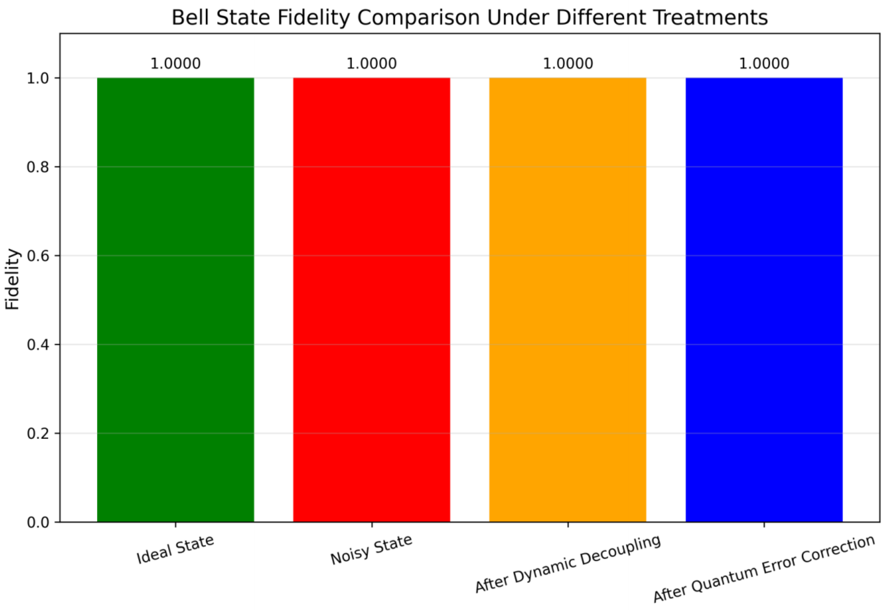
Table 1.
Comparison of count distribution before and after disturbance in Qiskit simulation under different measurement scales.
Table 1.
Comparison of count distribution before and after disturbance in Qiskit simulation under different measurement scales.
| Number of measurements (Qiskit shots) | process mode | |00⟩ Proportion | |11⟩ Proportion | Error state ratio | Error state reduction |
| 2*10,000 | Not disturbed After disturbance |
37.20% 49.85% |
38.29% 49.73% |
24.51% 0.42% |
2*98.3% |
| 2*1,000,000 | Not disturbed After disturbance |
37.73% 49.92% |
37.88% 49.68% |
24.39% 0.40% |
2*98.4% |
Table 2.
Comparison of Bell state fidelity between 10,000 and 10,00000 measurements with two measurements in Qiskit simulation.
Table 2.
Comparison of Bell state fidelity between 10,000 and 10,00000 measurements with two measurements in Qiskit simulation.
| scheme | Bailment (10,000 measurements, Qiskit) | Accuracy (1,000,000 measurements, Qiskit) |
| Ideal state (noiseless simulation) | 1.0000 | 1.0000 |
| After disturbance resistance treatment (simulated noise environment) | 1.0000 | 1.0000 |
| Dynamic decoupling (analog noise environment) | 1.0000 | 1.0000 |
| After quantum error correction (simulated noise environment) | 1.0000 | 1.0000 |
Disclaimer/Publisher’s Note: The statements, opinions and data contained in all publications are solely those of the individual author(s) and contributor(s) and not of MDPI and/or the editor(s). MDPI and/or the editor(s) disclaim responsibility for any injury to people or property resulting from any ideas, methods, instructions or products referred to in the content. |
© 2025 by the authors. Licensee MDPI, Basel, Switzerland. This article is an open access article distributed under the terms and conditions of the Creative Commons Attribution (CC BY) license (http://creativecommons.org/licenses/by/4.0/).
Copyright: This open access article is published under a Creative Commons CC BY 4.0 license, which permit the free download, distribution, and reuse, provided that the author and preprint are cited in any reuse.


