Connecting the FLRW and Schwarzschild Singularities

1. Introduction

The Big Bang and Schwarzschild singularities are two of the most mysterious objects in General Relativity. One of the big questions associated with these singularities is: What happened before the Big Bang and what happened after the Schwarzschild singularity?

When the Schwarzschild metric is expressed in Kruskal-Szekeres coordinates, we see that there are actually two singularities in the metric. By similarly expressing the FLRW metric in Kruskal-Szekeres coordinates, it will be shown that the FLRW metric also has two singularities, which are colocated with the Schwarzschild singularities. But under closer inspection, we find that even though the singularities are colocated on that coordinate chart, they are not colocated in spacetime. Instead, we find that the interior Schwarzschild manifold curves away from the FLRW/Exterior Schwarzschild manifold and they intersect at the event horizon.

Once this geometry is made clear, it becomes clear that there is more to these manifolds than is currently known. In particular, it becomes clear that there is a collapsing Universe in which White Holes are the source of high entropy matter and the FLRW singularity is the sink into which this Universe collapses.

In the end, we are able to chart a path between all the singularities and what emerges is an eternal cycle that is powered by Black and White Holes.

2. Transforming the Coordinates of the FLRW Spacetime

The flat FLRW metric is typically given in the following form:

$$d{\tau }^2=d{t}^2-a{\left(t\right)}^{2}d{r}^2-a{\left(t\right)}^{2}d{\Omega }^2$$

(1)

In this paper, we will focus on the $dt$ and $dr$ terms in the metric and mostly ignore the azimuthal term. We wish to express the metric in Kruskal-Szekeres coordinates in order to compare the Schwarzschild and FLRW singularities. The first step is to express the FLRW metric in a form that resembles the Schwarzschild metric. We do this by changing the time coordinate:

$$\begin{array}{c}\hfill dt={\displaystyle \frac{1}{a\left(t\right)}}d{t}^{\prime }\end{array}$$

(2)

And from this we see that:

$$\begin{array}{c}\hfill t^{\prime }=\int a\left(t\right)dt\end{array}$$

(3)

Since we have $t^{\prime }$ as a function of t, we can express the scale factor a as a function of $t^{\prime }$ instead of t and rewrite the flat FRW metric as (without the angular term):

$$d{\tau }^2={\displaystyle \frac{1}{a{\left(t^{\prime }\right)}^2}}d{t}^{\prime 2}-a{\left(t^{\prime }\right)}^{2}d{r}^2$$

(4)

Contrast this with the interior Schwarzschild metric given below:

$$d{\tau }^2={\displaystyle \frac{1}{\frac{r_s}{r}-1}}d{r}^2-\left({\displaystyle \frac{r_s}{r}}-1\right)d{t}^2$$

(5)

Now, it is important to keep in mind that in the interior Schwarzschild metric, r is the timelike coordinate and t is the spacelike coordinate, which is opposite to the FLRW coordinate labels.

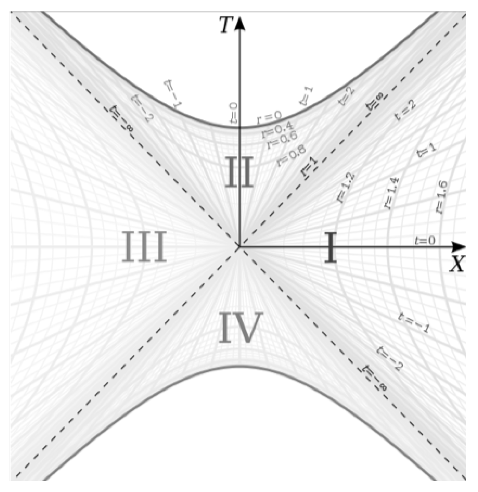
Comparing equations 4 and 5, we see that (when ignoring the angular terms), they have the same form with a time-dependent scale factor multiplying the spacelike coordinate and the inverse of the scale factor multiplying the timelike coordinate. This is interesting because the Schwarzschild metric, when expressed in Kruskal-Szekeres coordinates, is shown to have two ’branches’ in its geometry. In Schwarzschild coordinates, the Schwarzschild metric has an exterior solution and an interior solution. In Kruskal-Szekeres coordinates, we get an additional exterior region and an additional interior region, as can be seen in the Kruskal-Szekeres coordinate chart below [1]:

So the metric in Schwarzschild coordinates gives regions I and II in Figure 1 and when converting to Kruskal-Szekeres coordinates, we get the additional regions III and IV. Since the metrics have such similar structures, we’d like to see if we can get an additional branch for the flat FRW metric by doing a similar coordinate transformation for that metric.

We will define the new coordinates for the FRW metric as follows:

$$\begin{array}{c}\hfill T=f\left(t^{\prime }\right)cosh\left({\displaystyle \frac{r}{\mu }}\right)\\ \hfill X=f\left(t^{\prime }\right)sinh\left({\displaystyle \frac{r}{\mu }}\right)\end{array}$$

(6)

Where $\mu$ is a constant with units of time. Our goal is to find the function $f\left(t^{\prime }\right)$ for the FLRW metric. If we take the differentials of T and X we get:

$$\begin{array}{c}\hfill dT=\dot{f}\left(t^{\prime }\right)cosh\left({\displaystyle \frac{r}{\mu }}\right)d{t}^{\prime }+{\displaystyle \frac{f\left(t^{\prime }\right)}{\mu }}sinh\left({\displaystyle \frac{r}{\mu }}\right)dr\\ \hfill dX=\dot{f}\left(t^{\prime }\right)sinh\left({\displaystyle \frac{r}{\mu }}\right)d{t}^{\prime }+{\displaystyle \frac{f\left(t^{\prime }\right)}{\mu }}cosh\left({\displaystyle \frac{r}{\mu }}\right)dr\end{array}$$

(7)

Where $\dot{f}\left(t^{\prime }\right)$ is ${\displaystyle \frac{df}{d{t}^{\prime }}}$. Next, we find $d{T}^2-d{X}^2$:

$$\begin{array}{c}\hfill d{T}^2-d{X}^2=\dot{f}{\left(t^{\prime }\right)}^{2}d{t}^{\prime 2}-{\left({\displaystyle \frac{f\left(t^{\prime }\right)}{\mu }}\right)}^{2}d{r}^2\end{array}$$

(8)

Next, we assume the metric in these coordinates will have the form:

$$\begin{array}{c}\hfill d{\tau }^2=g{\left(t^{\prime }\right)}^2\left[d{T}^2-d{X}^2\right]\end{array}$$

(9)

Comparing equations 8 and 9 with equation 4, we can derive the constraints we need to determine $f\left(t^{\prime }\right)$ and $g\left(t^{\prime }\right)$. First, we recognize that:

$$\begin{array}{cc}\hfill g\left(t^{\prime }\right)\dot{f}\left(t^{\prime }\right)& ={\displaystyle \frac{1}{a\left(t^{\prime }\right)}}\hfill \\ \hfill \dot{f}\left(t^{\prime }\right)& ={\displaystyle \frac{1}{g\left(t^{\prime }\right)a\left(t^{\prime }\right)}}\hfill \end{array}$$

(10)

And,

$$\begin{array}{cc}\hfill g\left(t^{\prime }\right){\displaystyle \frac{f\left(t^{\prime }\right)}{\mu }}& =a\left(t^{\prime }\right)\hfill \\ \hfill g\left(t^{\prime }\right)& ={\displaystyle \frac{a\left(t^{\prime }\right)\mu }{f\left(t^{\prime }\right)}}\hfill \end{array}$$

(11)

If we substitute equation 11 into equation 10, we get the following differential equation for $f\left(t^{\prime }\right)$:

$$\begin{array}{c}\hfill \dot{f}\left(t^{\prime }\right)={\displaystyle \frac{1}{\mu }}{\displaystyle \frac{f\left(t^{\prime }\right)}{a{\left(t^{\prime }\right)}^2}}\end{array}$$

(12)

Equation 12 is a differential equation that allows us to solve for $f\left(t^{\prime }\right)$ given $a\left(t^{\prime }\right)$.

Let us first consider the matter-dominated FLRW Spacetime. In t coordinates, we know that $a\left(t\right)\propto {\left(t\right)}^{{\displaystyle \frac{2}{3}}}$. We can make this an equality with the $\mu$ constant such that $a\left(t\right)={\left({\displaystyle \frac{t}{\mu }}\right)}^{{\displaystyle \frac{2}{3}}}$. We can integrate this to obtain $t^{\prime }$ as a function of t per equation 3. The integration gives us:

$$\begin{array}{cc}\hfill {\displaystyle \frac{t^{\prime }}{\mu }}& ={\displaystyle \frac{3}{5}}{\left({\displaystyle \frac{t}{\mu }}\right)}^{{\displaystyle \frac{5}{3}}}\hfill \\ \hfill {\displaystyle \frac{t}{\mu }}& ={\left({\displaystyle \frac{5}{3}}{\displaystyle \frac{t^{\prime }}{\mu }}\right)}^{{\displaystyle \frac{3}{5}}}\hfill \end{array}$$

(13)

With this, we can obtain the scale factor as a function of $t^{\prime }$:

$$\begin{array}{c}\hfill a\left(t^{\prime }\right)={\left({\displaystyle \frac{5}{3}}{\displaystyle \frac{t^{\prime }}{\mu }}\right)}^{{\displaystyle \frac{2}{5}}}\end{array}$$

(14)

Plugging equation 14 into equation 12, we can solve the function $f\left(t^{\prime }\right)$:

$$\begin{array}{c}\hfill f\left(t^{\prime }\right)=e^{3{\left({\displaystyle \frac{5}{3}}{\displaystyle \frac{t^{\prime }}{\mu }}\right)}^{{\displaystyle \frac{1}{5}}}}\end{array}$$

(15)

We can repeat the same procedure for the radiation-dominated case where $a\left(t\right)\propto {\left(t\right)}^{{\displaystyle \frac{1}{2}}}$ and therefore $a\left(t\right)={\left({\displaystyle \frac{t}{\mu }}\right)}^{{\displaystyle \frac{1}{2}}}$. In this case, ${\displaystyle \frac{t}{\mu }}={\left({\displaystyle \frac{3}{2}}{\displaystyle \frac{t^{\prime }}{\mu }}\right)}^{{\displaystyle \frac{2}{3}}}$. Solving for a we get the following:

$$\begin{array}{c}\hfill a\left(t^{\prime }\right)={\left({\displaystyle \frac{3}{2}}{\displaystyle \frac{t^{\prime }}{\mu }}\right)}^{{\displaystyle \frac{1}{3}}}\end{array}$$

(16)

And the solution for $f\left(t^{\prime }\right)$ with the radiation-dominated scale factor is:

$$\begin{array}{c}\hfill f\left(t^{\prime }\right)=e^{2{\left({\displaystyle \frac{3}{2}}{\displaystyle \frac{t^{\prime }}{\mu }}\right)}^{{\displaystyle \frac{1}{3}}}}\end{array}$$

(17)

And $g\left(t^{\prime }\right)$ can be found for each case using equation 11.

We can give the general formulas for $a\left(t^{\prime }\right)$ and $f\left(t^{\prime }\right)$ for scale factors of the form $a\left(t\right)={\left({\displaystyle \frac{t}{\mu }}\right)}^{\beta }$:

$$\begin{array}{c}\hfill a\left(t^{\prime }\right)={\left((\beta +1){\displaystyle \frac{t^{\prime }}{\mu }}\right)}^{{\displaystyle \frac{\beta }{\beta +1}}}\end{array}$$

(18)

$$\begin{array}{c}\hfill f\left(t^{\prime }\right)=e^{{\displaystyle \frac{1}{1-\beta }}{\left((\beta +1){\displaystyle \frac{t^{\prime }}{\mu }}\right)}^{{\displaystyle \frac{1-\beta }{1+\beta }}}}=e^{{\displaystyle \frac{1}{1-\beta }}a{\left(t^{\prime }\right)}^{{\displaystyle \frac{1-\beta }{\beta }}}}\end{array}$$

(19)

The full metric in these coordinates is given by:

$$\begin{array}{c}\hfill d{\tau }^2=a{\left(t^{\prime }\right)}^2\left({\displaystyle \frac{{\mu }^2}{f{\left(t^{\prime }\right)}^2}}\left[d{T}^2-d{X}^2\right]-r^{2}d{\Omega }^2\right)\end{array}$$

(20)

So we have successfully found Kruskal-Szekeres equivalent coordinates for the FLRW metric. The coordinate chart can be constructed from:

$$\begin{array}{c}\hfill T^2-X^2=f{\left(t^{\prime }\right)}^2\end{array}$$

(21)

And perhaps more importantly:

$$\begin{array}{c}\hfill T=\pm \sqrt{f{\left(t^{\prime }\right)}^2+X^2}\end{array}$$

(22)

An important thing to note here is that when $t=t^{\prime }=0$, corresponding to the Big Bang singularity of the FLRW metric, $f\left(t^{\prime }\right)=1$ and therefore $T=\pm \sqrt{1+X^2}$ for that time. This is the same location on the $T-X$ coordinate chart as the Schwarzschild singularity.

So from this analysis, we have found two important facts:

• By expressing the FLRW metric in the Kruskal-Szekeres $T-X$ coordinates, we find that it has two distinct branches, just like the Schwarzschild mertic
• Both the Schwarzschild and FLRW singularities are hyperbolas at $T=\pm 1$ in the Kruskal-Szekeres coordinatess

3. Mapping Worldlines from the Big Bang to the Schwarzschild Singularity

In this section, we will propose a model for how non-null geodesics travel between the FLRW and Schwarzschild singularities. This section is meant to paint an intuitive picture of the map between singularities, but in a later section, we will reinforce the model with a technical analysis of the worldlines of freefalling geodesics in the interior metric.

We have found that the FLRW and Schwarzschild singularities are both found at the same location on the Kruskal-Szekeres coordinate chart. We must now try to understand how these manifolds are related by trying to map a worldline from the Big Bang to the Schwarzschild singularity.

Even though these singularities can be placed at the same location on the Kruskal-Szekeres coordinate chart, it seems unlikely that they both correspond to the same location in spacetime, so we first need to understand how these singularities are related.

A clue to this comes from calculating the proper time of a co-moving ($t=const$) observer from the event horizon to the singularity. We do this by setting $dt=0$ in Equation 5 and integrating from $r=r_s$ to $r=0$. This integral gives us:

$$\tau ={\displaystyle \frac{\pi }{2}}{r}_s$$

(23)

We recognize this as the length of the arc of a quarter of a circle with radius $r_s$. This seems unlikely to be a coincidence. What this tells us is that the interior Schwarzschild metric manifold has a circular curvature, meaning that when falling through time from the event horizon in the interior metric, the comoving observer travels along a circular arc with radius $r_s$. This can explain how the Big Bang and Schwarzschild singularities can be located at the same T in Kruskal-Szekeres coordinates without actually intersecting in spacetime. We can imagine the manifold containing the Big Bang singularity and event horizon lying on a plane, while the manifold of the interior metric curves away from that plane going from the event horizon to the singularity. A depiction of worldlines going from the Big Bang to the Schwarzschild singularity from both branches of the Kruskal-Szekeres coordinate chart is given in Figure 2.

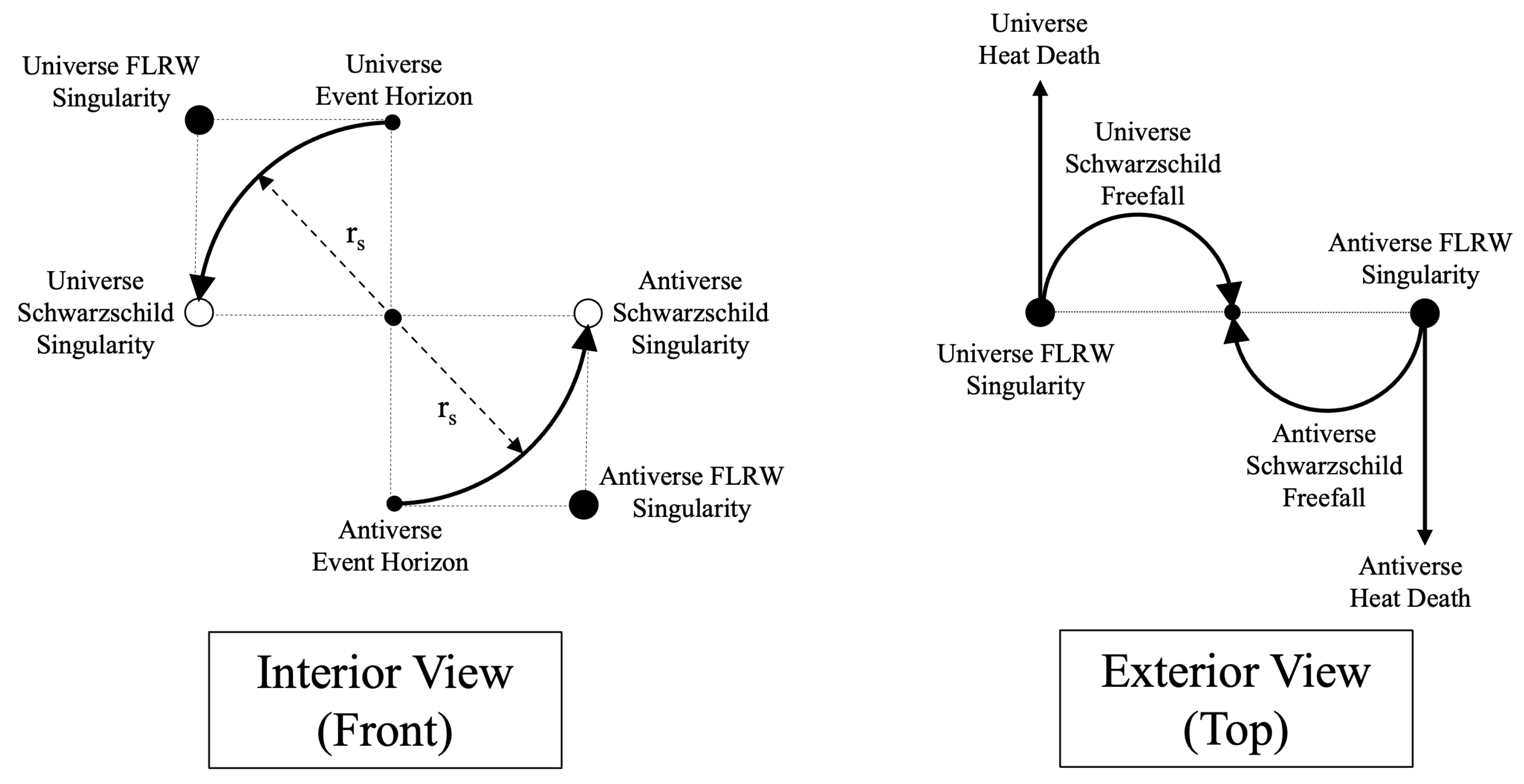
Let us break down Figure 2. First, we will refer to the second branch of the Schwarzschild and FLRW metrics on the Kruskal-Szekeres coordinate chart as the ’Anitverse’ to distinguish it from the Universe. On the left side of Figure 2, we see the curvature of the interior manifold. This Interior View is like looking at the $t=0$ lines in regions II and IV of Figure 1 on a plane perpendicular to the page at $X=0$.

The upper left arc represents region II in Figure 1 and the lower right arc represents region IV. The top and bottom dots at the center of the Interior View represent a point on the event horizon of the black hole in the Universe and Antiverse. The points on the left and right at the center of the Interior View represent the Schwarzschild singularities. The points in the top left and bottom right of the Interior View are the Big Bang singularities of the Universe and Antiverse. This view illustrates how the singularities can overlap on the Kruskal-Szekeres coordinate chart without actually intersecting in spacetime.

Looking at the Exterior View on the right side of the diagram, we are now looking at a ’top-down’ representation of the manifold containing the Big Bang singularities and event horizons. The three points in this view represent the same FLRW singularities and event horizons depicted in the interior view; we are just looking at them on the manifold that is oriented 90 degrees relative to the interior manifold.

So there are examples of two worldlines exiting the FLRW singularities in the Exterior View. The straight worldline represents the worldline of particles that never fall into a black hole and escape to infinity or the ’heat death’ of the Universe. The curved line represents the path of a particle that falls into a black hole. So, the way to look at this is to follow the curved line from the FLRW singularity to the center point of the Exterior View diagram which represents the event horizon. At that point, we move to the Interior View where the particle is at the top of the diagram for particles from the Universe and at the bottom of the diagram for particles from the Antiverse. These particles then fall to their respective singularities on the left and right sides of the view.

But these diagrams are practically screaming out to be completed. In particular, when we look at the interior view, one cannot help but feel like the circle needs to be completed. The circle can also be completed if we include time-reversed scenarios. Time-reversing the process involves swapping the functions of the singularities. In the time-forward case, the FLRW singularity is a source and the Schwarzschild singularity is a sink. In the time-reversed case, the FLRW singularity is a sink, and the Scbhwarzschild singularity is a source.

In the time-reversed case of the Interior View, matter would emerge from the singularity and move to exit the event horizon. In the time-reversed case of the Exterior View, particles would emerge from white holes and move toward the FLRW singularity as the Universe collapses.

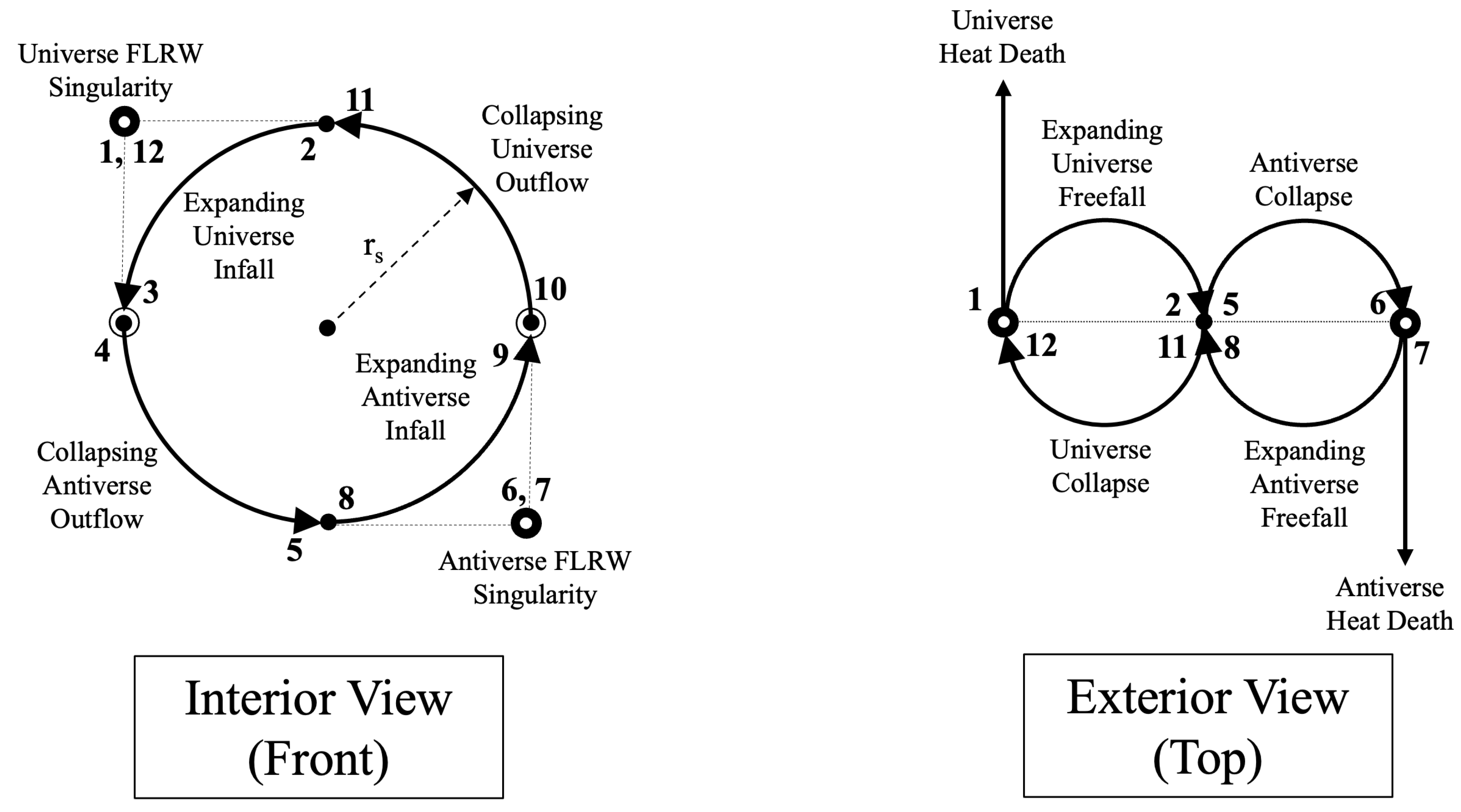
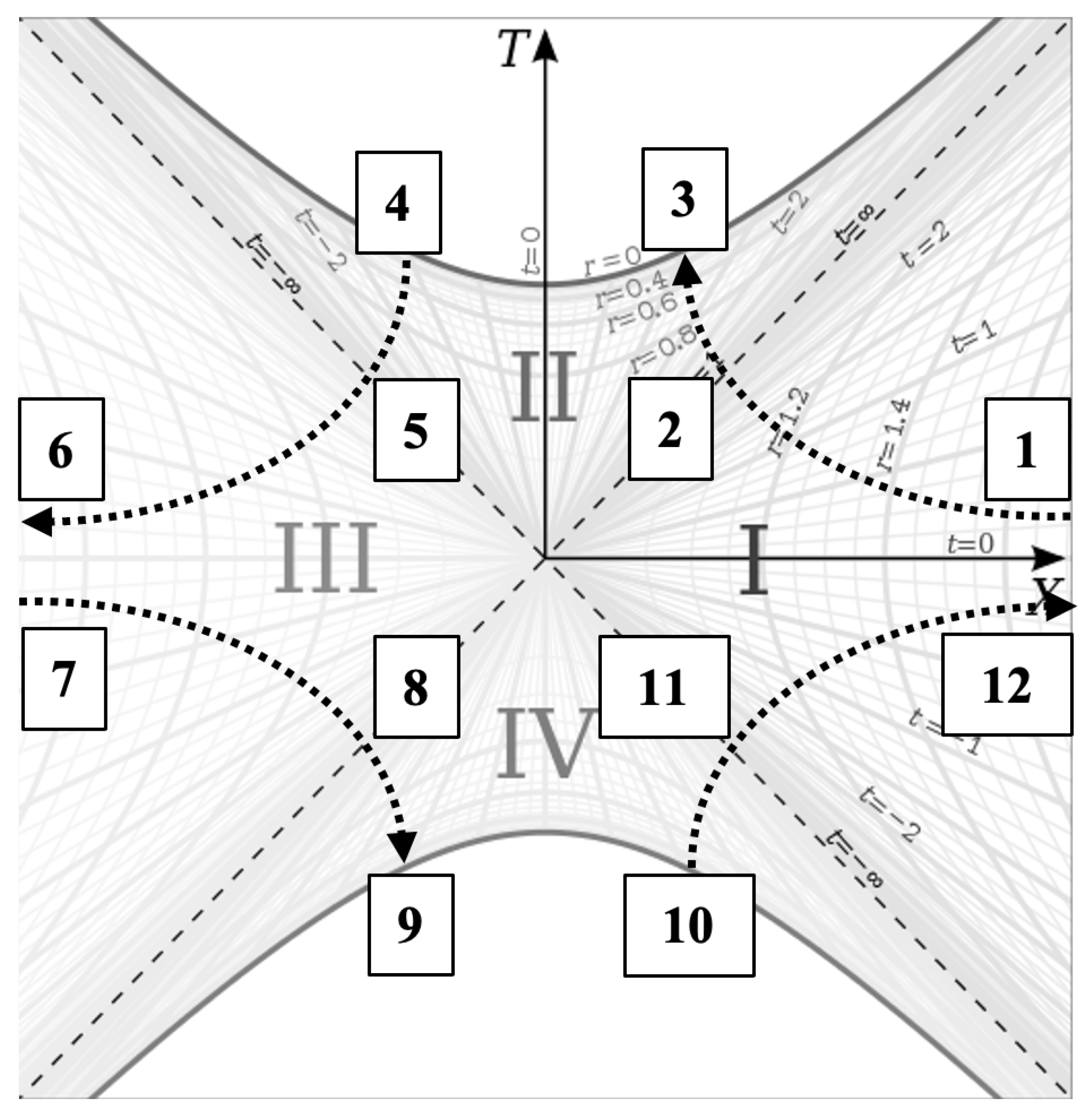
So, let us add the time-reversed worldlines to Figure 2 and interpret the results. Figure 3 adds the time-reversed processes with labels describing each process and numbers labeling important junctions.

Let us go through the process step-by-step starting at step 1, which is a particle leaving the Big Bang:

• Particle emerges from the Big Bang in the expanding Universe
• Particle crosses the event horizon in the expanding Universe at $t=\infty$
• Particle reaches the Schwarzschild singularity of the interior spacetime of the expanding Universe
• Particle emerges from the Schwarzschild singularity of the interior spacetime of the collapsing Antiverse
• Particle emerges from the white hole in the collapsing Antiverse at $t=-\infty$
• Particle reaches the Big Bang singularity of the collapsed Antiverse
• Particle emerges from the Big Bang in the expanding Antiverse
• Particle crosses the event horizon in the expanding Antiverse at $t=\infty$
• Particle reaches the Schwarzschild singularity of the interior spacetime of the expanding Antiverse
• Particle emerges from the Schwarzschild singularity of the collapsing Universe
• Particle emerges from the white hole in the collapsing Universe at $t=-\infty$
• Particle reaches the Big Bang singularity in the collapsed Universe
• Cycle begins again

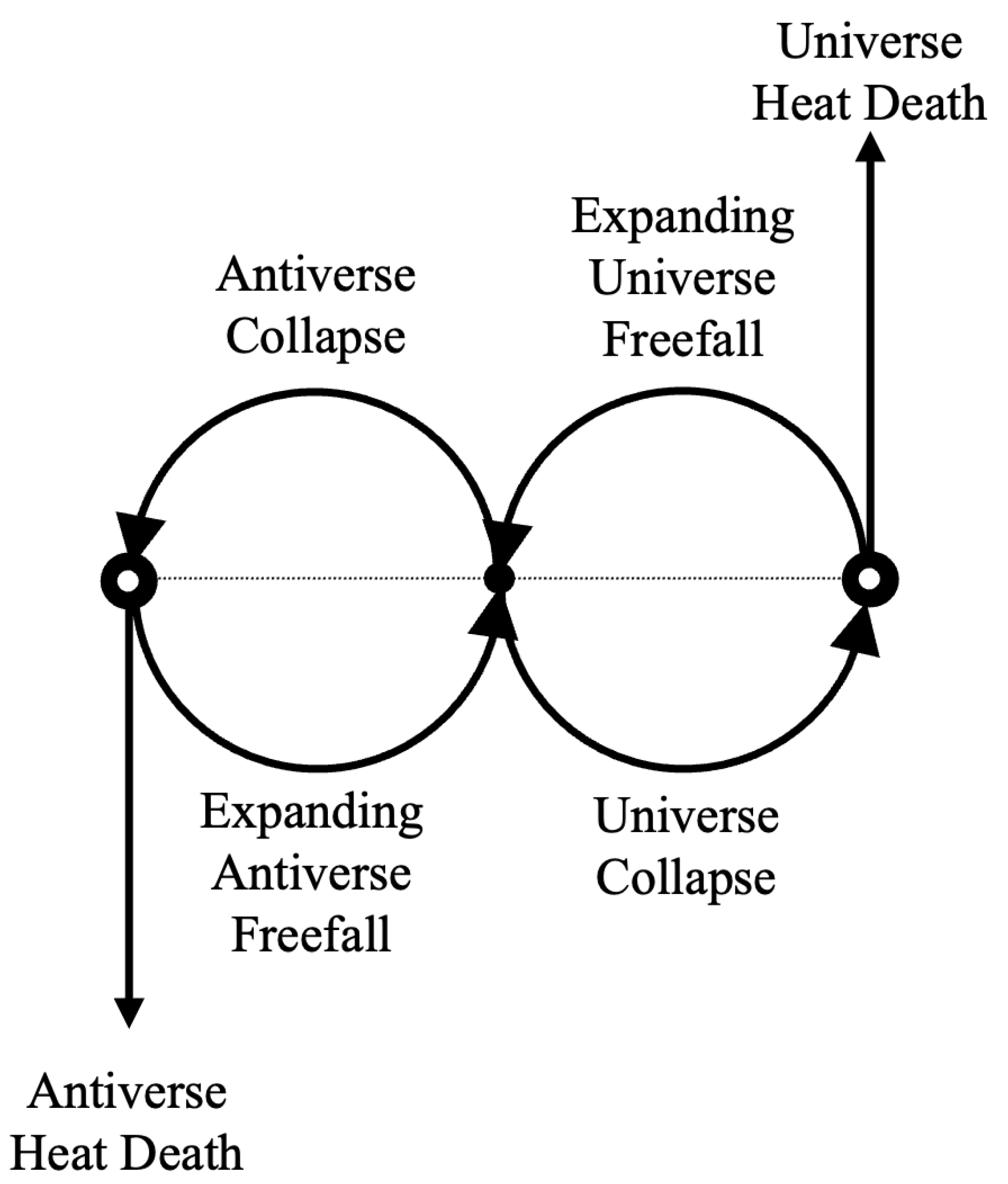
There is an obvious asymmetry in Figure 3. The expanding and collapsing exterior Universes sit in the top left quadrant of the full model, and the expanding and collapsing Antiverses sit in the bottom right quadrant; however, the other two quadrants are empty. This can be made symmetric by adding a second set of 4 spacetimes (Expanding Universe and Antiverse, collapsing Universe and Antiverse) but with their parity flipped relative to the original four spacetimes. So, the expanding Universe and collapsing Universe with flipped parity would be in the top right quadrant, with the heat death vector pointing up on the right side of the Exterior View of Figure 3. The expanding Antiverse and collapsing Antiverse with flipped parity would likewise go in the bottom left quadrant. The parity-flipped Exterior View is shown in Figure 4 below.

We can also map this whole process on the Kruskal-Szekeres coordinate chart in Figure 5 below.

In these diagrams, we place the FLRW singularities at infinity at $t=0$ and the same numbers used to enumerate the cycle in Figure 3 are labeled in this figure.

4. Freefall in the Schwarzschild Metric and Entropy Generation at the Singularity

In the previous section, we proposed a mapping of the path of freefalling particles through the singularities and expanding and collapsing Universes and Antiverses. We will now look at the worldlines of particles in the Schwarzschild spacetime to understand better the nature of the worldlines inside the black/white holes and at the singularity.

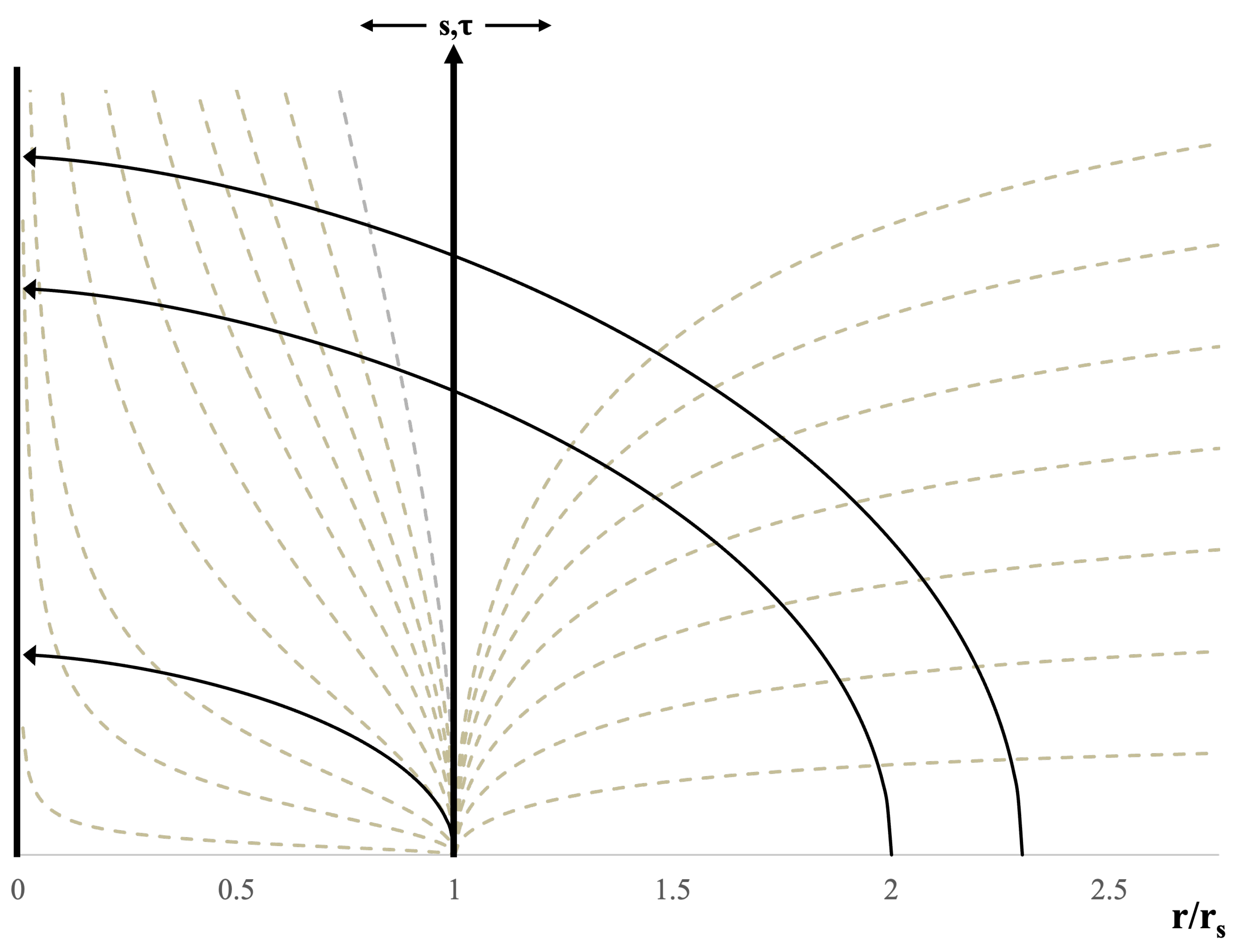
For this we will construct a new coordinate chart for the Schwarzschild metric. In this chart, use the proper interval as the vertical axis and the radius as the horizontal axis.

We first examine the exterior manifold on this chart. The t coordinate is the time coordinate here, so on this chart, we want surfaces of constant t. At fixed r, points on each of the lines of constant t are found by setting $dr=0$ in equation 5 to get $d\tau =\sqrt{1-{\displaystyle \frac{r_s}{r}}}dt$. When integrating, this gives $\tau =t\sqrt{1-{\displaystyle \frac{r_s}{r}}}$. So if we plot $\tau$ vs. r for different fixed values of t, we get a set of curves represnting foliations of constant t of the extrior manifold.

We do the same for the interior metric; only this time, instead of using the proper time, we need to use proper distance: $ds=\sqrt{{\displaystyle \frac{r_s}{r}}-1}dt$ and integrating gives us $s=t\sqrt{{\displaystyle \frac{r_s}{r}}-1}$. And we then plot lines of constant t using this equation. Figure 6 shows this coordinate chart with three different worldlines falling from rest at $t=0$ for different values of r.

To create the freefalling worldlines, we need to find the expression for proper time as a function of r for the freefaller. We start with the per-unit-mass energy condition:

$$E^2={\left({\displaystyle \frac{dr}{d\tau }}\right)}^2+\left(1-{\displaystyle \frac{r_s}{r}}\right)$$

(24)

The particle falls from rest at $r_0$, meaning ${\displaystyle \frac{dr}{d\tau }}=0$ at $r_0$. Therefore $E=\sqrt{1-{\displaystyle \frac{r_s}{r_0}}}$. This gives us the following expression for a particle falling from rest at $r_0$:

$${\displaystyle \frac{dr}{d\tau }}=-\sqrt{r_s\left({\displaystyle \frac{1}{r}}-{\displaystyle \frac{1}{r_0}}\right)}$$

(25)

Integrating this expression gives us the desired function:

$$\tau =\sqrt{{\displaystyle \frac{r_0^3}{r_s}}}\left[{cos}^{-1}\left(\sqrt{{\displaystyle \frac{r}{r_0}}}\right)+\sqrt{{\displaystyle \frac{r}{r_0}}}\sqrt{1-{\displaystyle \frac{r}{r_0}}}\right]$$

(26)

Equation 26 is the equation used to plot the solid lines on Figure 6 which represent particle falling from $r=r_s$, $r=2r_s$, and $r=2.3r_s$.

We typically think of the coordinates switching roles when the particle crosses the horizon such that the r coordinate becomes the time coordinate in the interior metric. But there is another way to interpret this. We can look at it as the particle’s worldline becoming spacelike at the horizon. The spacelike worldline has to keep moving through space, it cannot slow down. This is why the particles are driven toward the singularity, they cannot come to rest in the interior metric because they are spacelike. This explains why the proper interval on Figure 6 is the proper distance and not proper time for $r<r_s$. Proper distance is the interval we use to measure spacelike worldlines.

If we compare the worldline at the singularity to the worldline when the particle was at rest, we note that when the particle is at rest, the worldline is parallel to the proper time interval axis. However, at the singularity, the worldline is perpendicular to that axis.

The infalling speed of light in the exterior metric at some $r_0$ is given by:

$${\left({\displaystyle \frac{dr}{dt}}\right)}_c=-\left(1-{\displaystyle \frac{r_s}{r_0}}\right)$$

(27)

If we express this in terms of proper time of the observer at rest (${\tau }_0$) at $r_0$ instead of t, we get the following:

$${\left({\displaystyle \frac{dr}{d{\tau }_0}}\right)}_c={\left({\displaystyle \frac{dr}{dt}}\right)}_c{\displaystyle \frac{dt}{d{\tau }_0}}=-{\displaystyle \frac{1-\frac{r_s}{r_0}}{\sqrt{1-\frac{r_s}{r_0}}}}=-\sqrt{1-{\displaystyle \frac{r_s}{r_0}}}$$

(28)

If we compare Equation 28 to Equation 25, we see that, at $r=r_s$ for an observer falling from $r_0$, their ${\displaystyle \frac{dr}{d\tau }}$ is equal to ${\left({\displaystyle \frac{dr}{d{\tau }_0}}\right)}_c$, which is the speed of light in the frame of a rest observer at the location from which they began falling. So, in the frame of the observer at rest at $r_0$, the falling observer is moving at the speed of light as they cross the horizon. In the frame of the rest observer, the freefaller reaches the speed of light at the horizon and then becomes spacelike as they cross it until the falling worldline becomes horizontal on the coordinate chart at the singularity. The particle essentially has infinite velocity relative to the observer at rest when it reaches the singularity.

Note that in Figure 6, we have only used positive t on the chart. We can account for negative t by mirroring the chart in the $r=0$ line, which essentially gives us the top left quadrant of the Kruskal Szekeres chart, where we said the particles emerge from a white hole into a collapsing spacetime. Doing this gives the worldline a way to transit the singularity.

So relative to the rest observer, the freefalling worldline starts to go backward in time (the worldline goes from being horizontal on the chart to moving in a downward direction). This is why we say that the particle emerges into the Antiverse. It is the Antiverse because, in the Antiverse, particles move through time in the opposite direction relative to particles in the Universe. This also suggests that the particles in the Antiverse are antiparticles if the particles in the Universe are particles.

Now, for both the freefalling particle and infalling light, ${\displaystyle \frac{dt}{dr}}$ goes to zero at the singularity. For the freefalling particle, this does not mean it stops at the singularity. We note that as the worldline approaches the singularity, $dt$ is negative because the line starts at $t=\infty$ at the horizon and moves to $t=0$ at the singularity. But in the mirrored spacetime, the worldline emerges from the singularity at $t=0$ and moves toward $t=-\infty$ at the white hole horizon, meaning $dt$ is also negative in that case. Furthermore, $dr$ is negative when approaching the singularity and positive when leaving the singularity. Therefore, ${\displaystyle \frac{dt}{dr}}$ is positive when approaching the singularity and negative when leaving the singularity, which is why it is zero at the singularity. Therefore, the particle can transit the singularity.

But radially infalling light is infitiely redshifted as it approaches the singularity and any light emitted from the singularity is also infinitely redshifted. Therefore, radially infalling light effectively cannot pass the singularity. This might seem like a paradox, expect that, as has been argued, the particle’s worldline is spacelike and therefore it is as though the speed of the radially falling light is zero in the frame of the particle at the singularity. At that point, the particle is effectively moving so fast that light itself cannot follow. In other words, observers looking into the white hole from the collapsing Anitverse cannot see the light that fell into the black hole in the expanding Universe.

We also see that at $r=0$, the worldlines for particles that fell from different values of $r_0$ are separated by a finite proper distance, they are not infinitely stretched. So if the $r_0=2r_s$ and $r_0=2.3r_s$ worldlines represented the worldlines of the feet and head of an observer falling to the singularity, we see that the proper distance between the feet and head at the singularity is finite and therefore the observer is not infinitely stretched.

However, the angular dimensions do collapse at the singularity such that the observer will be squeezed infinitely in the angular dimensions there. Thus, any structure falling to the singularity will be destroyed by this crush, and the information will be scrambled at the singularity. Particles may even emerge from the singularity in both directions after this crush, where particles emitted into the negative t space will escape out of the white hole into the collapsing Antiverse as high entropy matter while any particles emitted into the positive t space would either fall back to the singularity or be emitted from the black hole back into the expanding Universe as spacelike particles.

We can therefore imagine that the singularity is surrounded by a hot, chaotic region of particles falling in and popping out. If spacelike particles can, in fact, be re-emitted into the expanding Universe, they could be candidates for Dark Matter, appearing as particle-sized event horizons. The Dark Matter in this scenario would be like smoke generated by the gravitational singularities. This is obviously highly speculative at this stage and would require further research to model such a system.

Therefore, we have shown that massive particles can in fact transit the Schwarzschild singularity, but any information associated with the particles is destroyed when reaching it and the entropy of the particles leaving the white hole will be maximized.

We can revolve Figure 6 about the $r=0$ axis to show the $\varphi$ dimension as well. Interestingly, we have two choices for how we revolve the spacetime for the $\varphi$ dimension. We can revolve it clockwise or counter-clockwise. This rotational choice changes the parity of the spacetime (a given angular velocity is positive in one case and negative in the other). What is notable is that the two configurations are superposed on one another and they share the same singularity.

5. Transiting the FLRW Singularity

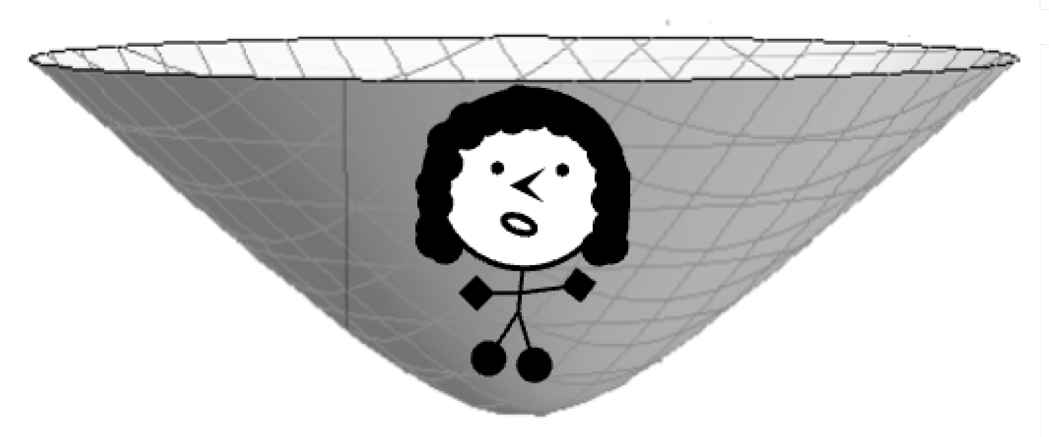
We began this paper by expressing the FLRW metric in Kruskal-Szekeres coordinates and found that the FLRW singularity is a hyperbola on the Kruskal-Szekeres coordinate chart at $T=1$. Let us depict an observer, Scout, on a spacelike surface in the FLRW metric at some time t swept around the $\varphi$ axis in Figure 7 below.

The surface in this case is a 2-sheeted hyperboloid that is homogeneous, isotropic, and spherically symmetric. The circles on this surface represent the r FLRW coordinate. We can change the center point $r=0$ on the surface by hyperbolically rotating the surface. Note that there is also a choice of parity with this surface where we can create it by revolving clockwise or counter-clockwise, and both situations are superposed.

But the FLRW singularity is an infinite volume (the surface in Figure 7 shows the singularity, and we can see that we can place each point of Scout’s body at a different point on the surface). What makes this particular surface special is that all points on the surface are connected by null geodesics (per Equation 20). Thus, at the instant of the singularity, all points in the infinite space can exchange information instantaneously. Therefore, the singularity represents a kind of initial condition where the exact state of the Universe at that time is completely defined and known everywhere in space.

Recall that the FLRW Big Bang is preceded by a collapsing Universe. In the collapsing Universe and Antiverse, gravity would become repulsiveblack holes cannot form in the negative t sections of regions I and III of the Kruskal Szekeres chart). So, in the collapsing Universe/Antiverse, matter is ejected from white holes scattered throughout infinite space, and these particles will gravitationally repel each other as they come close to one another. If, for this thought experiment, we ignore all other forces, then this situation will result in particles being evenly spread out, and it will get hotter and hotter over time since the particles are all continuously bouncing off each other and the space is also collapsing (collapsing space can be equivalently described as light requiring less time to move between two comoving points over time. And since all speeds are relative to light speed, if it takes lees time for light to travel between two points, it will also take everything else less time to travel, all other things being equal). So, by the end of the collapse, when the particles enter the Big Bang, depicted in Figure 7, the particles do not occupy the same location; rather, they are evenly spread over the surface and very hot, which are the conditions we associate with the Big Bang.

Furthermore, this Big Bang condition is an exact microstate of the Universe (i.e., the maximum knowledge of the positions and velocities of every particle that can be known is known at all locations), and therefore, the entropy of the Universe is at a minimum here. It’s as though the exact state of the entire Universe is measured there and then evolves from that point forward.

6. The Paradox of Infinite Time

Let us now consider the ’Heat Death’ path of the Universe. It is assumed that particles that follow a Heat Death path of the Universe will simply expand in the Universe forever; from one perspective, this may be what occurs. But let’s consider what happens at $t=\infty$ for an observer in the FLKRW metric looking at a black hole into which our brave explorer Scout is falling.

This observer would never have seen Scout fall into the black hole before this point. In fact, the observer wouldn’t have seen anything fall into the black hole (or even see the black hole form in the first place) up to this point, because, from this perspective, Scout and everything else reach the horizon at $t=\infty$. Therefore, the outside observer will not see them reach the horizon until $t=\infty$. But let’s just assume that there is an observer at $t=\infty$ looking at the black hole. What would they see?

What if we assume that $t=\infty$ and $t=-\infty$ intersect in the FLRW spacetime? That would mean that at $t=\infty$, the black hole event horizon in the expanding Universe would become the white hole event horizon in the collapsing Universe. So, after infinite time, the heat death observer would finally see Scout completely disappear at the horizon (because her radiation would be completely redshifted), and at that moment, they would see maximum entropy matter emerging from the horizon. This would be the particles that fell into the black hole in the expanding Antiverse, were converted to high entropy particles at the singularity, and are now coming out of the white hole. Based on what has been found in this paper, this would mean the Heat Death observer would also see the Universe begin to collapse at this time (because they would now be in what we have labeled the collapsing Universe).

Furthermore, if we assume that the Antiverse is exactly identical to the Universe with the only difference being that matter is exchanged for antimatter, then the particles that the heat death observer sees coming from the white hole would effectively be the same particles that they saw falling toward the horizon, just reconfigured with maximum entropy.

The observer would see Scout and all the infalling matter shatter like fine glass against the phantom surface, with the scrambled wreckage pouring down into the collapsing Universe. What they witness in that moment is the intersection of infinities.

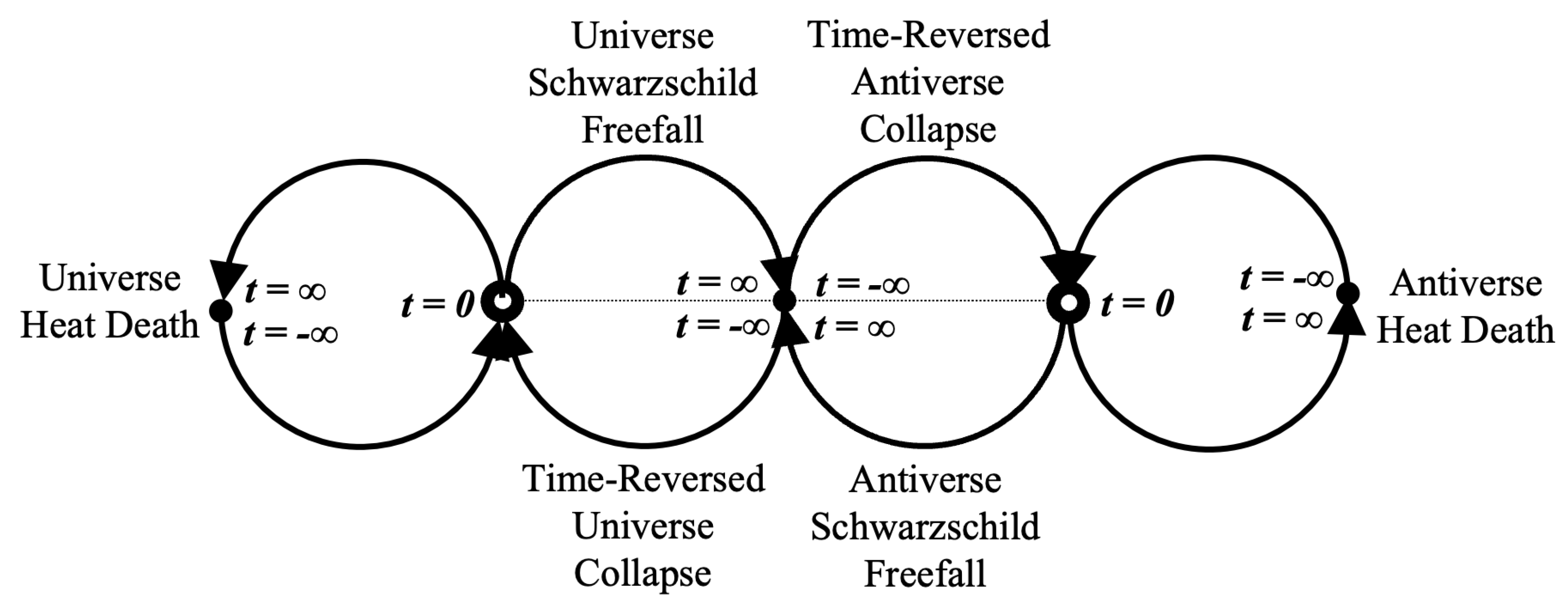
This also allows us to complete the symmetry of Figure 3 by adding the intersection of $t=\infty$ and $t=-\infty$ to the diagram at Heat Death. Figure 8 shows the updated diagram with the values of time t marked at the relevant locations. The new lobes on each side of the diagram are like stereographic projections of a line centered at the Big Bang extending to positive infinity in one direction (say, up in the diagram) and negative infinity in the opposite direction with the Heat Death point acting as the ’north pole’ of the projection.

Without some additional mechanism, no conscious observers could actually reach the Heat Death point, because that would require infinite proper time. Such a mechanism might be a rotating cosmology or something else, such as a charged cosmology. These properties may even lead to an explanation for the Dark Energy observations.

But for fundamental particles, perhaps infinite time is not a concern with regard to this model. It is notable, nonetheless, that particles taking the black/white hole route will experience a finite proper time from one Big Bang to the next.

7. Conclusion

We have presented a model of reality in which worldlines cycle endlessly between an expanding Universe and Antiverse, as well as their collapsing counterparts. The Schwarzschild black holes act as engines, shuttling particles between these universes and converting matter into antimatter and vice versa in the process.

The Schwarzschild singularity is a time when maximum entropy is generated, whereas the Big Bang singularity is a time when entropy is minimized. In order to complete the symmetry of the model, it is necessary to assume that the FLRW $t=\infty$ and $t=-\infty$ times intersect at heat death. The model provides an eternal view of reality, with no beginning or end. It does, however, suggest that different initial conditions can exist at the Big Bang of each cycle, providing infinite possible configurations of reality that follow the rules of this model.

Imagine the particles inside the black hole as a group of dice cupped and shielded in the palms of a seasoned gambler. They are thoroughly shaken at the Schwarzschild singularity and then thrown down from the white hole. After tumbling through the collapsing spacetime, they land in an exact state on the FLRW singularity, and the next turn of the game unfolds according to that outcome.

We only considered non-rotating black holes in this analysis; however, for the more realistic case of rotating black holes, the ring singularity may alter the experience of falling through the center of the black/white hole. We can surmise, however, that just as the Universe has rotating black holes, this implies that the collapsing Universe must have rotating white holes. A more thorough investigation of the rotating black hole scenario will be left for future research.