Revisiting the Anisotropy of the Schwarzschild Metric

I. Introduction

The Schwarzschild metric describes two spacetimes separated by an event horizon. The spacetime outside this horizon is well understood and its predictions have been successfully verified over the past century. The spacetime inside the horizon, commonly treated as the spacetime inside a black hole, has been believed to be unobservable to anyone outside of a black hole since light is not able to cross from inside to outside the horizon. As such, it is believed that the predictions associated with this spacetime are untestable.

The Schwarzschild coordinates are useful when examining this metric because in the exterior metric, the r coordinate represents a spacelike radius and the t coordinate is the timelike coordinate and the azimuthal coordinate represented by $\Omega$ is a unit 2-sphere. When moving from the exterior region to the interior, the signs of the r and t coordinate flip such that the r coordinate is now timelike and the t coordinate is spacelike.

In this paper, we examine the isotropy of the interior metric and its relationship to Kantowski-Sachs metrics and find that the azimuthal scale factor is not describing the collapse of two out of three dimensions of space to a point, but rather the azimuthal term of the interior metric causes an inertial acceleration of reference frames moving on curved paths that becomes infinite at the singularity. This acceleration is shown to be caused by the ’spin’ of space around the observer’s reference frame, resulting in the angular acceleration of the observer.

The re-interpretation of the meaning of the azimuthal term of the interior metric as well as an understanding of the $dt$ term of the metric as a hyperbolic angle leads to the conclusion that while the exterior metric may be anisotropic, the interior metric is spatially isotropic and homogeneous at a given r. This result could have major implications for Cosmology as it demonstrates that the interior Schwarzschild metric is in fact isotropic and homogeneous, properties shared by the cosmic voids in the Universe.

II. Comparison of the Exterior and Interior Metrics

The Schwarzschild metric has the following form:

$$d{\tau }^2=-\left({\displaystyle \frac{u}{r}}-1\right)d{t}^2+{\displaystyle \frac{1}{\frac{u}{r}-1}}d{r}^2-r^{2}d{\Omega }^2$$

(1)

The exterior metric, which describes the spacetime around a spherically symmetric mass is given for values of $r>u$ where u is the Schwarzschild radius $r_s$ related to the mass M of the source given by $r_s=2GM$. This metric treats the mass of the source as being concentrated at point at the center of the spacetime.

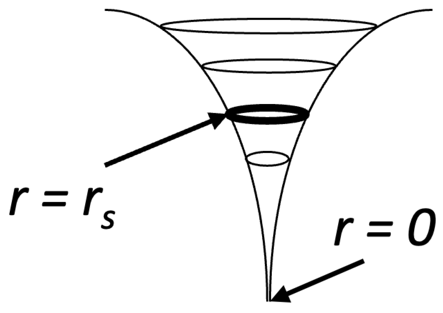
The interior metric is known as a ’Kantowski-Sachs’ spacetime [1] which has different linear and azimuthal scale factors. This is understood to mean that the spacetime is anisotropic. Figure 1 shows a common depiction of the gravitational well of the Schwarzschild metric ($dt=d\theta =0$, $\theta ={\displaystyle \frac{\pi }{2}}$).

We are given the impression here that the geometry inside and outside the event horizon are the same with the main difference being that once an observer crosses the event horizon ($r=r_s$), they will continue to fall to the singularity at $r=0$ where they will be ’spaghettified’ as a result of the radius of the 2-sphere collapsing to a point and the t dimension becoming infinitely stretched.

However, we must be careful with the sign changes in the metric as the horizon is crossed. In the common interpretation, the azimuthal term is interpreted the same outside and inside the event horizon even though the radius goes from being spacelike to being timelike. In the exterior metric, $rd\varphi$ is an arc length, but in the interior metric, it is a time (because r has units of time). And if we treat r as simply a scale factor, then it is scaling the angles themselves, not the arc length. Furthermore, if the radius is a time, then it is unclear what it would mean to revolve around a future point in time ($r=0$).

So we need to examine the exterior and interior geometries more closely to understand how exactly they are different, particularly in regards to the meaning of the azimuthal term in each case. The Kruskal-Szekeres coordinates are very useful for this task. As we will see, the Kruskal-Szekeres coordinate chart allows us to see how the t and r coordinates are curved relative to Minkowski space. But first, we define the Kruskal-Szekeres coordinates in terms of the Schwarzschild coordinates. For the exterior metric:

$$\begin{array}{c}\hfill T=\sqrt{\left({\displaystyle \frac{r}{r_s}}-1\right)e^{{\displaystyle \frac{r}{r_s}}}}sinh\left({\displaystyle \frac{t}{2r_s}}\right)\\ \hfill X=\sqrt{\left({\displaystyle \frac{r}{r_s}}-1\right)e^{{\displaystyle \frac{r}{r_s}}}}cosh\left({\displaystyle \frac{t}{2r_s}}\right)\end{array}$$

(2)

And for the interior metric:

$$\begin{array}{c}\hfill T=\sqrt{\left(1-{\displaystyle \frac{r}{u}}\right)e^{{\displaystyle \frac{r}{u}}}}cosh\left({\displaystyle \frac{t}{2u}}\right)\\ \hfill X=\sqrt{\left(1-{\displaystyle \frac{r}{u}}\right)e^{{\displaystyle \frac{r}{u}}}}sinh\left({\displaystyle \frac{t}{2u}}\right)\end{array}$$

(3)

With these definitions, we can plot the Kruskal-Szekeres coordinate chart [2]:

Figure 2. Kruskal-Szekeres Coordinate Chart

Figure 2. Kruskal-Szekeres Coordinate Chart

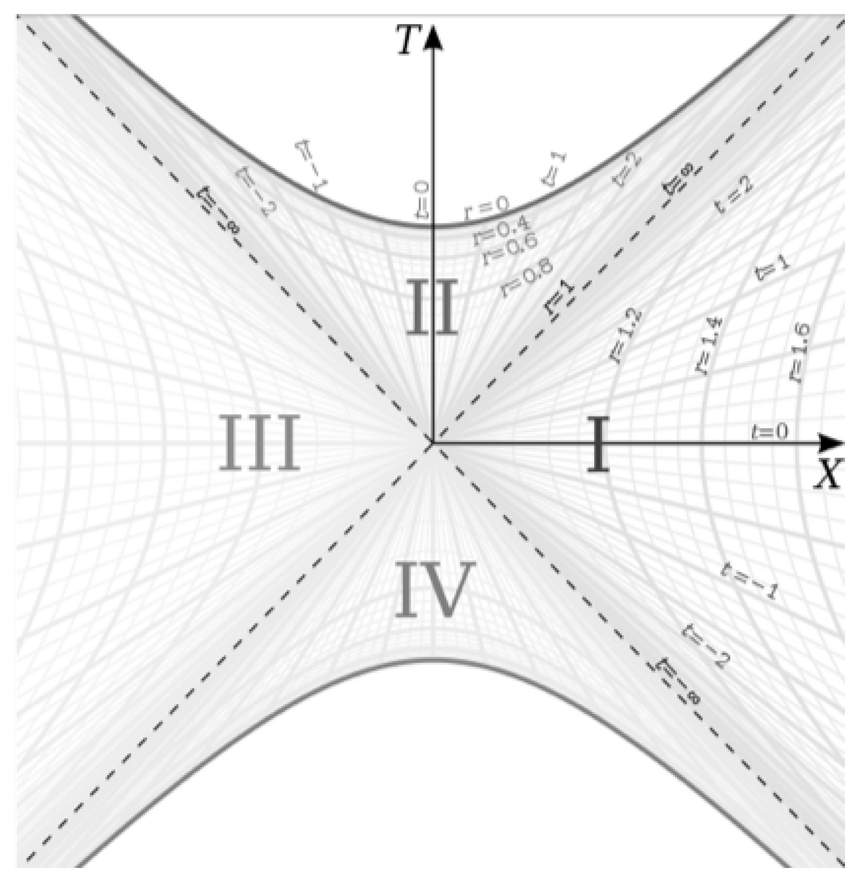
In this paper, we will focus on regions I and II of this chart, representing the exterior and interior metrics respectively. Since the Kruskal-Szekeres coordinates are defined in such a way that null geodesics are 45 degree lines everywhere on the chart and the T and X coordinates are straight and mutually perpendicular everywhere on the chart, we can think of the T-X grid as Minkowski space with the curved r and t coordinates overlaid on the grid. Thus, this chart clearly shows how the Schwarzschild space and time coordinates r and t are curved relative to the Minkowski coordinates T and X. We see that the r coordinate lines are hyperbolas, which captures that fact that an observer at rest in the exterior metric experiences a constant acceleration, and the t coordinate is a hyperbolic angle. That t is a hyperbolic angle will become an important fact when we look at the geometry of the interior metric.

We see from equations 2 and 3 that we need separate Kruskal-Szekeres coordinate definitions for the exterior and interior metrics, but we can combine these into a single relationship as follows

$$X^2-T^2=\left({\displaystyle \frac{r}{u}}-1\right)e^{{\displaystyle \frac{r}{u}}}$$

(4)

Equation 4 is applicable to both the interior and exterior solutions. For the exterior metric, $X^2-T^2>0$ and for the interior solution, $X^2-T^2<0$.

The equation for a 2D hyperboloid surface embedded in three dimensions is given by:

$${\displaystyle \frac{x^2}{a^2}}+{\displaystyle \frac{y^2}{b^2}}-{\displaystyle \frac{z^2}{c^2}}=\pm 1$$

(5)

For our purposes, we will be considering the special case where $a=b=c$, which gives the one and two sheeted hyperboloids of revolution. Equation 4 appears to be only for one dimension of space, but if we think of X as a radius, then it can describe 3 sphrically symmetric dimensions of space.

So comparing to Equation 5, if we set $a^2=b^2=c^2=\left({\displaystyle \frac{r}{u}}-1\right)e^{{\displaystyle \frac{r}{u}}}\equiv {\rho }^2$ and $X^2\equiv R^2=x^2+y^2$ where R is a radius of a circle in this example, we obtain an equation that matches the form of Equation 5 where :

$$R^2-T^2={\rho }^2$$

(6)

Equation 6 describes 2D hyperboloid surfaces for a given r where the interior metric has negative ${\rho }^2$ and the exterior metric has positive ${\rho }^2$. Let us now visualize a surface of constant r in both the exterior and interior metrics. For the exterior metric at some $r>r_s$, we get the following hyperbolid of revolution:

Figure 3. Surface of Constant $r>r_s$ for the Exterior Metric in Kruskal-Szekeres Coordinates

Figure 3. Surface of Constant $r>r_s$ for the Exterior Metric in Kruskal-Szekeres Coordinates

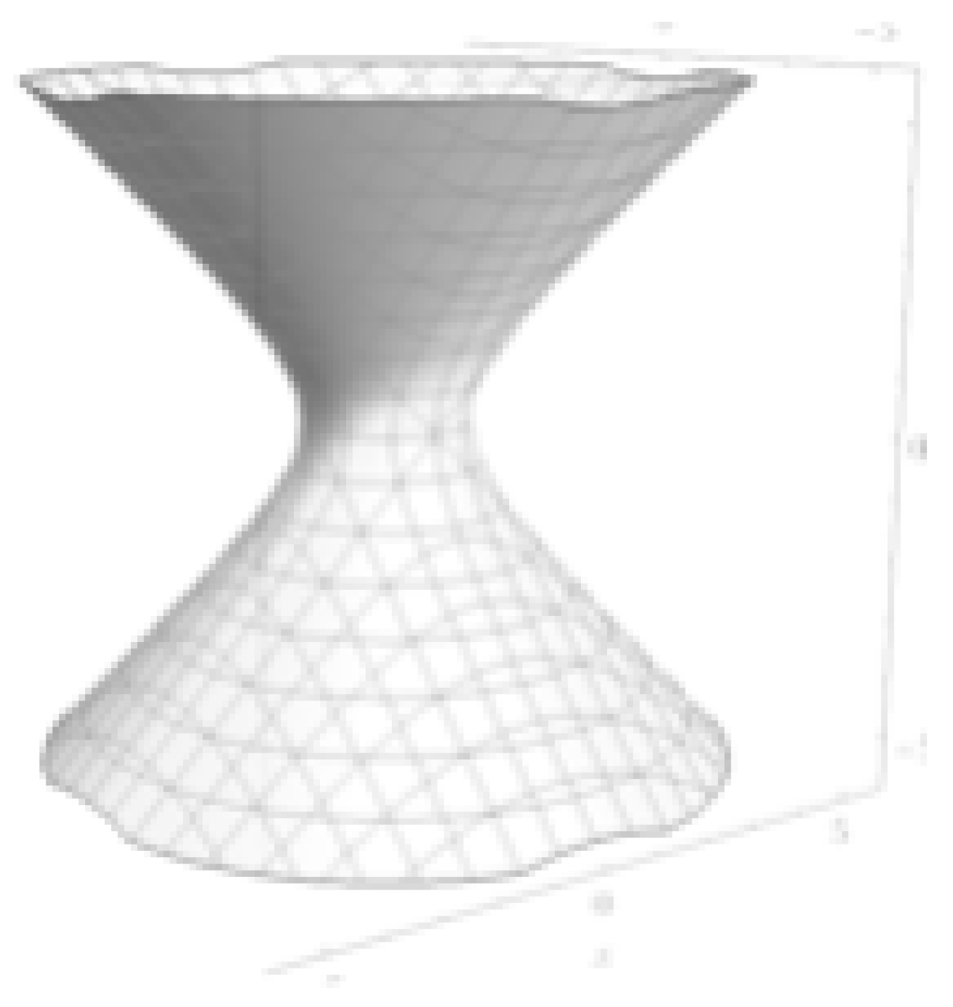
On this hyperboloid, the time coordinate t is marked as circles on the sheet and we have one free spatial coordinate $\varphi$ on the surface which is the angle of revolution of the surface. The $t=0$ location is at the throat of the hyperboloid. The first thing to note here is that the t coordinate can only be hyperbolically rotated in one direction: up or down. This is because the t coordinate is the coordinate of time and time only has one dimension so there can only be a hyperbolic rotation along the single time dimension. The second thing to notice is that the radius of the sheet is pointed perpendicular to the axis of circular rotation. This is why when a reference frame at some $r>r_s$ undergoes some angular rotation $d\varphi$, it moves along an arc length in space.

So we can see how if in Figure 3, r was timelike and t was spacelike, as is the case in the interior metric, then the spacetime would be anisotropic because in that case, the entire surface is spacelike and the spacetime looks different in different directions. In one direction, the space is closed (moving around a circle on the hyperbolid as r, which is the time coordinate in the internal metric, decreases), and in the perpendicular direction, the space is open (moving up or down on the hyperboloid).

So if a 2D foliation of the interior metric at some r was represented by the one-sheeted hyperboloid of revolution (like the exterior metric is), then the common visualization of the gravitational well in Figure 1 would be correct. However, we need to recall that for the interior metric, the right side of equation 4 is negative, which gives the following hyperboloid surface for some constant $0<r<u$:

Figure 4. Surface of Constant $0<r<u$ for the Interior Metric in Kruskal-Szekeres Coordinates

Figure 4. Surface of Constant $0<r<u$ for the Interior Metric in Kruskal-Szekeres Coordinates

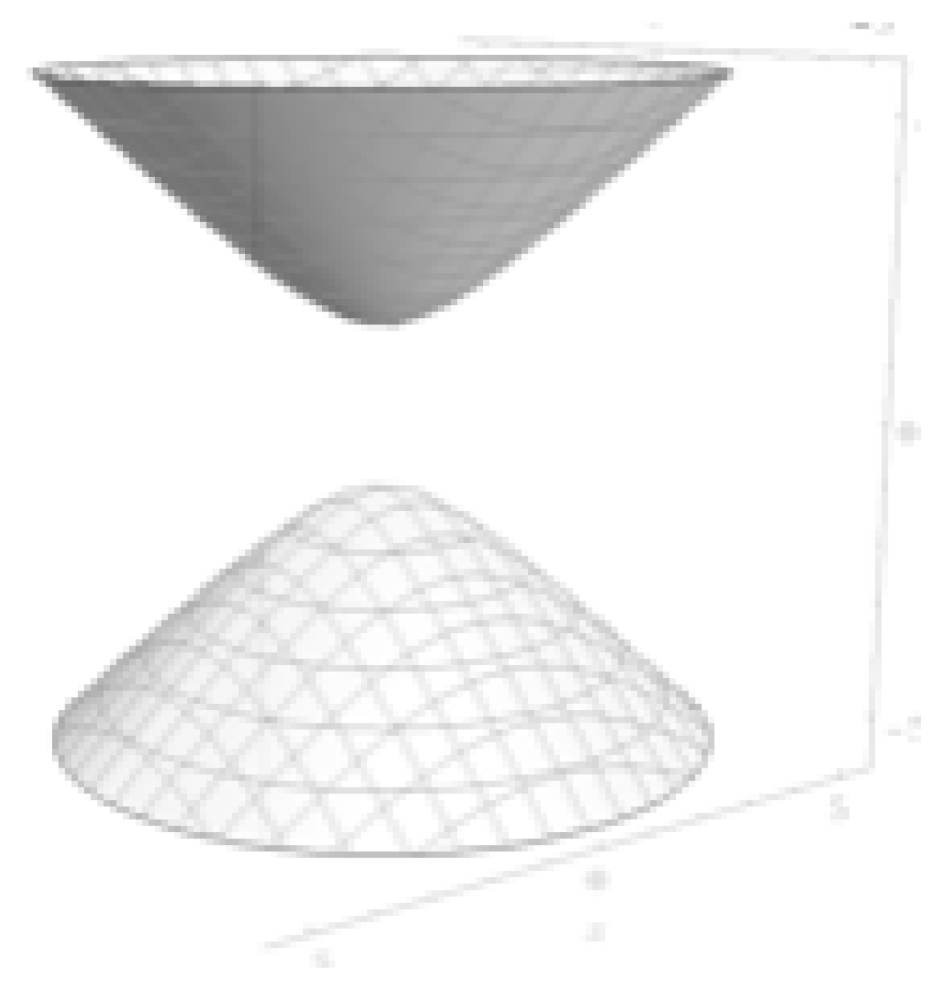
The first thing we notice is that this is a two-sheeted hyperboloid as opposed to the one-sheeted hyperboloid of the exterior metric. So right away, we can see that the interior and exterior geometries are different. In this paper, we will focus on the top sheet, representing a hyperbola in region II of Figure 2.

If we look at region II of Figure 2 in the context of Figure 4, we see that in contrast to the exterior metric where the radius perpendicular to the axis of circular rotation, in the interior metric, the radius is parallel to this axis. Recall that r is now the time coordinate and time is one dimensional, so the radial vector in this case is stuck in one dimension. Furthermore, we see that the t coordinate, which is a hyperbolic angle, can be rotated in 3 different dimensions now since the t coordinate is spacelike (we see two of the three dimensions in Figure 4). Since t is a hyperbolic rotation and ${\partial }_t$ is a Killing vector of the spacetime, we can hyperbolically rotate the space to move any point on the surface to $t=0$ which is at the apex of the hyperboloid. So just like we can set any arbitrary time as $t=0$ in the exterior metric, we can set any arbitrary location as $t=0$ in the interior metric. In particular, for a given reference frame we are examining, we can say that that reference frame is always at $t=0$, and when the frame moves in a particular direction, that is modelled as the hyperboloid being hyperbolically rotated in that direction such that the reference frame remains at $t=0$ as it moves.

Therefore, the t coordinate, which is a hyperbolic angle, is like a ’forward/backward’ coordinate. It represents the straight-line distance from the reference frame to some point. In the exterior metric, the hyperbolic rotation could only happen along one direction (the direction of time), but being spacelike in the interior metric, the hyperbolic rotation can now happen in any direction in three dimensions of space.

We can understand the nature of the t coordinate by imagining ourselves in the interior metric. The metric is an infinite dark vacuum so there are no reference points other than the frame itself, so the origin of space is always the reference frame itself, which is always $t=0$. So the velocity ${\displaystyle \frac{dt}{dr}}$ is always the velocity of the reference frame tangent to its worldline, regardless of whether the motion is in a straight line or curved. This is in contrast to the exterior metric where the velocity tangent to the worldline comes from a combination of radial velocity ${\displaystyle \frac{dr}{dt}}$ and tangential velocity perpendicular to the radius $r{\displaystyle \frac{d\Omega }{dt}}$.

This brings us to the azimuthal term of the interior metric. Consider Figure 5 which depicts an observer at point A moving to point B, stopping and then moving to point C (we are illustrating this on the lower hyperboloid, but the same applies to the upper hyperboloid.

Figure 5. Moving Between Points in the Interior Metric

Figure 5. Moving Between Points in the Interior Metric

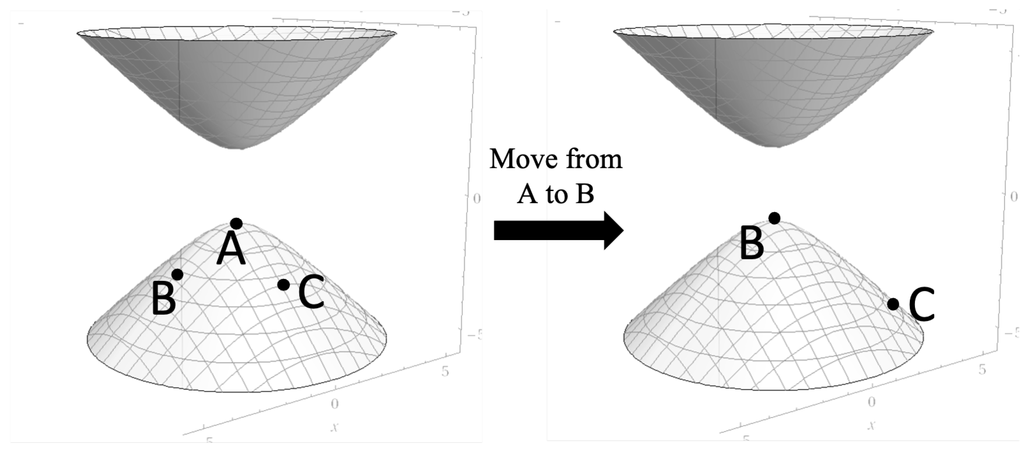
On the left half of Figure 5, we see the observer at point A. To go from A to B and then C, it looks like we would move along a hyperbola to get to B and then around the circle to get to C. But as is shown on the right side of Figure 5, as we move from A to B, we hyperbolically rotate the space along the direction AB. This hyperbolically rotates point B to $t=0$, A to the far side of the hyperboloid opposite to where B was on the left (so it is not visible in the diagram), and C moves along the hyperbola it was on in the same direction. And what we see here is that now to get from B to C, we do another hyperbolic rotation but in the direction BC on the right side of the diagram. So in taking the path AB, stopping, then BC, we see that there were only translations in t involved and nothing to do with the circular rotation $\varphi$.

So what then is the azimuthal term of the interior metric measuring? Let’s repeat the same motion in Figure 5 again, only this time we will move continuously from A to B to C without stopping. To do this, we would again apply a hyperbolic rotation from A to B and at the instant we reach B, we change the direction of the hyperbolic rotation to go from B to C. In this scenario, we are boosting the reference frame twice where the two boosts are not collinear. In Special Relativity, the application of non-collinear boosts like this causes the reference frame of the boosted observer to precess relative to the lab frame (in this case, the lab frame is the event horizon which for the interior metric is a shell surrounding the infinite space). If we consider continuous boosts, this effect is known as Thomas precession and is defined as [3]:

$${\overrightarrow{\omega }}_T={\displaystyle \frac{1}{c^2}}\left({\displaystyle \frac{{\gamma }^2}{\gamma +1}}\right)\overrightarrow{a}\times \overrightarrow{v}$$

(7)

Where

$$\gamma ={\displaystyle \frac{1}{\sqrt{1-\frac{v^2}{c^2}}}}$$

(8)

Where ${\omega }_T$ is the Thomas precession. Note that this precession doesn’t refer to any spatial center, it is determined entirely by the motion of the reference frame without reference to anything/anywhere external. The Thomas precession is like a ’spin’ of the reference frame which is essentially the precession of gyroscope attached to the reference frame relative to the surrounding shell. So if we put an arrow on the 2-sheeted hyperboloid of the internal metric at $t=0$ fixed and pointed in some arbitrary direction in space (representing the gyroscope of the reference frame), a change in the angle $phi$ of the metric corresponds to the hyperboloid rotating relative to that gyroscope.

We can now understand why in the interior metric, the radial vector is parallel to the axis of rotation as opposed to the exterior metric where the radial vector is perpendicular to the axis. In the interior metric, the azimuthal term is describing the rotation of space around the time dimension (r) of the reference frame and that rotation is known as the Thomas precession.

For the case of circular motion ($d\theta =0$, $\theta ={\displaystyle \frac{\pi }{2}}$), $\overrightarrow{a}\times \overrightarrow{v}=-av$ where a is the centripetal acceleration and $v={\displaystyle \frac{dt}{dr}}$, the tangential velocity. The centripetal acceleration can be expressed as $a=v\omega$ where $\omega$ is the angular velocity of the frame around the point at the center of the circular rotation. So $av=\omega {\left({\displaystyle \frac{dt}{dr}}\right)}^2$ and since ${\displaystyle \frac{dt}{dr}}$ is by definition the tangential velocity of the frame, ${\left({\displaystyle \frac{1}{c}}{\displaystyle \frac{dt}{dr}}\right)}^2=1-{\displaystyle \frac{1}{{\gamma }^2}}={\displaystyle \frac{(\gamma +1)(\gamma -1)}{{\gamma }^2}}$. If we substitute all this into equation 7, we get the following relationship for circular motion:

$${\overrightarrow{\omega }}_T=(1-\gamma )\omega$$

(9)

So for the case of circular motion, equation 9 allows us to relate the Thomas precession ${\omega }_T$ (i.e. the angular velocity in the interior metric) to the angular velocity $\omega$ of the frame.

The geodesic equation for angular motion [4] in the interior metric is given below (we will examine the case for planar rotation where $\theta ={\displaystyle \frac{\pi }{2}}$).

$${\displaystyle \frac{d^2\varphi }{d{\lambda }^2}}=-{\displaystyle \frac{2}{r}}{\displaystyle \frac{d\varphi }{d\lambda }}{\displaystyle \frac{dr}{d\lambda }}$$

(10)

If we choose $\lambda$ to be r in this analysis and assume an initial circular motion, we can integrate to get the angular velocity ${\omega }_T={\displaystyle \frac{d\varphi }{dr}}$ of the geodesic:

$${\omega }_T\left(r\right)={\omega }_{T,0}{\left({\displaystyle \frac{r_0}{r}}\right)}^2$$

(11)

Where ${\omega }_{T,0}$ is the initial precession. So the Thomas precession increases as r decreases (corresponding to time increasing) and becomes infinite at $r=0$, the singularity. Combining this with equation 9, we see that a frame in circular motion in the interior metric will have that circular motion accelerated over time as a result of the $\varphi$ geodesic equation.

This can be visualized better by looking at the worldline of a circular orbit in the exterior and interior metrics as shown in Figure 6:

Figure 6. Worldlines of Circular Orbits in the Exterior and Interior Metrics

Figure 6. Worldlines of Circular Orbits in the Exterior and Interior Metrics

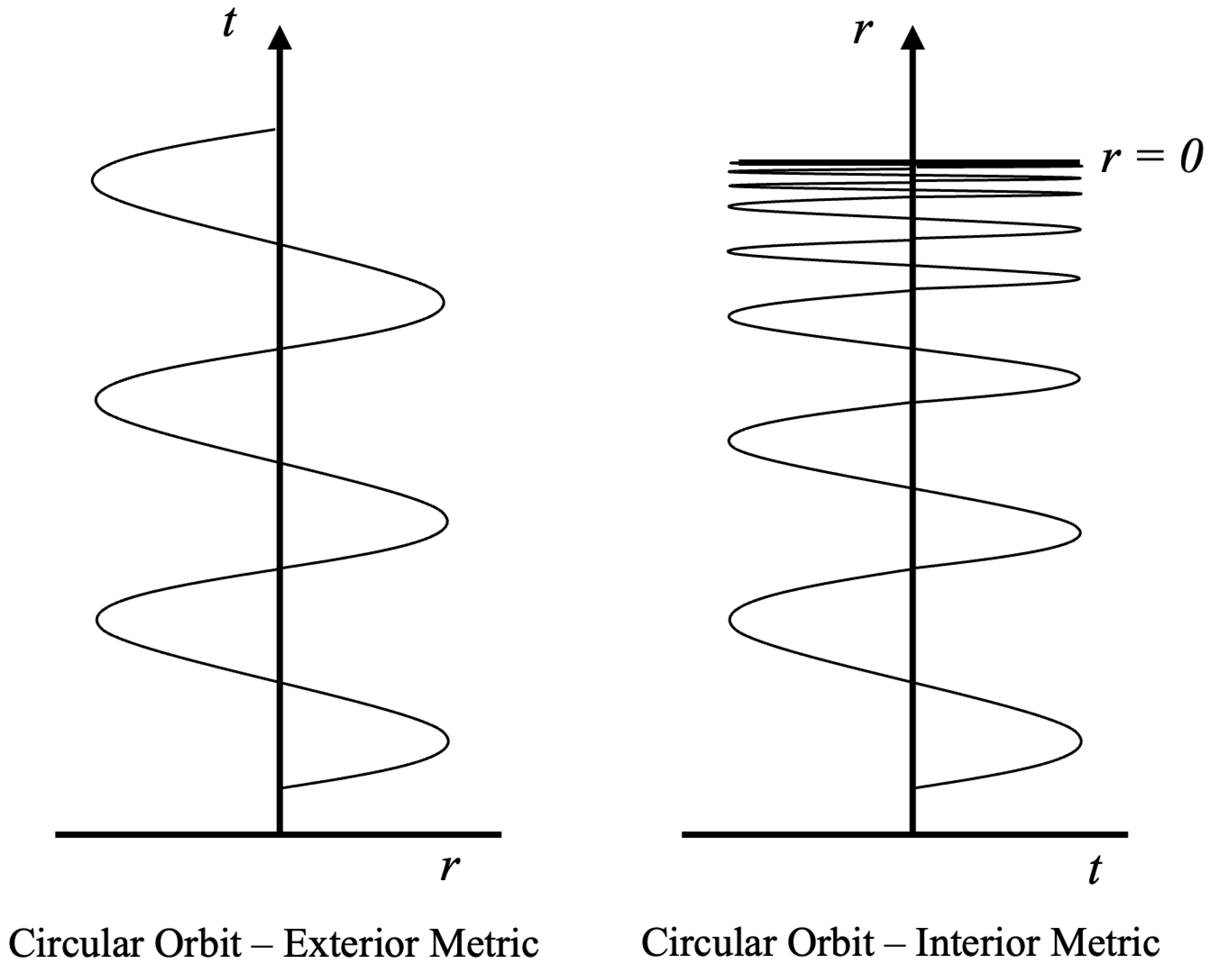
On the left side of the figure, we see the circular orbit ($dr=0$) in the exterior metric with time on the vertical axis and radius on the horizontal axis (a 2D projection of a 3D helix wrapped around the time axis). This a helix with constant radius r. The pitch of the helix is also a constant which means that the angular velocity of the worldline is constant over all time. Since the exterior metric is eternal, this helix can continue as shown for infinite t.

On the right side, we see the same circular orbit in the interior metric. First we note that the signature of the interior metric is flipped relative to the exterior metric and so the vertical time axis is now represented by the r coordinate and the horizontal space axis is represented by the t coordinate. Unlike in the exterior case, the interior metric is finite in time, so the worldline can not go beyond $r=0$. But we see that the pitch of the helix decreases to 0 as r goes to zero as though the infinite worldline from the exterior metric has been compressed to fit the finite time of the interior metric. A smaller pitch leads to an increasing angular velocity since it implies more rotations per unit time as r goes to zero.

So for any planar motion, $d\theta =0$ and $\theta ={\displaystyle \frac{\pi }{2}}$ in the interior metric. But the $\theta$ coordinate will come in to play if the observer moves on, say, a helical path through space (different from the helical path through spacetime depicted in Figure 6). On a planar, circular path, the observer would see the surrounding shell (if the shell were visible) spinning about an axis where the orientation of the axis remains fixed relative to the shell. On the helical path, the shell will be spinning around the observer, but the axis of the spin will change its orientation as the observer moves along the path and this is will introduce $\theta$ into the calculation.

So we have demonstrated that the interior metric is homogeneous and isotropic in space and that the azimuthal term of the metric is describing the Thomas precession of the moving frame. In the next section, we will reinforce the idea that the azimuthal term is describing the precession of gyroscopes relative to the surrounding shell by comparing this to the role of gyroscopes in the exterior metric’s azimuthal term.

III. Gyroscopes in the Exterior and Interior Metrics

Let us engage in a thought experiment involving the exterior metric where we consider an observer orbiting a Black Hole on a circular path in a tidally locked manner. For this experiment, we do not care about allowed orbits, we will assume a circular orbit at all times because we are investigating the underlying geometry of the space. We will also consider any geodedic precession as negligible for this thought experiment. The observer also has a gyroscope that was pointing directly at the center of the Black Hole when the orbit began. The orientation of the gyroscope at four different points in the orbit are shown in Figure 7 below.

Figure 7. A Gyroscope on a Circular Orbit Around a Black Hole

Figure 7. A Gyroscope on a Circular Orbit Around a Black Hole

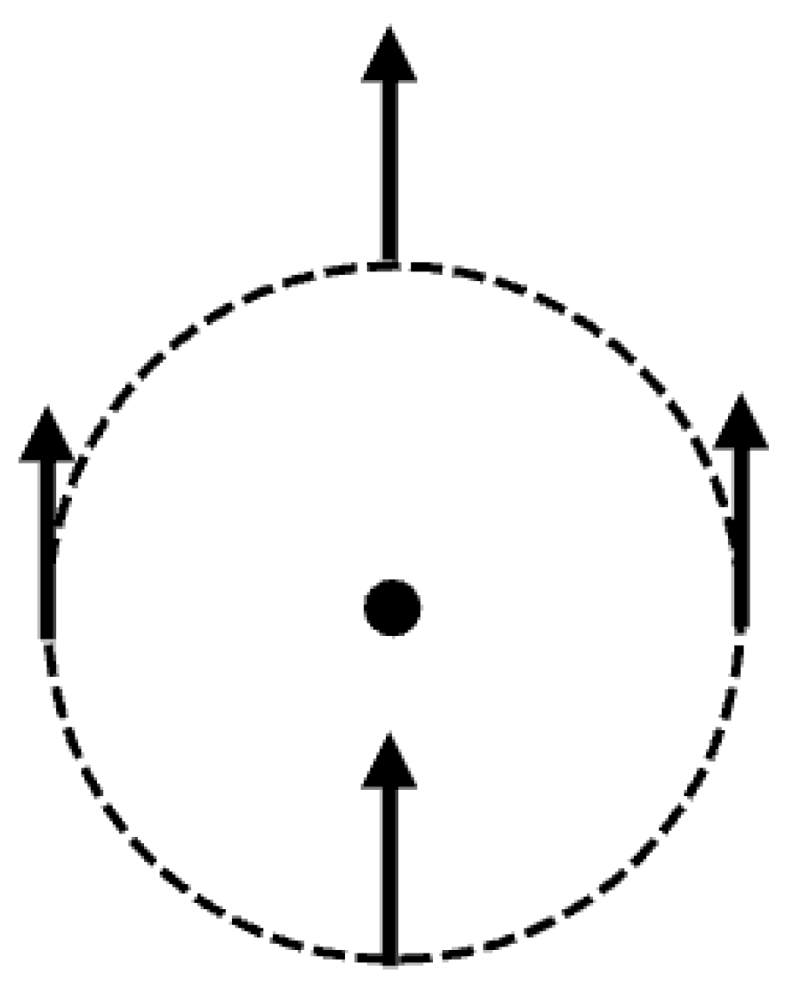
In the figure, we see the gyroscope maintaining its global direction (because we are neglecting geodedic precession) such that at the beginning of the orbit, the gyro points toward the Black Hole, and 180 degrees later it points away from the Black Hole and 180 degrees later it once again faces the Black Hole. If the observer in circular orbit is tidally locked to Black Hole, then in the reference frame of the observer, the Black Hole is always in the same place (i.e., the Black Hole/observer system looks unchanging over time) and it appears that the gyroscope is precessing over time relative to both the observer and the Black Hole. So even though in the observer’s frame the Black Hole’s position relative to the observer is unchanged over time (due to the tidally locked frame of the observer), the precession of the gyroscope in the frame encodes the information about the orbit. In other words, the precession rate of the gyroscope in the observer’s frame is equal to the angular velocity in the exterior metric.

Now suppose we move the frame closer and closer to the Black Hole while always maintaining the same angular velocity (i.e. as the frame moves closer to the Black Hole, the precession rate of the gyroscope does not change). Next imagine that we can shrink the horizon of the Black Hole in space as the observer moves closer until it shrinks to a point in space when the observer reaches it (again, this is just a thought experiment, not an examination of what is/is not possible in terms of event horizons). Since we are keeping the precession constant in this experiment, when the observer reaches this center the precession does not represent the orbital angular velocity of the frame (because the observer is now at the center of the original orbit) but rather it represents the intrinsic spin of the reference frame. This intrinsic spin is what the angular term of the interior metric is measuring.

We don’t even need to shrink the horizon to a point as we did above. If we simply move the observer inside the horizon and have the observer look at a fixed point on the surrounding shell (such that the shell looks static in the observer’s frame, equivalent to the tidal-locked orbit in the exterior metric), then when the observer is inside the horizon, it is no longer revolving around the Black Hole, but the gyroscope will precess relative to the fixed point on the surrounding horizon. This is a consequence of the signature flip of the metric as we go from the exterior metric to the interior metric. In other words, as we cross the horizon in this experiment, the orbital angular velocity of the observer in the exterior metric becomes a spin velocity in the interior metric. All points in the space of the interior metric are at the spatial center of the metric and so it is as though the entire interior metric is the spatial center of the exterior metric (this is why we can always keep our frame at $t=0$ and hyperbolically rotate the space to move around. It is because every point in the interior metric is the spatial center of the shell and so anywhere we are can be labelled $t=0$).

Another way we can look at this situation is as follows: the observer in the interior metric points a gyroscope in some direction and the observer remains fixed relative to the gyroscope. The angular velocity in this situation will manifest itself to the observer as the surrounding shell spinning around the reference frame. If we did the same thing in the exterior metric where the observer is fixed to the gyroscope instead of the Black Hole, then the angular velocity will be manifest as the revolution of the Black Hole around the reference frame.

To summarize, the above arguments show that the angular term of the metric in the interior metric is measuring the spin of the reference frame relative to the surrounding horizon.

IV. Comparing the Interior Schwarzschild and FRW Metrics

We have shown that the interior Schwarzschild metric is a spherically symmetric, homogeneous, and isotropic metric. The same is true of the FRW metric. Furthermore, both metrics have a time dependant scaling of space. So the question is: why is the spacelike portion the FRW metric described with Euclidean spherical coordinates (scaled over time), whereas the interior Schwarzschild metric describes space using a single hyperbolic coordinate t. In both cases, the metric only depends on time so ${\partial }_t$ in the interior metric and ${\partial }_r$ in the FRW metric are Killing vectors.

The difference between these metrics is that the internal Schwarzschild metric is surrounded by an event horizon located infinitely far from all points in space, but a finite distance away in time. Thus time has a spherical character in the Schwarzschild metric.

Comparing the exterior and interior Schwarzschild metrics, we see in the exterior metric that the $dr$ and $rd\Omega$ terms have the same sign. Both of those terms are spacelike intervals in this metric. In the interior metric, the $dr$ and $rd\Omega$ terms are both intervals of time since r has units of time. Yet, these terms have opposite signs in the metric. We can give them the same sign by making the $d\Omega$ term imaginary so that $-{\left(rd\Omega \right)}^2=+{\left(ird\Omega \right)}^2$.

So if we make the azimuthal interval imaginary, this means that $ird\Omega$ is an imaginary time, thus, the interval is spacelike (because if we multiply the differentials of say, the Minkowski metric, by i, then $d{x}^2$ becomes timelike and $d{t}^2$ becomes spacelike). Consider a circle with some radius r. If r has units of time, an arc length drawn on the circle will also have units of time. But since every point on the arc is at the same radius, every event on the arc is at the same time. Therefore, the interval of the arc is spacelike, which is why it is negative in the metric.

Thus we see that the azimuthal term describes a kind of imaginary sphere with a real radius. As has been shown, the arc lengths in the interior metric describe rotations of the reference frame relative to the surrounding shell. This can be thought of as the ’spin’ of the reference frame and the spin space described by the azimuthal term is an imaginary 2-sphere.

V. Conclusion

It has been demonstrated that the Kantowski-Sachs-like interior metric of the Schwarzschild solution is homogeneous and isotropic. The azimuthal scale factor, which has up to now led to the belief that the interior metric was anisotropic is shown to measure the change in orientation of reference frames relative to the surrounding horizon known as Thomas precession. The acceleration of the Thomas precession results in the inertial acceleration of the tangential and angular velocities of frames travelling on circular paths. The analysis was only applied to circular paths, but does apply to arbitrary curved paths. It was shown that the azimuthal term of the exterior metric characterizes the orbital velocity of a reference frame while the azimuthal term of the interior metric characterizes the (classical) spin velocity of a reference frame.

The fact that the interior metric is an isotropic, homogeneous vacuum has implications for cosmology, in particular regarding Dark Energy and Dark Matter effects. These cosmological implications will be the subject of a follow-up work.

References

- Doran, R. Interior of a Schwarzschild Black Hole Revisited. Found Phys 2008, 38, 160–187. [Google Scholar] [CrossRef]
- Figure 1 is a modification of: ’Kruskal diagram of Schwarzschild chart’ by Dr Greg. Licensed under CC BY-SA 3.0 via Wikimedia Commons. http://commons.wikimedia.org/wiki/File:Kruskal_diagram_of_Schwarzschild_chart.svg#/media.
- Hestenes, D. New Foundations for Classical Mechanics; Springer Dordrecht, 1999.
- Carroll, S.M. Lecture Notes on General Relativity, 1997, [arXiv:gr-qc/9712019v1].
Figure 1.
Common Gravitational Well Depiction of the Schwarzschild Metric
Disclaimer/Publisher’s Note: The statements, opinions and data contained in all publications are solely those of the individual author(s) and contributor(s) and not of MDPI and/or the editor(s). MDPI and/or the editor(s) disclaim responsibility for any injury to people or property resulting from any ideas, methods, instructions or products referred to in the content. |
© 2024 by the authors. Licensee MDPI, Basel, Switzerland. This article is an open access article distributed under the terms and conditions of the Creative Commons Attribution (CC BY) license (http://creativecommons.org/licenses/by/4.0/).
Copyright: This open access article is published under a Creative Commons CC BY 4.0 license, which permit the free download, distribution, and reuse, provided that the author and preprint are cited in any reuse.