
Submitted:
02 October 2025
Posted:
03 October 2025
You are already at the latest version
Abstract
There is a wide spread of rice blast in Africa, Asia and Latin America, leading to significant yield losses. In addition, the vagaries of climate change makes it necessary to develop a resistant variety capable of adapting to varied environmental conditions. This experiment was conducted to select superior genotypes across environments from the advanced blast resistant rice lines. Eighteen improved blast-resistant rice genotypes that were produced by crossing MR219 (susceptible) and Pongsu Seribu-2 (resistant) were assessed in four distinct environments in Malaysia (UPM Serdang; Tanjung Karang, Selangor; Kota Sarang Semut, Kedah and Tanjung Karang, Selangor). MR219 variety was included as a check variety for yield making a total of 19 genotypes evaluated. Three replications in each environment were used in the randomised complete block design experiment. Data on vegetative, yield, and yield component attributes were recorded. For most of the variables under investigation, analysis of variance showed significant differences between genotypes, environment, and GxE interaction. With the exception of the number of panicles and tillers per hill, low genetic advance was also found for every trait. Positive correlation was found between yield per hectare and other agronomic traits evaluated except days to flowering and maturity, plant height, and number of unfilled grains. Three groups of rice genotypes were identified by stability analyses utilizing both univariate (bi, S2d, σi2, Wi2, YSi) and multivariate stability statistics. The first group comprised genotypes with high mean yield traits and good stability, including G18, MR219, G17, and G11. These genotypes had broad environmental adaptations. The second group's genotypes, including G1, G6, and G8, were characterised by low stability but high mean yield traits, making them appropriate for cultivation in a specified environment. The third group comprised genotypes such as G7, G9, and G13 that had high stability but a low mean yield characteristic. Environmental discriminate analyses using GGE biplot revealed that Tanjung Karang 1 was the most appropriate environment for most of the genotypes. Blast disease reaction after challenging with inoculum indicates that 11 genotypes proved resistant to the disease while blast disease screening under protected glass house at Mardi and UPM indicated resistance in 13 and 12 genotypes, respectively. Superior genotypes, specifically G18, G17, G11, G14, and G5, were selected from this study because of their stability and high yielding characteristics across mega environments. Breeders could utilize these genotypes for future improvement programmes.
Keywords:
univariate and multivariate statistics
; GxE
; Magnaporthe grisea
; climate resilience
; adaptation
; Oryza spp.
Introduction
Oryza sativa L. commonly known as rice is grouped in the genus Oryza in the family of grasses, Gramineae (Poaceae). There are 22 species in genus Oryza where 20 are wild species and the other two are cultivated species which are Oryza sativa and Oryza glaberrima [3,4]. The cultivated rice is a significant cereal for human nutrition which is grown in various places and under diverse climatic conditions either through transplanting or direct seeding practices in rainfed or irrigated ecosystems [5,6]. Rice is considered as basic food eaten by a large world population with over 90% production from Asia countries [7,8]. It is one of the major staple grains supplying more than 20% daily calorie intake for more than 3.5 billion people [7,9]. In each 100 g, serving of cooked, unenriched, white, and long-grained rice, contains 130 calories, 68% water, 28% carbohydrates, 3% protein and negligible fat [2,10]. It can be cultivated in various types of soils covering saline, alkaline, and acid-sulfur soils as it functions as the basis to distinguish the type of cultivar, adaptation to tropical or temperate climates and dependency on water during their life cycle [1,2]. Majority of rice cultivation and consumption occur in the Asia. The imposed National Agriculture Policy (DPN3), 1998-2010 and National Agro-Food Policy of Malaysia, 2011-2020 had emphasized that an increase in local rice output is needed to safeguard the country’s demand in future. The production of rice in Malaysia showed an increase in the year 2015 from 1,756 tonnes to 2,252 tonnes in 2016 [2,3]. Recently, due to extreme heat and drought, the Self-Sufficiency Level (SSL) for rice production in Malaysia decreased to 50% affecting about 130,000 acres (52,609.13ha) of paddy fields [5]. The government needs to ensure that the rice supply is adequate for current and future consumption, by encouraging local production of rice and reduce its dependency on imported rice. This would give positive influence on Malaysia’s rice industry and value of Ringgit against other currencies could appreciate.
The Malaysian Agricultural Research and Development Institute (MARDI) developed the commercial Malaysian indica rice variety known as MR219, which was formally released in January 2001. This variety was developed from the cross between MR137 and MR151 [11]. It is a high yielding variety with over 10 t/ha based on a direct seeding planting system at the time of release. This commercial white variety is widely cultivated among farmers for more than 12 years covering more than 90% of Malaysian rice granary field and has significantly increased in production and food security demands [12,13]. According to Alias [11], the characteristics of MR219 are 28-30 mg of single grain weight, up to 200 grains/panicle, low amylose content, short maturation period of 105-111 days, and resistant to brown planthopper and bacterial leaf blight. This variety excels in qualities (in terms of shape and taste) and high in yield, but it is sensitive to a change in environment [14,15]. In recent time, the performances of MR219 had declined because of weed prevalence, pests and diseases especially blast infestations in the rice granary areas. This variety needs a high input of fertilizer and good water management practices before it can produce high yield [16,17]. Pongsu Seribu 2 is a known Malaysian rice variety that holds broad-spectrum resistance towards rice blast disease [18,19]. Studies on blast classification conducted by Malaysian Agricultural Research and Development Institute (MARDI) showed that Pongsu Seribu 2 was the most resistant variety towards all 22 Magnaporthe oryzae pathotypes screened. It was revealed that this variety is resistant towards numerous Malaysian blast pathotypes similar to the parental resistant varieties, such as Tetep from Vietnam and Tadukan from Philippines [20,21]. Fatah et al. [22] and Ashkani et al. [23] reported that blast resistance genes was isolated from Pongsu Seribu 2 and subsequently utilized for development of blast-resistant rice variety suitable for Malaysian climate. Some of the deficiency traits in this landrace include longer days to maturity at 140-148 days, plant height of 128.5 cm, 10-15 tillers and high amylose content.
In univariate stability analysis, the commonly used methods are regression and variance estimates. Stability based on regression model is demonstrated by mean of the trait (M), regression slope (bi) and the sum of squares for deviation from regression (S2d). The stability for variance estimate includes Wrickle’s stability ecovalence (Wi2), Shukla’s stability variance (σi2), and Kang’s yield stability (YSi) [24]. Commonly used multivariate stability analyses are additive main effects and multiplicative interaction (AMMI) model, and genotype main effects plus G×E (GGE) model [24]. The detailed description and difference between AMMI and GGE Biplot model were presented by Yan et al. [25]. These two stability analysis approaches only gave individual stability aspects. The overall genotype’s response picture can be unified using cluster analysis [26]. This method grouped the genotypes based on their response structure that represent a move from ranking stability by a quantitative measure to assorting genotypes into qualitatively homogeneous stability subsets. The advantage of classification is that genotypes were grouped according to a specific data set, the relative relationships among genotypes can be independent of any particular set of data analyzed [27,28]. As the first recorded disease of rice, rice blast is widespread over Asia, Latin America, and Africa causing yield losses amounting to hundreds of millions of tons annually [29,30]. Developing a resistant variety that could adapt to varied environmental conditions owing to the vagaries of climate change could be regarded as a worthwhile effort. Therefore, the objective of this research was to select superior genotypes with high mean yield and stable across environments among the improved genotypes prior to commercial cultivation.
Results
Screening for Blast Disease
The result in Table 1 shows the blast disease reactions of the improved lines. The recurrent parent MR219 was susceptible to M. oryzae pathotype 7.2, whereas the donor parent Pongsu Seribu 1 demonstrated resistance to the disease. Similar result was obtained when the improved lines were challenged by artificial inoculation of the disease and field screening carried out at UPM Rice Research Centre and the Malaysian Agricultural Research Development Institute (MARDI). The results also showed that the improved lines varied in their disease reaction to M. oryzae P7.2. (Table 1).
Stability Analysis
Univariate Stability Measures
Type 1: Regression Slope (bi) and Deviation from Regression (S2d)
The result shows that regression slope value for days to maturity ranged from -0.88 to 1.91 where G5 was chosen as the most stable for this trait followed by G8 and G17. The rank orders for three least stable genotypes were G7 < G12 < G13 (Table 2). In case of plant height, the value observed was between -0.65 and 2.92 and the most stable genotype for this trait was G5 followed by G2 and G6. The last three less stable genotypes were observed by G7, G11 and G12 (Table 2). Values ranging from -1.07 to 2.72 was observed for number of filled grains and G10 was observed as the most stable genotype followed by G6 and G17. G2, G12, and G4 were observed having low level of stability for this trait (Table 3). Similarly, a range from -1.61 to 2.53 was recorded for total grains weight, and MR219 was ranked the best since the significant value bi closer to unity followed by G5 and G2 (Table 3). According to yield per hectare, the values ranged between -1.61 and 2.52 while the best genotype was MR219 followed by G5 and G2. Both traits (total grains weight and yield) considered G10 to be the least stable in ranking followed by G4 and G11 (Table 3). Genotypes that showed higher specificity in adaptation to environments for days to maturity, plant height and number of filled grains were G15, MR219 and G10; G7, G9 and G10; G11, G14 and G9, respectively indicating that such genotypes have bi values greater than unity (bi> 1). For total grains weight and yield traits, the result showed that G10, G4 and G11 had higher sensitivity to changes in the environment. The result showed that G2, G5, G7, G8 and G18 had a significant value of regression deviation for days to maturity. A significant deviation from regression value for plant height was observed by G8 and G13. Similar result was also recorded by G7, G10, G12, G14, G16 and MR219 for number of filled grains. Meanwhile, four genotypes had a significant value of S2d, namely, G1, G2, G6 and G15 for total grains weight and yield per hectare. The mean square values for combined analysis of variance (ANOVA) for traits assessed over four environments are presented in Table 4. The result obtained showed a significant genotype x environment interaction for all the traits assessed across various environments.
Type 2: Shukla stability variance (σi2) and Wrickle’s ecovalence (Wi2)
The result shows that based on days to maturity, the genotypes were ranked as follows; G9> G4> G14> G13> G16 > G5> G1> G3 > G6> G12> G10> G17 > G2> G11 > G15 > G7 > G8> MR219 > G18 (Table 2). For plant height, the genotypes were ranked in the following order; G14> G8> G3> G13> G5> G16> G18> G9> G12> G7> G6> G10 > G15> G4 > G2 > G11 > G1 > G17 > MR219 (Table 2). Also, using number of filled grains, the genotypes were ranked; G7> G17> G9> G4> G5> G16> G6> G8 > MR219> G11> G12> G14 > G18> G13 > G2 > G1 > G3 > G10 > G15 (Table 3). The genotypes stability were ranked using total grains weight (Table 2) and yield (Table 3) as follows; G4 > G13 > G18 > G5 > G7 > G9 > G17 > G14 > G2 > G15> G11> G3> G8 > MR219 > G12> G16> G16 > G10 > G1.
Type 3: Kang stability statistics (YSi)
Days to maturity revealed that besides the commercial rice variety, MR219, other stable genotypes were G3, G4, G5, G9, G11, G12, G16, and G17 (Table 2). Stable genotypes based on plant height were observed by G2, G3, G4, G5, G6, G7, G8, G11, G13, G17, G18, and MR219 (Table 2). According to number of filled grains, the genotypes that were stable are G4, G5, G6, G10, G11, G12, G17, G18, and MR219 (Table 3). Lastly, G5, G8, G11, G14, G17, G18, and MR219 were the genotypes that had stable total grains weight and yield (Table 3).
Spearman Rank Correlation for Univariate Stability Measures
Computation for ranking of genotypes against their univariate stability measures was done using Spearman rank correlations (Table 5). This study showed trait mean (M) was positively and highly significantly correlated only with Kang stability (YSi). Meanwhile, Shukla’s stability (σi2) was positively and highly significantly different against the Wrickle’s ecovalence (Wi2) and Deviation from regression (S2d). Same results also were showed by Wrickle’s ecovalence (Wi2) against Deviation from regression (S2d), and Deviation from regression (S2d) as against Kang’s stability (YSi). A negative and non-significant correlation of regression coefficients (bi) with all other stability measures were recorded for days to maturity. In addition, plant height also was observed with regression coefficients (bi) that was not significant and negatively correlated with trait mean (M), Kang stability (YSi) and Deviation from regression (S2d). Number of filled grains recorded trait mean (M) that had negative and non-significant relationship with other stability measures except Kang’s stability (YSi), and this Kang’s stability (YSi) was recorded with the same result with other measures. Lastly, total grains weight and yield were observed with the negative and non-significant correlation between trait mean (M) with Shukla’s stability (σi2) and Wrickle’s ecovalence (Wi2). Regression coefficients (bi) was negative and no significant correlation was observed in all other variables except Kang’s stability (YSi) and trait mean (M).
Multivariate Stability Analyses
Mega-Environment Analysis: Which-Won-Where Pattern
The result in Figure 1 shows the polygon views of GGE Biplot for which-won-where pattern. Axis 1 represents the principal component 1 (PC1) value that indicates the mean performance, while axis 2 indicates the principal component 2 (PC2) value that represents the level of stability. Bigger value for PC1 value means higher mean and small PC2 value means high stability. The perpendicular line that passes through the biplot origin to the polygon splits the biplot into sectors; each with their own winning genotype. The polygon view of GGE biplot explained the genotype and G×E variation of 76.07, 75.77, 89.62, 77.63 and 77.58% for days to maturity, plant height, number of filled grains, total grains weight and yield per hectare, respectively. For all three traits, one sector consisted of EN2 (Tanjung Karang 2) where G17 won at this environment. Another sector consisted of EN1 (Tanjung Karang 1), EN3 (Kota Sarang Semut) and EN4 (Serdang) where the winning genotype was G11 for plant height, and G17 for total grains weight and yield. As for days to maturity and the number of filled grains, there were three sectors that had environmental markers. Days to maturity revealed one sector had EN4 (Serdang) with G18 as the winning genotype. The second sector consisted of EN2 (Tanjung Karang 2) where G12 won at this environment. The last sector consisted of EN1 (Tanjung Karang 1) and EN3 (Kota Sarang Semut) where G19 (MR219) performed the best at these two environments. For number of filled grains, G3 as the winning genotype won at the first sector that had EN1 (Tanjung Karang 1). EN2 (Tanjung Karang 2) falls into the second sector and G10 won at this environment. Third sector consisted of EN3 (Kota Sarang Semut) and EN4 (Serdang). These environments showed that G6 performs the best. The genotype that performed the best in those environments was indicated by the vertex of a polygon in each sector.
Genotype evaluation: Mean vs Stability
For days to maturity, G12 had the highest mean followed by G3, G9, G11, and G5. The lowest mean was observed by G7, G10 and G8 (Figure 2a). As for number of filled grains, G6 was observed having the highest mean followed by G2, G18 and G19 (MR219) while G15, G10 and G14 had the lowest mean of filled grains (Figure 2c). A high amount of filled grains will directly translate into high yield. Hence, the ideal genotypes based on this trait are the genotypes with high mean and high level of stability as observed by G6, G2, and G18. Total grains weight (Figure 2d) and yield per hectare (Figure 2e) traits were observed. G18 had the highest mean followed by G17, G11, G14, and G5. The G16 was observed with the lowest mean for both traits. According to these two traits, genotypes with high mean and stability is preferred, therefore, G18, G17, and G11 were chosen as ideal genotypes.
Genotype Evaluation: Ranking Genotypes
The biplots showed the concentric circles that indicate the order of genotypes. The genotype positioned inside the inner circle and at the head of the arrow at the centre is considered as ideal genotype. The selection order of an ideal genotype is followed by genotype markers that fall next to the inner circle. In this study, days to maturity showed three genotypes fall inside the inner circle which was G3, G5, and G9 (Figure 3a). These genotypes were considered as ideal genotypes and thus favoured compared to other genotypes. For plant height, there was no genotype that falls inside the circle (Figure 3b). Number of filled grains was observed with no genotype inside the inner circle. Hence, genotype that falls in the next circle is preferred. This trait in most preferred order were observed as follow: G2 > G6 > G19 > G4 > G13> G18 > G17 > G7 > G5 > G3 > G8 > G9 > G11 > G12 > G1 > G16 > G14 > G10 > G15 (Figure 3c). Both biplots for total weight of grains (Figure 3d) and yield per hectare (Figure 3e) showed one genotype falls inside this inner circle which was G18. This means that G18 is the best genotype among the 19 evaluated genotypes based on total weight of grains and yield. It is followed by G19, G17, G11, G5, and G14.
Environmental Evaluation: Discriminative vs Representative
Evaluation of the environments using GGE biplot was done to discover the ability in discriminative and representativeness of tested environments. This study explained 76.07, 75.77, 89.62, 77.63 and 77.58% for days to maturity, plant height, number of filled grains, total grains weight and yield per hectare, respectively, for genotypic and genotype by environment variation according to the discriminative and representative view of GGE biplot (Figure 4a). The biplot indicates that the longer the vector, the higher the discriminative power. Meanwhile, the smaller the angle, the higher the representative power. From the graphical displays of test environments evaluation, it can be concluded into three main classifications. First, the environmental markers with a very short vector that is closer to the origin of biplot signifies that the performance of the genotypes was the same in this particular environment. So, little or no details were provided about discrimination or differences of genotypes. Based on three biplots which are on plant height (Figure 4b), total grains weight (Figure 4d) and yield per hectare (Figure 4e), there was no environmental markers with short vector. However, a short vector of the environmental marker was observed at EN1 (Tanjung Karang 1) and EN4 (Serdang) for days to maturity (Figure 4a), EN2 (Tanjung Karang 2) and EN4 (Serdang) for number of filled grains (Figure 4c).
Next is the environment marker that has long vector with big angle originating from AEC line. Selection of superior genotype cannot be made based on this environmental marker, but it can help in choosing unstable genotypes. EN2 (Tanjung Karang 2) and EN3 (Kota Sarang Semut) for days to maturity (Figure 4a) while EN1 (Tanjung Karang 1) for number of filled grain (Figure 4c) markers were observed with this classification. As for other three traits, EN2 (Tanjung Karang 2), EN3 (Kota Sarang Semut) and EN4 (Serdang) markers were observed with long vector and big angle. These revealed that these environments can be utilized to assist in discriminating genotypes with unstable performance based on each trait. Hence, the genotypes with poor performance can be cut out and thus reducing the list of improved genotypes to be selected as a superior genotype. Lastly, classification based on where environmental markers have long vector but small angle nearer to the AEC line implies that this environment can be a representative of a mega-environment. No environmental markers with these characters were observed for days to maturity. Number of filled grains was observed with this marker for EN3 (Kota Sarang Semut). Other three traits, were observed with EN1 (Tanjung Karang 1) marker had long vector and small angle. Evaluation in these environments will greatly help in identification of the ideal genotype among the improved lines.
Environmental Evaluation: Ranking of Environments
The biplots showed the environments ranking view of GGE biplot that accounted 76.07, 75.77, 89.62, 77.63 and 77.58% for days to maturity, plant height, number of filled grains, total grains weight and yield per hectare, respectively, for genotypic and genotype by environment variation (Figure 5). The best environment is indicated by an environmental marker located at the centre in the inner concentric circle. The selection of environment is followed by markers that positioned in the next circle. These environments can be referred to as the favourable environment. The poorest environment in discriminating the genotypes is indicated by marker that located outside the circle. All five traits were not observed with environmental markers that fall in inner circle. The order of environments selection for days to maturity (Figure 5a) was EN2 (Tanjung Karang 2) > EN3 (Kota Sarang Semut) > EN1 (Tanjung Karang 1) > EN4 (Serdang). Plant height (Figure 5b) was EN1 (Tanjung Karang 1) > EN4 (Serdang)> EN3 (Kota Sarang Semut) > EN2 (Tanjung Karang 2). Number of filled grains (Figure 5c) was EN1 (Tanjung Karang 1) > EN3 (Kota Sarang Semut) > EN4 (Serdang) > EN2 (Tanjung Karang 2) and for both total grains (Figure 5d) and yield per hectare (Figure 5e) traits were EN1 (Tanjung Karang 1) > EN4 (Serdang) > EN3 (Kota Sarang Semut) > EN2 (Tanjung Karang 2). For total grains weight and yield per hectare, EN2 (Tanjung Karang 2) was considered the poorest environment since its marker located outside the circle.
Additive Main Effects and Multiplicative Interaction 1 (AMMI1)
Biplot for AMMI1 showed the abscissa that represents the first principal component (PC1) term and ordinate that represents trait main effect. Rice genotypes were well adapted in general environments (stable) when the scores of PC1 is closer to zero. This indicates there are small interaction effects while genotypes were specifically adapted to an environment if PC1 value is larger. Same sign on the PCA axis by the genotypes and environments represents a positive interaction while different sign represents a negative interaction. EN1 (Tanjung Karang 1) had PCA1 score nearest to zero in four traits (Figure 6) evaluated, except plant height (Figure 6b) where EN3 (Kota Sarang Semut) and EN4 (Serdang) were observed nearest to zero value of PCA1. This indicated a small interaction effect for each trait that was present at these environments and signify that the genotypes performed well in this environment. So, Tanjung Karang 1 is considered as the best environment for genotypes evaluation. General adaptation to the environment can be seen for days to maturity by G14, G13, G19, G16 and G15 (Figure 6a), plant height by G8, G15, G17, G19 and G9 (Figure 6b), and number of filled grains by G15, G18, G6, G13 and G5 (Figure 6c). This is because these genotypes had PCA1 value near to zero that signify small interaction and fewer environment influences. However, for number of filled grains, G6, G13, and G5 had low mean of filled grains. Thus, these genotypes can be changed to G10 and G4 that had greater amount of filled grains since this trait positively influenced the final yield. Meanwhile, genotypes such as G3, G7, G5, G19 and G14 had the score of PCA1 that was almost close to zero for total grains weight (Figure 6d) and yield per hectare (Figure 6e). This signifies less influences by the environment on these genotypes. Since the final yield is the ultimate aim by plant breeders, these genotypes except G3 cannot be selected due to having low mean traits. Thus, G15, G11, and G18 that had high yield can be selected for further improvement since it also has the score that was near to zero which indicates general adaptation to the environment.
Discussion
The pooled analysis of variance (ANOVA) for combined environments showed significant differences (p<0.05) among genotypes for all traits except for days to maturity, number of filled grains and number of total grains. Similarly, G×E interaction also recorded significant differences (p<0.05) for assessed traits except for number of tillers and the number of panicles per hill. This result corresponds with Ullar et al. [31] who reported highly significant differences in agronomic traits of in wheat genotypes assessed for genotype x environment interaction and heritability for selection. Oladosu et al. [32] also reported similar result in yield and yield related traits of established and mutant rice genotypes assessed for genotype x environment interaction and stability analyses in Malaysia’s varied environments. Highly significant differences (P≤0.01) were observed among the environments. These reveal the existence of genetic variation at a considerable amount among the evaluated genotypes. The results of Yadav et al. [33] depicted genotype x environment interaction, revealing subtle variations in response to environmental conditions. Means comparison using Tukey test showed differences in performances of each genotype and environment by each trait. All the 13 traits recorded low value of heritability. This is the same for genetic advance where all traits recorded low value, except for number of tillers and number of panicles that recorded moderate value. Ogunniyan and Olakojo [34] reported comparatively lower heritability for grain yield of maize and low genetic advance expected for days to anthesis, days to silking and number of leaves per plant. Correlation coefficients showed that yield per hectare was highly significant and positively correlated with nine evaluated traits but negative correlation with total number of grains. This result implies that increase in most of the agronomic traits studied would result to selection for high yield [28,35,36]. Days to flowering, days to maturity and plant height observed a non-significant correlation with the yield per hectare.
The result obtained from this work shows that 11 genotypes proved resistant when challenged with blast pathogen while blast disease screening under protected glass house at Mardi and UPM indicated resistance in 13 and 12 genotypes, respectively. Crop genetic improvement aims to develop new, improved crop varieties that have higher yield, better quality of grain, improved disease (bacterial, fungal, or virus) and insect pest resistance [9,18]. Over the ages, classical breeding methods had been used for incorporation of major R genes to develop new rice variety, but now it is more convenient to use marker-assisted selection (MAS) to accelerate and precisely introduce the major and minor R genes [18,21]. Many efforts have been made towards the development of durable resistant blast rice varieties [9]. Molecular markers have been widely applied to identify and map genes regarding complete and partial resistance [9,18,23]. The incorporation of resistance (R) genes into rice is the best way to combat with rice blast disease since it is effective, economical, and environmentally safe [9]. Resistance is a viable method of controlling rice blast disease. Achieving a stable resistance to blast is the best way to manage blast disease due to the diversity in M. oryzae isolates and variance in pathogenicity of disease [18,23]. Details on the diversity of pathogen are important for sufficient utilization of resistant varieties, and to develop strategies for enhancing the durability of resistance. Selection of right plant with noted characteristics will help in the selection of a superior plant with blast resistance gene of interest.
Crop breeders need detailed information on nature and magnitude of genotype by environment interaction (G×E) for any new variety approaching commercial release. Data on multi-environmental trials are commonly analyzed using analysis of variance (ANOVA), but it has restriction in ability to discriminate the significant difference of genotype in a non-additive term called G×E [37]. This caused the development of stability statistical methods to evaluate the stability of genotypes in order to determine the genotype that performed consistently in adverse environments. When a significant interaction for G×E was determined, further stability analysis was performed for better understanding of the tested genotypes performance across environments to identify the level of stability. Univariate stability are categorized into three types which are Type 1, comprised of Regression Slope (bi) and Deviation from Regression (S2d), Type 2, comprised of Shukla stability variance (σi2) and Wrickleecovalence (Wi2), and Type 3, which is Kang stability statistics (YSi) [38,39]. Additionally, adjusted traits mean (M) and least significant differences for G×E were computed for all 13 traits studied. Multivariate stability is used when there are two or more dependent variables to analyze the patterns of interaction [38,40]. A popular graphical technique for identifying the best genotypes that are either highly stable across environments or exclusively appropriate for a certain environment is the use of biplots, which show the pattern of interactions between genotypes, environments, and G×E interactions [27,35].
Results from univariate and multivariate stability analyses can be summarized to mega-environment, genotype and test environment evaluation. Based on parameters used in this analyses (bi, S2d, σi2, Wi2, YSi, GGE and AMMI biplot), these improved genotypes can be classified into three groups. Firstly, the genotypes having high yield along with high stability as seen in G18, MR219, G17, and G11. These genotypes were widely adapted to adverse environments and thus can be selected as the ideal genotype among the evaluated genotypes. Elakhdar et al. [41] noted that the study of genetic variability through phenotypic characterisation is essential in a breeding programme. Hence, assessing both yield attributes and stability across mega environment is crucial to select stable and yield yielding cultivars. Secondly, the genotypes with high mean of yield but low level of stability such as G1, G6 and G8 were fit for a particular environment. Lastly, the genotypes with low mean of yield per hectare but high stability indicated these genotypes were suitable for breeding of specific traits (G13, G9, and G7). In the study involving simultaneous selection of high yielding and most stable genotypes using non-parametric methods, Sabaghnia et al. [42] noted that it is important to explain G x E interaction in breeding programme because effects due to environment is usually greater than genetic effects in multi-environmental trials. Cluster analysis using UPGMA dendrogram grouped 19 genotypes into six major groups based on the assessed traits. The largest group was Group 1 which consisted of eight genotypes, while Group II, IV and VI were the smallest group with one genotype in each group. The commercial variety, MR219 was grouped with G17 and G18 in Group III [26,43].
Value of regression coefficient (bi) for each genotype that is close to unity (bi= 1) (P < 0.01) together with high trait mean is found to be stable over adverse environments [44]. Genotypes are labelled as badly acclimatized to environments when associated with low trait mean performance. Whilst a bi higher than unity(bi> 1) indicates that the genotypes are more sensitive to environmental changes and greater specificity of adaptability to high yielding environments. Deviation from regression (S2d) considered genotypes to be stable when its value is not significantly different from zero [45]. Shukla stability variance (σi2) and Wricke’s ecovalence (Wi2) considered genotypes with low value as stable [46]. Thus, genotype having the lowest stability of variance are classified as the most stable and are at the top in rank. Following this method, the genotype with a value of YSi greater than the overall average of YSi value is considered to be stable.
The GGE biplot graphs help to make comparison among genotypes across environment within mega-environment that was based on the mean performance and stability. This study explained 76.07, 75.77, 89.62, 77.63 and 77.58% for days to maturity, plant height, number of filled grains, total grains weight and yield per hectare, respectively, for genotypic and genotype by environment variation according to the mean vs stability view of GGE biplot. A short maturity date is preferred by breeders since it signifies short life cycle. Thus, the ideal genotypes according to this trait are G7, G10, and G8 that had the lowest mean and also high stability level. The highest mean of plant height was observed on G11 followed by G18, G19 (MR219), G17 and G5. While G16, G7, and G15 were observed with the lowest mean (Figure 2b). Breeders favour short or moderate plant height since it affects the translocation of nutrition and prevent lodging. So, G16, G7 and G15 were the ideal genotypes based on this trait due to having a low mean of height and high stability. According to Yan & Kang [47] and Yan [48], an average environment coordinate (AEC) which is the average of environmental PC1 and PC2 scores were indicated by small circle at the centre of a biplot. The mean of trait was indicated by the single arrowed line of average environment axis (AEA) that passes through the small circle (AEC) via origin of biplot. The genotypes were ranked according to the direction of the arrow on AEC abscissa in increasing order; the arrow pointing towards higher trait mean. Thus, the genotype with highest mean performance will be positioned to the right. Meanwhile, the double-headed arrow perpendicular line to AEA passing through the origin of biplot represents the level of stability. The level of genotypes stability was determined by the projection of AEC vertical axis where the shortest projection from the AEC axis indicated higher stability. Longer projection on the AEC abscissa indicates highly unstable genotypes irrespective of its direction. The ideal genotype is the genotype having high mean performance and level of stability as proposed by Yan &Tinker [49]. The which-won-where pattern reveals which genotype win at which environment. The winning genotype can be seen at the vertex where the two sides of polygon meet whose perpendicular lines forms the boundary of the sector. A single genotype is considered having the best performance in all tested environments when all environmental markers are positioned into one sector. However, different genotype won in different environment when environmental markers were positioned on different sector. Genotype is considered has poor performance if it is located at the vertex where no environmental markers presence [2,47]. The different points of environment and genotype winning in each sector confirmed that there was an influence of G×E interaction on the genotype performances for the evaluated traits. Meanwhile, in the sector where no environmental marker falls showed that these genotypes located in this sector were poorly performed over environments. In addition, those genotypes within the polygon reflect low response to the environment than the genotype at the vertex [32].
Conclusions
Based on the results obtained, significant differences were found among genotypes, environments and G×E interaction for most of the evaluated traits under study. Correlation analysis also showed most traits were significantly and positively related to the yield per hectare. Eleven genotypes proved resistant when challenged with blast disease while screening under protected glass house at Mardi and UPM indicated resistance in 13 and 12 genotypes, respectively. Univariate and multivariate stability parameters revealed that these genotypes were classified into three groups. The ideal environment for the cultivation of improved genotypes is Tanjung Karang 1. The selected genotypes would perform best in this environment. All environments showed high discriminative and representative ability. However, only Tanjung Karang 2 showed less ability of being a representative environment. The selected superior genotypes with high yield and stability among the improved rice lines were G18, G17, G11, G14, and G5. The selected blast-resistant lines were identical to MR261 in terms of high yielding, with potentials as a donor parent for blast-resistance gene. These genotypes could be utilized by breeders for further improvement programmes since yield is controlled by many traits.
Materials and Methods
Planting Materials
Eighteen genotypes of BC2F2 generations were collected from an advance-backcross of MR219 x Pongsu Seribu 2. Introgression lines were developed from these parents through backcross breeding using marker-assisted backcross selection (MABS) strategy producing BC2F2 generation [50]. Pongsu Seribu 2 (PS2) possesses broad-spectrum resistance to blast fungal isolates, which was developed by Malaysian Rice Research Centre, Malaysian Agricultural Research and Development Institute (MARDI) and used as donor parent having blast-resistant gene. With a good grain quality and good eating quality, MR219 possesses a high yield potential. Regretfully, this variety is quite vulnerable to blast. The MR219 and 18 advanced breeding lines were evaluated in a mega-environmental field test. The improved rice genotypes’ stability was tested and their growth performance evaluated in multi-environmental field trials conducted between 2015 and 2017 in four different planting environments (UPM Serdang; Tanjung Karang, Selangor; Kota Sarang Semut, Kedah and Tanjung Karang, Selangor) covering diverse climatic conditions for rice planting area in Peninsular Malaysia. The environments also represent the conditions of major rice granary areas in Malaysia, except Serdang that acts as the reference environment.
Field Experiment
A randomised complete block design (RCBD) with three replications was used to set up the field experiment in each environment. The total size of the plot was 65 m2 of which the length and width are 16.25 m and 4 m. The subplot size for each replication is 4 by 4 m. There was a walking path of 1 m between the replicated plots. The spacing between and within plant was 25 cm. At 21 days, one seedling per hill was transplanted manually to the rice field in each environment. In order to prepare the seedlings for planting, seed dormancy was first broken by oven drying them for 24 hours at 40 degrees Celsius. In order to promote pre-germination, the seeds were completely submerged in water in a petri dish for the whole night. The seeds were kept wet for three days after the water was drained. Water was added to the seeds to keep them moist and prevent drying out. Three days later, the seeds were moved to previously prepared plastic trays packed with soil. Before transplanting to the field, the seedlings were allowed 21 days to grow in the nursery. Every cultural practice, from clearing the ground to harvesting, was carried out in accordance with MARDI’s recommendations. Throughout the studies, the soil was watered with average 10 cm water above sea level. The MARDI prescribed rate for fertiliser, pesticides, and insecticides was followed [51]. For narrow-leafed plants, hand weeding was done on a regular basis to prevent interspecific competition. Broadleaf was treated with contact herbicides designed specifically for broad leaves.
Blast Resistance Screening
Challenging of the Lines
Homozygous seedlings that possess resistance genes were selected and subsequently screened against M. oryzae P7.2. Seedlings that were twenty-one days old were challenged by applying a conidial suspension containing 1.5 × 10⁵ spores per mL along with Tween-20 (0.5 mL per L), following the methodology outlined by Chen et al. [52]. The inoculated seedlings were maintained at a temperature range of 25 to 30 degrees Celsius. To ensure high humidity levels, distilled water was sprayed to the seedlings three times daily. Seven days post-inoculation, the response of each rice line to blast was recorded using a 0–5 disease scoring scale. Responses were classified as follows: scores of 0 to 2 indicate resistance, a score of 3 signifies moderate resistance, and scores ranging from 4 to 5 denote susceptibility to blast [53]. The resistant genotypes underwent additional testing at two different field locations.
Field Screening for Blast Resistance
Each of the promising lines generated above was assessed for its response to blast under a protective blast screening net house at two distinct locations: the UPM Rice Research Center and the Malaysian Agricultural Research Development Institute (MARDI). Each line was planted in a row measuring 50 cm in length within a protected blast screening glass house, maintaining a spacing of 10 cm between rows. A series of plants vulnerable to blast were interspersed after every five plants, as well as along the borders, to guarantee uniform distribution of the disease. Data was collected to show the plants’ responses to the blast, using a scale of 0 to 9, recorded in triplicate at intervals of 10 days, beginning 30 days after sowing. The lines with scores ranging from 0 to 3 were classified as resistant, while those scoring between 4 and 5 were deemed moderately resistant. Scores of 6 indicated moderate susceptibility, and scores from 7 to 9 were categorized as susceptible [53].
Data Collection
Thirteen quantitative traits covering vegetative, yield, and yield components were the subjects of data collection. Five plants from each genotype in each block were sampled following the International Rice Research Institute [54] procedure. However, two traits were observed on plot basis which includes days to flowering and days to maturity. Data collection procedure is as presented in Table 6.
Statistical and Stability Analysis
Univariate Stability Analyses
The recorded data on agro-morphological and yield traits were analysed based on the 19 genotypes’ growth performance and their stability in four environments was tested. In order to determine the different response of evaluated genotypes in each environment as a result of G×E interaction, the data were subjected analyses. Univariate stability analysis was performed using SAS software (version 9.4). The SASG×E (SAS program) is a flexible, capable and efficient program that can analyze many dependent variables simultaneously using multi-environmental trial data. It computed univariate stability statistics, producing input files that are ready to use in existing R packages for multivariate stability statistics, ANOVA, descriptive statistics and the correlation of stability analysis methods. The significance of G×E interaction was tested using ANOVA. However, ANOVA has constraint where it is unable to differentiate the level of genotype in G×E interaction. Thus, additional statistical methods have been developed for further evaluation of genotypes stability, which reflects different aspects of G×E interaction. The SAS G×E code of SAS programme version 9.4 was used to calculate ANOVA for genotype, environment and G×E interaction on all evaluated traits. The output from SAS G×E contains univariate stability result that can be used as an input file for multivariate analysis in R package. Where significant G×E interaction was found, then further statistical analyses (univariate and multivariate) were carried out to identify genotypes’ level of stability and thus determine the ideal genotypes with constant performance across tested environments. For univariate stability, the parameter measured was the slope of regression (bi), deviation from regression (S2d), Shukla’s stability variance (σi2), Wrickle’s ecovalence (Wi2), and Kang’s stability statistic (YSi) with addition mean of traits (M). All pairs of univariate stability measures were calculated for Spearman rank correlation coefficients.
Multivariate Stability Analyses
In this study, cluster analysis and biplots were used to analyze G×E data to see the patterns of interaction. Biplots model that were used is genotype main effects and genotype × environment interaction effects (GGE biplots) and the additive main effects and multiplicative interaction (AMMI biplots). A simplified version of R statistical software, R studio was employed to compute GGE biplots and AMMI. The package used for GGE biplots was GUI package [55], meanwhile, Agricolae package was used for AMMI Model [56]. Both GGE biplots and AMMI were used to visualize the existence of G×E interaction and rank the genotypes based on the mean of traits and level of stability. The produced graphs were based on (i) Mega environment (ii) Genotype evaluation (iii) Tested environment. GGE biplot was constructed graphically using MET data by simultaneously plotting the two (or more) PC scores of genotypes and environments. The PC scores were generated by subjecting the GGE data to singular value decomposition, thus reducing the influence from the environment (E) main effects. There were five types of graph generated using GGE Biplot per trait that explained the change in the ranking of genotypes and also environments due to G×E interaction. Mega-environment analysis helps to point out the specific genotypes that is suitable for a particular mega-environments. Genotype evaluation assesses the genotypes mean performance and its stability in each environment. Whilst environmental evaluation can differentiate the genotypes in target environments. The graphs generated were based on; (i) Which-won-where pattern, (ii) Mean vs stability, (iii) Ranking genotype, (iv) Discriminative and representative and (v) Ranking environment.
Funding
This study was funded by the Malaysian Government through the Higher Institution Centre of Excellence (HiCoE) Research Grant award with the Grant No: 6369105.
Data Availability Statement
The datasets used in this study are available from the corresponding author upon reasonable request @ schukwu@unam.na or mrafii@upm.edu.my.
References
- Oladosu, Y., Rafii, M. Y., Samuel, C., Fatai, A., Magaji, U., Kareem, I., ... & Kolapo, K. (2019). Drought resistance in rice from conventional to molecular breeding: a review. International journal of molecular sciences, 20(14), 3519. [CrossRef]
- Ab. Halim, A. A. B., Rafii, M. Y., Osman, M. B., Oladosu, Y., & Chukwu, S. C. (2021). Ageing effects, generation means, and path coefficient analyses on high kernel elongation in mahsuri mutan and basmati 370 rice populations. BioMed research international, 2021(1), 8350136. [CrossRef]
- Sarif, H. M., Rafii, M. Y., Ramli, A., Oladosu, Y., Musa, H. M., Rahim, H. A., ... & Chukwu, S. C. (2020). Genetic diversity and variability among pigmented rice germplasm using molecular marker and morphological traits. Biotechnology & Biotechnological Equipment, 34(1), 747-762. [CrossRef]
- Brar, D. S., & Khush, G. S. (2003). Utilization of Wild Species of Genus Oryza in Rice Improvement. In: Nanda, J.S., &Sharma, S.D. (Eds.),Monograph of Genus Oryza(pp. 283–309). UK: Science Publishers.
- Oginyi, J. C., Chukwu, S. C., Paul, K. U., & Mkpuma, K. C. (2024). Genetic diversity and stability analysis based on agro-morphological traits among rice genotypes developed through marker-assisted backcrossing. Int J, 10(5), 148. [CrossRef]
- Maclean, J., Hardy, B., & Hettel, G. (2013). Rice Almanac: Source Book for One of the Most Important Economic Activities on Earth. Los Banos, Philippines: IRRI. 283 pp.
- Chukwu, S. C., Rafii, M. Y., Ramlee, S. I., Ismail, S. I., Hasan, M. M., Oladosu, Y. A., ... & Olalekan, K. K. (2019). Bacterial leaf blight resistance in rice: a review of conventional breeding to molecular approach. Molecular biology reports, 46, 1519-1532. [CrossRef]
- Chukwu, S. C., Rafii, M. Y., Ramlee, S. I., Ismail, S. I., Oladosu, Y., Okporie, E., ... & Jalloh, M. (2019). Marker-assisted selection and gene pyramiding for resistance to bacterial leaf blight disease of rice (Oryza sativa L.). Biotechnology & Biotechnological Equipment, 33(1), 440-455. [CrossRef]
- Chukwu, S. C., Rafii, M. Y., Ramlee, S. I., Ismail, S. I., Oladosu, Y., Kolapo, K., ... & Ahmed, M. (2019). Marker-assisted introgression of multiple resistance genes confers broad spectrum resistance against bacterial leaf blight and blast diseases in Putra-1 rice variety. Agronomy, 10(1), 42. [CrossRef]
- USDA. (2017). World Agricultural Production. Foreign Agricultural Service Circular Series WAP 08-17 August 2017.
- Alias, I. (2002). MR 219, A New High-Yielding Rice Variety with Yields of More Than 10 MT/Ha. MARDI, Malaysia. FFTC (Food and Fertilizer Technology Center): An International Information Center for Small Scale Farmers in the Asian and Pacific Region. Retrieved from http://www.fftc.agnet.org/library.php?func=view&id=20110725142748&type_id=8.
- Fasahat, P., Muhammad, K., Abdullah, A., & Ratnam, W. (2012). Proximate Nutritional Composition and Antioxidant Properties of Oryza rufipogon, a Wild Rice Collected from Malaysia Compared to Cultivated Rice, MR219. Australian Journal of CropScience, 6(11), 1502-1507.
- Ibrahim, S. A., Mohd, Y. R., Mohd, R. I., Shairul, I. R., Noraziyah, A. A. S., Asfaliza, R., ... & Momodu, J. (2021). Evaluation of inherited resistance genes of bacterial leaf blight, blast and drought tolerance in improved rice lines. Rice Science, 28(3), 279.
- Panjaitan, S. B., Abdullah, S. N. A., Aziz, M. A., Meon, S., & Omar, O. (2009). Somatic Embryogenesis from Scutellar Embryo of Oryza sativa L. var. MR219. Pertanika Journal of Tropical Agricultural Science, 32(2), 185-194.
- Salleh, S. B., Rafii, M. Y., Ismail, M. R., Ramli, A., Chukwu, S. C., Yusuff, O., & Hasan, N. A. (2022). Genotype-by-environment interaction effects on blast disease severity and genetic diversity of advanced blast-resistant rice lines based on quantitative traits. Frontiers in Agronomy, 4, 990397. [CrossRef]
- Razak, A. H., Suhaimi, O., & Theeba, M. (2012). Effective Fertilizer Management Practices for High Yield Rice Production of Granary Areas in Malaysia. Kuala Lumpur, Malaysia: Strategic Resource Research Centre, Malaysian Agricultural Research and Development Institute (MARDI).
- Oladosu, Y., Rafii, M. Y., Arolu, F., Chukwu, S. C., Muhammad, I., Kareem, I., ... & Arolu, I. W. (2020). Submergence tolerance in rice: Review of mechanism, breeding and, future prospects. Sustainability, 12(4), 1632. [CrossRef]
- Rahim, H. A., Bhuiyan, M. A. R., Saad, A., Azhar, M., & Wickneswari, R. (2013). Identification of Virulent Pathotypes Causing Rice Blast Disease (‘Magnaporthe oryzae’) and Study on Single Nuclear Gene Inheritance of Blast Resistance in F2 Population Derived from Pongsu Seribu 2 x Mahshuri. Australian Journal of Crop Science, 7(11), 1597-1605.
- Akos, I. S., Yusop, M. R., Ismail, M. R., Ramlee, S. I., Shamsudin, N. A. A., Ramli, A. B., ... & Chukwu, S. C. (2019). A review on gene pyramiding of agronomic, biotic and abiotic traits in rice variety development. International Journal of Applied Biology, 3(2), 65-96.
- Rahim, H. (2010). Genetic Studies on Blast Disease (Magnaporthe grisea) Resistance in Malaysian Rice. Dissertation, Universiti KebangsaanMalaysia.
- Chukwu, S. C., Rafii, M. Y., Ramlee, S. I., Ismail, S. I., Oladosu, Y., Muhammad, I. I., ... & Yusuf, B. R. (2020). Recovery of recurrent parent genome in a marker-assisted backcrossing against rice blast and blight infections using functional markers and SSRs. Plants, 9(11), 1411. [CrossRef]
- Fatah, T., Rafii, M. Y., Rahim, H. A., Azhar, M., & Latif, M. A. (2014). Cloning and Analysis of QTL Linked to Blast Disease Resistance in Malaysian Rice Variety Pongsu Seribu 2. International Journal of Agriculture and Biology, 16(2), 395-400.
- Ashkani, S., Rafii, M. Y., Rahim, H. A., & Latif, M. A. (2013). Genetic Dissection of Rice Blast Resistance by QTL Mapping Approach using an F3 Population. Molecular Biology Reports, 40(3), 2503-2515. [CrossRef]
- Dia, M., Wehner, T. C., & Arellano, C. (2017). RGxE: An R Program for Genotype × Environment Interaction Analysis. American Journal of Plant Sciences, 8(07), 1672-1698. [CrossRef]
- Yan, W., Kang, M. S., Ma, B., Woods, S., & Cornelius, P. L. (2007). GGE Biplot vs. AMMI Analysis of Genotype-by-Environment Data. Crop Science, 47(2), 643-653.
- Sabri, R. S., Rafii, M. Y., Ismail, M. R., Yusuff, O., Chukwu, S. C., & Hasan, N. A. (2020). Assessment of agro-morphologic performance, genetic parameters and clustering pattern of newly developed blast resistant rice lines tested in four environments. Agronomy, 10(8), 1098. [CrossRef]
- Ebem, E. C., Afuape, S. O., Chukwu, S. C., & Ubi, B. E. (2021). Genotype× environment interaction and stability analysis for root yield in sweet potato [Ipomoea batatas (L.) Lam]. Frontiers in Agronomy, 3, 665564. [CrossRef]
- Chukwu, S. C., Ekwu, L. G., Onyishi, G. C., Okporie, E. O., & Obi, I. U. (2013). Correlation between agronomic and chemical characteristics of maize (Zea mays L.) genotypes after two years of mass selection. International Journal of Science and Research, 4(8), 1708-1712.
- Oladosu, Y., Rafii, M. Y., Magaji, U., Abdullah, N., Miah, G., Chukwu, S. C., ... & Kareem, I. (2018). Genotypic and phenotypic relationship among yield components in rice under tropical conditions. BioMed research international, 2018(1), 8936767. [CrossRef]
- Chukwu, S. C., Rafii, M. Y., Ramlee, S. I., Ismail, S. I., Oladosu, Y., Muhammad, I. I., ... & Nwokwu, G. (2020). Genetic analysis of microsatellites associated with resistance against bacterial leaf blight and blast diseases of rice (Oryza sativa L.). Biotechnology & Biotechnological Equipment, 34(1), 898-904. [CrossRef]
- Ullah, H., Khan, W. U., Alam, M., Khalil, I. H., Adhikari, K. N., Shahwar, D., ... & Adnan, M. (2016). Assessment of G× E interaction and heritability for simplification of selection in spring wheat genotypes. Canadian Journal of Plant Science, 96(6), 1021-1025. [CrossRef]
- Oladosu, Y., Rafii, M. Y., Abdullah, N., Magaji, U., Miah, G., Hussin, G., & Ramli, A. (2017). Genotype× Environment interaction and stability analyses of yield and yield components of established and mutant rice genotypes tested in multiple locations in Malaysia. Acta Agriculturae Scandinavica, Section B—Soil & Plant Science, 67(7), 590-606. [CrossRef]
- Yadav, A., Rahevar, P., Patil, G., Patel, K., & Kumar, S. (2024). Assessment of G× E interaction and stability parameters for quality, root yield and its associating traits in ashwagandha [Withania somnifera (L.) Dunal] germplasm lines. Industrial Crops and Products, 208, 117792. [CrossRef]
- Ogunniyan, D. J., & Olakojo, S. A. (2014). Genetic variation, heritability, genetic advance and agronomic character association of yellow elite inbred lines of maize (Zea mays L.). Nigerian journal of Genetics, 28(2), 24-28. [CrossRef]
- Musa, I., Rafii, M. Y., Ahmad, K., Ramlee, S. I., Md Hatta, M. A., Magaji, U., ... & Mat Sulaiman, N. N. (2021). Influence of wild relative rootstocks on eggplant growth, yield and fruit physicochemical properties under open field conditions. Agriculture, 11(10), 943. [CrossRef]
- Chukwu, S. C., Okporie, E. O., Onyishi, G. C., & Obi, I. U. (2015). Characterization of maize germplasm collections using cluster analysis. World Journal of Agricultural Sciences, 11(3), 174-182.
- Woldemeskel, T. A., Fenta, B. A., Mekonnen, G. A., Endalamaw, H. Z., & Alemu, A. F. (2021). Multi-environment trials data analysis: An efficient biplot analysis approach.
- Hashim, N., Rafii, M. Y., Oladosu, Y., Ismail, M. R., Ramli, A., Arolu, F., & Chukwu, S. (2021). Integrating multivariate and univariate statistical models to investigate genotype–environment interaction of advanced fragrant rice genotypes under rainfed condition. Sustainability, 13(8), 4555. [CrossRef]
- Onyishi, G. C., Harriman, J. C., Ngwuta, A. A., Okporie, E. O., & Chukwu, S. C. (2013). Efficacy of some cowpea genotypes against major insect pests in southeastern agro-ecology of Nigeria. Middle-East Journal of Scientific Research, 15(1), 114-121.
- Eriksson, L., Byrne, T., Johansson, E., Trygg, J., & Vikström, C. (2013). Multi-and Megavariate Data Analysis: Basic Principles and Applications (Vol. 1). Sweden: Umetrics Academy. 521 pp.
- Elakhdar, A., El-Naggar, A. A., El-Wakeell, S., & Ahmed, A. H. (2025). Integrating univariate and multivariate stability indices for breeding clime-resilient barley cultivars. BMC Plant Biology, 25(1), 76. [CrossRef]
- Sabaghnia, N., Hatami-Maleki, H., & Janmohammadi, M. (2017). Simultaneous selection of most stable and high yielding genotypes in breeding programs by nonparametric methods. Agrofor, 2(2). [CrossRef]
- Chukwu, S. C., Okporie, E. O., Chukwu, G. C., Anyanwu, C. C., Teresia, K. N., Awala, S. K., ... & Olalekan, K. K. (2025). Assessment of agro-morphological performance, genetic parameters and clustering pattern of early maturing high yielding maize (Zea mays L.) genotypes developed through NC II. Discover Plants, 2(1), 109. [CrossRef]
- Kumar, B. D., Purushottam, A. P., Raghavendra, P., Vittal, T., Shubha, K. N., & Madhuri, R. (2020). Genotype environment interaction and stability for yield and its components in advanced breeding lines of red rice (Oryza sativa L.). Bangladesh Journal of Botany, 49(3), 425-435. [CrossRef]
- Zibari, A., & Aziz, P. (2024). Genotype x Environment Interaction and Coefficient Regression in Some Genotypes of Faba Bean (Vicia faba L). Pakistan Journal of Life & Social Sciences, 22(2).
- Chukwu, S. C., Ibeji, C. A., Ogbu, C., Oselebe, H. O., Okporie, E. O., Rafii, M. Y., & Oladosu, Y. (2022). Primordial initiation, yield and yield component traits of two genotypes of oyster mushroom (Pleurotus spp.) as affected by various rates of lime. Scientific Reports, 12(1), 19054. [CrossRef]
- Yan, W., & Kang, M. S. (2002). GGE Biplot Analysis: A Graphical Tool for Breeders, Geneticists, and Agronomists. Boca Raton, Florida: CRC Press. 288 pp.
- Yan, W. (2001). GGEbiplot—A Windows Application for Graphical Analysis of Multienvironment Trial Data and Other Types of Two-Way Data. Agronomy Journal, 93(5), 1111-1118. [CrossRef]
- Yan, W., & Tinker, N. A. (2006). Biplot Analysis of Multi-Environment Trial Data: Principles and Applications. Canadian Journal of Plant Science, 86(3), 623-645. [CrossRef]
- Tanweer, F. A., Rafii, M. Y., Sijam, K., Rahim, H. A., Ahmed, F., Ashkani, S., & Latif, M. A. (2015). Introgression of Blast Resistance Genes (Putative Pi-b and Pi-kh) into Elite Rice Cultivar MR219 through Marker-Assisted Selection. Frontiers in Plant Science, 6, 1002. [CrossRef]
- MARDI. (2008). Manual Teknologi Penanaman Padi Lestari. Institut Penyelidikan dan Kemajuan Pertanian Malaysia.
- Chen, S., Xu, C. G., Lin, X. H., & Zhang, Q. (2001). Improving bacterial blight resistance of ‘6078′, an elite restorer line of hybrid rice, by molecular marker--assisted selection. Plant Breeding, 120(2), 133-137..
- Bhatia, D., Sharma, R., Vikal, Y., Mangat, G. S., Mahajan, R., Sharma, N., ... & Singh, K. (2011). Marker--assisted development of bacterial blight resistant, dwarf, and high yielding versions of two traditional Basmati rice cultivars. Crop science, 51(2), 759-770. [CrossRef]
- IRRI. (2013). Standard Evaluation System for Rice, 5th edition. Manila, Philippines: International Rice Research Institute. 55 pp.
- RStudio. (2014). RStudio: Integrated Development Environment for R (Computer Software v0.98.1074). RStudio.Available at:https://www.rstudio.org/(accessed 30 Jun 2018).
- CRAN. (2014). The Comprehensive R Archive Network. Comprehensive R Archive Network for the R Programming Language. Retrieved fromhttp://cran.r-project.org/web/packages/available_packages_byname.html#available-packages-A(accessed 28 April, 2018).
Figure 1.
GGE Biplot analyses for which won where. Note: A=days to maturity, B=plant height, C=no. filled grains, D=total grains weight per hill, E=Yield per hectare.
Figure 1.
GGE Biplot analyses for which won where. Note: A=days to maturity, B=plant height, C=no. filled grains, D=total grains weight per hill, E=Yield per hectare.
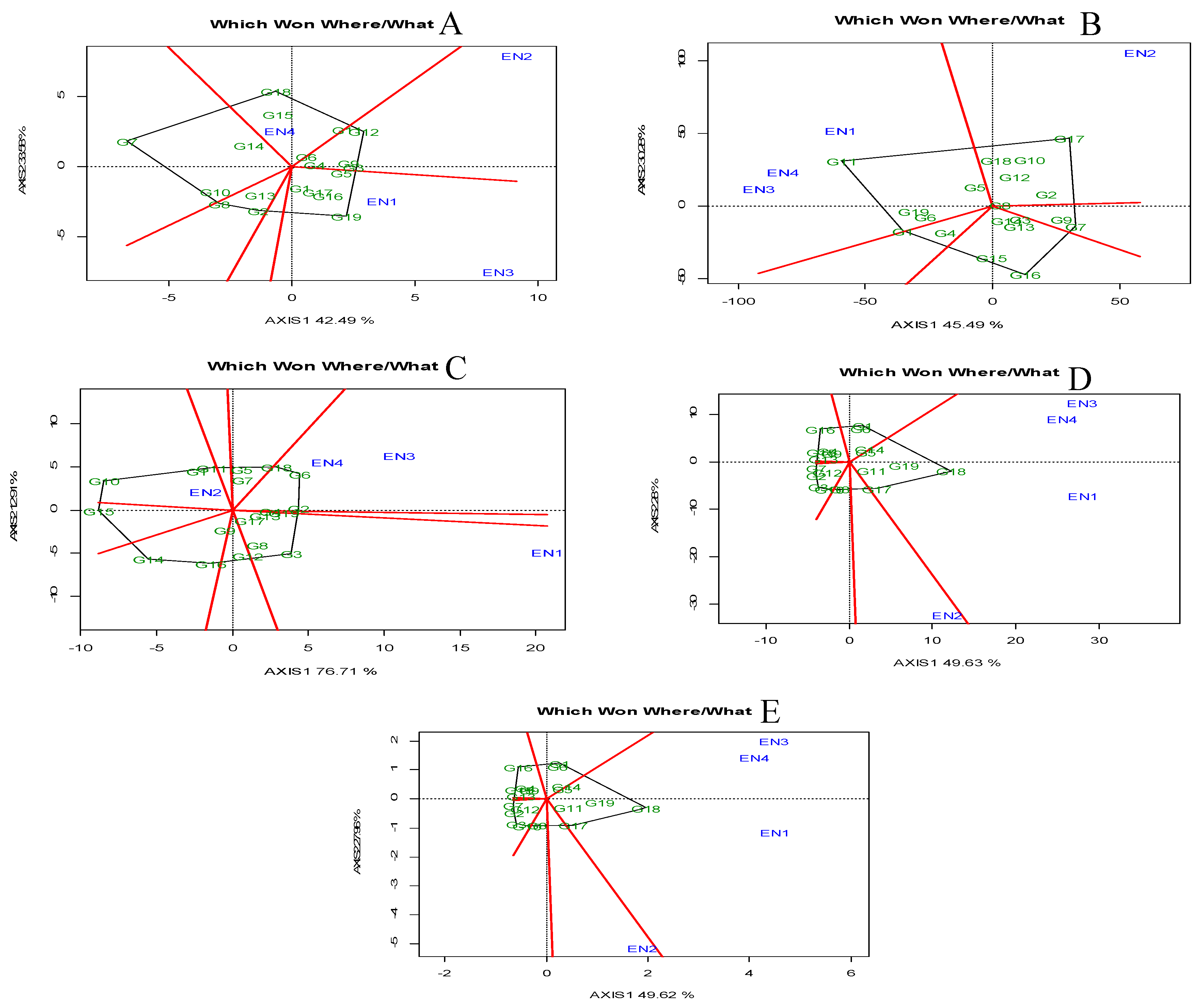
Figure 2.
GGE Biplot analyses for mean vs stability. Note: A=days to maturity, B=plant height, C=no. filled grains, D=total grains weight per hill, E=Yield per hectare.
Figure 2.
GGE Biplot analyses for mean vs stability. Note: A=days to maturity, B=plant height, C=no. filled grains, D=total grains weight per hill, E=Yield per hectare.
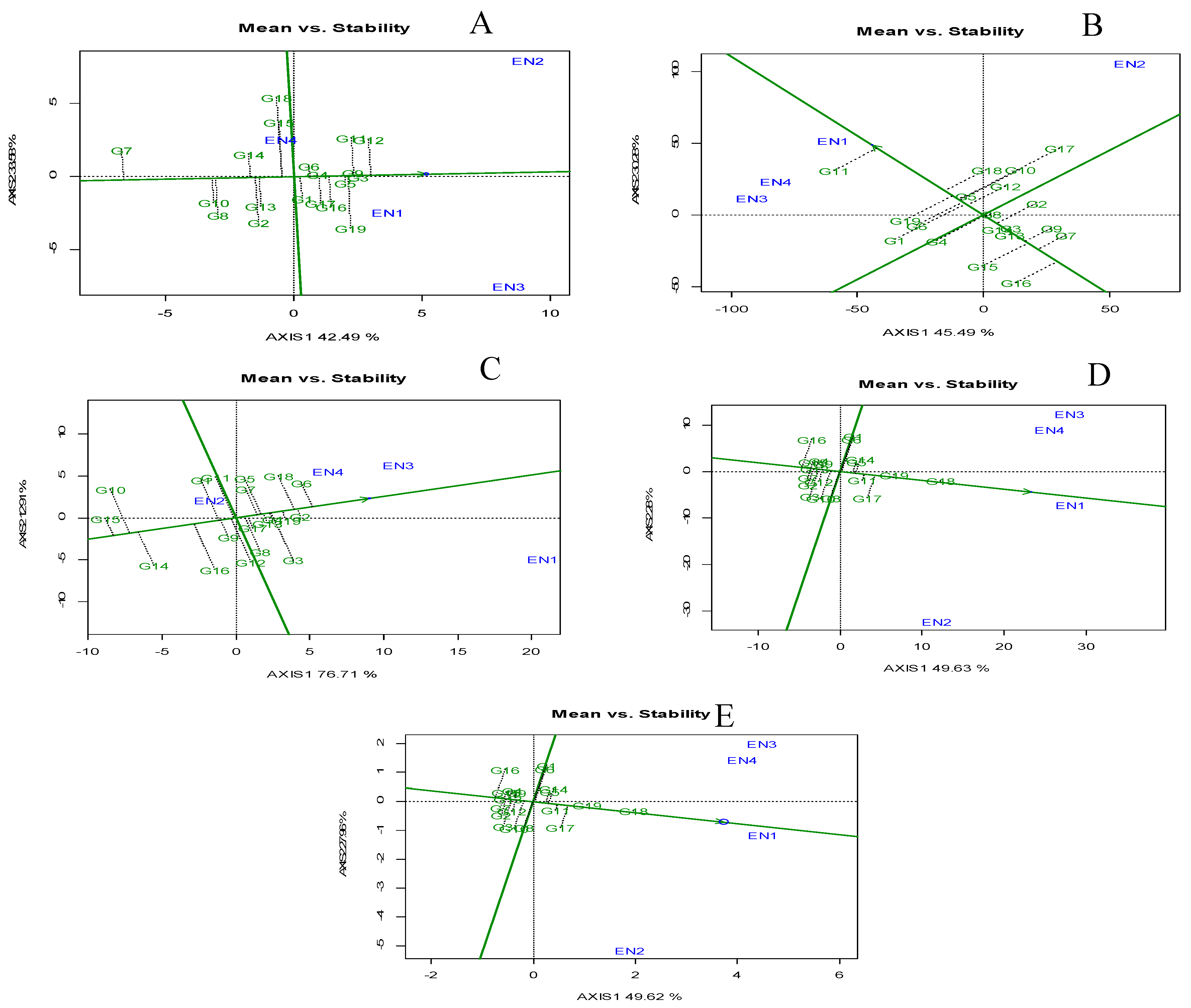
Figure 3.
GGE Biplot analyses for ranking genotypes. Note: A=days to maturity, B=plant height, C=no. filled grains, D=total grains weight per hill, E=Yield per hectare.
Figure 3.
GGE Biplot analyses for ranking genotypes. Note: A=days to maturity, B=plant height, C=no. filled grains, D=total grains weight per hill, E=Yield per hectare.
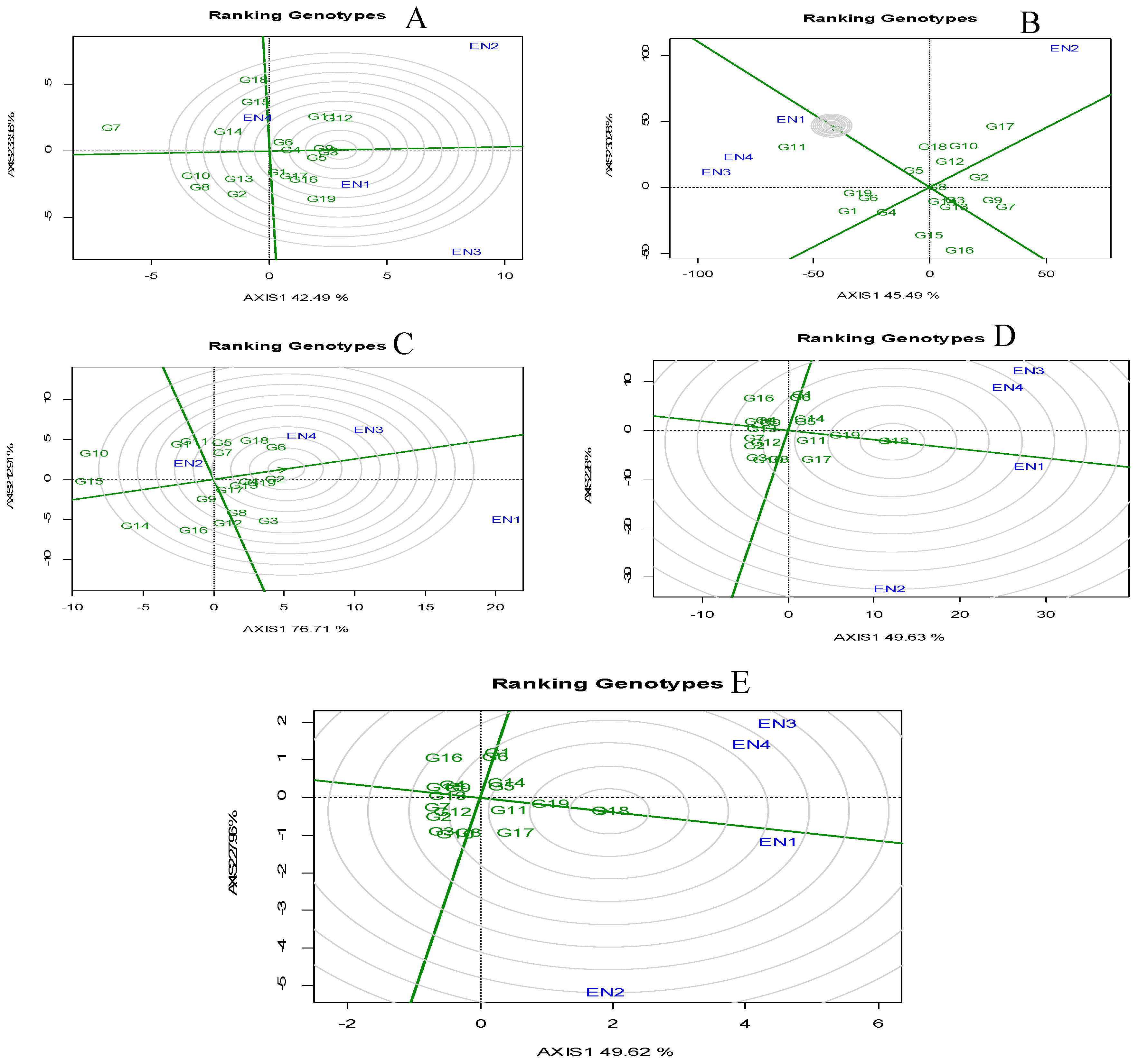
Figure 4.
GGE Biplot analyses for discriminative vs representative analysis. Note: A=days to maturity, B=plant height, C=no. filled grains, D=total grains weight per hill, E=Yield per hectare.
Figure 4.
GGE Biplot analyses for discriminative vs representative analysis. Note: A=days to maturity, B=plant height, C=no. filled grains, D=total grains weight per hill, E=Yield per hectare.
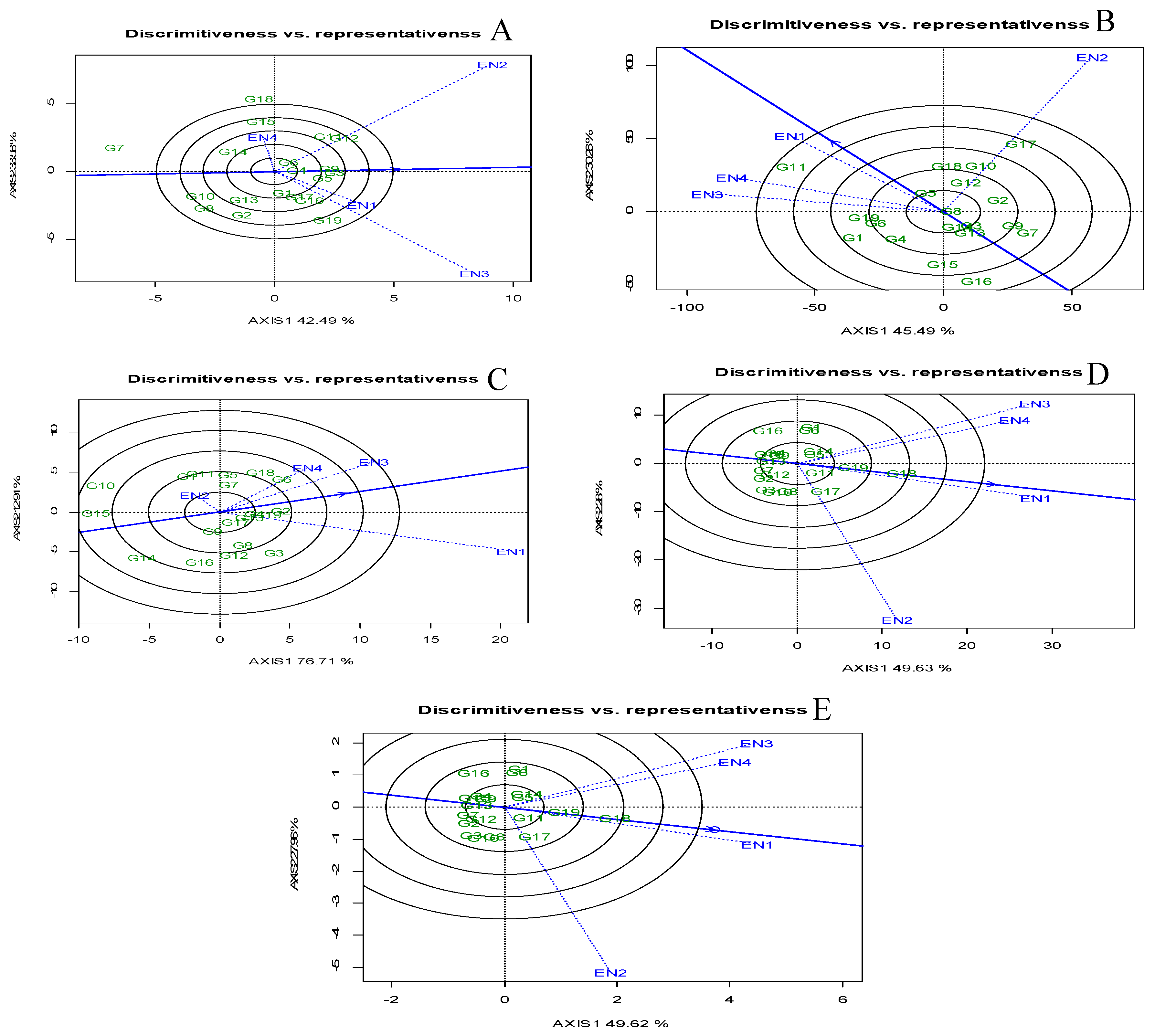
Figure 5.
GGE Biplot analyses for ranking environments. Note: A=days to maturity, B=plant height, C=no. filled grains, D=total grains weight per hill, E=Yield per hectare.
Figure 5.
GGE Biplot analyses for ranking environments. Note: A=days to maturity, B=plant height, C=no. filled grains, D=total grains weight per hill, E=Yield per hectare.
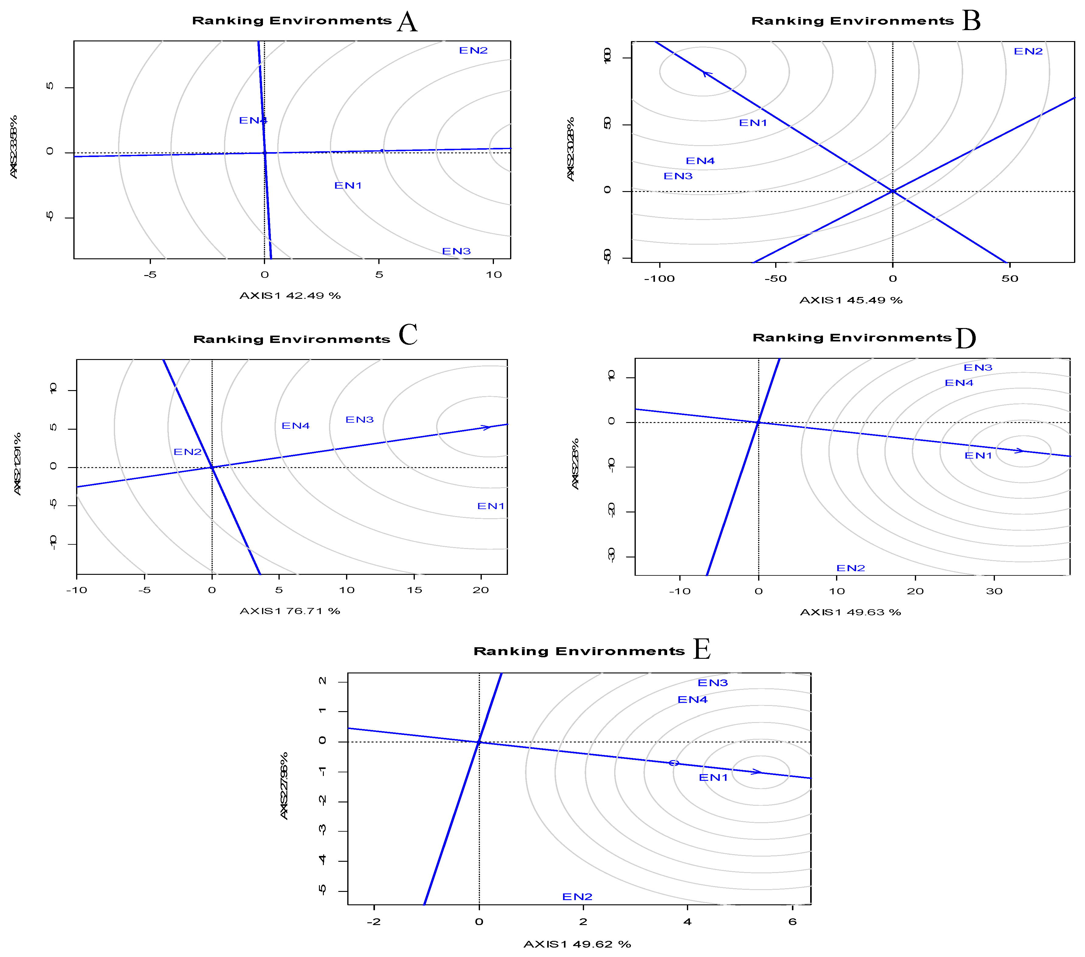
Figure 6.
GGE Biplot analyses for AMMI1. Note: A=days to maturity, B=plant height, C=no. filled grains, D=total grains weight per hill, E=Yield per hectare.
Figure 6.
GGE Biplot analyses for AMMI1. Note: A=days to maturity, B=plant height, C=no. filled grains, D=total grains weight per hill, E=Yield per hectare.
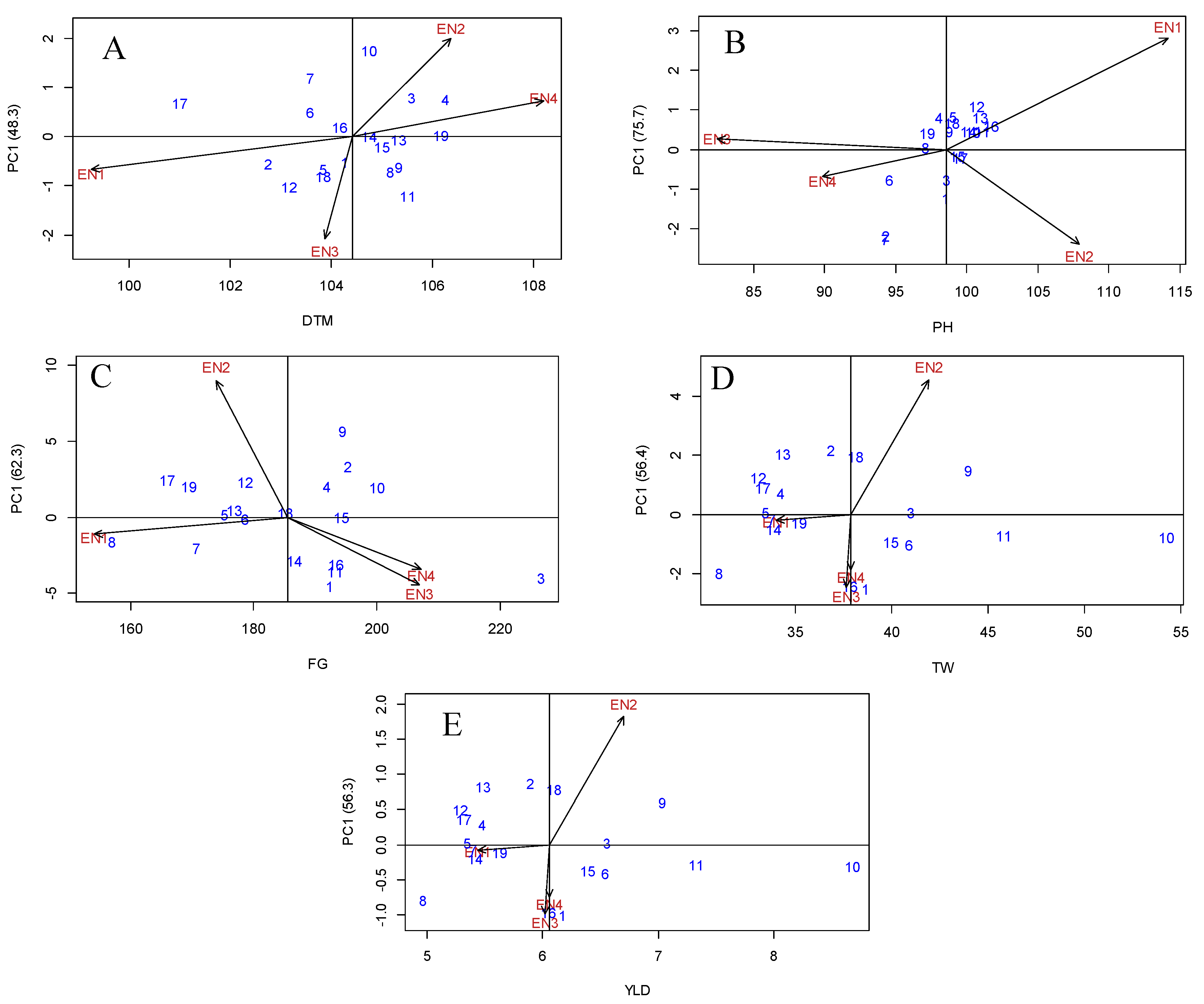

Table 1.
Response of the improved lines to rice blast pathotype 7.2.
| Improved line | Blast disease reaction after challenging with inoculum (scale: 0-5) |
Blast disease screening under protected glass house (scale: 0-9) |
|
|---|---|---|---|
| MARDI | UPM | ||
| 1 | MR | MR | MR |
| 2 | R | R | R |
| 3 | MR | R | MR |
| 4 | MR | MR | R |
| 5 | R | R | R |
| 6 | R | R | R |
| 7 | MR | MR | MR |
| 8 | R | R | R |
| 9 | R | MR | MR |
| 10 | R | R | R |
| 11 | R | R | R |
| 12 | MR | R | MR |
| 13 | R | R | R |
| 14 | R | R | R |
| 15 | MR | R | R |
| 16 | MR | MR | MR |
| 17 | R | R | R |
| 18 | R | R | R |
| MR219 | S | S | S |
| Pongsu Seribu 2 | R | R | R |
Note: R=resistant, MR=moderately resistant, S=susceptible.
Table 2.
Univariate stability analyses for days to maturity and plant height.
| Days to Maturity | Plant Height | |||||||||||
|---|---|---|---|---|---|---|---|---|---|---|---|---|
| G | M | bi | S2d | σi2 | Wi2 | YSi | M | bi | S2d | σi2 | Wi2 | YSi |
| 1 | 104.25 | 1.44 | 5.71 | 8.57 | 25.41 | 8 | 98.52 | 1.24 | 27.7 | 31.26 | 87.52 | 4 |
| 2 | 103.17 | 1.58* | 13.52* | 11.91 | 34.37 | 2 | 100.73 | 1.11 | 24.45 | 24.4 | 69.09 | 17 |
| 3 | 105.33 | 1.45 | 10.04 | 8.71 | 25.79 | 15 | 100.93 | 0.02 | 15.03 | 39.07* | 108.47 | 14 |
| 4 | 104.75 | 1.34 | 2.23 | 2.02 | 7.83 | 12 | 100.13 | 0.26 | 7.61 | 4.66 | 16.11 | 15 |
| 5 | 105 | 0.99 | 7.53* | 8.14 | 24.25 | 13 | 99.33 | 1.09 | 3.93 | 7.65 | 24.13 | 13 |
| 6 | 104.17 | 0.28 | 10.82 | 9.14 | 26.93 | 7 | 101.73 | 1.11 | 10.71 | 9.78 | 29.85 | 21 |
| 7 | 101 | -0.88** | 70.87** | 30.35* | 83.86 | -5 | 99.55 | 2.92 | 19.5 | 2.24 | 9.62 | 14 |
| 8 | 103.83 | 1.02 | 32.14** | 34.79** | 95.78 | -3 | 98.93 | 1.3 | 37.60* | 11 | 33.12 | 11 |
| 9 | 106.17 | 1.28 | 2.63 | 1.14 | 5.46 | 19 | 97.25 | 1.86 | 4.48 | 4.48 | 15.62 | 4 |
| 10 | 102.75 | 1.82* | 15.93 | 10.81 | 31.41 | 1 | 94.35 | 1.94 | 74.01 | 92.78*** | 252.64 | -8 |
| 11 | 105.58 | 1.58 | 7.12 | 13.25 | 37.97 | 18 | 98.61 | -0.65 | 9.34 | 12.98 | 38.44 | 9 |
| 12 | 106.25 | -0.75* | 24.88 | 9.34 | 27.48 | 20 | 98.05 | -0.38 | 12.55 | 13.36 | 39.45 | 5 |
| 13 | 103.83 | -0.18 | 12.58 | 6.68 | 20.34 | 6 | 99.04 | 1.52 | 22.53* | 21.39 | 61.02 | 12 |
| 14 | 103.58 | 0.37 | 10.19 | 4.53 | 14.57 | 4 | 94.57 | 1.31 | 12.65 | 13.84 | 40.76 | 1 |
| 15 | 103.58 | 1.91 | 17.36 | 20.14 | 56.46 | 2 | 94.28 | 0.66 | 99.42 | 103.05*** | 280.21 | -9 |
| 16 | 105.17 | 1.49 | 11.84 | 7.7 | 23.07 | 14 | 97.12 | 1.51 | 8.97 | 9.52 | 29.15 | 3 |
| 17 | 105.33 | 1.25 | 9.8 | 10.86 | 31.55 | 16 | 98.79 | 0.08 | 6.96 | 3.72 | 13.59 | 10 |
| 18 | 104.75 | 0.45 | 45.65** | 47.57** | 130.08 | 4 | 100.48 | 1.71 | 10.46 | 16.05 | 46.68 | 16 |
| MR219 | 105.5 | 1.89 | 25.66 | 43.18** | 118.3 | 9 | 101.1 | 0.4 | 7.7 | 12.32 | 36.67 | 19 |
Note: M=Means corrected by least squares; bi=Regression coefficient; σi2 =Shukla’s stability variance; Wi2 =Wrickle’s ecovalence; S2d =Deviation from regression; YSi =Kang stability statistics; *Significant difference (p<0.05), **Highly significant difference (p<0.01).
Table 3.
Univariate stability analyses for number of filled grains, total grains weight per hill and yield per hectare.
Table 3.
Univariate stability analyses for number of filled grains, total grains weight per hill and yield per hectare.
| Number of Filled Grains | Total Grains Weight per Hill | Yield per Hectare | ||||||||||||||||
| G | M | bi | S2d | σi2 | Wi2 | YSi | M | bi | S2d | σi2 | Wi2 | YSi | M | bi | S2d | σi2 | Wi2 | YSi |
| 1 | 192.33 | 0.42 | 2582.03 | 3117.45** | 8643.13 | 5 | 38.6 | 1.68 | 335.50* | 362.72** | 995.41 | 6 | 6.17 | 1.68 | 8.594* | 9.29** | 25.5 | 6 |
| 2 | 178.67 | -1.07* | 316.12 | 2412.97** | 6752.15 | -1 | 33.05 | 0.82 | 116.67* | 121.93 | 349.1 | 1 | 5.29 | 0.82 | 2.987* | 3.12 | 8.94 | 1 |
| 3 | 176.83 | 0.44 | 187.71 | -22.94*** | 213.68 | -3 | 34.3 | -0.26 | 240.83 | 178.02 | 499.65 | 7 | 5.49 | -0.26 | 6.161 | 4.55 | 12.77 | 7 |
| 4 | 186.58 | 0.26 | 851.23 | 2319.33* | 6500.81 | 7 | 33.83 | -1.36* | 59.4 | 1.18 | 24.97 | 5 | 5.41 | -1.36* | 1.52 | 0.03 | 0.64 | 5 |
| 5 | 194.25 | 2.13 | 525.26 | 136.01 | 640.31 | 16 | 39.95 | 1.08 | 33.68 | 25.56 | 90.42 | 15 | 6.39 | 1.08 | 0.857 | 0.65 | 2.3 | 15 |
| 6 | 193.42 | 0.59 | 1053.53 | 1327.56 | 3838.7 | 13 | 37.8 | 1.29 | 191.76* | 232.00* | 644.53 | 6 | 6.05 | 1.29 | 4.912* | 5.93* | 16.48 | 6 |
| 7 | 165.92 | 0.24 | 1403.66** | 1326.01 | 3834.53 | -1 | 33.27 | 1.19 | 41.93 | 45.4 | 143.66 | 2 | 5.32 | 1.19 | 1.071 | 1.16 | 3.67 | 2 |
| 8 | 185.08 | 2.31 | 534.49 | -34.99*** | 181.33 | 0 | 38.12 | 1.72 | 84.26 | 180.33 | 505.85 | 13 | 6.1 | 1.72 | 2.152 | 4.61 | 12.93 | 13 |
| 9 | 169.42 | 2.5 | 1160.16 | 623.56 | 1949.02 | 2 | 35.16 | 2.27 | 47.88 | 62.25 | 188.89 | 8 | 5.63 | 2.27 | 1.225 | 1.59 | 4.83 | 8 |
| 10 | 195.33 | 0.83 | 1774.89* | 1931.61* | 5460.08 | 14 | 36.82 | -1.61* | 177.6 | 259.71* | 718.92 | 5 | 5.89 | -1.61* | 4.549 | 6.65* | 18.4 | 5 |
| 11 | 226.58 | 1.78 | 952.77 | 2761.39** | 7687.4 | 14 | 41 | 2.53 | 190.99 | 170.18 | 478.6 | 17 | 6.56 | 2.52 | 4.89 | 4.36 | 12.27 | 17 |
| 12 | 191.92 | 2.72* | 1445.97* | 624.24 | 1950.84 | 12 | 34.21 | 1.23 | 212.32 | 198.77 | 555.33 | 4 | 5.47 | 1.23 | 5.439 | 5.09 | 14.22 | 4 |
| 13 | 175.17 | -0.45 | 785.11 | 108.49 | 566.45 | 4 | 33.44 | 0.41 | 6.41 | 2.67 | 28.97 | 3 | 5.35 | 0.41 | 0.165 | 0.07 | 0.74 | 3 |
| 14 | 178.67 | 2.68** | 599.73** | -100.76*** | 4.78 | -2 | 40.91 | 2.36 | 105.15 | 107.79 | 311.12 | 16 | 6.55 | 2.36 | 2.68 | 2.75 | 7.94 | 16 |
| 15 | 170.58 | -0.29 | 1037.82 | 2101.41* | 5915.86 | -1 | 33.76 | 0.36 | 224.60* | 147.03 | 416.46 | 4 | 5.4 | 0.35 | 5.758* | 3.77 | 10.67 | 4 |
| 16 | 156.92 | 2.22* | 874.24* | 480.56 | 1565.16 | -1 | 31.01 | 1.49 | 190.98 | 205.47 | 573.33 | -2 | 4.96 | 1.49 | 4.895 | 5.27 | 14.7 | -2 |
| 17 | 194.42 | 0.45 | 2879.48 | 5160.03*** | 14125.9 | 9 | 43.95 | 1.5 | 39.77 | 105.93 | 306.13 | 18 | 7.03 | 1.5 | 1.018 | 2.71 | 7.82 | 18 |
| 18 | 199.92 | 1.66 | 652.73 | 571.39 | 1808.98 | 19 | 54.23 | 1.34 | 28.18 | 19.83 | 75.02 | 22 | 8.68 | 1.34 | 0.72 | 0.51 | 1.92 | 22 |
| MR219 | 193.17 | -0.43 | 5522.54* | 8277.59*** | 22494 | 6 | 45.79 | 0.98 | 107.7 | 196.34 | 548.81 | 18 | 7.33 | 0.98 | 2.757 | 5.03 | 14.06 | 18 |
Note: M=Means corrected by least squares; bi=Regression coefficient; σi2 =Shukla’s stability variance; Wi2 =Wrickle’s ecovalence; S2d =Deviation from regression; YSi =Kang stability statistics.
Table 4.
Mean square for combined analysis of variance (ANOVA) for traits assessed over four environments.
Table 4.
Mean square for combined analysis of variance (ANOVA) for traits assessed over four environments.
| S.O.V | DF | DTM | PH | FG | TGW | YLD | |||||
|---|---|---|---|---|---|---|---|---|---|---|---|
| MS | TSS (%) | MS | TSS (%) | MS | TSS (%) | MS | TSS (%) | MS | TSS (%) | ||
| Blocks (environment) | 8 | 133.93** | 12.95 | 127.44** | 0.99 | 1791.21** | 3.90 | 449.08** | 27.27 | 11.49** | 27.28 |
| Genotypes (G) | 18 | 19.96ns | 1.93 | 60.67** | 0.47 | 2877.37ns | 6.27 | 380.11** | 23.09 | 9.73** | 23.10 |
| Environments (E) | 3 | 856.91** | 82.84 | 12680.89** | 98.27 | 38887.19** | 84.71 | 594.18** | 36.09 | 15.19** | 36.06 |
| G×E | 54 | 15.20** | 1.47 | 22.82** | 0.18 | 1743.21** | 3.80 | 138.06** | 8.38 | 3.53** | 8.38 |
| Error | 144 | 8.41 | 0.81 | 12.11 | 0.09 | 608.58 | 1.32 | 85.08 | 5.17 | 2.18 | 5.18 |
Note: *significant at p<0.05, **highly significant at p<0.01, ns: not significant at p>0.05, S.O.V: Source of variation, DF: Degree of freedom, MS: Mean square, TSS: Total sum of square, DTM: Days to maturity, PH: Plant height, FG: Number of filled grains per panicle, TGW: Total grain weight, YLD: Yield per hectare.
Table 5.
Correlation coefficients for agronomic and univariate stability traits.
| Variable | M | bi | σi2 | Wi2 | S2d | YSi | |
|---|---|---|---|---|---|---|---|
| Days to maturity | M | 1 | |||||
| bi | -0.10 | 1 | |||||
| σi2 | 0.16 | -0.21 | 1 | ||||
| Wi2 | 0.16 | -0.21 | 1.00** | 1 | |||
| S2d | 0.39 | -0.37 | 0.74** | 0.74** | 1 | ||
| YSi | 0.93*** | -0.10 | 0.42 | 0.42 | 0.60** | 1 | |
| Plant height | M | 1 | |||||
| bi | -0.39 | 1 | |||||
| σi2 | 0.20 | 0.03 | 1 | ||||
| Wi2 | 0.20 | 0.03 | 1.00** | 1 | |||
| S2d | 0.24 | -0.14 | 0.72** | 0.72** | 1 | ||
| YSi | 0.98** | -0.32 | 0.26 | 0.26 | 0.28 | 1 | |
| Number of filled grains | M | 1 | |||||
| bi | -0.21 | 1 | |||||
| σi2 | -0.40 | 0.14 | 1 | ||||
| Wi2 | -0.40 | 0.14 | 1.00** | 1 | |||
| S2d | -0.20 | 0.17 | 0.66** | 0.66** | 1 | ||
| YSi | 0.85** | -0.18 | -0.31 | -0.31 | -0.29 | 1 | |
| Total weight of grains | M | 1 | |||||
| bi | 0.24 | 1 | |||||
| σi2 | -0.03 | -0.16 | 1 | ||||
| Wi2 | -0.03 | -0.16 | 1.00** | 1 | |||
| S2d | 0.16 | -0.17 | 0.79** | 0.79** | 1 | ||
| YSi | 0.96** | 0.28 | 0.13 | 0.13 | 0.25 | 1 | |
| Yield per hectare | M | 1 | |||||
| bi | 0.24 | 1 | |||||
| σi2 | -0.03 | -0.16 | 1 | ||||
| Wi2 | -0.03 | -0.16 | 1.00** | 1 | |||
| S2d | 0.19 | -0.16 | 0.80** | 0.80** | 1 | ||
| YSi | 0.96** | 0.28 | 0.13 | 0.13 | 0.27 | 1 |
Note: M=Means corrected by least squares; bi=Regression coefficient; σi2 =Shukla’s stability variance; Wi2 =Wrickle’s ecovalence; S2d =Deviation from regression; YSi =Kang stability statistics.
Table 6.
Description on agronomic and morphological traits.
| Trait | Abbreviation | Unit | Description |
|---|---|---|---|
| Days to flowering | DTF | Number | Count the days from transplanting the seedlings in the field to the flowering stage |
| Days to maturity | DTM | Number | Count the days from transplanting the seedlings in the field to the maturing stage |
| Plant height | PH | cm | Measure from the base to the peak of top most panicle (awns eliminated) |
| Tillers per hill | NTH | Number | Amount of all tiller in each plant |
| Panicles per hill | NPH | Number | Total number of panicles for each plant |
| Panicle length | PL | cm | Measure from the panicle base (node below the lowest branch on panicle) to the tip of the last spikelet |
| Filled grains per panicle | FG | Number | Amount of filled (solid) grains |
| Unfilled grains per panicle | UFG | Number | Amount of unfilled (chaffy) grains |
| Total grains per panicle | TG | Number | The total amount of grains per panicle |
| Percentage of filled grains | PFG | Percentage |
Amount of filled grains × 100 Total grains |
| 1000-grain weight | TGW | gram | Weight of one thousand full-filled grains for each plant |
| Total weight of grains per hill | TW | gram | Weight of all filled grains for each plant |
| Yield | YLD | t/ha | Average total weight of grains per plant multiply number of plants per square meter divided by 100 |
Disclaimer/Publisher’s Note: The statements, opinions and data contained in all publications are solely those of the individual author(s) and contributor(s) and not of MDPI and/or the editor(s). MDPI and/or the editor(s) disclaim responsibility for any injury to people or property resulting from any ideas, methods, instructions or products referred to in the content. |
© 2025 by the authors. Licensee MDPI, Basel, Switzerland. This article is an open access article distributed under the terms and conditions of the Creative Commons Attribution (CC BY) license (http://creativecommons.org/licenses/by/4.0/).
Copyright: This open access article is published under a Creative Commons CC BY 4.0 license, which permit the free download, distribution, and reuse, provided that the author and preprint are cited in any reuse.


