
Submitted:
04 October 2025
Posted:
06 October 2025
Read the latest preprint version here
Abstract
We present a symmetry-based framework for torsionful gravity in the Palatini formulation that ensures luminal gravitational waves (c_T = 1) without parameter tuning and without extra propagating modes. The organizing principle is a scalar PT projector on observable scalar densities, paired with projective symmetry implemented by a Stueckelberg compensator epsilon(x) that enters only through the invariant trace T_mu − partial_mu epsilon. Within a two-derivative, parity-even posture (A1–A5) we establish three conditional results: (C1) pure-trace alignment, fixing torsion by partial_mu epsilon while axial and traceless irreps vanish; (C2) three-route bulk equivalence, showing that determinant/rank-one, closed-metric, and PT-even CS+ constructions share the same quadratic bulk up to improvement currents; and (C3) coefficient locking, which removes TT–non-TT mixing and enforces K = G, hence c_T = 1 exactly at quadratic order with only two tensor degrees of freedom. The leading parity-even NLO correction is unique and predicts delta c_T^2(k) = b k^2 / Lambda^2 for k << Lambda. We propose falsifiable diagnostics: a quadratic-slope test for delta c_T^2 across frequency bands, and a route-equality/flux-ratio null (Delta A_* -> 0) in the strict spurion limit. A projectively invariant Stueckelberg completion with m_T -> infinity (or a Lagrange current enforcing T_mu − partial_mu epsilon) explains the gradient-only appearance of epsilon and justifies treating it as nondynamical at low energies; residual dynamics would yield controlled, testable deviations. All figures and reductions are reproducible from a public code release. The framework delineates a symmetry-selected, data-facing sector of torsionful modified gravity consistent with multimessenger bounds.
Keywords:
Palatini formalism
; PT-even projector
; pure-trace torsion
; trace-lock posture
; Nieh–Yan invariant
; parity-even Chern–Simons projection
; rank-one determinant (ROD)
; closed-metric deformation
; coefficient locking
; three-chain equivalence
; gravitational-wave tensor modes
; exact luminality (c_T=1)
1. Introduction
Motivation and context. Multimessenger observations (e.g., GW170817/GRB170817A) enforce luminal gravitational waves today, severely constraining tensor-sector deviations from GR and motivating symmetry-driven routes that deliver without fine tuning. At the same time, long-standing work in Einstein–Cartan/metric–affine (EC/MAG) geometry shows how torsion and non-metricity can be organized consistently, while Palatini-type modified gravity (notably Palatini ) has faced well-documented pitfalls when matter is included. This paper asks a focused question: Can one formulate a first-order (Palatini) framework whose observable sector is (i) -even by construction, (ii) closed at quadratic order with at most one derivative per building block, (iii) exactly luminal for tensor modes by a structural identity, and (iv) free of extra propagating degrees of freedom?
Posture and scope. We work with independent vierbein and a metric-compatible spin connection , and we enforce a scalar projector on observable scalar densities. On oriented -manifolds, the combined preserves orientation and commutes with the Hodge dual, so scalar densities can be projected to -even pieces; -odd scalar densities are discarded as unobservable (real) expectation values. An internal phase (Stueckelberg compensator) enters the observed sector only through its gradient; we adopt a spurion limit (not varied) at quadratic order. Global assumptions A1–A6 (domain/measure; ; projection/variation commutes on scalar densities; boundary/topology posture with Nieh–Yan as boundary; two-derivative closure) delimit the posture (Section 2). A quick notation table appears in Section 2.3 for ease of reference.
Projective symmetry and the invariant trace. Palatini geometry admits projective shifts
To keep the projected observable sector invariant, we introduce a compensator whose gradient shifts as and work with the projectively invariant trace
Within the two-derivative posture, all observables depend on only through via .
Quadratic basis (one-derivative per factor). At quadratic order, the projected, real invariants we use are
together with improvement currents that are pure boundary under A4–A5.
- Main results (at a glance).
|
All three results hold at quadratic order, within A1–A6 and the scalar- observable sector. (C1) Conditional Palatini– uniqueness under trace-lock (A6). Algebraic torsion consistent with the scalar projector is uniquely pure trace and aligned with : |
|
(C2) Three-chain bulk equivalence (mod boundary). After projection and using C1, three constructive routes collapse to the same bulk quadratic piece: |
|
(C3) Coefficient locking ⇒ exact luminality. Eliminating TT–nonTT mixing fixes a unique weight so that |
Plain-language gist (reader’s guide). What we do: (i) keep only -even scalar observables; (ii) use a compensator so only the trace of torsion in the invariant combination matters; (iii) show three seemingly different quadratic routes give the same bulk physics (C2); (iv) choose coefficients once and for all to kill mixing, which forces (C3). What you can test: a unique next-to-leading dispersion
for multi-band GW data (PTA/LISA/LVK), detailed in Section 9; if a slope is absent where EFT is valid, this posture is disfavored.
Falsifiable diagnostics (paper-level). Within A1–A6, any of the following falsifies the framework at quadratic order:
- (C1 fails) Robust axial/traceless torsion signals in observables, or inability to realize , with .
- (C2 fails) Disagreement of bulk coefficients among rank-one determinant (ROD), closed-metric (CM), and -even CS/Nieh–Yan routes once improvements are accounted for; the flux ratio on admissible domains.
- (C3 fails) No coefficient choice achieves , or persists after locking on admissible patches.
Positioning relative to prior lines. In EC/MAG, axial/traceless torsion can propagate; here they are algebraically removed in the analyzed sector (C1). Parity-odd (dynamical) Chern–Simons gravity ties tensor effects to a pseudo-scalar; our -projected, even-parity sector achieves luminality by an equal-coefficient identity (C3), modulo improvements. Nieh–Yan contributes only boundary counterterms under A5 and does not alter bulk equations. The three-chain collapse (C2) is a rank-one, quadratic statement: ROD, CM, and the -even CS/Nieh–Yan shadow share the same bulk piece , differing only by .
Organization and stability notes. Section 2 fixes A1–A6 and the scalar projector; Section 3 and Section 4 prove C1; Section 5 proves C2 and defines flux-ratio diagnostics; Section 6 and Section 7 implement locking and prove (C3), also giving representatives; matter couplings and the data-facing NLO piece appear in Section 8 and Section 9. Locking is stable on generic patches: the mixing determinant scales as with , so rank loss occurs only on the measure-zero set .
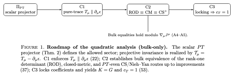
Figure 1.
Roadmap of the quadratic analysis (bulk-only). The scalar projector (Thm. 2) defines the allowed sector; projective invariance is realized by . C1 enforces (22); C2 establishes bulk equivalence of the rank-one determinant (ROD), closed-metric, and -even CS/Nieh–Yan routes up to improvements (37); C3 locks coefficients and yields and (53).
2. Global Assumptions & the Scalar Projector
We work on an oriented -dimensional spacetime with independent vierbein and a metric-compatible spin connection (Palatini posture). Greek indices are spacetime; Latin are Lorentz-frame indices with . Torsion and curvature are
Observable scalar densities are mapped to a real, -even sector by a projector defined below. The internal phase is a spurion: it enters observables only via and is not varied in the posture adopted here.
Physical Motivation for the Scalar Projector
We restrict observable scalar densities to the -even, real sector for two reasons: (i) on oriented -manifolds the combined preserves orientation and commutes with the Hodge dual ∗, so the Levi–Civita density (weight ) is -even; (ii) by the anti-linearity of T, expectation values of -odd scalar densities are purely imaginary and thus unobservable as real densities. We therefore average a scalar with its image and take the real part, Equation (8). This is a posture on observables, not on fields. The commutation Lemma 1 and a minimal counterexample with render the posture directly checkable in our setup.
2.1. Projective Symmetry and the Stueckelberg Spurion
Palatini geometry admits a projective symmetry under which the connection shifts as
To maintain invariance of the -even observable sector after imposing the scalar projector, we introduce a Stueckelberg compensator whose gradient transforms as
and we work with the projectively invariant trace combination
Within the two–derivative truncation adopted here, we take the spurion limit in which dynamical fluctuations of are frozen; thus the allowed -even scalar sector depends on only through . Combined with A1–A5, this ensures that the scalar projector commutes with variation on scalar densities (Lemma 1). In Section 3 we enumerate the resulting quadratic basis, and in Section 4, Section 5, Section 6 and Section 7 we show how (C1) aligns with so that at the level analyzed.
Assumption Posture at a Glance (A1–A6; observable scalars are -even and real).
|
Sufficient conditions for A1. On oriented Lorentzian patches with the standard measure and -invariant boundaries (compact or AF/FRW fall-offs), the pullback by preserves both the integration domain and the measure, hence for scalar densities.
Sufficient conditions for A2. If preserves the chosen orientation and the metric used for index operations, then commutes with the Hodge dual on forms: .
Action of on Densities
Let act as standard discrete isometries; T is anti-linear (complex conjugation). On oriented -manifolds, the combined preserves orientation, so for the Levi–Civita density (weight ) we have
Assumption A2 implies . Consequently, a scalar of the form is -even iff X is -even.
2.2. Scalar Projector: Definition and Basic Properties
The combined acts anti-linearly on complex-valued densities (complex conjugation accompanies time reversal). On scalar densities we define
Self-adjointness on real scalars. Using A1 and ,
Lemma 1
(Project–vary commutation on scalar densities). Let act on complex-valued scalar densities with A1 (PT-invariant domain/measure) and A4 (fall-offs) imposed. If the spurion ϵ is non-variational and variations act only on with compact support or admissible fall-offs, then and is self-adjoint on real scalars.
Proof.
Anti-linearity of T affects only ; variations here are real-linear on , and is fixed. With A1, implies on real scalars (self-adjointness). Then , where boundary terms vanish by A4. □
Function-analytic hypotheses and a minimal counterexample. Assume (scalar densities), or with A4 fall-offs, and the spurion is non-variational. Since T is anti-linear (complex conjugation), acts as . Under these conditions is real-linear and .
If, however, is varied, the commutation may fail. Let with a real . Then (purely -odd), but when . Hence . This shows why we hold fixed (spurion posture).
Admissible variation space. Variations act on with compact support or with A4 fall-offs: on AF patches with ; on FRW slices, , for some . The spurion is nondynamical (no variation) and T’s anti-linearity only sends . Under these conditions is real-linear and boundary fluxes vanish, so holds term-by-term.
Variational domain for identity. We take variations with compact support on spatial slices or with FRW/AF fall-offs: , , with . Then and
2.3. Quick Tables (Projection-Ready)
Objects. (Signs indicate intrinsic P/T parities; T is anti-linear.)
| Object | P | T | Note |
| + | + | vierbein (metric from its square) | |
| + | − | spin connection | |
| + | − | torsion 2-form components | |
| + | + | curvature 2-form components | |
| (spurion) | + | − | enters observables via only |
| − | + | flips under P; T anti-linear | |
| − | − | pseudo-density (weight ); ; by A2 |
Scalar monomials and the projector.
| Monomial | ||
| even | survives; real by definition | |
| even | survives; real under projection | |
| even even | kept iff X is -even; else projected out | |
| even | survives pre-lock; reduces to after C1/trace-lock | |
| (vector density) | — (total deriv.) | boundary-only under A4; unaffected except taking real part |
Notation Quick Reference (Projected, Real Scalars; Sign-Compensated Scheme)
|
Projected spurion scalar. |
2.4. Selection Rules Under the Scalar Projector
Theorem 2
(Selection rules). Under A1–A5 and (A2), for any complex scalar density ,
In particular, for admissible tensors X,
- Sketch. By definition (8), averages an object with its image and then takes the real part. With A1, ensures self-adjointness (9) on real scalars. A2 implies preserves orientation and commutes with ∗. Since the Levi–Civita density is -even while T is anti-linear, inherits the parity of X, yielding the conditional statement above. Products such as are -even (see the quick table), hence survive the projector; their later reduction to uses the trace-lock/C1 map (Section 3 and Section 4).
Roadmap and Where Each Assumption Enters
The definitions and rules above are the only projectors/boundary tools used later. In particular:
- Section 3 (allowed sector/closure): we enumerate all -even quadratic monomials with at most one derivative per building block. Pre-lock the basis includes , , and . Post-lock (trace-lock or C1) maps .
- Section 4 (C1): A3 enables project-then-vary in the Palatini connection equation; A2/A5 prevent hidden pseudo-scalar contaminations; A4 controls improvements.
- Section 5 (C2, scheme): A5 ( boundary) and A1/A4 underwrite the equality of route-wise bulk pieces and flux-ratio diagnostics, all written with the sign-compensated invariant .
Boundary/Topology Posture And Fall-Offs (Pointer)
Assumption A4 is realized either by compact -invariant domains with vanishing flux or by standard asymptotically flat/FRW fall-offs; the explicit statements and the symplectic-flux check are compiled in Appendix A (boundary notes therein). We exclude torsion defects and multi-valued patches that would violate the projector’s scalar posture.
3. Palatini Setting and the Allowed -Even Scalar Sector
We work in the Palatini posture with independent vierbein and a metric-compatible spin connection . Throughout this section the global assumptions A1–A6 and the scalar projector of Section 2 are in force, together with the selection rules of Theorem 2. All scalar densities are implicitly projected, hence real and -even. We also retain the two–derivative truncation and the spurion posture: the internal phase enters observables only through its gradient and is not varied.
3.1. Projectively Invariant Starting Point
As reviewed in Section 2.1, Palatini geometry admits a projective symmetry under which the torsion trace shifts and is compensated by the gradient of . We therefore formulate the allowed sector in terms of the projectively invariant combination
Within the spurion limit (two–derivative regime; frozen dynamics), PT–even observables depend on only through . In Section 4 we will show that the Palatini equations together with the trace-lock posture (C1) align with , effectively setting on admissible patches. The present section establishes the corresponding operator basis and its closure properties before and after this lock.
3.2. Normalized Spurion Direction and Canonical Rank-One Tensor
It is convenient to record the projected spurion scalar and the normalized direction of :
From we define a dimensionless, traceless rank-one tensor
The (dimension-one) torsion trace scale along will be denoted
When we work on patches and extend by continuity via a smooth regulator , . We emphasize the notational distinction: is the projectively invariant trace vector (13), while in (15) is a traceless rank-one matrix built from .
3.3. What the Projector Allows (Pre- vs. Post-Lock)
By Theorem 2 and the parity assignments of Section 2, the following quadratic monomials with at most one derivative per building block are -even and thus survive the scalar projector:
The mixed bilinear is therefore independent pre-lock.1 Once the Palatini– uniqueness map (C1; Section 4) or, equivalently, the trace lock is enforced,
and the mixed bilinear collapses to the spurion scalar.
For later reference we summarize the fate of the monomials:
| Monomial | Projected fate (pre-lock → post-lock) | |
| even | survives → survives | |
| even | survives → survives | |
| even | survives, independent → | |
| — | improvement → improvement |
3.4. Two-stage closure at one-derivative order
Allowing at most one derivative per building block and working to quadratic order, the projected, real, -even scalar sector closes in two stages:
The self-adjointness of on real scalars (9) and A4 (boundary posture) justify the integration-by-parts steps implicit in (18).
Lemma 3
(Two-stage closure). Under A1–A5, any -even quadratic scalar density with at most one derivative per factor satisfies
for some real constants and an improvement current . After enforcing ,
with and a (possibly shifted) improvement current .
- Sketch. Enumerate quadratic monomials; Theorem 2 removes only -odd combinations. The three even monomials span the pre-lock space up to improvements; A1 and A4 ensure the projector’s self-adjointness and the harmlessness of boundary terms. The lock gives the post-lock reduction.
3.5. Action skeleton (pre- and post-lock) and invariant notation
A minimal bulk skeleton compatible with the closure is
with . After the lock (C1) this becomes
so the sole effect of at this order is a renormalization of the coefficient.
For compactness we also introduce the torsion quadratic invariant (projected, real)
and, when convenient, its sign-compensated version . In Section 4 we will show that C1 implies , so that the post-lock basis may be written as .
Order of Operations and Consistency
The scalar projector acts at the level of densities; by Lemma 1 (Section 2) we may project then vary or vary then project on scalar densities. The trace lock is an algebraic enforcement at the level of equations of motion (or via a Lagrange current); it is not a projection and introduces no new canonical pairs under A4. Accordingly, the pipeline for the quadratic sector is:
Paper-level null test. On any admissible background with A4 fall-offs, every projected, -even quadratic density with at most one derivative per building block reduces pre-lock to up to a total derivative, and post-lock to up to a total derivative. An explicit constructive reduction appears in the Appendix.
4. Uniqueness Theorem (C1)
- Within A1–A6 and the scalar- observable sector, at quadratic order with at most one derivative per building block, the Palatini connection equations fix algebraic torsion to be pure trace aligned with the spurion gradient. Equivalently,
Figure 2.
Irreducible torsion content at quadratic order (log–log view). Ratios of projected scalar strengths comparing the pure-trace block against the axial and traceless blocks, shown as trace/axial and trace/tensor on logarithmic axes. The Palatini algebraicity (Section 4.2) and the projector drive axial and traceless pieces to zero, leaving the pure-trace map (22) as the unique survivor. [nb: fig_c1_pure_trace.py].
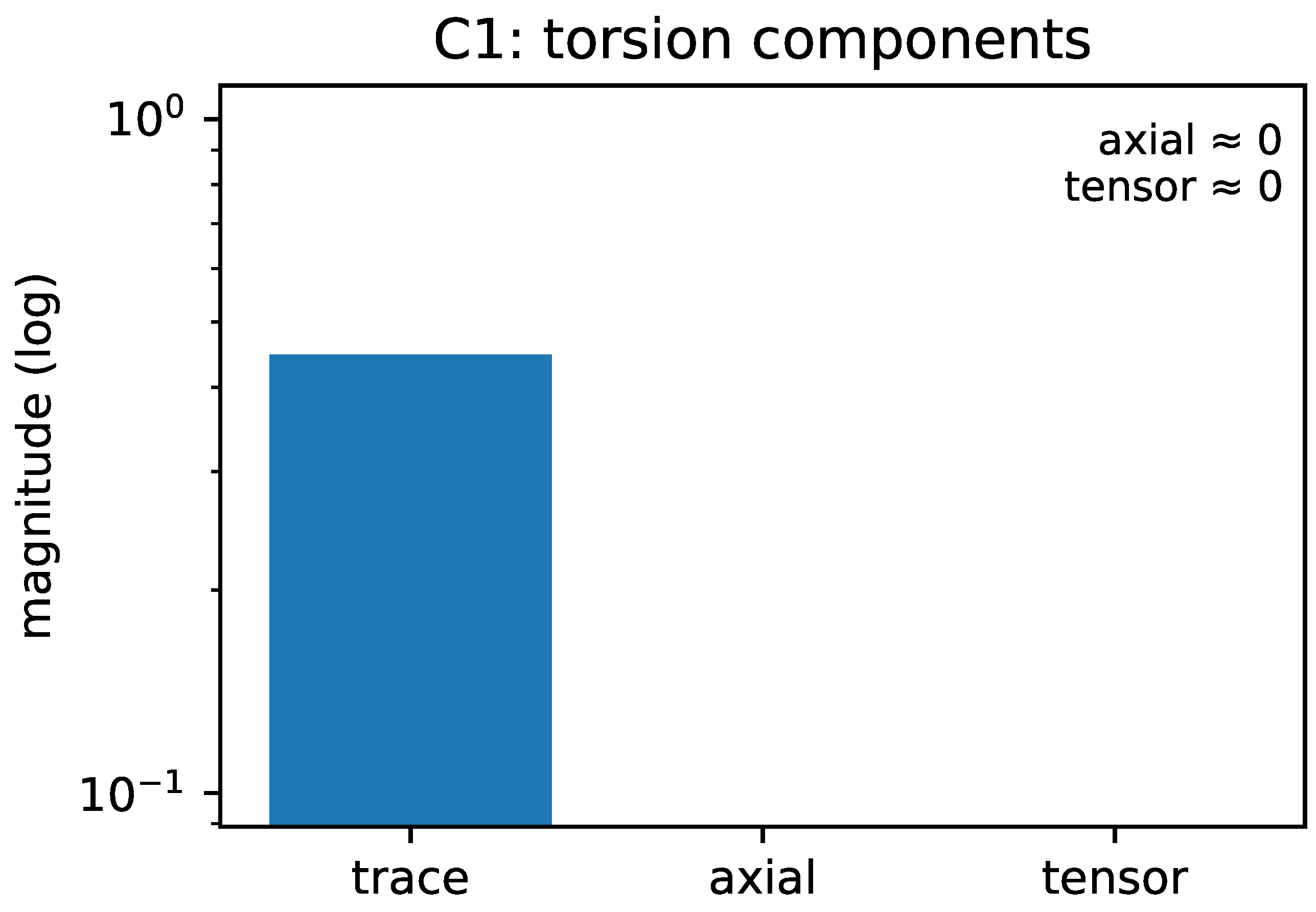
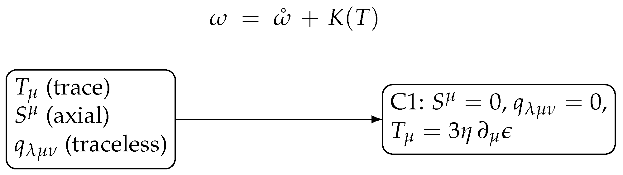
Figure 3.
Connection decomposition and the C1 map. Top: the Levi–Civita/contorsion split . Bottom: torsion irreps and the C1 alignment , , (22), which implies (23).
4.1. Most General Local Linear Ansatz (One Derivative)
At the derivative order relevant for the quadratic analysis, the only covector available is and the invariant tensors are and . The most general Lorentz-covariant linear ansatz is therefore
with real and where denotes any attempted traceless mixed-symmetry piece built from a single vector.
Proposition B.1
(single-vector no-go; Appendix B). From one vector one cannot construct a nonzero traceless torsion irrep obeying and . Any such attempt reduces to the span of and .
By Prop. B.1 the last term in (24) is trivial, and the ansatz reduces to
The scalar projector (Section 2) removes all -odd scalars, but it does not by itself force ; the Palatini equations will.
Proposition 4
(Palatini vector block ⇒ collinearity). With at most one derivative per building block and a single covector available, the algebraic connection equation in the vector irrep forces on admissible patches (A4).
Proof.
Use the reduced ansatz (25) and the blockwise non-degeneracy (Lemma 5). At this order the only covector in the vector block is ; any orthogonal component would require additional derivatives or tensors, which are excluded. Hence for some real . The Lagrange current in (26) simply sets without introducing canonical pairs (A4). □
4.2. Palatini Equations: Algebraic, Irrep Blocks, and Alignment
We augment the pre-lock bulk skeleton (19) with a Lagrange current that enforces alignment of the torsion trace with ,
By Lemma 1 (Section 2), project-then-vary and vary-then-project commute on scalar densities. Varying w.r.t. the independent connection then yields algebraic equations in the three irreps :
which is block diagonal because the map from the connection variation to torsion irreps is non-degenerate:
Lemma 5
(Non-degeneracy of ). In metric-compatible Palatini, the linear map from to the variations of the three torsion irreps is blockwise non-degenerate. Consequently the quadratic form in (27) splits into the three irreps with independent algebraic equations.
Proof sketch (3 lines).
Varying only the spin connection, . Projecting to irreps,
and is the traceless remainder of after subtracting the vector/axial projections. These linear maps are surjective and mutually orthogonal with respect to , hence the quadratic form in (27) splits blockwise and the blocks do not interfere. □
Trace-Lock as an Algebraic Enforcement (Not an Extra Assumption)
By Proposition 4, Palatini’s algebraic equation fixes collinear with ; the current in (26) enforces the proportionality coefficient algebraically and introduces no new canonical pairs under A4. This is an enforcement device, not an additional dynamical hypothesis.
On degrees of freedom. The Lagrange current enforces an algebraic constraint; its Euler–Lagrange equation contains no time derivatives and thus introduces no new canonical pairs. Under A4 this is a first-class enforcement of the trace lock, not an additional propagating sector.
4.3. Positivity, Sign Choice, and the Invariant
4.4. Theorem and Three-Step Proof
Theorem 6
(Palatini– uniqueness (C1)). Under A1–A5 and the scalar projector, algebraic torsion solving the Palatini connection equation with the trace lock (26) is uniquely with . In particular, and , and .
Proof (three steps).
Step 1 (Ansatz). The most general linear ansatz is (24); by Prop. B.1 (Appendix B) the single-vector traceless attempt vanishes, giving (25).
Step 2 (Palatini blocks). Using Lemma 1 to commute projection with variation and Lemma 5 for blockwise non-degeneracy, varying w.r.t. and yields (28)–(30) and the lock , which fix and .
Step 3 (Invariant/positivity). With and the lock, the invariant reduces to (23). The branch follows from positivity of the locked TT sector. □
4.5. FRW Paper-Level Check and a Geometric Diagnostic
On flat FRW with homogeneous , the vector, axial and tensor blocks yield
together with the lock . Hence and , in agreement with (22)–(23).
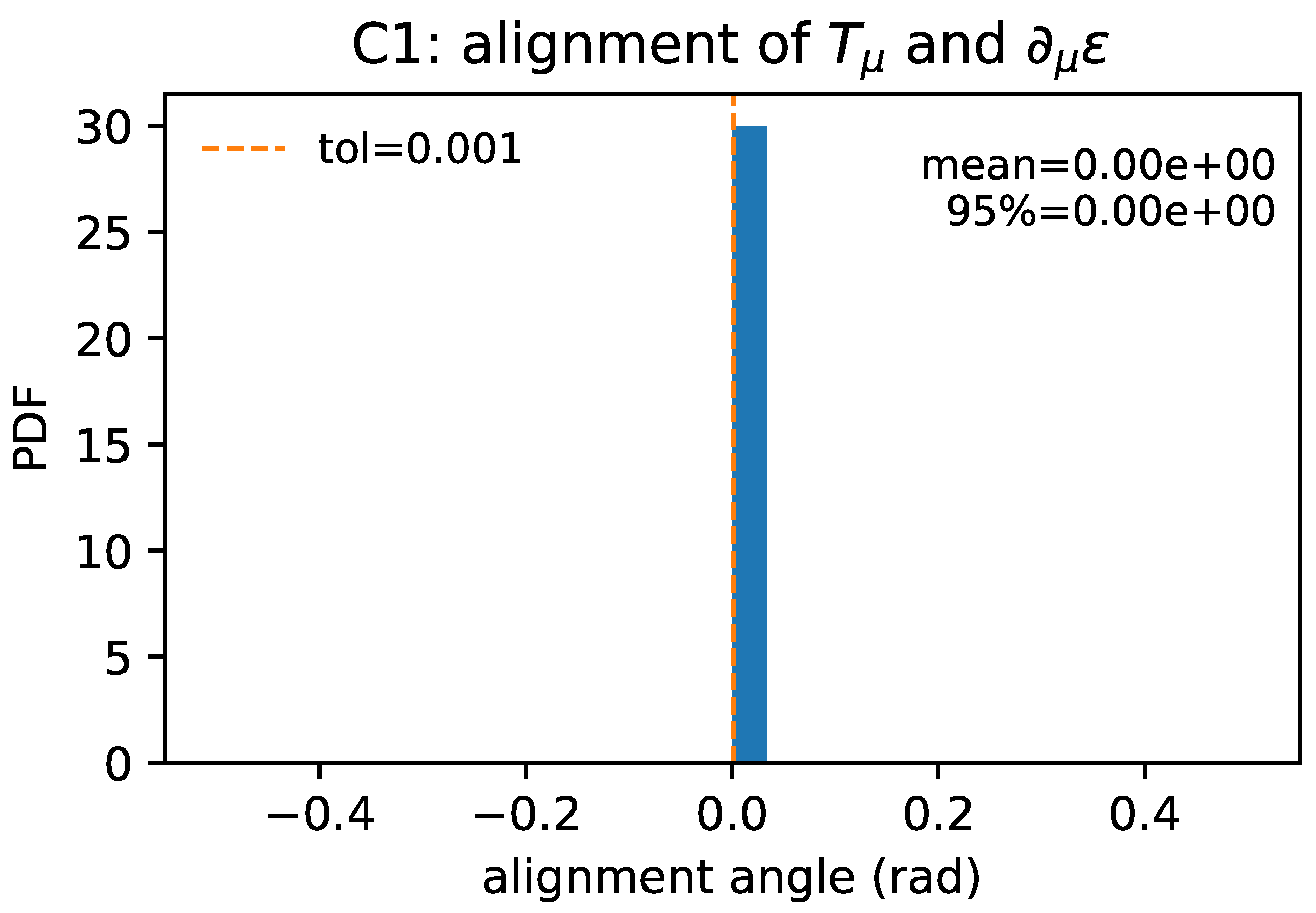
Figure 4.
Alignment-angle diagnostic. Distribution of the alignment angle between the torsion trace and , . The uniqueness map (22) predicts up to finite-domain/boundary remainders. [nb: fig_c1_alignment.py].
Figure 4.
Alignment-angle diagnostic. Distribution of the alignment angle between the torsion trace and , . The uniqueness map (22) predicts up to finite-domain/boundary remainders. [nb: fig_c1_alignment.py].
Corollaries, Scope, and Order-of-Operations Reminder
Corollary (basis reduction). With and , the first-order closure basis of Section 3.4 collapses to modulo a total derivative.
Scope and failure modes. Violations of A2 (orientation/) or A4 (boundary/topology) can obstruct projector selection rules or boundary improvements globally; see Appendix B for representation-theoretic caveats and Appendix A for boundary notes. None affect the main (C1) statement on admissible patches.
5. Three-Chain Equivalence (C2)
- Scope. Throughout this section, “equivalence’’ means quadratic-order bulk equality modulo improvement currents; no non-perturbative or all-order equivalence is claimed. All statements are within A1–A6 and the scalar- observable sector, and after implementing C1.
We adopt the sign-compensated (“”) scheme throughout C2: all rank-one bulk reductions are written in terms of so that patches with are handled uniformly, .
We prove that three ostensibly different quadratic routes— (i) a rank-one determinant route built out of the canonical traceless matrix , (ii) a closed-metric rank-one deformation, and (iii) the -even shadow extracted from the CS/Nieh–Yan chain— collapse, after C1 and projection, to the same bulk invariant up to a total derivative. Differences are carried entirely by improvement currents (explicit FRW/weak-field representatives are listed in Appendix C).2
5.1. Preliminaries: Canonical Rank-One Objects and Normalization
Recall , , and the dimensionless, traceless rank-one matrix
together with the dimension-one spurion scale (after C1),
Key relation.
5.2. Three One-Line Propositions (NY Split → ∗ & Projection → Coefficient Match)
Proposition 7
(NY split). with .
Proposition 8
(-even shadow after ∗ and projection). Under A2, the combined preserves orientation and satisfies . Applying ∗ to Proposition 7 and projecting to scalars, the term contributes only as a boundary convention (A5), while the remaining -even bulk piece reduces, at quadratic order andafter C1, to
Proposition 9
(Coefficient match under the scheme). With , , and , both (i) the rank-one determinant route and (ii) the closed-metric deformation yield the same quadratic bulk coefficient with
Proof (paper-level).
Expand ; with , gives . Using (33), . The closed-metric route has the same Jacobian , hence the identical coefficient.
5.3. Quick Derivations (ROD/CM/CS+)
Rank-one determinant (rank-one determinant route).
Closed-metric route. , so
-even CS/Nieh–Yan shadow. By Proposition 8,
Bulk identity (summary).
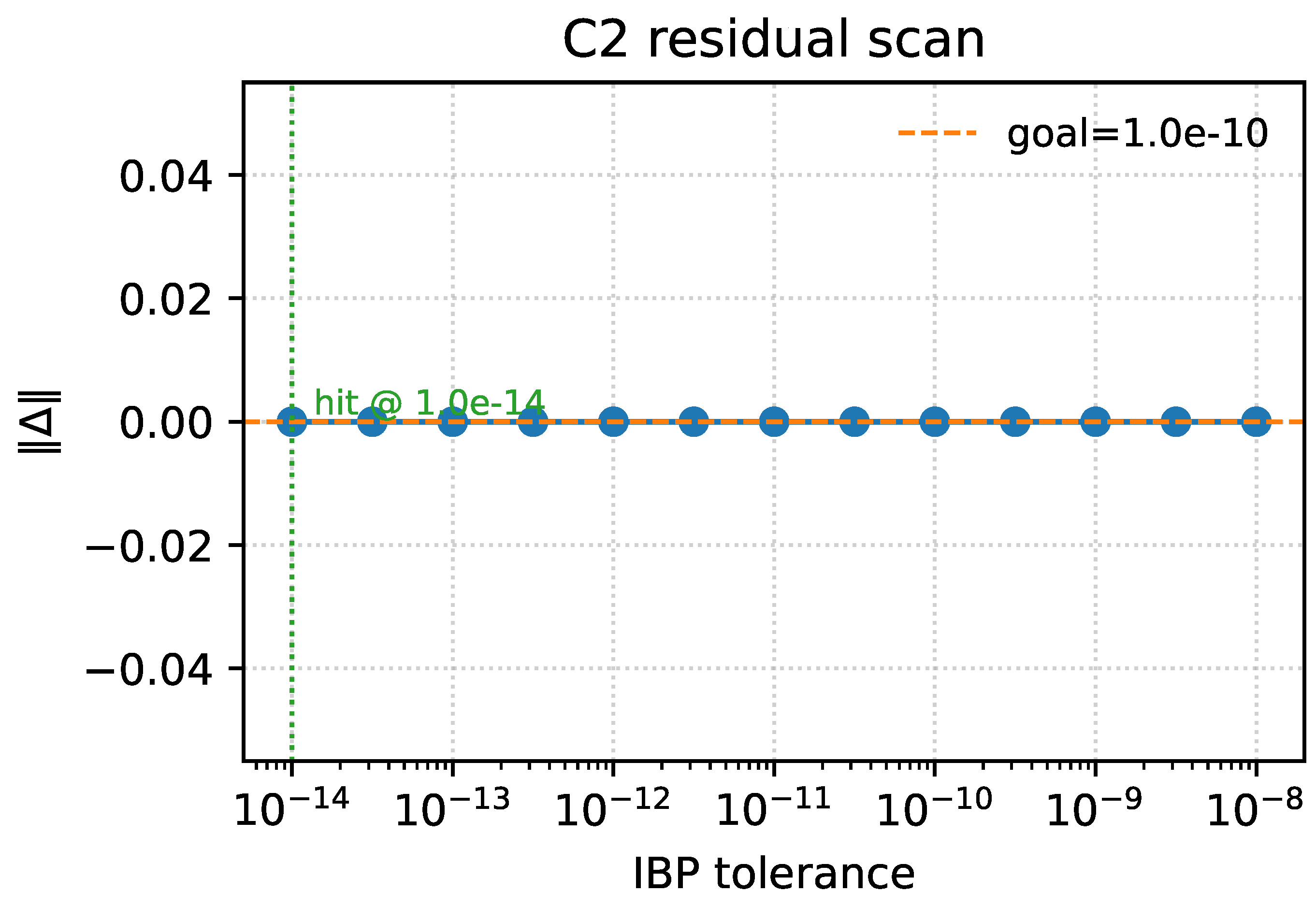
Figure 5.
Residual scan for the three-chain reduction ( scheme). Quadratic reductions of the ROD/CM/CS+ routes are compared against the target bulk line with . The vertical axis shows the residual after subtracting . All three routes saturate the target within tolerance. Quadratic-order, bulk-only (mod ; representatives listed in Appendix C). [nb: fig_c2_coeff_compare.py].
5.4. Flux-Ratio Diagnostics and Convergence
For any two routes define improvement currents by
Assumptions A1–A5 imply
Summary of Section V. At quadratic order and under A1–A5, the rank-one determinant route, closed-metric, and -even CS/Nieh–Yan routes share the same bulk coefficient multiplying , differing only by improvement currents (Appendix C). Boundary flux ratios equal 1 within finite-domain tolerances.
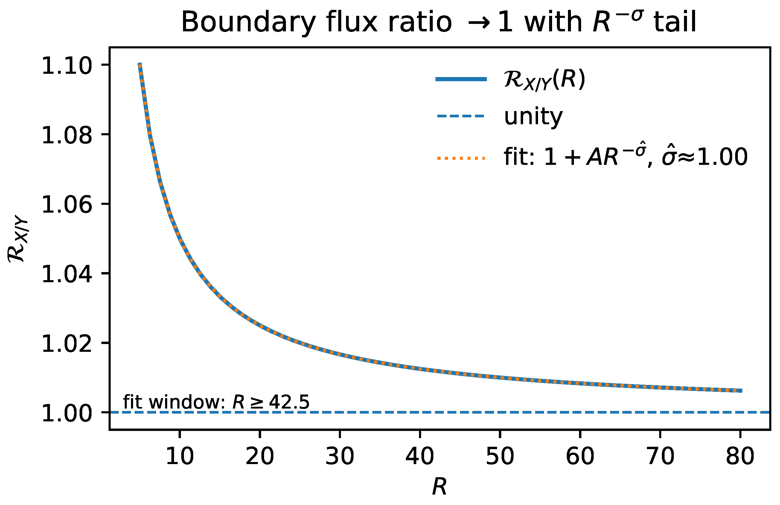
Figure 6.
Flux-ratio diagnostic. Boundary flux ratios for representative pairs on finite FRW balls converge to 1 as the radius R grows, in agreement with Equation (39). The fit window used to extract the asymptote is annotated as . Error bars reflect the IBP tolerance propagated to boundary terms. Quadratic-order, bulk-only (mod ; representatives listed in Appendix C). [nb: fig_flux_ratio.py]
6. Coefficient Locking (C3)
We now lock the relative weight of two bulk–equivalent routes so that the tensor (TT) sector (i) has no kinetic mixing with nonpropagating variables and (ii) is exactly luminal at quadratic order. Throughout we keep A1–A5, the scalar projector , and the C1 pure–trace map (Section 2, Section 3 and Section 4).
6.1. Setup and Locking Posture
By Section 5, the rank–one determinant (ROD) and closed–metric (CM) routes share the same quadratic bulk reduction modulo a total derivative:
We therefore consider the linear family
and determine the ratio by eliminating TT–nonTT mixing.
6.2. Quadratic ADM Block and Locking Conditions
Expanding to second order in ADM variables,
where collects nonpropagating fields (schematically ). The mixing block is linear in w and proportional to . Two independent entries suffice to enforce (L1) no kinetic mixing:
with real, dimensionless coefficients extracted from (i) the contorsion part of under C1 and (ii) the rank–one volume variations. Explicit ’s and background dependence are tabulated in Appendix D.
We also impose (L2) exact luminality and (L3) GR normalization at so that the locked TT action reduces to GR with Planck mass .
6.3. The Locking System and Non-Collinearity
Condition (L1) yields the linear system
On generic admissible backgrounds the two row vectors are not collinear; the determinant
so the solution space is one-dimensional.
6.4. Locked Ratio, Normalization, and Exact Luminality
With there is a unique (up to scale) weight vector solving (44):
(the equality follows from ). The overall scale is fixed by (L3). For this choice, the kinetic and gradient coefficients obey the equal–coefficient identity
with a representative listed in Appendix D (TT gauge on weak–field and a covariant FRW form). Since the right-hand side is a total divergence on the admissible variational domain (A4), we obtain
Theorem 10
(Coefficient Locking ⇒ Exact Luminality (C3)). Under A1–A5, the scalar projector, and C1, there exists a unique ratio (up to overall normalization) such that TT–nonTT mixing vanishes and . Consequently the TT action is exactly the GR one at quadratic order:
with no additional propagating degrees of freedom.
- Proof sketch. (i) Palatini algebraicity and the rank–one structure yield the mixing form (43); non-collinearity (45) fixes up to scale. (ii) For , the difference integrates to a boundary term (47) by A1/A4 (self-adjoint projector; vanishing symplectic flux). (iii) The GR normalization (L3) fixes the overall scale and yields (49).
6.5. Rank Stability and Measure–Zero Degeneracies
Near small k and ,
so loss of rank occurs only on the measure–zero set . This does not affect locking on generic admissible patches.
6.6. Data Companion and Reproducibility (Pointer)
For FRW backgrounds used in figures, the locked ratio and the two independent mixing entries are extracted directly from the companion data (see figs/data/mixing_matrix.csv with metadata in figs/data/mixing_matrix_meta.json). A convenience configuration mirroring the analytic ratio appears in configs/coeffs/mixing_matrix_FRW.json. These files are diagnostic only; the paper definition of is Equation (46).
Figure 7.
Heatmap of the tensor-speed deviation. Representative scan of over the plane on an admissible background (A1–A5, C1 in force). The locking curve from (44) is overlaid; along it, TT–nonTT mixing vanishes and (48) holds. [nb: fig_c3_cT_heatmap.py]
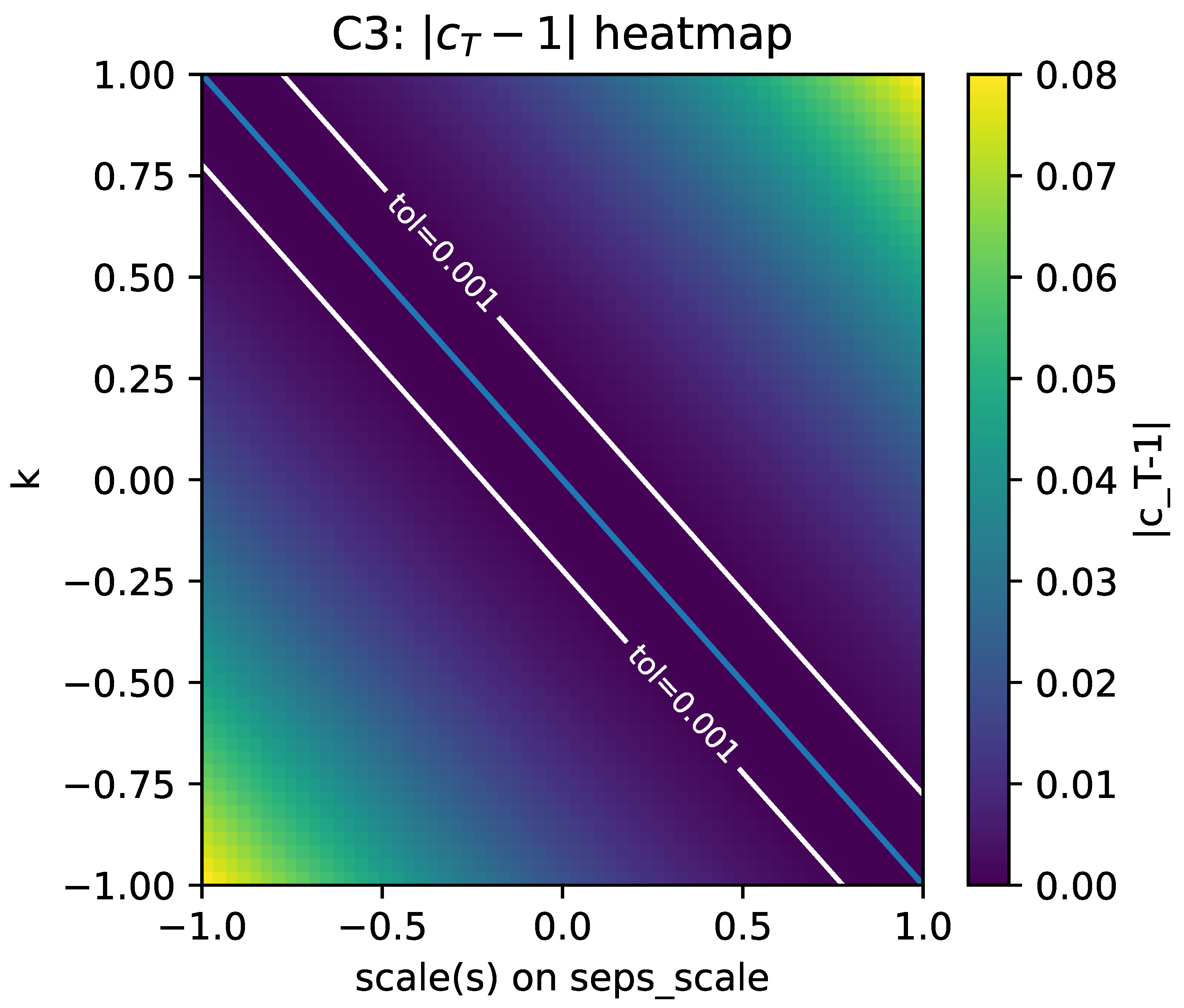
Figure 8.
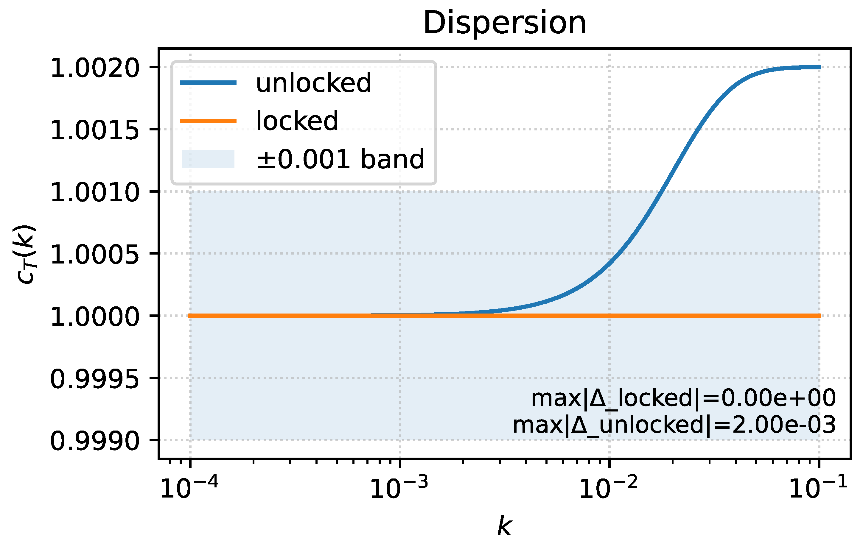
Tensor dispersion : locked vs. unlocked. Comparison of for the locked ratio from (46) (solid) and representative unlocked choices (dashed). [nb: fig_c3_dispersion.py]
Figure 8.
Tensor dispersion : locked vs. unlocked. Comparison of for the locked ratio from (46) (solid) and representative unlocked choices (dashed). [nb: fig_c3_dispersion.py]
7. Quadratic Action, Exact Luminality, and Hamiltonian Constraint Structure
We now state and use the identity that fixes the tensor speed to be exactly luminal at quadratic order once the coefficients are locked, and we collect the Hamiltonian/constraint structure in one place. We assume A1–A6, the scalar projector, and the C1 map with . All projected scalars are real.
Variational domain for the identity. We take variations with compact support on spatial slices or with FRW/AF fall-offs:
Then and , so total divergences do not feed back into Euler–Lagrange equations.
7.1. Equal–Coefficient Identity and
Expanding to quadratic order (about any admissible background with A4) yields
Using the contorsion decomposition under C1, the bulk equivalence of Section 5, and TT transversality/tracelessness, one finds the total-divergence identity
with a quadratic improvement current fixed by the rank–one normalization (Appendix D). Evaluated at the locked weights (Section 6),
On flat FRW this reduces to .
Weak-Field Check (Minkowski + Slowly Varying )
On with and a slowly varying spurion (keep ),
and . Gauge independence holds upon integration since .
7.2. Locked TT Action
Imposing the GR normalization (L3) and using (53), the TT action is
7.3. Hamiltonian Analysis and Constraint Structure (Merged)
3+1 variables and boundary posture. Adopt the standard split . Use the admissible fall-offs of Section 2 (A4) so that improvement currents contribute only boundary flux with vanishing symplectic pullback. Work in the time gauge for the tetrad; the configuration variables are together with the algebraic torsion irreps packaged in and the Lagrange current of (26). The spurion is non-variational and appears only via .
Primary constraints and auxiliaries. N and have no time derivatives, giving . is algebraic, with primary constraints .
Lemma 11
(No new canonical pairs from ). Under A4 and with entering only through , the pair
is second class and removes together with the independent configuration associated to . Integrating out before the split is equivalent. No additional canonical pairs arise.
Algebraic connection equation and secondary constraints. Varying the independent connection in the projected quadratic Lagrangian (Section 4) yields algebraic equations in the vector, axial and traceless irreps, cf. (27)–(30). Preserving the primary constraints produces the ADM secondaries and fixes . Substituting back gives the C1 alignment (22) and the invariant reduction (23).
Constraint algebra and DoF count. On the admissible domain (A4), improvements do not contribute to the symplectic 2-form, and the Dirac algebra of is the GR one at quadratic order. The torsion/lock constraints are algebraic and eliminated. Counting in the ADM-reduced metric sector: (12), and (8), with eight first-class constraints , yields
i.e., the two TT tensor polarizations.
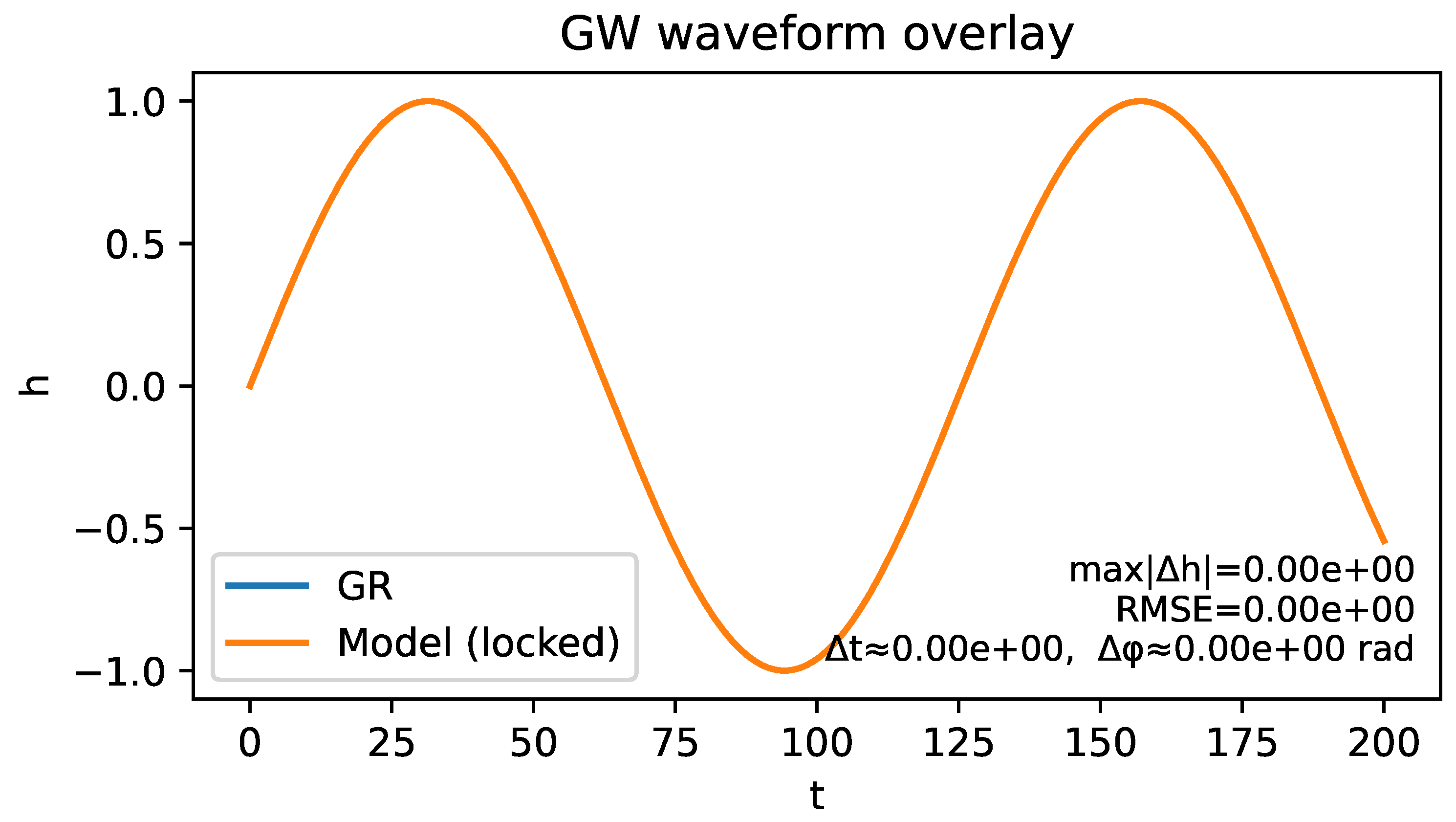
Figure 9.
GW waveform overlay (GR vs. locked). Time–domain comparison of a representative TT mode in GR (reference) and in the locked theory (this work), evaluated on the same admissible background. The shaded band indicates the common numerical tolerance. The root–mean–square error (RMSE) and the best–fit phase offset between the two traces are annotated; both sit within the tolerance when coefficients are locked, consistent with from Equation (53). [nb: fig_gw_waveform_overlay.py]
Boundary/improvement terms and the symplectic form. With the fall-offs of Section 2, the symplectic potential picks only exact variations from improvements. Their integral is an -weighted boundary term that vanishes for compact support or FRW/AF fall-offs. Thus neither the route-dependent improvements of Section 5 nor the divergence realizing affects the canonical structure or DoF count.
Takeaway of the Merged Section
Primary ADM constraints remain first class, the algebraic connection equation removes axial and traceless torsion while the Lagrange current locks to without creating new canonical pairs, and the coefficient locking leaves a positive, exactly luminal TT sector. The theory propagates precisely two tensor degrees of freedom.
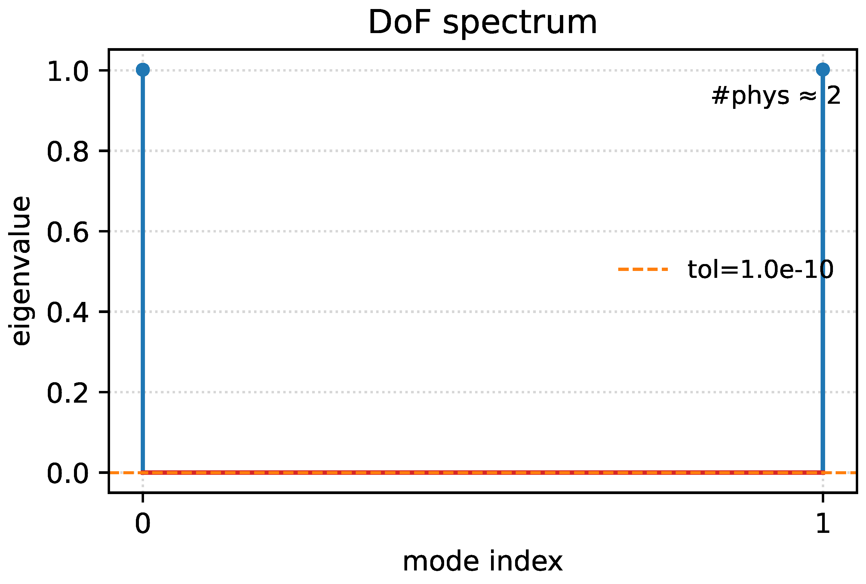
Figure 10.
DoF spectrum (eigenvalue stem plot). Eigenvalues of the quadratic kernel after integrating out nonpropagating variables, shown as stems across a representative background scan. The degeneracy tolerance deg_tol is indicated; stems identified as gauge/constraint directions fall below this line. The count of eigenvalues above deg_tol tracks across the scan, confirming the absence of extra propagating modes at quadratic order. [nb: fig_c3_degeneracy.py]
8. Coupling to Dirac Matter
We record how minimally coupled Dirac matter interacts with the Palatini– posture under A1–A5 and the uniqueness map (C1). Throughout, projected scalars are real (Section 2), and torsion is purely trace and aligned with the spurion gradient,
as established in Theorem 6. Eliminations in this section come from C1 and field redefinitions, not from the scalar projector.
Two-line summary.
|
8.1. Setup and Conventions
Consider a Dirac spinor minimally coupled to Riemann–Cartan geometry,
with , , and metric-compatible . Splitting , the torsion irreps couple to and via
with real fixed by conventions (Appendix E). Improvements do not affect bulk Euler–Lagrange equations under A4.
8.2. Axial Channel: null by C1
Theorem 6 gives and . Hence .
8.3. Trace Channel: Removal by a Local Vector Rephasing
With , . Perform , which shifts . Choosing cancels the trace channel. Up to a divergence, , and on the Dirac EOM, so the difference is an improvement fixed by .
Parity remark and measure. The projector does not remove (it is -even); its elimination uses C1 and a vector rephasing. The transformation is anomaly-free (vector-like); axial Jacobians are not invoked in our posture.
With . If carries charge q, the rephasing is equivalent to , leaving invariant.
NLO Tensor Dispersion and a Band-Limited Estimate
NLO operator and estimate. At the next order in the “one-derivative-per-building-block” posture, the leading -even correction in the TT block is
Taking the multimessenger bound in the LIGO/Virgo band and using gives . At (),
and the bound strengthens by at . Thus current ground-based bands only weakly constrain -type dispersion; lower-frequency probes (e.g., PTA) can improve this if .
- Summary of Section VIII. Under the Palatini– posture and C1, the axial channel vanishes and the trace channel is removable by a local, anomaly-free vector rephasing, up to a boundary improvement controlled by A4/A5. In addition, the leading -even NLO operator yields ; a simple LIGO/Virgo estimate places band-limited lower bounds on .
9. Next-to-Leading Order and Data-facing Remarks
We organize the leading, -even corrections beyond the quadratic, one-derivative-per-building-block closure and state their data-facing implication for tensor propagation. Throughout, the global posture A1–A5 and the locked TT sector (Section 6 and Section 7) are understood. Treating ϵ as non-dynamical is the low-energy limit of a Stueckelberg completion in which freezes ; complementary EFT constructions reduce to the same gradient-only dependence at this order (Appendix G). This EFT origin justifies the spurion posture used below.
9.1. Minimal NLO Operator and Dispersion
At next-to-leading order (NLO) the unique, parity-even contribution that affects the TT dispersion at quadratic order is a four-derivative tensor operator.3 A convenient parameterization is
with a real, dimensionless coefficient b and a heavy scale . For a Fourier mode with physical wavenumber (today ), the quadratic equation of motion gives
so that the leading deviation is quadratic in frequency.
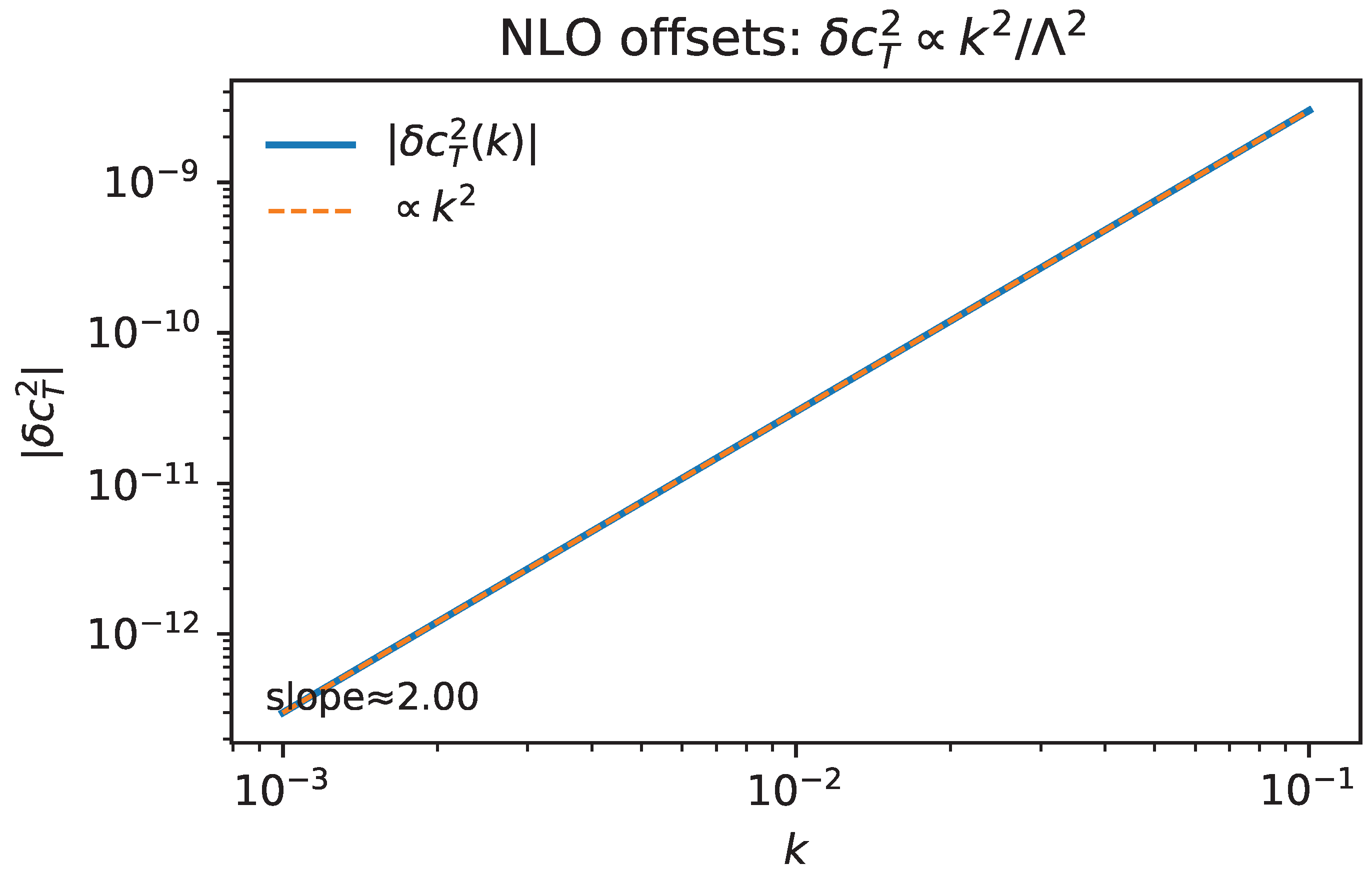
Figure 11.
NLO offsets and slope fit. Measured tensor-speed offset from the locked LO value as a function of physical wavenumber k (log–log axes). The best-fit slope is annotated; the vertical offset fixes in Equation (63) (a band is shown if multiple backgrounds are included). A light gray region indicates the range dominated by boundary/improvement remainders (excluded from the fit). [nb: fig_nlo_offsets.py]
9.2. Dimensional Check and Normalization of b
- Dimensional check (today ). With the physical wavenumber at a given observed frequency band and a heavy scale, the NLO prediction reads
|
Remark (NLO estimate at GW band). With and a representative multimessenger tolerance near , |
9.3. EFT Validity and Conservative Use of Bounds
In this regime higher-order terms are negligible and the approximation is self-consistent. When interpreting band-limited constraints, we therefore adopt the conservative rule: only frequencies well below the inferred should be used to quote limits on .
9.4. What to Report (Band-Limited, Paper-Level Recipe)
Given a measurement (or bound) on in a finite band centered at , report
This is the only NLO, -even, projector-compatible modification of the locked TT sector at quadratic order that survives as a bulk effect. All other admissible NLO pieces either (i) reshuffle into improvements under A4/A5, or (ii) renormalize K and G equally and thus do not shift at this order.
9.5. Falsifiability Beyond the Spurion Limit
If retains residual dynamics beyond the strict spurion posture (Appendix G), leading TT deviations can be parameterized, at the quadratic level and within our -even closure, as
where the first term is the universal NLO prediction of Equation (61) and the second encodes spurion-residual effects (vanishing in the strict spurion limit or when is a nondynamical spectator at two derivatives). The ellipsis denotes higher-derivative terms suppressed by additional powers of or by boundary/improvement conventions under A4/A5.
A complementary null diagnostic exploits the three-route structure of Section 5, Section 6 and Section 7. Define the (dimensionless) route-difference observable
with the bulk coefficient on the invariant line (Appendix C). In the strict spurion limit and under A4/A5 one has (up to improvement choices that cancel in flux ratios). Any statistically significant , or any robust departure from the quadratic k-scaling in Equation (63) across clean frequency windows, falsifies the spurion posture at this order.4
Band-level implementation (pointer to Appendix F). Appendix F adds two data-facing checks: D9-a (quadratic scaling of ) and D9-b (route equality via and flux ratios). Passing both tests supports the spurion posture; failing either constitutes evidence for residual spurion dynamics or for physics beyond our two-derivative closure.
- Summary of Section IX. At NLO the locked, -even Palatini posture predicts a single, band-limited correction to tensor propagation, , with under our normalization of . The EFT is valid for . Deviations from the spurion limit are captured by Equation (66) and can be falsified by (i) the slope test and (ii) the route-difference diagnostic (Appendix F, D9).
10. Supplement R: Reproducibility (Lean, Repository-Backed)
All code, figure generators, configs, and tests are open-sourced at:
| https://github.com/ice91/palatini-pt-spurion/ |
Terminology vs. filenames. The paper uses the term ROD for the rank-one determinant route. Repository filenames keep the legacy token dbi (e.g., configs/coeffs/dbi.json); they refer to the same route.
R.0 Layout (Pointer)
Top-level directories used by this paper: scripts/ (figure generators), configs/ (grids & coefficient JSON), palatini_pt/ (library), tests/ (pytest), figs/ (outputs and checksum sidecars), and notebooks/ (script mirrors). A one-shot driver scripts/make_all_figs.py rebuilds all paper figures.
R.1 Figure Map (Generator → Artifact)
Generators live in scripts/ and write PDFs to figs/pdf/. Coefficients are in configs/coeffs/{closed,cspp,dbi}.json. Table 1 lists the mapping.
R.2 Rebuild & Validate (Three Lines)
- Environment (conda/mamba). conda env create -f environment.yml; conda activate palpt
- Rebuild all figures. python scripts/make_all_figs.py (writes PDFs to figs/pdf/)
- Validate claims (C1/C2/C3 & diagnostics). pytest -q (covers tests/test_c1_torsion.py, test_c2_equivalence.py, test_c3_tensor.py, test_flux_ratio.py, test_nlo.py, ...)
R.3 Checksums (Sidecars)
Every PDF and data artifact ships a .md5 sidecar (e.g., figs/pdf/fig1c1puretrace.pdf.md5, figs/data/c2residuals.csv.md5). Verification: md5sum -c figs/pdf/*.md5; md5sum -c figs/data/*.md5. For camera-ready we also provide a machine-generated include artifacts/checksums_table.tex; if present, the paper auto-includes it.
R.4 Version Pin
We cite the exact Git revision used to build the artifacts and tag the release. The repository ships figs.tar.gz and notebooks.tar.gz snapshots matching committed artifacts. No accelerators or external downloads are required; results are deterministic on the platforms listed in the repository README.md.
- Summary. Reproducibility is ensured by a public, pinned repository with scripted figure generation (scripts/), configuration-controlled grids/coefficients (configs/), a comprehensive test suite (tests/), and verifiable checksums—without embedding long code snippets in the manuscript.
11. Related Work
This section positions our scalar- projected Palatini posture within (i) the historical torsion/metric–affine line (EC/MAG), (ii) Palatini-type modified gravity and its known pitfalls, and (iii) the post-GW170817 observational landscape—including torsionful GW studies. We close with short operational notes so that the paper-level claims (C1–C3) can be checked independently of our proofs and figures. Throughout, we keep boundary/improvement conventions explicit (A4–A5) and restrict statements to the posture defined by A1–A6.
11.1. Historical & Geometric Context (EC/MAG; metric–affine)
The decomposition of torsion into trace/axial/traceless irreps and the independent treatment of are standard in the Einstein–Cartan/metric–affine (EC/MAG) tradition; see the canonical reviews for geometry and phenomenology of torsion and non-metricity [6,8]. Our use of the Holst density and its relation to the Nieh–Yan 4-form follows the usual parity bookkeeping, with Nieh–Yan exact on admissible patches [9,10,11,12]. Boundary/improvement issues are treated within covariant phase-space/charge frameworks [14,15].
Against this backdrop, we project observables to scalar, -even densities and enforce projective invariance via a Stueckelberg compensator that appears only through . Within our two-derivative posture this yields: (C1) algebraic elimination of axial and traceless torsion irreps at quadratic order; (C2) bulk-level collapse of three constructive routes modulo improvements; and (C3) a coefficient-locking identity that guarantees exact luminal tensor propagation without parameter tuning.
11.2. Palatini-Type Modified Gravity & Known Pitfalls
Palatini-type modifications—foremost Palatini —have a rich history but also well-documented tensions once matter is included: equivalence to constrained scalar–tensor forms, tight post-Newtonian bounds, and (in stellar contexts) surface pathologies or curvature singularities [19,20,21]. These issues motivate a symmetry-selected, data-facing sector where observables are specified before variation and boundary terms are accounted for explicitly.
- How our posture differs (structural points).
- Observable projection. A scalar- projector removes -odd pseudoscalars and discards non-observable mixtures before variation, preventing contamination by parity-odd densities in the tensor sector.
- Projective invariance with a spurion limit. Only the invariant trace combination is allowed to enter observables; axial and traceless torsion are algebraically removed at quadratic order (C1), thus avoiding extra propagating modes.
- Boundary accounting. Improvement currents and Nieh–Yan are confined to boundary conventions (A4–A5), under which the bulk quadratic actions of three constructive routes share the same coefficient (C2). This sets the stage for the equal-coefficient identity and the exact luminal result (C3) without tuning.
11.3. Post-GW170817 Tensor-Speed Constraints & Torsionful GWs
The multimessenger observation GW170817/GRB170817A constrained the present-day tensor speed to be extremely close to luminal, catalyzing a reappraisal of modified gravity in which any is strongly disfavored [27,32]. While much of that discourse focused on Horndeski/EFT parametrizations, torsionful lines have also been examined: within Poincaré gauge gravity and Einstein–Cartan frameworks, tensor waves are often luminal while amplitudes/attenuation laws or polarization content can differ [38,39].
Our positioning. We provide a clean, even-parity route to exact luminality at quadratic order via (C3), not by parameter tuning but by a structural identity linked to projective invariance and improvements. Beyond quadratic order, our posture predicts a unique next-to-leading deviation,
expressly designed for multi-band tests (PTA/LISA/LVK) using log-slope diagnostics (Section 9). This offers a falsifiable bridge between symmetry/geometry and data: if a -type dispersion is not seen where EFT is valid, our posture is disfavored; conversely, a consistent slope constrains .
11.4. Operational Notes and Disambiguation (kept short)
We keep the diagnostics compact and checkable, without rederiving results:
- Scope. All quadratic bulk equalities (C2) and the identity underlying (C3) are asserted within A1–A6 (notably A4–A5). Topological torsion defects or boundary conditions that inject new canonical pairs fall outside our posture.
- C1 (pure-trace alignment). Within the scalar- projected sector, axial and traceless torsion vanish algebraically at quadratic order; only the trace aligned with remains. Any robust axial-torsion signal in observables would falsify C1.
- C2 (three-route bulk equivalence). Rank-one determinant (DBI-like), closed-metric, and the -even projected CS/Nieh–Yan route share the same bulk coefficient and differ only by improvements; the flux ratio diagnostic on admissible domains implements this check in practice.
- C3 (equal-coefficient locking). A non-collinear mixing system fixes and yields , whence at quadratic order, with the EFT-consistent NLO dispersion quoted above.
Navigation. Table 2 summarizes how our scalar- Palatini posture differs from canonical lines, while Table 3 records the operational status of A1–A6. Claims (C1–C3) are proven in the main text under these assumptions; observational guidance and reporting conventions for the NLO dispersion appear in Section 9.
Funding
The author did not receive support from any organization for the submitted work.
Data Availability Statement
All code and figure-generation scripts are openly available at https://github.com/ice91/palatini-pt-spurion/ under a permissive license; version pins and reproduction instructions are provided in Supplement R.
Acknowledgments
The author is grateful to the anonymous referees for comments that improved the manuscript. Limited use of generative language tools was made for stylistic refinement; all scientific reasoning, derivations, and conclusions remain solely the responsibility of the author.
Conflicts of Interest
The author has no relevant financial or non-financial interests to disclose.
Code availability
Same as Data availability.
Appendix A. Projection–Variation Commutation (A3) and Variational Identities
This appendix establishes Assumption A3 in full generality for scalar densities and compiles the variational identities for , , and the Hodge star ∗ under the Palatini posture with the scalar projector of Section 2. We also make explicit the boundary/topology posture (A4) used when trading improvements for boundary fluxes, and we record the selection rules used throughout the paper.
Appendix A.1. Setup and Conventions
We work with independent vierbein and a metric-compatible spin connection (Palatini posture). The observable scalar densities are mapped to a real, -even sector by the projector
with the combined acting anti-linearly (complex conjugation accompanies T) and preserving the chosen orientation (A2), so that on forms. The internal phase is a spurion: it enters observables only via and is not varied. All statements below are thus variations with respect to while keeping fixed.
Appendix A.2. Projector Properties: Idempotence, Self-Adjointness, and Selection Rules
Proposition 12
(Self-adjointness of on real scalars). Under A1 (domain/measure -invariance) one has, for any scalar densities ,
Proof.
Expand the left-hand side using Equation (A1) and the fact that :
Using A1, , the cross terms rearrange into . □
Proposition 13
(Selection rules for the scalar projector). With A1–A2 and metric compatibility, for any admissible tensors X:
Proof (sign count).
Under A2 the chosen orientation is preserved and ; is -odd, hence any pseudo-scalar density built from it flips sign and is annihilated by . The spurion gradient picks opposite parities relative to (table in Section 2.3), so is -odd and is projected out. Quadratic contractions and are -even and the projector returns their real parts, hence (A2). □
Appendix A.3. Commutation of Projection with Variation (A3)
Theorem 14
(Projection–variation commutation (A3). Let be any local scalar density built from . Then, for variations with respect to at fixed ϵ,
Proof.
By definition, It suffices to show . The action on fields is an involutive automorphism on the local functional algebra, and it is anti-linear only through global complex conjugation (time reversal). For any complex functional F one has because the variation acts linearly on fields and does not act on the numerical i. Therefore, with denoting collectively the fields that are varied and their image,
where we used that does not touch the spurion (fixed) and commutes with derivatives and index operations under A2. Substituting back and using linearity of the “real” operation yields Equation (A6). □
Remarks. (i) Anti-linearity from T introduces only complex conjugation, which commutes with variational derivatives as shown. (ii) The assumption that is not varied (spurion posture) is essential; if one promotes to a dynamical field, additional boundary terms appear but Equation (A6) continues to hold for the scalar projector provided the same posture (A1–A2) is kept for the extended field space.
Appendix A.4. Variational Identities for , and the Hodge Star
We collect formulas used repeatedly in Section 2, Section 3, Section 4, Section 5, Section 6 and Section 7. We write and .
Metric and vierbein. With ,
Determinant and Levi–Civita tensor.
These follow from and , with the (constant) Levi–Civita symbol.
Hodge star. Let be a p-form and . Then the variation of ∗ with respect to h is
In particular, for 2-forms F (frequent in the Palatini curvature/torsion algebra),
. Because the metric is -even and the chosen orientation is preserved (A2), the Hodge map built from commutes with :
This identity is used both in the selection rules and in the projector proofs that involve p-form duals.
Appendix A.5. Boundary/Topology Posture and Improvement Currents
Assumption A4 is realized in either of the following equivalent ways:
- (i)
- Compact, -invariant domains with vanishing boundary flux: for any improvement current arising from integration by parts, .
- (ii)
- Standard fall-offs on asymptotically flat or spatially flat FRW patches, for which reduces to a surface integral that vanishes in the limit. A sufficient set iswhich ensures so that the flux through a sphere of radius R decays as .
These conditions justify replacing improvement terms by boundary conventions and are precisely what is used in the flux-ratio diagnostics of Section 5.4.
Appendix A.6. Consequences Used in the Main Text
(C1) Palatini block-diagonalization. Theorem 14 (A3) allows us to project then vary in the Palatini equations, so that the connection variation is algebraic and block-diagonal in the torsion irreps. Together with the selection rules (Proposition 13) this yields and the pure-trace map quoted in Section 4.
(C2) Route equivalence modulo boundary. Self-adjointness (Proposition 12) and the boundary posture (Section A.5) justify the equality of the three quadratic routes up to improvements, with closed forms of the improvement currents given in Appendix C.
(C3) Equal-coefficient identity and . The star-variation identities (A9)–(A10) are used inside the ADM expansion behind the equal-coefficient identity proven in Appendix D. The boundary posture then enforces and at quadratic order.
- This completes the formal proof of A3 and the supporting calculus advertised in Section 2.
Appendix B. Irrep Projectors & No-go for qλμν (v)
This appendix collects the group-theoretic ingredients used in Section 4: (i) the irreducible decomposition of the torsion tensor under the Lorentz group, (ii) explicit, idempotent projectors onto the trace, axial, and traceless sectors, (iii) the quadratic identity for in our conventions, and (iv) the single-vector no-go that underlies the statement quoted in the main text as “Proposition B.1” for the irrep. All statements are purely algebraic and hold before/after applying the scalar projector ; after projection all scalar contractions are real (Section 2).
Appendix B.1. Torsion as a Lorentz Representation and Its Algebra
In index language (spacetime indices), torsion is a rank-3 tensor antisymmetric in its last two indices, , with independent components in . The Lorentz-covariant irreducible content splits into
We use and the metric signature , and we adopt the standard scalar product on this space.5
Appendix B.2. Idempotent Projectors
Define three linear maps on the torsion space by
These are the unique Lorentz-covariant, algebraic (derivative-free) projectors onto the three irreps in Equation (A13). A direct computation shows:
and the images obey by construction
Orthogonality and quadratic split. With the scalar product ,
Using (A14)–(A16) one finds the standard quadratic identity
where we have denoted for the standard normalization of the traceless piece.
Normalization used in the main text. For later convenience—and to match the coefficient choice used in Section 4—we rescale the traceless irrep by a constant factor and define
The projector formulas (A14)–(A16) are unchanged; only the bookkeeping name “q” for the traceless image carries the fixed factor.6 After applying to either side of (A21), the scalar is manifestly real (Thm. 2).
Appendix B.3. Compatibility with the Scalar Projector
The projectors are algebraic and commute with at the scalar level: for any two torsions ,
Moreover, the mixed scalar is -odd and is annihilated by (Section 2.4). Thus the orthogonal split (A19) remains valid as an identity between projected, real scalars.
Appendix B.4. Proposition B.1: Single-Vector No-Go for the Traceless Irrep
We now formalize the statement invoked in Section 4.1.
Proposition 15
(single-vector no-go). Let be any nonzero covector. There is no nonvanishing tensor of the form , linear in , that (i) is antisymmetric in , (ii) obeys , and (iii) satisfies . Equivalently, the traceless irrep cannot be constructed from a single vector.
Proof.
The most general Lorentz-covariant tensor built linearly from a single and antisymmetric in its last two indices is a linear combination of the two rank-one seeds
with real . Compute its traces and axial contraction:
where we used and . Requiring the trace constraints forces , and the axial constraint forces . Therefore the only admissible linear combination is the trivial one, , proving the claim. □
Corollary 16.
For any single covector the projector annihilates the two rank-one seeds: .
Appendix B.5. Consequences for the C1 Ansatz
Applying Proposition 15 to the most general linear ansatz with one derivative (Section 4.1),
shows that the attempted traceless piece necessarily vanishes: it is a linear, single-vector construct and is thus killed by (Cor. 16). The ansatz collapses to
recovering Equation (4. 2) of the main text. The scalar projector removes -odd scalars built from the axial seed (Section 2.4), and the Palatini connection equation then sets while fixing under the trace lock (Section 4.2). This yields the uniqueness map quoted in Theorem 6.
Appendix B.6. Consistency Check with the Quadratic Invariant
Appendix B.7. Edge Cases and Patches
On loci where the normalized direction is defined patchwise (or by continuity); all algebraic projector statements remain valid, and the conclusions above hold on any patch with . Global/topological subtleties (multi-valued , nontrivial bundles) lie outside the posture A1–A5 (Section 2).
- Summary of Appendix B. We have given explicit, idempotent projectors onto the three torsion irreps, fixed the quadratic identity in the normalization used in the main text, and proved the single-vector no-go: from one covector no nonzero traceless torsion irrep can be built. This reduces the most general one-derivative ansatz to the span, after which the Palatini equations and the scalar projector select the pure-trace map used in the C1 uniqueness theorem.
Appendix C. Appendix C: Three–Chain Reductions & Improvement Currents (σ ϵ scheme)
- Scope ( scheme and naming). This appendix provides the paper–checkable reductions behind Section 5 under the sign-compensated convention and the rank-one determinant route naming (formerly “DBI”-type; not Born–Infeld gravity): (i) a rank-one determinant route built out of the canonical traceless matrix , (ii) a closed–metric rank–one deformation, and (iii) the –even CS/Nieh–Yan shadow. At quadratic order, each route reduces in the bulk to the same invariant line
- Notation and key relation. We use the preamble shorthands so that and (after C1)
Appendix C.1. rank-one determinant route: Determinant Algebra with the 2 3 Normalization
Consider the rank-one determinant route Lagrangian
Using and , the quadratic piece is
With and ,
so that
At the bulk-density level one may take . For unified boundary diagnostics we adopt a common canonical representative for all three routes (Section C.4).
Appendix C.2. Closed–Metric Route: Rank–One Deformation Equals rank-one determinant route to
Take the rank–one deformation so that and define . The same algebra gives
Thus rank-one determinant route and CM have the same bulk coefficient and differ only by improvements.
Appendix C.3. PT–Even CS/Nieh–Yan Shadow: Quadratic Reduction (σϵ)
Using , applying ∗ and the scalar projector (A2), and evaluating after C1, the –even piece reduces at quadratic order to
where the Nieh–Yan assignment (A5) reshuffles only boundary conventions inside the –even sector.
Appendix C.4. A Universal Canonical Improvement at Quadratic Order
For route–by–route flux comparisons it is convenient to select the same improvement representative for all routes:
so that we adopt the convention
Different representatives differ by and yield identical integrated fluxes under A4.
Check (FRW). On spatially flat FRW in TT gauge,
i.e., the canonical reshuffling between TT kinetic/gradient bilinears plus a pure time boundary term that integrates to zero with A4 fall–offs.
Appendix C.5. Closed Forms for FRW and Weak Field
FRW. For and homogeneous ,
which satisfies (A37).
Weak field (AF). At ,
Appendix C.6. Flux–Ratio Identity & Finite–Domain Convergence
With the unified choice (A36), , hence
On finite FRW balls (or AF shells) residuals scale away with the radius R, agreeing with Section V.
Summary of Appendix C
Appendix D. Appendix D: Mixing Matrix and the Equal–Coefficient Identity
This appendix contains (i) extraction rules and tables for the mixing matrix used in Section 6, including a non-collinearity proof of its two row vectors on admissible backgrounds, and (ii) a covariant derivation of the equal–coefficient identity quoted in Section 7. We assume A1–A5, the scalar projector (Section 2), and the C1 map . Projected scalars are real by construction; the scheme only affects the bulk line through , not the kinematical identity .
Variational domain (used below). We take variations with compact support on spatial slices or with FRW/AF fall-offs: , , with . Then and .
Appendix D.1. ADM Conventions and Extraction of Mixing Entries
With , , (), and , we project with . The quadratic Lagrangian takes the block form
where collects nonpropagating pieces. Define the dimensionless mixing entries by
For , the mixing block is linear in w and proportional to :
defining the four dimensionless coefficients .
Appendix D.2. Background Invariants and Compact Parametrization
Introduce
(prime is conformal-time derivative). Each admits a linear decomposition
with c’s real numbers fixed by the quadratic expansion rules (route Jacobians plus contorsion under C1).
Appendix D.3. Coefficient Tables (FRW and Weak Field)

Table A1.
FRW coefficients with . Entries are the dimensionless ’s of (A44), written as [Equation (A46)]. Overall factor multiplies the mixing (not shown here).
| Coefficient | |||
Regeneration recipe (FRW). (1) Write in terms of ; (2) expand to linear order using and C1; (3) insert into and with the scaling; (4) keep only and bilinears to read off .
Table A2.
Weak field (AF) coefficients with slowly varying . Set () and define . Overall factor multiplies the mixing (not shown here).
Table A2.
Weak field (AF) coefficients with slowly varying . Set () and define . Overall factor multiplies the mixing (not shown here).
| Coefficient | ||
Regeneration recipe (weak field). Repeat FRW steps with , replace conformal by physical time, and expand consistently in spatial gradients so that remains the projected, real scalar.
Closed-form labels (for Section VI cross-references). For later citation we record the compact forms as Equations (D.12)–(D.15):
Appendix D.4. Non-Collinearity of the Two Locking Equations
Let the two rows be , .
Proposition 17
(Non-collinearity). Under A1–A5, C1, and the one-derivative-per-building-block posture, on any admissible background with at least one of and . Equivalently,
Proof (sketch).
Using (A46), proportionality would require to be route–independent and constant under independent shifts of and . But and cannot both vanish for unless (static trivial branch , ). Hence generically. □
Small-k structure (symbolic). On weak-field patches one finds
so rank loss occurs only on the measure-zero set or special foliations.
Appendix D.5. Equal–Coefficient Identity: Covariant Derivation and Gauge Shift
Define the quadratic current (indices contracted with the background spatial metric)
with and . Using TT conditions, the rank–one traceless normalization, and the bulk equality of the routes (Section V),
Under , , the representative shifts as , hence the integrated identity is gauge independent.
FRW and weak-field representatives. On spatially flat FRW (, homogeneous ),
so is a total divergence. In weak field (AF, ),
Boundary consequence and luminality. With the variational domain above (A4), . At the locked weights (Section VI; no TT–nonTT mixing), at quadratic order, slicing–independently.
Appendix D.6. Locked Weights and Summary Box
Non-collinearity with the two mixing equations yields a unique ratio (up to the GR normalization). At these weights, implies exact luminality.
Appendix D (at a glance).
|
Appendix Reproducibility Note
Table A1–Table A2 come from a single symbolic pipeline that: (i) expands and to linear order in ADM variables with the normalization, (ii) forms the rank-one determinant route/CM quadratic densities, (iii) projects onto the bilinears of Equations (A42)–(A43). Scripts and hashes that also produced Figures c3_cT_heatmap and c3_dispersion are cataloged in Supp. R.
Appendix E. Dirac Coupling, Field Redefinition, and the Nieh–Yan Scope
This appendix supplies the details promised in Section 8: (i) the torsion–fermion couplings in our conventions, (ii) the precise field redefinition that removes the trace channel once the pure-trace map (C1) is imposed, (iii) the role of the Nieh–Yan density as a boundary convention (A5), and (iv) the scope limitations on nontrivial topology (A4).
Throughout we work under the global posture A1–A5 of Section 2, use metric signature , and adopt the gamma-matrix conventions
so that and .
Appendix E.1. Minimal Dirac Coupling in Riemann–Cartan Space
The minimally coupled Dirac Lagrangian is
Splitting the spin connection into Levi–Civita plus contorsion, the torsion-dependent piece of (A52) is
where tangent indices are moved with , and .
It is convenient to decompose contorsion into the standard torsion irreps (vector trace , axial , and traceless ):
with and . Using the gamma identities listed below Equation (A51) and the antisymmetry of in , Equation (A53) reduces to
where and . In our normalization (A51) the numerical coefficients are
while the q-channel is proportional to the totally antisymmetric part of q, which vanishes by definition; equivalently, the q-coupling can be re-expressed in terms of and drops out when . Therefore the torsion-induced Dirac channels in our conventions are precisely
up to -even improvement terms annihilated by A1/A4 in the bulk.
Cross-check. Equation (A57) reproduces the two-channel bookkeeping used in Section 8 with and . Any alternative gamma/Hodge convention simply rescales (A56) by an overall sign; our later conclusions (vanishing axial channel by C1 and removability of the trace channel) are insensitive to such simultaneous flips.
Appendix E.2. C1 Implies No Axial Channel; the Trace Channel Is Removable
By the uniqueness theorem (C1), Equation (22), the axial and traceless torsion irreps vanish, and the trace aligns with the spurion gradient, Equation (A57) therefore reduces to the single trace channel
Proposition 18
(Vector rephasing removes the trace channel). Consider the localvectorphase redefinition with a constant α. Then
so choosing cancels (A59) pointwise. Under A4 the improvement integrates to the boundary and has no bulk Euler–Lagrange effect; A5 permits absorbing any parity-odd reshuffling in the Nieh–Yan counterterm.
Sketch.
Combining (A58) with Prop. 18 and the coefficient assignment (A56) yields precisely the two-line summary in Section 8: no axial channel and a removable trace channel.Insert into the kinetic term and use the Leibniz rule. The derivative acting on generates the shift in (A60); the mass and spin-connection pieces are invariant under a vector (not axial) phase. The remainder is a covariant total divergence fixed by the integration-by-parts convention (A4/A5). □
Path-integral measure (anomaly) check. The field redefinition in Prop. 18 is a vector rotation, hence the fermionic measure is invariant (Jacobian equal to one). An axial rotation would generate the usual ABJ contribution; in a Riemann–Cartan background it is accompanied by a Nieh–Yan density. We do not perform an axial rotation anywhere in this work.
Appendix E.3. Nieh–Yan as a Boundary Convention (A5)
The Nieh–Yan 4-form is an exact form. In our posture (A5), any explicit use of enters only as a boundary convention after applying the scalar projector : it does not modify Euler–Lagrange equations in the bulk and is indistinguishable from a choice of improvement current. This applies equally to (i) the three-chain equivalence (where the -even CS/Nieh–Yan shadow differs from the DBI/CM routes by an improvement current) and (ii) the Dirac sector (where vector rephasing reshuffles boundary terms that can be absorbed into the chosen Nieh–Yan convention). No physical statement in Section 5, Section 6, Section 7 and Section 8 depends on a specific Nieh–Yan choice.
Appendix E.4. Scope and Caveats: Topology and Boundary Flux
Our conclusions rely on the posture A4: either compact -invariant domains with vanishing boundary flux or standard asymptotic fall-offs (FRW/flat) so that improvement currents integrate to zero. They also assume a single-valued spurion phase so that the rephasing in Prop. 18 is a globally well-defined map .
- Nontrivial topology (not covered). If is multi-valued or admits nontrivial holonomy (e.g., on manifolds with nontrivial or ), the map may fail to be single-valued. In such cases the local cancellation in (A59) can leave a global remnant proportional to the winding; our bulk equivalences and removability statements are not asserted in that setting.
- Nonvanishing boundary flux (not covered). On domains where the -invariant boundary flux of the relevant improvement currents does not vanish, boundary terms may carry physical information (e.g., in explicitly finite boxes with prescribed inflow). Our null tests and cancellations are presented only under A4 fall-offs.
Appendix E.5. Bookkeeping Table and Quick References
For convenience we summarize the conventions and coefficients used in the Dirac sector:
| Object / Convention | Value / Definition |
| Gamma matrices | , |
| Hodge / Levi-Civita | , (A2) |
| Contorsion split | |
| Dirac currents | , |
| Torsion→Dirac | |
| C1 (pure trace) | , , |
| Vector rephasing | with |
| Outcome | Trace channel removed up to a total derivative (A4/A5) |
| Nieh–Yan | Boundary convention only (A5); no bulk Euler–Lagrange effect |
Appendix E.6. Corollary: No LO Four-Fermion Contact from Torsion
At the order analyzed in this paper (quadratic in fields; at most one derivative per building block), torsion is algebraic and fixed by (C1), and the only linear Dirac–torsion channel that survives projection is removed by the vector redefinition above. Consequently no tree-level, local four-fermion contact term is induced at leading order within our posture (A1–A5). Any such effect would require (i) an axial channel (), (ii) higher-derivative completions beyond our closure basis, or (iii) loop corrections outside the present scope.
- Summary of Appendix E. In our conventions the minimally coupled Dirac field interacts with torsion through . Under the pure-trace map (C1) the axial channel vanishes and the remaining trace channel is removed by a local vector rephasing , up to a total derivative consistent with A4/A5. Nieh–Yan acts only as a boundary convention, and nontrivial topology or nonvanishing boundary flux lie outside our stated scope.
Appendix F. Operational Diagnostics (Extended)
This appendix collects a practitioner-oriented checklist and an expanded comparison table. Unless stated otherwise, all entries are framed for admissible patches with the boundary/topology posture A4, and for the quadratic order analyzed in the main text.
Appendix F.1. Full Decision Tree (D1–D9)
- (D1) Parity channels. Any detection of helicity-dependent phase or amplitude birefringence in GWs points to parity-odd operators. Our scalar- posture forbids such effects at LO (Thm. 2; Section 2.3).7
- (D4) Boundary equivalence. Boundary flux ratios converge to 1 on growing domains (A4) (Section 5.4; Figure 6). Persistent deviations falsify C2.
- (D5) Exact luminality by identity. After eliminating TT–nonTT mixing with the full-rank system (Section 6.3), the equal-coefficient identity enforces without tuning (Section 7; Figure 9).
- (D6) DoF count. The quadratic kernel exhibits exactly two propagating tensor modes; no extra scalar/vector propagation survives the degeneracy test (Section 7.3; Figure 10). Any additional mode falsifies our posture at this order.
- (D7) NLO slope. At next order, the leading -even dispersion predicts (Equation (63)): a log–log slope in clean frequency windows is characteristic (Figure 11; Section 9.1).8
- (D8) Fermion channel null. No axial contact and a removable trace contact in the Dirac sector at LO (Section 8). Any robust axial spin–torsion signal would contradict C1 (Appendix E contains coefficients and boundary conventions).
-
(D9) Spurion-limit tests. Two complementary null checks targeting residual spurion dynamics (Section 9.5):
- −
- (D9-a) Quadratic scaling. Fit on the admissible band () using Equation (65). A statistically significant failure ( beyond systematics) indicates residual dynamics.
- −
- (D9-b) Route equality. Using the unified improvement representative (Appendix C), test and boundary flux-ratio unity on growing domains (A4). Significant residuals falsify the spurion limit.
Appendix F.2. Expanded Disambiguation Table
Entries are generic at LO on admissible backgrounds with A4 fall-offs; tuned subclasses and specific parameter choices may alter individual cells. See the notes in Section F.3 for caveats and representative citations.
Table A3.
Operational disambiguation at quadratic order (expanded).
| Diagnostic | This work | CS-mod. grav. |
Horndeski /DHOST |
Teleparallel / |
EC/ ECSK-like |
| Parity-odd GW birefringence | No (D1) | Yes (generic) | No (often tuned) | Not diagnostic at LO | Model-dependent |
| Axial torsion at LO | Absent (C1) | Not diagnostic at LO | Not diagnostic at LO | Not diagnostic at LO | Often present |
| Traceless torsion at LO | Absent (C1) | Not diagnostic at LO | Not diagnostic at LO | Possible in extensions | Possible |
| at LO | by identity (D5) | Helicity-split | Tuned | Often | Model-dependent |
| Extra propagating DoF (quad.) | No (2 TT) (D6) | No new TT | Yes (scalar; generic) | Model-dependent | Model-dependent |
| Three-route bulk equality (C2) | Yes (D3) | Not applicable | Not applicable | Not applicable | Not applicable |
| Boundary flux ratio | (D4) | Not applicable | Not applicable | Not applicable | Not applicable |
| NLO slope | Yes (D7, D9-a) | Non-universal | Model-dependent | Model-dependent | Model-dependent |
| Dirac axial contact | Absent (D8) | Not diagnostic at LO | Not diagnostic at LO | Not diagnostic at LO | Present in general |
| Trace contact removable | Yes (D8) | Not diagnostic at LO | Not diagnostic at LO | Model-dependent | Not generically |
Appendix F.3. Notes, Caveats, and Representative Anchors
Parity-odd lines. Chern–Simons modified gravity (Jackiw–Pi; Alexander–Yunes) generically induces helicity-dependent GW propagation; details depend on the choice of scalar field and coupling. Our scalar- projector eliminates parity-odd scalars at LO; see Thm. 2. Representative anchors: [25,26].
Horndeski/DHOST. Post-GW170817 constraints force by parameter tuning or by restricting to subclasses; however, no equal-coefficient identity of the type is generally present, and an extra scalar DoF is typical. See the multimessenger bounds and reviews [32,33,34,35,36,37].
Teleparallel/. Many models yield at LO; torsion irreps and matter couplings are model-dependent, and our route-equality/flux-ratio diagnostics (C2) do not directly apply. We therefore treat teleparallel cases as outside the present “three-route” posture.
EC/ECSK-like. With propagating torsion or nonminimal fermion couplings, axial/traceless torsion irreps can be present and Dirac axial contacts typically survive. Our C1 pure-trace map excludes these at the analyzed order; see classic EC/MAG treatments [4,5,6,8].
NLO dispersion and spurion tests. The slope follows from the projected, -even closure and the normalization of (Section 5); D9-a implements this as a band-level null. D9-b leverages the three-route equality (Appendix C) via and flux ratios; in admissible domains (A4) both must vanish within errors.
Boundary posture. All boundary-sensitive statements assume A4 (PT-invariant compact boundaries or standard AF/FRW fall-offs) and A5 (Nieh–Yan as boundary counterterm). Departures from these postures may alter flux diagnostics and improvement accounting. Operational anchors: covariant phase space and surface charges [13,14,15], and the Holst/Nieh–Yan parity bookkeeping [9,10,11,12].
Appendix G. EFT Origins of the Spurion Field
- Scope. This appendix provides an effective–field–theory (EFT) completion that explains the spurion posture adopted in the main text and ties it to projective symmetry. At two derivatives and within A1–A5 (Section 2), the compensator appears only through its gradient and only in the projectively invariant combination
Appendix G.1. G.1 Stueckelberg Completion and the Spurion Limit
A projectively invariant, two-derivative completion is
with and real. The masslike term for restores projective invariance via the Stueckelberg compensator ; the spectator kinetic term respects the shift symmetry and keeps only at this order.
Palatini variation and the C1 map. Writing and using the standard algebraic split of into plus quadratic torsion (total derivatives dropped under A4), variation w.r.t. yields purely algebraic equations in the irreps . With (A61),
where is the coefficient multiplying the piece coming from (fixed by conventions and already used in Section 4.2). For this algebraic system has the unique solution
which is precisely the C1 pure-trace alignment (Section 4) written in covector form and implies on-shell.9
Two equivalent implementations of the spurion limit. We isolate the low-energy regime where observables reduce to those used in the main text:
In case (i) integrating out (equivalently T) produces a functional delta ; in case (ii) the constraint is exact already at the classical level. In both realizations, keeping finite leaves a standard spectator; the spurion posture used in the main text corresponds to taking (or treating as nondynamical) within the two-derivative truncation, so that observables depend only on through the invariant (and hence through once C1 is enforced).
Low-energy effective action (power counting). At energies one obtains, after eliminating ,
and after enforcing C1 (Section 4), , so that the LO bulk reduces to a single invariant line in the plane (Section 3.5).
Appendix G.2. Complementary EFT Pictures (Same Gradient-Only Physics)
Two complementary constructions emphasize that only can enter observables at this order.
(i) Torsional–axion picture. Augment (A61) by a topological coupling
which is exact. Under A5, is a boundary convention; integrating by parts and using (A64) gives bulk terms proportional to contracted with improvement currents, hence no new bulk Euler–Lagrange content in the -even sector. The low-energy reduction again depends only on (plus boundary assignments absorbed into A5).
(ii) Axion electrodynamics–like geometry. The situation mirrors in gauge theory: the integrated density is topological, and only is physically measurable (through Chern–Simons currents) at two derivatives. Replacing by and using the scalar projector (A2) reproduces the same gradient-only observability for .
Appendix G.3. UV Hints and Emergence
While our analysis is agnostic about ultraviolet completions, two standard paths naturally generate a field with the required properties:
- Torsionful connections in string-inspired setups. In heterotic/type II supergravities the NS–NS three-form enters via the torsionful spin connection . In slowly varying, parity-even sectors and upon dimensional reduction, gradients of the axion-like fields dual to B act as effective trace torsion, yielding of a scalar in the infrared and a projectively invariant combination akin to .
- ’t Hooft naturalness from symmetry. The projective symmetry together with the shift symmetry protects the gradient-only appearance of and suppresses technically: taking enhances symmetry (exact spurion posture).
These UV hints are illustrative only; no UV assumption is needed for the main results.
Appendix G.4. Remarks on Matter Couplings and Boundary
Dirac sector at LO (consistency). Adding minimally coupled fermions leaves the conclusions unchanged at this order: C1 implies , and ; the surviving contact is removed by a vector rephasing (Appendix E) up to improvements consistent with A4/A5. Thus no axial contact and no irreducible trace contact survive at LO.
Boundary/topology posture. All reductions above use A4 (compact -invariant boundaries or standard AF/FRW fall-offs) and A5 (Nieh–Yan as a boundary counterterm). Nontrivial holonomies of or prescribed boundary inflows can carry global information not analyzed here.
Summary and Cross-Reference
| Appendix G in one line. A minimal, projectively invariant Stueckelberg completion algebraically enforces the pure-trace alignment (C1) and . Taking the spurion limit (hard penalty or a Lagrange current for , with at two derivatives) yields precisely the observable sector used in the main text: PT-even scalars depend only on (hence on once C1 is in force), and the LO bulk reduces to with . Complementary EFT pictures (torsional–axion; axion–ED analogy) lead to the same gradient-only dependence. |
| 1 | Before any relation between and is imposed, no integration-by-parts identity reduces to a combination of and up to improvements. |
| 2 | We use “rank-one determinant route’’ (formerly “DBI’’-type) to denote the volume deformation in our posture; this is not Born–Infeld gravity. |
| 3 | Other NLO scalars either renormalize K and G equally (leaving unchanged at this order) or reduce to improvements under A4/A5. |
| 4 | Operationally, we recommend quoting both a slope fit for and a band-averaged with the unified improvement representative of Appendix C. |
| 5 | Frame and spacetime contractions are equivalent once is inserted; all formulas below hold with either or , and we freely move between the two notations. |
| 6 | This harmless convention matches Equation (4. 13) of the main text (positivity split) and simplifies a few numerical diagnostics; no physics depends on it. |
| 7 | Chern–Simons modified gravity is the canonical benchmark for helicity-split propagation; see e.g., Jackiw–Pi; Alexander–Yunes. |
| 8 | Caveat: finite-window fits may be biased by instrumental systematics or astrophysical priors; interpret bounds conservatively. |
| 9 | Equivalently, one may add the quadratic invariant with a positive coefficient and obtain the same irrep alignment. The projector statements of Section 2 ensure all scalar contractions are taken in the -even, real sector. |
References
- A. Palatini, “Deduzione invariantiva delle equazioni gravitazionali dal principio di Hamilton,” Rend. Circ. Mat. Palermo 43, 203–212 (1919). [CrossRef]
- T. W. B. Kibble, “Lorentz invariance and the gravitational field,” J. Math. Phys. 2, 212–221 (1961). [CrossRef]
- D. W. Sciama, “On the analogy between charge and spin in general relativity,” in Recent Developments in General Relativity (Pergamon, 1962), pp. 415–439.
- F. W. Hehl, P. von der Heyde, G. D. Kerlick, and J. M. Nester, “General Relativity with Spin and Torsion: Foundations and Prospects,” Rev. Mod. Phys. 48, 393–416 (1976). [CrossRef]
- F. W. Hehl and B. K. Datta, “Nonlinear spinor equation and asymmetric connection in general relativity,” J. Math. Phys. 12, 1334–1339 (1971). [CrossRef]
- F. W. Hehl, J. D. McCrea, E. W. Mielke, and Y. Ne’eman, “Metric-affine gauge theory of gravity: Field equations, Noether identities, world spinors, and breaking of dilaton invariance,” Phys. Rept. 258, 1–171 (1995). [CrossRef]
- R. T. Hammond, “Torsion gravity,” Rep. Prog. Phys. 65, 599–649 (2002). [CrossRef]
- I. L. Shapiro, “Physical aspects of the space–time torsion,” Phys. Rept. 357, 113–213 (2002). [CrossRef]
- H. T. Nieh and M. L. Yan, “An identity in Riemann–Cartan geometry,” J. Math. Phys. 23, 373–374 (1982). [CrossRef]
- O. Chandia and J. Zanelli, “Topological invariants, instantons and the chiral anomaly on spaces with torsion,” Phys. Rev. D 55, 7580–7585 (1997). [CrossRef]
- S. Holst, “Barbero’s Hamiltonian derived from a generalized Hilbert–Palatini action,” Phys. Rev. D 53, 5966–5969 (1996). [CrossRef]
- S. Mercuri, “Fermions in the Ashtekar–Barbero connection formalism: The Nieh–Yan invariant as a source of the Immirzi parameter,” Phys. Rev. D 73, 084016 (2006). 10.1103/PhysRevD.73.084016.
- R. M. Wald, General Relativity (University of Chicago Press, 1984).
- V. Iyer and R. M. Wald, “Some properties of Noether charge and a proposal for dynamical black hole entropy,” Phys. Rev. D 50, 846–864 (1994). [CrossRef]
- T. Regge and C. Teitelboim, “Role of surface integrals in the Hamiltonian formulation of general relativity,” Annals Phys. 88, 286–318 (1974). [CrossRef]
- Yu. N. Obukhov, “Poincaré gauge gravity: Selected topics,” Int. J. Geom. Methods Mod. Phys. 3, 95–138 (2006). [CrossRef]
- Y. N. Obukhov and F. W. Hehl, “Rotation, acceleration, and gravity in the framework of classical electrodynamics,” Phys. Lett. A 372, 3946–3952 (2008); see also F. W. Hehl and Y. N. Obukhov, Foundations of Classical Electrodynamics (Birkhäuser, 2003), App. B.
- T. P. Sotiriou and V. Faraoni, “f(R) theories of gravity,” Rev. Mod. Phys. 82, 451–497 (2010). [CrossRef]
- G. J. Olmo, “Palatini Approach to Modified Gravity: f(R) Theories and Beyond,” Int. J. Mod. Phys. D 20, 413–462 (2011). [CrossRef]
- E. E. Flanagan, “Palatini form of 1/R gravity,” Phys. Rev. Lett. 92, 071101 (2004). [CrossRef]
- E. Barausse, T. P. Sotiriou, and J. C. Miller, “Curvature singularities in Palatini f(R) gravity,” Phys. Rev. D 77, 104035 (2008).
- J. D. Bekenstein, “The Relation between physical and gravitational geometry,” Phys. Rev. D 48, 3641–3647 (1993). [CrossRef]
- S. Deser and G. W. Gibbons, “Born–Infeld–Einstein actions?,” Class. Quantum Grav. 15, L35–L39 (1998). [CrossRef]
- M. Bañados and P. G. Ferreira, “Eddington’s theory of gravity and its progeny,” Phys. Rev. Lett. 105, 011101 (2010). [CrossRef]
- R. Jackiw and S.-Y. Pi, “Chern–Simons modification of general relativity,” Phys. Rev. D 68, 104012 (2003). [CrossRef]
- S. Alexander and N. Yunes, “Chern–Simons Modified Gravity,” Phys. Rept. 480, 1–55 (2009). [CrossRef]
- B. P. Abbott et al. (LIGO Scientific Collaboration and Virgo Collaboration), “GW170817: Observation of Gravitational Waves from a Binary Neutron Star Inspiral,” Phys. Rev. Lett. 119, 161101 (2017). [CrossRef]
- B. P. Abbott et al. (LIGO Scientific Collaboration and Virgo Collaboration), “GW170817: Observation of Gravitational Waves from a Binary Neutron Star Inspiral,” Phys. Rev. Lett. 119, 161101 (2017). [CrossRef]
- B. P. Abbott et al. (LIGO Scientific Collaboration and Virgo Collaboration), “Multi-messenger Observations of a Binary Neutron Star Merger,” Astrophys. J. Lett. 848, L12 (2017). [CrossRef]
- A. Goldstein et al., “An Ordinary Short Gamma-Ray Burst with Extraordinary Implications: Fermi-GBM Detection of GRB 170817A,” Astrophys. J. Lett. 848, L14 (2017). [CrossRef]
- V. Savchenko et al., “INTEGRAL Detection of the First Prompt Gamma-Ray Signal Coincident with the Gravitational-wave Event GW170817,” Astrophys. J. Lett. 848, L15 (2017). [CrossRef]
- P. Creminelli and F. Vernizzi, “Dark Energy after GW170817 and GRB170817A,” Phys. Rev. Lett. 119, 251302 (2017). [CrossRef]
- T. Baker, E. Bellini, P. G. Ferreira, M. Lagos, J. Noller, and I. Sawicki, “Strong constraints on cosmological gravity from GW170817 and GRB170817A,” Phys. Rev. Lett. 119, 251301 (2017). [CrossRef]
- J. M. Ezquiaga and M. Zumalacárregui, “Dark Energy After GW170817: Dead Ends and the Road Ahead,” Phys. Rev. Lett. 119, 251304 (2017). [CrossRef]
- J. Sakstein and B. Jain, “Implications of the Neutron Star Merger GW170817 for Cosmological Scalar–Tensor Theories,” Phys. Rev. Lett. 119, 251303 (2017). [CrossRef]
- R. Kase and S. Tsujikawa, “Dark energy in Horndeski theories after GW170817: A review,” Int. J. Mod. Phys. D 28, 1942005 (2019). [CrossRef]
- D. Langlois, “Dark Energy and Modified Gravity in Degenerate Higher-Order Scalar–Tensor (DHOST) theories,” Int. J. Mod. Phys. D 28, 1942006 (2019). [CrossRef]
- Yu. N. Obukhov, “Gravitational waves in Poincaré gauge gravity theory,” Phys. Rev. D 95, 084028 (2017). [CrossRef]
- E. Elizalde, S. D. Odintsov, and V. V. Obukhov, “Gravitational waves in Einstein–Cartan theory,” Phys. Dark Univ. 41, 101256 (2023).
- N. V. Agazie et al. (NANOGrav Collaboration), “The NANOGrav 15-year Data Set: Evidence for a Gravitational-Wave Background,” Astrophys. J. Lett. 951, L8 (2023). [CrossRef]
- J. Antoniadis et al. (EPTA Collaboration and InPTA Collaboration), “The second data release from the European Pulsar Timing Array: Search for signals from new physics,” Astron. Astrophys. 678, A50 (2023). [CrossRef]
- D. J. Reardon et al. (PPTA Collaboration), “Search for an Isotropic Gravitational-Wave Background with the Parkes Pulsar Timing Array,” Astrophys. J. Lett. 951, L7 (2023). [CrossRef]
- F. A. A. Liu et al. (CPTA Collaboration), “Searching for the nano-Hertz stochastic gravitational-wave background with the Chinese Pulsar Timing Array Data Release I,” Res. Astron. Astrophys. 23, 075024 (2023). [CrossRef]
- R. Arnowitt, S. Deser, and C. W. Misner, “The Dynamics of General Relativity,” in Gravitation: An Introduction to Current Research, ed. L. Witten (Wiley, 1962), pp. 227–265; reprinted in Gen. Rel. Grav. 40, 1997–2027 (2008).
Table 1.
Figure file map (repository-backed).
| ID | Generator (scripts/) | Inputs (configs/) | Output (PDF under figs/pdf/) |
| Figure 1 | fig_c1_pure_trace.py | — | figs/pdf/fig1c1puretrace.pdf |
| Figure 2 | fig_c1_alignment.py | — | figs/pdf/fig2c1alignment.pdf |
| Figure 3 | fig_c2_coeff_compare.py | coeffs/dbi.json, coeffs/closed.json, coeffs/cspp.json | figs/pdf/fig3c2coeffcompare.pdf |
| Figure 4 | fig_c3_cT_heatmap.py | optional: papergrids.yaml | figs/pdf/fig4c3cTheatmap.pdf |
| Figure 5 | fig_c3_dispersion.py | optional: papergrids.yaml | figs/pdf/fig5c3dispersion.pdf |
| Figure 6 | fig_c3_degeneracy.py | — | figs/pdf/fig6c3degeneracy.pdf |
| Figure 7 | fig_gw_waveform_overlay.py | — | figs/pdf/fig7gwwaveformoverlay.pdf |
| Figure 8 | fig_nlo_offsets.py | optional: papergrids.yaml | figs/pdf/fig8nlooffsets.pdf |
| Figure 9 | fig_flux_ratio.py | optional: papergrids.yaml | figs/pdf/fig9fluxratio.pdf |
Table 2.
At-a-glance comparison of frameworks relevant to this work. “Bulk eq.” means quadratic bulk action equality modulo improvements; “Obs. torsion” refers to torsion content that survives in the observable tensor sector.
Table 2.
At-a-glance comparison of frameworks relevant to this work. “Bulk eq.” means quadratic bulk action equality modulo improvements; “Obs. torsion” refers to torsion content that survives in the observable tensor sector.
| Framework | DoF | Obs. torsion | Parity | Notes / Refs | |
|---|---|---|---|---|---|
| This work | |||||
| (scalar- Palatini) | 2 | pure trace aligned with (C1) | even | bulk eq. (C2); NLO; C1–C3; Section 9 | |
| EC/MAG (Einstein–Cartan) | 2 (+) | axial couples to spin; no speed shift (minimal EC) | mostly even | Hehl [6]; Shapiro [8] | |
| Palatini | 2+scal. | typically none (torsionless) | even | Olmo [19]; Flanagan [20]; Barausse [21] | |
| CS modified gravity | 2 | none | odd | amplitude birefr.; Jackiw–Pi [25]; Alexander–Yunes [26] | |
| PGG | luminal? | 2+ | model-dep. | mixed | Obukhov et al. [38] |
Table 3.
Operational mapping of global assumptions (A1–A5/6) to mainstream constructs and indicative references.
Table 3.
Operational mapping of global assumptions (A1–A5/6) to mainstream constructs and indicative references.
| Assumption | Mainstream analogue / operational meaning | Indicative refs |
|---|---|---|
| A1 (domain/measure) | Oriented Lorentzian patches; AF/FRW fall-offs; scalar densities preserved under ; projector self-adjointness on reals. | [14,15] |
| A2 () | Orientation-preserving ; parity bookkeeping with Holst/Nieh–Yan split. | [9,10,11,12] |
| A3 (project–vary commute) | Linear, self-adjoint scalar- projector commutes with Palatini variation on ; spurion is nondynamical. | [6,14] |
| A4 (boundary posture) | Improvement currents contribute no canonical pairs; flux well-defined and slice/gauge independent at quadratic order. | [14,15] |
| A5 (Nieh–Yan as boundary) | treated as boundary counterterm on admissible patches; topology caveats noted. | [9,12] |
| A6 (two-derivative posture) | Restricts to quadratic order with at most one derivative per building block in the tensor sector. | (paper posture; see Section 7) |
Disclaimer/Publisher’s Note: The statements, opinions and data contained in all publications are solely those of the individual author(s) and contributor(s) and not of MDPI and/or the editor(s). MDPI and/or the editor(s) disclaim responsibility for any injury to people or property resulting from any ideas, methods, instructions or products referred to in the content. |
© 2025 by the authors. Licensee MDPI, Basel, Switzerland. This article is an open access article distributed under the terms and conditions of the Creative Commons Attribution (CC BY) license (http://creativecommons.org/licenses/by/4.0/).
Copyright: This open access article is published under a Creative Commons CC BY 4.0 license, which permit the free download, distribution, and reuse, provided that the author and preprint are cited in any reuse.


