
Submitted:
22 September 2025
Posted:
23 September 2025
You are already at the latest version
Abstract
Numerous studies have explored the performance of electric motors under various drive cycles, with many initially concentrating on steady-state analysis to generate efficiency maps mainly due to their simplicity and computational efficiency. However, this approach does not necessarily provide accurate insights and quantification of transient drive cycle performance, where the focus extends beyond a single steady-state operating point (OP) to the dynamic sequence of torque-speed points and the factors influencing this transient behavior. Indeed, there is only fragmented knowledge on how such transient cycles can be evaluated in smaller scale laboratory settings. To address these gaps, this study evaluates grid-based efficiency maps against time-stepping measurements for a permanent magnet synchronous motor (PMSM) across diverse drive cycles, examining both total drive cycle energies and localized performance deviations. A laboratory-based PMSM is used as the reference system, with standardized drive cycles appropriately scaled for experimental validation. Steady-state efficiency maps are constructed using a combination of finite element analysis (FEA), analytical methods, and laboratory measurements, evaluated across multiple torque-speed grid resolutions. The motor’s performance over different drive cycles, as estimated using these efficiency maps, is then evaluated and validated against direct time-stepping measurements obtained from experimental testing. A detailed quantification of the results from both study approaches is also presented.
Keywords:
drive cycles
; efficiency maps
; electric machines
; finite element analysis
; transient measurements
; permanent magnet motors
1. Introduction
The global push toward highly energy-efficient vehicular power-trains is driven by the collective imperative to reduce carbon emissions [1,2]. Electrification has emerged as a dominant strategy in this transition, with a strong focus on the development of optimized electric propulsion systems. Among these, permanent magnet synchronous motors (PMSMs) are widely favored for their high torque and power density, exceptional efficiency, and excellent dynamic performance [3,4,5]. Unlike conventional industrial applications where electric motors generally operate at fixed or limited torque and speed points, modern traction motors must perform efficiently across a broad spectrum of torque-speed combinations within their defined operating envelope, commonly referred to as motor operating points (OPs). Different motor architectures exhibit unique characteristics under dynamic driving conditions, each presenting distinct trade-offs in performance, efficiency, and cost [3,6,7,8]. As a result, research efforts have increasingly concentrated on optimizing traction motor designs tailored to specific drive cycles [9,10,11,12,13,14,15,16,17,18]. These approach leverage advanced computational techniques, multi-physics simulations, and data-driven methods to fine-tune motor designs so that it functions with maximum efficiency and performance within diverse usage profiles.
Efficiency maps are essential tools for evaluating and visualizing the performance of traction motors and are widely adopted in both academic and industrial settings [19,20,21]. Typically, these maps are generated using finite element analysis (FEA) or equivalent circuit models (ECMs) [22,23] and are subsequently validated against experimentally measured performance data [23,24]. While these traditional modeling approaches are effective when comprehensive motor parameters are known, inaccuracies in parameter estimation can lead to significant deviations in performance predictions, limiting their practicality in large-scale system simulations [21,22,23,25,26]. Although useful, look up tables (LUTs) derived from FEA data often fall short in precision to accurately represent very high-efficiency motors, posing challenges during detailed design and optimization phases [22,27,28].
A promising alternative involves the performance evaluation by employing finite element-based LUTs coupled with high fidelity-analytical models, for e.g. in [13], or using rapid performance estimation techniques utilizing data driven surrogate models or reduced order models that provide computational efficiency and enhanced accuracy in capturing dynamic loss mechanisms [11,14,29,30,31]. However, achieving an optimal balance between computational cost and modeling precision still remains a significant challenge [8,10,13,21,29,32]. Incremental improvements in traction motor efficiency remain a critical research objective; however, a significant gap persists in reliably quantifying the discrepancies between LUT-based models, direct FEA approaches, and experimentally obtained time-stepping results across various torque-speed operating points. Addressing this gap is essential for establishing confidence in relative accuracy assessments and advancing the precision of electric motor performance modeling [21,33].
1.1. Contribution of This Paper
Two parallel research on two different motors have been conducted at laboratory scale: one with PMSM and other with induction motor (IM). Doing so, these research efforts have led to several publications, see [25,26,34,35]. The results presented in this paper are based on the study carried out for the PMSM. Similar type of studies are conducted also with the IM and results are submitted as a separate paper. This distinction is made to ensure clarity for readers and to maintain a clear separation between the two studies, as has been done in our previous publications. This paper is a significantly extended version of the study first presented in [34]. In detail, it presents a through study of a laboratory scale PMSM (motor data and specifications are available in [36]) on the drive cycle performance analysis and performance quantification using both steady-state efficiency map based approaches and direct time-stepping laboratory measurements over several down-scaled drive cycles ( three different drive cycles – WLTP Class 3, Artemis 130 km/h (inter-city), and the Braunschweig city driving cycle (BCDC, urban) – are down-scaled to the PMSM laboratory settings with reference to two different electric vehicles: BMW i3, Smart EQ, see [37] ). The main contributions are as follows:
- A rigorous study on the PMSM drive cycles performance with eighteen (3 drive cycles × 3 methods × 2 reference vehicles) different example cases is presented. This analysis incorporates analytical, numerical, and experimental methods across three drive cycles (WLTP cycle, Artemis 130 highway cycle, Braunschweig city cycle) and two reference vehicles (BMW i3, Smart EQ).
- Study on the influence of torque-speed grid resolution in steady-state efficiency map based approach is presented. It demonstrates that the placement and density of grid points significantly impact the accuracy of performance predictions.
- A quantification of PMSM drive cycles performance as well as difference error sources and their contribution on steady-state efficiency map approaches is presented. To quantify, the results from map based analysis are compared with time-stepping transient results obtained from direct laboratory measurements.
First, the overall study flowchart is presented, with through description of both efficiency map and time-stepping approaches in Section 2. Then, a detailed presentation of results from both approaches including their quantification is provided in Section 3. Finally, in Section 4, some conclusive remarks of the study are presented.
2. Study Approach
Two distinct study approaches as shown by the flowchart in Figure 1, are used: a LUT based efficiency map approach and a direct time-stepping transient measurement approach. The following sections provide a detailed discussion of both approaches.
2.1. Efficiency Map Approach
This approach usually starts with the selection of different torque-speed grid points (grid density) that are simulated (either analytically or with FEA) or experimentally measured [24,27,38,39]. Evenly distributed grid points are considered with torque points between 0 Nm and 0.14 Nm and speed points between 500 rpm and 7100 rpm. Six different grid densities are considered for the analysis as shown in Figure 2. It should be noted that, only the grid points that fall under the operational capability of the laboratory test-bench are considered. For simulation based approaches, associated losses (ohmic, core, mechanical etc.) and mechanical output power, are computed for each OP and the efficiency at that OP is calculated as defined in (1) [40,41,42]. It is important to note that, for operating points in the generating region (i.e., negative torque and positive speed), the definitions of input and output power are reversed, and the efficiency has been calculated accordingly. In the following sub-sections, different methods for efficiency map approach are explained.
2.1.1. Analytic
For the analytic method, a MATLAB® script-based model is developed to compute the total losses corresponding to each motor OP across varying grid densities. The corresponding current magnitude for each OP is pre-determined using the maximum torque per ampere (MTPA) control strategy and subsequently employed in the loss calculations. Mechanical losses are modeled using a curve-fitted empirical equation as a function of motor speed, derived from experimental no-load measurement data. Core losses are modeled using common frequency domain models ( such as Bertotti model [43] ) that incorporate loss coefficients for eddy current, hysteresis, and excess losses. These loss coefficients are also derived using curve-fitting tools ( eg. MATLAB® curve fitting tool [44] ) using laboratory measurement data. The PMSM no-load and load measurement data as well as equivalent circuit parameters are available in [36].
2.1.2. FEA
For the FEA method, a high-fidelity electromagnetic model of the PMSM as shown in Figure 3, is developed within a commercial software JMAG® [45]. Each torque-speed operating point is simulated as an individual case, and the associated losses are computed accordingly. In addition to the ohmic and core losses obtained directly from the FEA simulations, the associated mechanical losses are incorporated to determine the efficiency at each OP. The simulations are carried out using a model with a mesh resolution of 1.5 mm ( as presented in Figure 13, this mesh size gives a perfect balance of computation time and accuracy ), and each case is simulated over a full electrical cycle to ensure accurate loss characterization.
2.1.3. Experiment
In steady-state experimental method, all torque-speed OPs are measured in the laboratory. A laboratory test-bench setup including a simplified control schematic is shown in Figure 4. Each OP is measured for a duration of . A transition time of is allocated between consecutive OPs to ensure that steady-state conditions are achieved before the measurement period begins. A similar approach is also presented in [24]. For each OP, input electrical power and output mechanical power are measured and the OP efficiency is calculated as defined in (2).
2.2. Time-Stepping Approach
For the time-stepping approach, down-scaled transient drive cycles are directly measured in the laboratory. Both the speed and torque time profiles of the drive cycles are used as inputs. A complete control block diagram of the laboratory test setup used for testing these time-dependent drive profiles is shown in Figure 5. As illustrated, the torque time profile is applied to the motor under test ( referred to as MOTOR ), while the speed time profile is provided to the load motor ( referred to as LOAD ).
A cascaded control structure is implemented for speed regulation, comprising inner current control loops and an outer speed control loop. For torque control, the MTPA control strategy is employed. A torque sensor placed between the MOTOR and LOAD captures the shaft torque. A rotary encoder provides position feedback. All measurements are recorded using an device [46], operating at a sampling rate of 2 MS/s. For each time step in the torque and speed profiles, both input and output power are measured, allowing the instantaneous efficiency to be calculated as defined in (3). Unlike the steady-state approach, the time-stepping transient measurement method revealed a few instances, particularly in low-torque and regenerative operating regions, where the direction of power flow could not be clearly determined. In such cases, efficiency is undefined and has therefore been conservatively assigned a value of zero.
3. Results and Discussions
The study results from both approaches discussed above are presented and analyzed in detail. These results include drive cycle energy conversion efficiency, energy losses, and a thorough quantification of the findings.
3.1. Efficiency Map Approach
Example efficiency maps and the corresponding WLTP cycle efficiency plots ( obtained through efficiency maps as LUTs ) for three different methods ( Analytic, FEA, and Experiment ) presented above on the steady-state efficiency map approach are illustrated in Figure 6(a) through (f), respectively. To visualize the differences of OPs efficiency obtained through steady-state simulations and measurements, the efficiency difference heat maps are generated. The results for a 130-points grid (g6) as an example, are presented in Figure 7(a) through (c). The most significant discrepancies occur in the low-speed, low-to-high torque region, as well as in the high-speed, low-torque region. The average deviation between analytically and experimentally determined efficiency values is ∼ 3.5%, while this deviation between the efficiency values obtained through FEA and experiment is around 3.8%. The average difference of the OP efficiencies from two simulation methods (FEA and Analytic) is below 1.5%.
3.2. Time-Stepping Approach
The full time-stepping measurement results of the down-scaled WLTP drive cycle (with BMW i3) are presented in Figure 8(a) through (d), where measured speed, torque, input and output power, and calculated efficiency time profiles are shown. All other drive cycles measurement results, along with additional PMSM design and measurement data, are published and made openly accessible in [36]. By direct comparison of performance of drive cycles OPs ( down-scaled WLTP with BMW i3 ) between the efficiency-map approach and direct time-stepping measurement approach, yields an average mean absolute error (MAE) of 8% to 10%. The complete data of point wise performance comparison ( for all 18 analysis cases ) is presented in Table A1 in Appendix A.
3.3. Energy Conversion Efficiency and Loss Analysis
To better understand the steady-state efficiency map method across different torque-speed grid densities, as well as the direct time-stepping method, full drive cycle’s energy conversion efficiencies and the associated energy losses are analyzed. Both input energy ( the total electrical energy required to operate the motor, ) and output energy ( total mechanical energy required to operate the cycle, ) are computed as the cumulative sum of the products of the respective power values and their corresponding time steps () over the down-scaled drive cycles, as defined in (4) and (5).
Shown in Figure 9 and Figure 10 are the drive cycle energy efficiency and energy loss bar charts, respectively. The results shown correspond to the down-scaled drive cycles with the BMW i3. The corresponding results for the Smart EQ are provided in Table A2 and Table A3, respectively, both in Appendix. Increasing the grid density of the efficiency map generally enhances drive cycle energy conversion efficiency and reduces energy losses. However, there exists an optimal grid density and grid point distribution that provides performance metrics more closely aligned with those obtained from direct time-stepping measurements. As it is observed, beyond this optimal point, further increasing the grid density does not necessarily enhance performance prediction. In fact, it can degrade accuracy due to added interpolation errors outweighing the benefits of finer resolution. This trade-off is quantified in the next sections.
A visual representation of the total input energy-time profile during PMSM drive cycle operation ( down-scaled WLTP with BMW i3 ) computed using both approaches ( efficiency map and time-stepping ) is presented in Figure 11. As it can be seen, the efficiency map based approach consistently overestimates the required electrical input energy. The total input energy difference between two approaches is around 1.4 kJ for WLTP drive cycle (with BMW i3), which is roughly 26% of the input energy obtained from direct time-stepping measurements. For all studied down-scaled drive cycles, this difference varies between 20% to 30%.
3.4. Results Quantification
A comprehensive quantification of the results from both study approaches is provided in the following sections.
3.4.1. Quantification of Grid Interpolation Errors
For a given grid density, an influence of placement of torque-speed grid points on the grid interpolation error is studied and quantified. To study this, a grid density of 100 torque-speed grid points ( torque points between 0 Nm and 0.14 Nm and speed points between 0 rpm and 7500 rpm ) are analytically simulated for their performance. Six different grid placement variations of these points are considered. Subsequently, efficiency maps are generated for each placement, and the performance of the PMSM OPs for a given drive cycle is evaluated using these maps as LUTs. As shown in Figure 12, Grid A has uniformly distributed torque-speed points , Grid B consists of more torque points and less speed points , Grid C consists of less torque points and more speed points , Grid D, Grid E, and Grid F have a non-uniform torque-speed distribution with quadratic spacing for torque and uniform spacing for speed, uniform spacing for torque and quadratic spacing for speed, and quadratic spacing for torque and quadratic spacing for speed, respectively. As presented, Grid C gives the highest energy loss in comparison to other grid groups. This means, the grid interpolation is more sensitive to torque placement. Grid D and Grid F, where the torque points are quadratically spaced, predict the energy loss metrics more closer to the time-stepping measurements. As a result, depending on how the grid points are placed, the same grid density influences the drive cycle performance prediction metrics ( on the efficiency map approach ) by a factor of .
3.4.2. Quantification of FEA Mesh Size, Time-Accuracy Trade-Offs
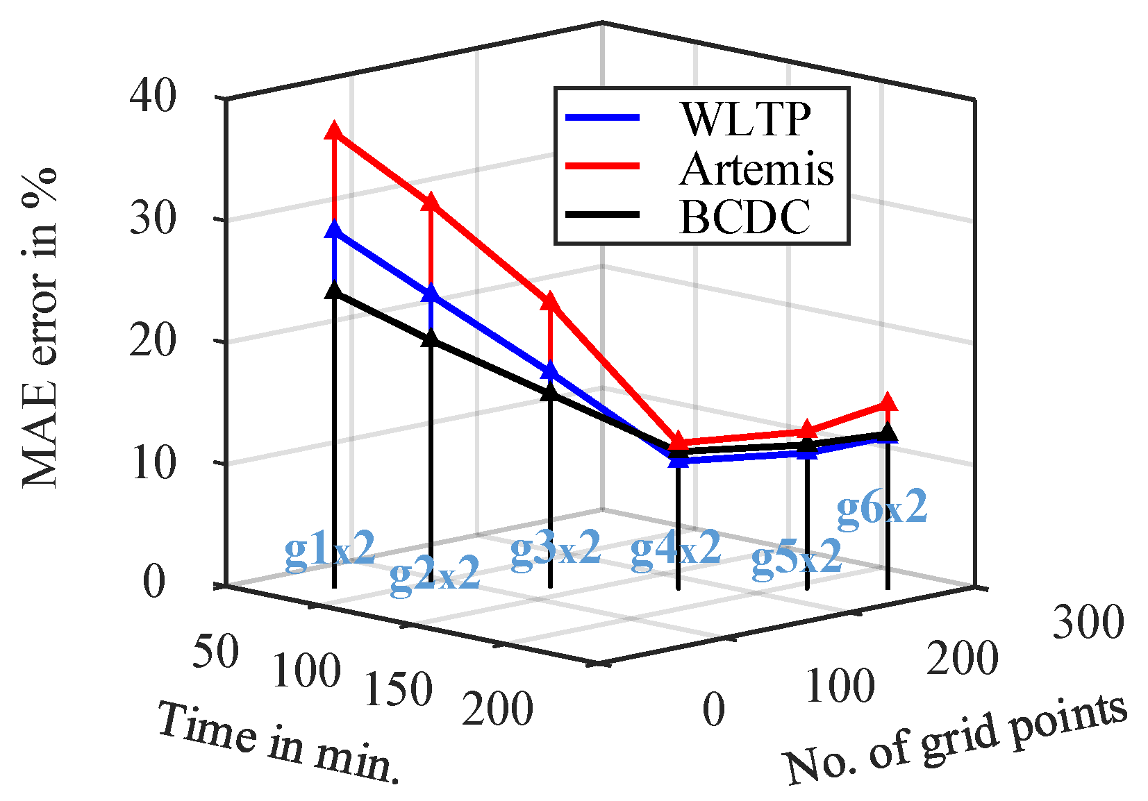
Several PMSM OPs are simulated using the FEA model with varying mesh element sizes, and the corresponding motor performance metrics are computed. These simulation results are then compared with the corresponding experimental measurements. Each simulation is performed over one full electrical period. As shown in the Figure 13, the figure illustrates the impact of mesh element size on the PMSM performance accuracy for an example operating point at 0.042 Nm and 1800 rpm. The error is presented relative to the corresponding laboratory measurements. As observed, there is a clear trade-off between accuracy and computational time: smaller mesh elements improve accuracy but increase computation time. Notably, the relationship among mesh size, accuracy, and computational effort is non-linear, highlighting the need for careful mesh-size selection to achieve better time-accuracy metrics. Moreover, Figure 14 illustrates the relationship between torque-speed grid density and time-accuracy trade-offs for various FEA-simulated grid resolutions, comparing efficiency map based drive cycles performance predictions to direct time-stepping measurements. As shown, a clear trade-off exists between computational time and accuracy, with an optimal grid density giving the best performance metrics for all drive cycles.
Figure 13.
Quantification of the FEA model in terms of mesh size, computational time, and accuracy for evaluating the performance of a PMSM OP. The results are obtained from simulations at an OP with a torque of 0.042 Nm and a speed of 1800 rpm.
Figure 13.
Quantification of the FEA model in terms of mesh size, computational time, and accuracy for evaluating the performance of a PMSM OP. The results are obtained from simulations at an OP with a torque of 0.042 Nm and a speed of 1800 rpm.
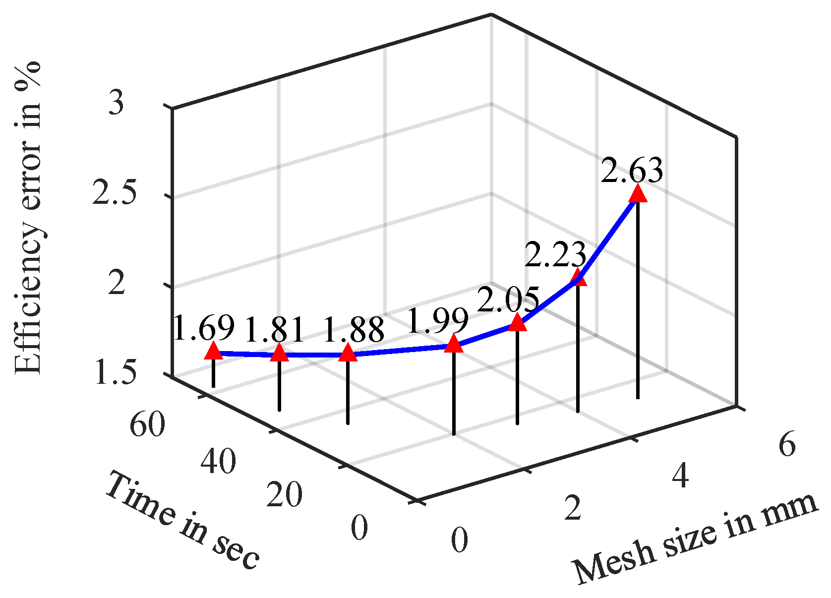
Figure 14.
Trade-off between no. of evenly spaced FEA simulated grid points ( grid×2 meaning motoring/generating regions respectively ) for efficiency map determination, simulation time and drive cycle efficiency prediction. Results are shown in terms of the MAE [47] where reference is the direct time-stepping laboratory measurements for corresponding down-scaled drive cycles (with BMW i3).
3.4.3. Quantification on Effect of Temperature
The effect of temperature on the PMSM efficiency map ( and ultimately on the drive cycles performance prediction ) is simulated and analyzed. As shown in Figure 15, increasing the steady-state temperature mainly impacts the medium to high torque-speed regions, making the map appear as if it expands from bottom to top as temperature increases. Regarding the effect on drive cycles performance, as all down-scaled drive cycles OPs of the PMSM lie in low torque regions ( typically below 50% of maximum torque ), these effects are negligible. Performance comparisons of these down-scaled drive cycles using simulated efficiency maps across different temperatures show minimal variation, with degradation from 20 °C to 100 °C being less than 0.5%. Shown in Figure 16 are the temperature rise of different motor parts during laboratory testing of the down-scaled WLTP drive cycle (with BMW i3). As observed, the temperature rise was significantly lower, indicating low thermal utilization due to the down-scaling to smaller laboratory settings.
3.4.4. Computational Efficiency of Methods
To study the computational efficiency of the efficiency map based approach, the total computational time of different methods ( Analytic, FEA, Experiment ) is considered. It includes simulation/ measurement time for an example grid density (g4), efficiency map creation, and drive cycles performance calculation. For direct time-stepping measurements, it includes the total time required for measurements and drive cycles performance calculation. This is summarized in Table 1. Efficiency map based approach is fast and can be accurate enough given the optimal grid density as well as grid points placement. Direct time-stepping measurement approach on the other hand can be time-consuming though inherently accurate.
3.4.5. Influence of Error Sources
As the study shows, irrespective of the specific method applied, the efficiency map-based steady-state approach consistently overestimates the total input energy required over a drive cycle, resulting in an artificially optimistic assessment of energy efficiency for the example case PMSM. This overestimation stems mainly from various source of errors as presented in Table 2. It neglects dynamic drive behavior and relies on linear interpolation, which seems to be the dominant source of error along with inaccurate loss modeling ( mainly mechanical losses ).
Additionally, in both steady-state based FEA and experiment approach, there are differences between the measured or simulated OPs and the reference OPs as shown in Figure 17. This also contributed to inaccurate drive cycle performance prediction due to added interpolation errors. This is the reason why g6 is found to be the optimal grid density in case of steady-sate measurement method while it is g4 for Analytic and FEA methods. The root mean squared (RMS) torque error () relative to reference grid points (g6) is 0.0020 Nm with corresponding FEA simulated points, while it is 0.0031 Nm with corresponding measured points. This difference resulted in a drive cycle performance prediction error of less than 1% in FEA and and approximately 2 to 5% for steady-state measurements when compared with direct time-stepping measurements.
4. Conclusions
This study presents a comprehensive study on the drive cycles performance analysis of a small laboratory-scale PMSM using two distinct approaches. Analytic, FEA, and experimental steady-state efficiency map based methods are studied against direct laboratory time-stepping measurements for several down-scaled drive cycles.
The findings indicate that most discrepancies between the efficiency map-based predictions and time-stepping measurements occur in low-speed regions with low-to-high torque and at high speeds with low torque. Notably, the steady-state map approach consistently overestimates the required energy input across all tested grid densities and drive cycles. Although increasing grid density improves prediction accuracy, there exists an optimal combination of grid density and grid distribution that provides the most accurate results.
Additionally, the distribution of grid points affects performance predictions, with variations of up to one-third depending on the grid configuration. Among the sources of modeling errors, grid interpolation errors are identified as the primary contributor. These errors are influenced both by the distribution of grid points and by the misalignment between simulated or measured data points and the reference points. Thermal effects are considered negligible in this study due to the down-scaling of drive cycles for such small laboratory setups.
Finally, efficiency map based approach can still be accurate enough provided that an optimal grid density or grid combination is properly simulated or measured. On the other hand, direct time-stepping measurements are resource-intensive though inherently accurate. A promising way forward lies in data-driven or high-fidelity hybrid models, that are accurate and computationally efficient.
Author Contributions
Conceptualization, P.K.D., K.H., and A.M.; Measurements, P.K.D. and R.S.; Investigation and Validation, P.K.D and K.H.; Writing—original draft, P.K.D; Supervision, A.M.; All authors have read and agreed to the published version of the manuscript.
Funding
This work is partially supported by the joint Collaborative Research Centre CREATOR (DFG: Project-ID 492661287/TRR 361; FWF: 10.55776/F90) at TU Darmstadt, TU Graz and JKU Linz. For the purpose of open access, the author has applied a CC BY public copyright license to any Author Accepted Manuscript version arising from this submission.
Data Availability Statement
A complete set of PMSM data package that provides all the required information in terms of design parameters (electrical, mechanical, geometry, windings, materials etc.) and measurement results (no-load, load and different transient drive cycles) are published with open access and available in [36].
Acknowledgments
ChatGPT 3.5 [48] has been used for editing and grammar enhancement of the paper. The paper has been subsequently edited manually again.
Conflicts of Interest
The authors declare no conflicts of interest.
Appendix A

Table A1.
The MAE [47] error of efficiencies of the PMSM drive cycles OPs obtained from steady-state efficiency maps as compared to direct time-stepping measurements. Grid densities highlighted in blue represent the optimal configurations, yielding minimal error among the grid densities evaluated.
Table A1.
The MAE [47] error of efficiencies of the PMSM drive cycles OPs obtained from steady-state efficiency maps as compared to direct time-stepping measurements. Grid densities highlighted in blue represent the optimal configurations, yielding minimal error among the grid densities evaluated.
| MAE of drive cycles OPs | ||||
| Approach | Grid | WLTP | Artemis | BCDC |
| Mid Sized Vehicle (BMW i3) | ||||
| Eff. map (analytic) | g1 | 28.08% | 35.96% | 22.91% |
| g2 | 22.86% | 30.00% | 18.97% | |
| g3 | 16.20% | 21.37% | 14.48% | |
| g4 | 8.40% | 10.00% | 9.73% | |
| g5 | 9.14% | 10.95% | 10.25% | |
| g6 | 10.68% | 13.18% | 11.28% | |
| Eff. map (FEA) | g1 | 28.76% | 36.87% | 23.58% |
| g2 | 23.35% | 30.82% | 19.48% | |
| g3 | 16.46% | 22.12% | 14.76% | |
| g4 | 8.41% | 9.65% | 9.73% | |
| g5 | 9.16% | 10.71% | 10.29% | |
| g6 | 10.14% | 11.98% | 11.00% | |
| Eff. map (experiment) | g1 | 31.69% | 39.47% | 25.32% |
| g2 | 26.08% | 33.05% | 21.22% | |
| g3 | 20.05% | 24.32% | 17.13% | |
| g4 | 12.30% | 10.09% | 12.97% | |
| g5 | 12.50% | 10.25% | 12.98% | |
| g6 | 18.89% | 10.57% | 11.50% | |
| Small Sized Vehicle (Smart EQ) | ||||
| Eff. map (analytic) | g1 | 27.09% | 33.35% | 21.88% |
| g2 | 22.13% | 26.50% | 18.02% | |
| g3 | 16.26% | 16.56% | 13.68% | |
| g4 | 10.13% | 6.11% | 9.25% | |
| g5 | 10.68% | 6.65% | 9.73% | |
| g6 | 11.85% | 8.26% | 10.66% | |
| Eff. map (FEA) | g1 | 27.77% | 34.45% | 22.49% |
| g2 | 22.60% | 27.48% | 18.45% | |
| g3 | 16.62% | 17.46% | 13.84% | |
| g4 | 10.44% | 5.72% | 9.30% | |
| g5 | 10.97% | 6.34% | 9.80% | |
| g6 | 12.14% | 8.32% | 10.77% | |
| Eff. map (experiment) | g1 | 30.66% | 36.70% | 24.14% |
| g2 | 25.25% | 29.09% | 20.10% | |
| g3 | 19.87% | 18.73% | 16.15% | |
| g4 | 13.11% | 7.64% | 12.25% | |
| g5 | 13.32% | 7.25% | 12.13% | |
| g6 | 18.70% | 17.76% | 16.21% | |
Table A2.
PMSM drive cycles energy efficiencies () obtained from grid based efficiency maps and direct time-stepping measurements. Drive cycles total output energy () as measured in the laboratory : = , = , and = . Highlighted in blue are the corresponding optimal grid densities.
Table A2.
PMSM drive cycles energy efficiencies () obtained from grid based efficiency maps and direct time-stepping measurements. Drive cycles total output energy () as measured in the laboratory : = , = , and = . Highlighted in blue are the corresponding optimal grid densities.
| Drive cycles energy efficiency | ||||
| Approach | Grid | WLTP | Artemis | BCDC |
| Small Sized Vehicle (Smart EQ) | ||||
| Time-stepping meas. | - | 56.54% | 65.84% | 39.06% |
| Eff. map (analytic) | g1 | 16.54% | 27.00% | 10.90% |
| g2 | 21.10% | 33.96% | 14.02% | |
| g3 | 28.30% | 45.62% | 19.53% | |
| g4 | 40.40% | 59.40% | 29.00% | |
| g5 | 38.62% | 58.63% | 27.80% | |
| g6 | 36.10% | 56.43% | 25.53% | |
| Eff. map (FEA) | g1 | 15.81% | 25.80% | 10.38% |
| g2 | 20.35% | 32.78% | 13.50% | |
| g3 | 27.72% | 44.50% | 19.11% | |
| g4 | 40.68% | 60.30% | 29.41% | |
| g5 | 39.05% | 59.36% | 28.04% | |
| g6 | 35.84% | 56.56% | 25.57% | |
| Eff. map (experiment) | g1 | 13.24% | 22.77% | 7.35% |
| g2 | 16.19% | 29.96% | 9.24% | |
| g3 | 22.09% | 41.61% | 12.78% | |
| g4 | 35.32% | 60.60% | 19.95% | |
| g5 | 34.73% | 59.26% | 19.54% | |
| g6 | 25.13% | 42.57% | 13.35% | |
Table A3.
PMSM drive cycles loss energies () obtained from grid based efficiency maps using different methods. Drive cycles total output energy () as measured in the laboratory : = , = , and = . Highlighted in blue are the corresponding optimal grid densities.
Table A3.
PMSM drive cycles loss energies () obtained from grid based efficiency maps using different methods. Drive cycles total output energy () as measured in the laboratory : = , = , and = . Highlighted in blue are the corresponding optimal grid densities.
| Drive cycles energy loss in kJ | ||||
| Approach | Grid | WLTP | Artemis | BCDC |
| Small Sized Vehicle (Smart EQ) | ||||
| Time-stepping meas. | - | 2.67 kJ | 3.54 kJ | 2.82 kJ |
| Eff. map (analytic) | g1 | 17.50 kJ | 18.48 kJ | 14.80 kJ |
| g2 | 13.01 kJ | 13.30 kJ | 11.08 kJ | |
| g3 | 8.80 kJ | 8.14 kJ | 6.05 kJ | |
| g4 | 5.13 kJ | 4.67 kJ | 4.43 kJ | |
| g5 | 5.50 kJ | 4.82 kJ | 4.70 kJ | |
| g6 | 6.15 kJ | 5.27 kJ | 5.26 kJ | |
| Eff. map (FEA) | g1 | 18.47 kJ | 19.65 kJ | 15.60 kJ |
| g2 | 13.58 kJ | 14.01 kJ | 11.57 kJ | |
| g3 | 9.05 kJ | 8.52 kJ | 7.65 kJ | |
| g4 | 5.06 kJ | 4.50 kJ | 4.33 kJ | |
| g5 | 5.41 kJ | 4.67 kJ | 4.63 kJ | |
| g6 | 6.21 kJ | 5.24 kJ | 5.26 kJ | |
| Eff. map (experiment) | g1 | 22.73 kJ | 23.17 kJ | 22.76 kJ |
| g2 | 17.95 kJ | 15.97 kJ | 17.75 kJ | |
| g3 | 12.23 kJ | 9.59 kJ | 12.33 kJ | |
| g4 | 6.35 kJ | 4.44 kJ | 7.25 kJ | |
| g5 | 6.52 kJ | 4.70 kJ | 7.43 kJ | |
| g6 | 10.33 kJ | 9.22 kJ | 11.72 kJ | |
References
- Blanco, S. Toyota, Mazda, Subaru agree carbon is ‘enemy’ with internal combustion engine announcement, 2024. SAE International, Available at: https://www.sae.org/site/news/2024/05/toyota-internal-combustion-future-engines (Accessed: 2025-09-08).
- Rémont, L. Why electrification is so important to the energy transition, 2025. World Economic Forum, Available at: https://www.weforum.org/stories/2025/01/why-electrification-important-energy-transition/ (Accessed: 2025-09-08).
- Liu, C.; Chau, K.T.; Lee, C.H.T.; Song, Z. A Critical Review of Advanced Electric Machines and Control Strategies for Electric Vehicles. Proceedings of the IEEE 2021, 109, 1004–1028. [CrossRef]
- Sayed, E.; Abdalmagid, M.; Pietrini, G.; Sa’adeh, N.M.; Callegaro, A.D.; Goldstein, C.; Emadi, A. Review of Electric Machines in More-/Hybrid-/Turbo-Electric Aircraft. IEEE Transactions on Transportation Electrification 2021, 7, 2976–3005. [CrossRef]
- Huynh, T.A.; Chen, P.H.; Hsieh, M.F. Analysis and Comparison of Operational Characteristics of Electric Vehicle Traction Units Combining Two Different Types of Motors. IEEE Transactions on Vehicular Technology 2022, 71, 5727–5742. [CrossRef]
- Pyrhönen, J.; Jokinen, T.; Hrabovcová, V. Design of Rotating Electrical Machines; Wiley: USA, 2013.
- Grunditz, E.A.; Thiringer, T.; Saadat, N. Acceleration, Drive Cycle Efficiency, and Cost Tradeoffs for Scaled Electric Vehicle Drive System. IEEE Transactions on Industry Applications 2020, 56, 3020–3033. [CrossRef]
- Ozer, K.; Yilmaz, M. Design and Optimization of IPMSM for Enhanced Efficiency, Cost Reduction, and Performance in Light Electric Vehicles. IEEE Access 2025, 13, 80621–80636. [CrossRef]
- Fatemi, A.; Demerdash, N.A.O.; Nehl, T.W.; Ionel, D.M. Large-Scale Design Optimization of PM Machines Over a Target Operating Cycle. IEEE Transactions on Industry Applications 2016, 52, 3772–3782. [CrossRef]
- Diao, K.; Sun, X.; Lei, G.; Bramerdorfer, G.; Guo, Y.; Zhu, J. System-Level Robust Design Optimization of a Switched Reluctance Motor Drive System Considering Multiple Driving Cycles. IEEE Transactions on Energy Conversion 2021, 36, 348–357. [CrossRef]
- Praslicka, B.; Ma, C.; Taran, N. A Computationally Efficient High-Fidelity Multi-Physics Design Optimization of Traction Motors for Drive Cycle Loss Minimization. IEEE Transactions on Industry Applications 2023, 59, 1351–1360. s. [CrossRef]
- Roshandel, E.; Mahmoudi, A.; Soong, W.L.; Kahourzade, S. Optimal Design of Induction Motors Over Driving Cycles for Electric Vehicles. IEEE Transactions on Vehicular Technology 2023, 72, 15548–15562. [CrossRef]
- Hwang, S.W.; Ryu, J.Y.; Chin, J.W.; Park, S.H.; Kim, D.K.; Lim, M.S. Coupled Electromagnetic-Thermal Analysis for Predicting Traction Motor Characteristics According to Electric Vehicle Driving Cycle. IEEE Transactions on Vehicular Technology 2021, 70, 4262–4272. [CrossRef]
- Fan, D.; Zhu, X.; Quan, L.; Han, P.; Xiang, Z.; Wu, J. Driving Cycle Design Optimization of Less-Rare-Earth PM Motor Using Dimension Reduction Method. IEEE Transactions on Energy Conversion 2023, 38, 1614–1625. Conference Name: IEEE Transactions on Energy Conversion. [CrossRef]
- Abdel-Wahed, A.T.; Ullah, Z.; Abdel-Khalik, A.S.; Hamad, M.S.; Ahmed, S.; Elmalhy, N. Drive Cycle-Based Design With the Aid of Data Mining Methods: A Review on Clustering Techniques of Electric Vehicle Motor Design With a Case Study. IEEE Access 2023, 11, 115775–115797. [CrossRef]
- Mahmouditabar, F.; Vahedi, A.; Takorabet, N. Robust Design of BLDC Motor Considering Driving Cycle. IEEE Transactions on Transportation Electrification 2024, 10, 1414–1424. [CrossRef]
- Bhaktha, B.S.; Jose, N.; Vamshik, M.; Pitchaimani, J.; Gangadharan, K.V. Driving Cycle-Based Design Optimization and Experimental Verification of a Switched Reluctance Motor for an E-Rickshaw. IEEE Transactions on Transportation Electrification 2024, 10, 9959–9974. [CrossRef]
- Mahmouditabar, F.; Vahedi, A.; Takorabet, N. Robust Design of BLDC Motor Considering Driving Cycle. IEEE Transactions on Transportation Electrification 2024, 10, 1414–1424. [CrossRef]
- Williamson, S.S.; Emadi, A.; Rajashekara, K. Comprehensive Efficiency Modeling of Electric Traction Motor Drives for Hybrid Electric Vehicle Propulsion Applications. IEEE Trans. Veh. Technol. 2007, 56, 1561–1572. [CrossRef]
- Jun, S.B.; Kim, C.H.; Cha, J.; Lee, J.H.; Kim, Y.J.; Jung, S.Y. A Novel Method for Establishing an Efficiency Map of IPMSMs for EV Propulsion Based on the Finite-Element Method and a Neural Network. Electronics 2021, 10. [CrossRef]
- Roshandel, E.; Mahmoudi, A.; Kahourzade, S.; Soong, W.L. Efficiency Maps of Electrical Machines: A Tutorial Review. IEEE Transactions on Industry Applications 2023, 59, 1263–1272. [CrossRef]
- Ferrari, S.; Ragazzo, P.; Dilevrano, G.; Pellegrino, G. Flux and Loss Map Based Evaluation of the Efficiency Map of Synchronous Machines. IEEE Transactions on Industry Applications 2023, 59, 1500–1509. [CrossRef]
- Stiscia, O.; Rubino, S.; Vaschetto, S.; Cavagnino, A.; Tenconi, A. Accurate Induction Machines Efficiency Mapping Computed by Standard Test Parameters. IEEE Trans. on Ind. Applicat. 2022, 58, 3522–3532.
- Bojoi, R.; Armando, E.; Pastorelli, M.; Lang, K. Efficiency and loss mapping of AC motors using advanced testing tools. In Proceedings of the 2016 XXII International Conference on Electrical Machines (ICEM), sep 2016, pp. 1043–1049. [CrossRef]
- Dhakal, P.K.; Heidarikani, K.; Seebacher, R.; Muetze, A. Baseline Determination for Drive Cycle Performance Analysis of Permanent Magnet Synchronous Motors. In Proceedings of the 2023 IEEE Transportation Electrification Conference and Expo, Asia-Pacific (ITEC Asia-Pacific), Chiang Mai, Thailand, nov 2023; pp. 1–6. [CrossRef]
- Heidarikani, K.; Dhakal, P.K.; Seebacher, R.; Muetze, A. Baseline Determination for Drive Cycle Performance Analysis of Induction Motors. In Proceedings of the 2023 IEEE Transportation Electrification Conference and Expo, Asia-Pacific (ITEC Asia-Pacific), nov 2023, pp. 1–6. [CrossRef]
- Kahourzade, S.; Mahmoudi, A.; Soong, W.L.; Ertugrul, N.; Pellegrino, G. Estimation of PM Machine Efficiency Maps From Limited Data. IEEE Transactions on Industry Applications 2020, 56, 2612–2621. [CrossRef]
- Sano, H.; Semba, K.; Suzuki, Y.; Yamada, T. Investigation in the accuracy of FEA Based Efficiency Maps for PMSM traction machines. In Proceedings of the 2022 International Conference on Electrical Machines (ICEM), Valencia, Spain, sep 2022; pp. 2061–2066.
- Mohammadi, M.H.; Lowther, D.A. A Computational Study of Efficiency Map Calculation for Synchronous AC Motor Drives Including Cross-Coupling and Saturation Effects. IEEE Transactions on Magnetics 2017, 53, 1–4. [CrossRef]
- Mahmouditabar, F.; Baker, N.J. Design Optimization of Induction Motors with Different Stator Slot Rotor Bar Combinations Considering Drive Cycle. Energies 2024, 17, 154. Number: 1 Publisher: Multidisciplinary Digital Publishing Institute. [CrossRef]
- Gong, Y.; Gneiting, A.; Weigel, S.; Parspour, N.; An, Z. Surrogate Model Based Drive Cycle Modelling and Optimization of Synchronous Reluctance Machines for Electric Vehicles. IEEE Transactions on Magnetics 2025, pp. 1–1. [CrossRef]
- Farajpour, Y.; Chaoui, H.; Kelouwani, S. Cutting-Edge EMS Technologies for EVs and HEVs: Recent Developments and Future Directions. IEEE Access 2025, pp. 1–1. [CrossRef]
- Narita, K.; Sano, H.; Schneider, N.; Semba, K.; Tani, K.; Yamada, T.; Akaki, R. An Accuracy Study of Finite Element Analysis-based Efficiency Map for Traction Interior Permanent Magnet Machines. In Proceedings of the 2020 IEEE Energy Conversion Congress and Exposition (ECCE), Detroit, MI, USA, oct 2020; pp. 1722–1726.
- Dhakal, P.K.; Heidarikani, K.; Seebacher, R.; Muetze, A. Efficiency Map Versus Time-Stepping Solutions for Drive Cycle Performance Analysis of Permanent Magnet Synchronous Motors. In Proceedings of the 2024 27th International Conference on Electrical Machines and Systems (ICEMS), 2024, pp. 336–340. [CrossRef]
- Heidarikani, K.; Dhakal, P.K.; Seebacher, R.; Muetze, A. Quantification of Steady-State Efficiency Maps and Time-Stepping Solutions for Drive Cycle Performance Analysis of Induction Motors. In Proceedings of the 2024 27th International Conference on Electrical Machines and Systems (ICEMS), Fukuoka, Japan, nov 2024; pp. 1–6.
- Dhakal, P.K.; Heidarikani, K.; Muetze, A.; Seebacher, R. CREATOR Case: Permanent Magnet Synchronous Motor Data, 2024. Graz University of Technology. [CrossRef]
- Dhakal, P.K.; Heidarikani, K.; Muetze, A. Down-scaling of drive cycles for experimental drive cycle analyses. In Proceedings of the 12th International Conference on Power Electronics, Machines and Drives (PEMD 2023), Brussels, Belgium, oct 2023; Vol. 2023, pp. 271–276. [CrossRef]
- Vanhooydonck, D.; Symens, W.; Deprez, W.; Lemmens, J.; Stockman, K.; Dereyne, S. Calculating energy consumption of motor systems with varying load using iso efficiency contours. In Proceedings of the The XIX International Conference on Electrical Machines - ICEM 2010, sep 2010, pp. 1–6. [CrossRef]
- Cheng, Y.; Wang, Y.; Ma, J.; Liu, G.; Li, D.; Qu, R. Fast Evaluation of Driving Cycle Efficiency of Interior Permanent Magnet Synchronous Machines for Electric Vehicles Considering Step-Skewing. In Proceedings of the 2023 IEEE International Electric Machines & Drives Conference (IEMDC), may 2023, pp. 1–7. [CrossRef]
- Praslicka, B.; Taran, N.; Ma, C. An Ultra-fast Method for Analyzing IPM Motors at Multiple Operating Points Using Surrogate Models. In Proceedings of the 2022 IEEE Transportation Electrification Conference & Expo (ITEC), 2022, pp. 868–873. [CrossRef]
- Kong, Y.; Nicola, B.; Lin, M. Loss Functions and Efficiency Model of Permanent Magnet Assisted Synchronous Reluctance Machine. IEEE Transactions on Energy Conversion 2023, 38, 53–63. [CrossRef]
- Roshandel, E.; Mahmoudi, A.; Kahourzade, S.; Yazdani, A.; Shafiullah, G.M. Losses in Efficiency Maps of Electric Vehicles: An Overview. Energies 2021, 14, 7805. [CrossRef]
- Bertotti, G. Hysteresis in Magnetism: For Physicists, Materials Scientists, and Engineers; Academic Press, 1998.
- MathWorks. Curve Fitting Toolbox, 2025. Available at: https://www.mathworks.com/products/curvefitting.html (Accessed: 2025-09-08).
- JSOL. Simulation Technology for Electromechanical Design : JMAG. Available at: https://www.jmag-international.com/ (Accessed: 2025-09-08).
- HBK. "eDrive Power Analyzer, 6CH, 2MS/s, GEN3iA". Available at: https://www.hbkworld.com/en/products/instruments/power-analyser/edrive/1-edrv-6p-3i (Accessed: 2025-09-08).
- Wikipedia. Mean absolute error, 2025. Available at: https://en.wikipedia.org/wiki/Mean_absolute_error (Accessed: 2025-09-08).
- OpenAI. ChatGPT 4-o. Available at: https://chatgpt.com/ (Accessed: 2025-09-08).
Figure 1.
Flowchart of the study.
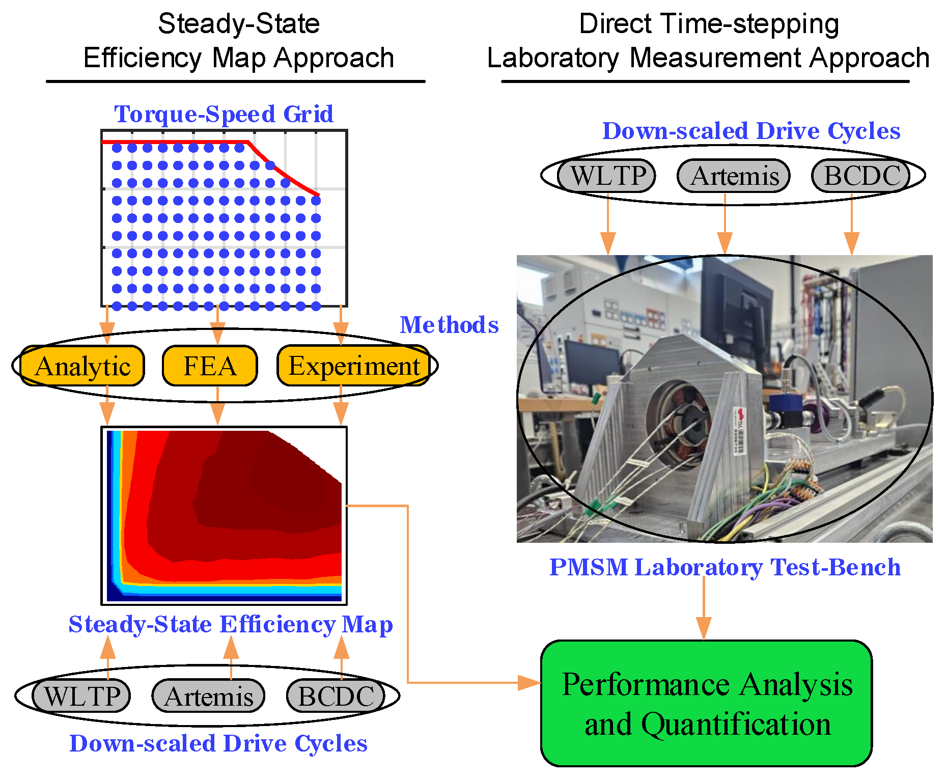
Figure 2.
Different torque-speed grid densities considered for the efficiency map based analysis.
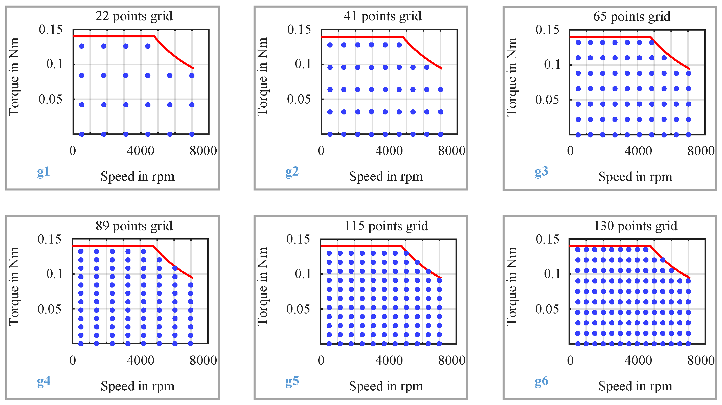
Figure 3.
A 2D schematic of the PMSM FEA model.
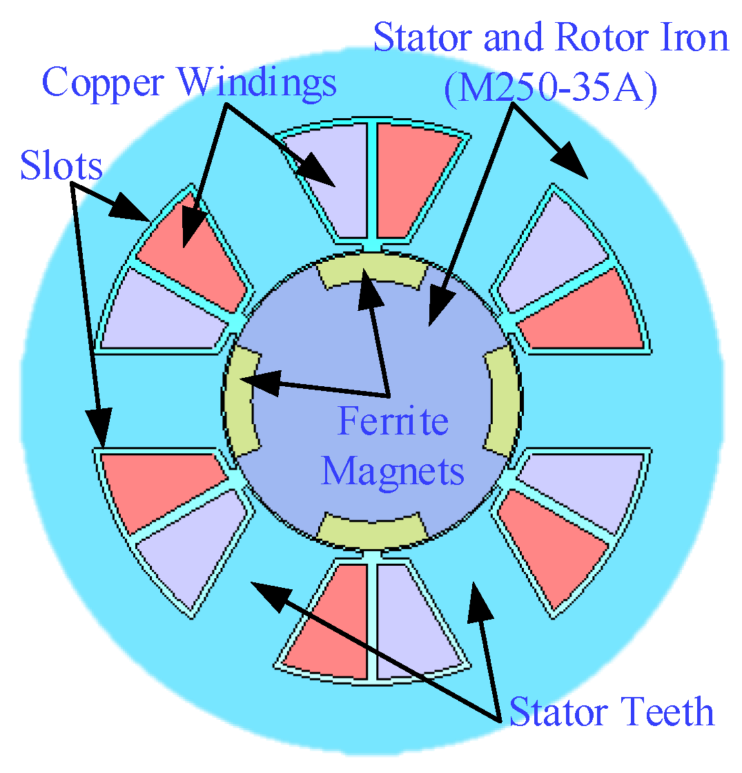
Figure 4.
A 3D schematic of the PMSM laboratory test bench. The orange lines represent the simplified control schematic. The system integrates both efficiency map-based computations and direct time-stepping laboratory measurements. The motor under test is torque controlled and the load motor is speed controlled.
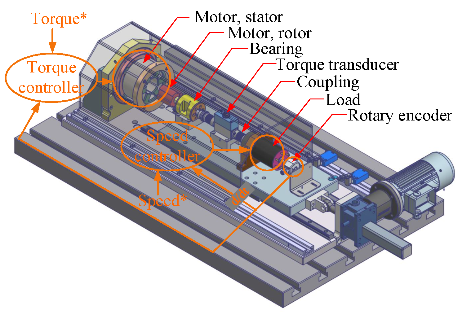
Figure 5.
Complete control block diagram of the PMSM laboratory test bench used for drive cycle time-stepping measurements. Real-time control, data acquisition, and torque-speed profile tracking are implemented to ensure accurate replication of drive scenarios. The speed in fed back using a low pass filter (LPF) with a time constant of .
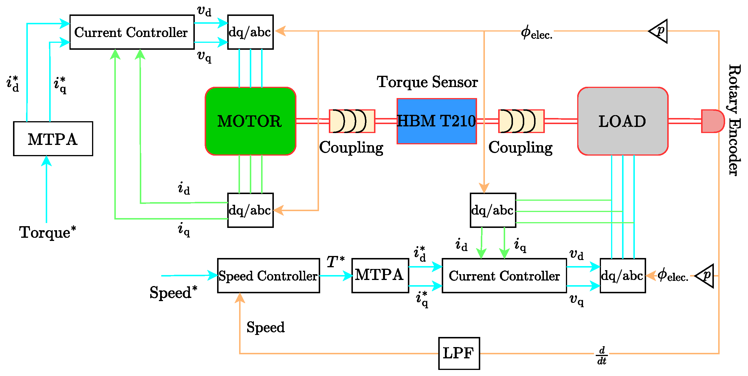
Figure 6.
Efficiency maps and corresponding efficiency plots of the PMSM during down-scaled WLTP drive cycle OPs (with BMW i3), determined from steady-state LUT based analysis through: (a) FEA model, (b) analytic model, (c) experiment; interpolations are based on the 130-points grid for each map.
Figure 6.
Efficiency maps and corresponding efficiency plots of the PMSM during down-scaled WLTP drive cycle OPs (with BMW i3), determined from steady-state LUT based analysis through: (a) FEA model, (b) analytic model, (c) experiment; interpolations are based on the 130-points grid for each map.
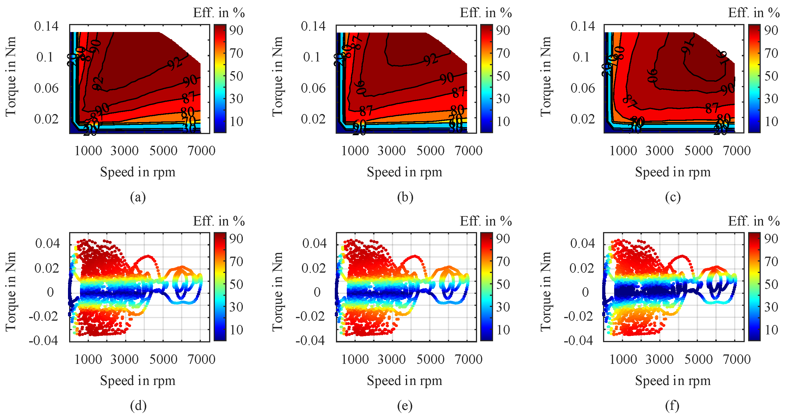
Figure 7.
Efficiency difference heat maps of torque-speed OP efficiencies determined through simulations and measurements: (a) FEA – Experiment, (b) Analytic – Experiment, (c) FEA – Analytic. The example results are shown for the 130-points grid .
Figure 7.
Efficiency difference heat maps of torque-speed OP efficiencies determined through simulations and measurements: (a) FEA – Experiment, (b) Analytic – Experiment, (c) FEA – Analytic. The example results are shown for the 130-points grid .
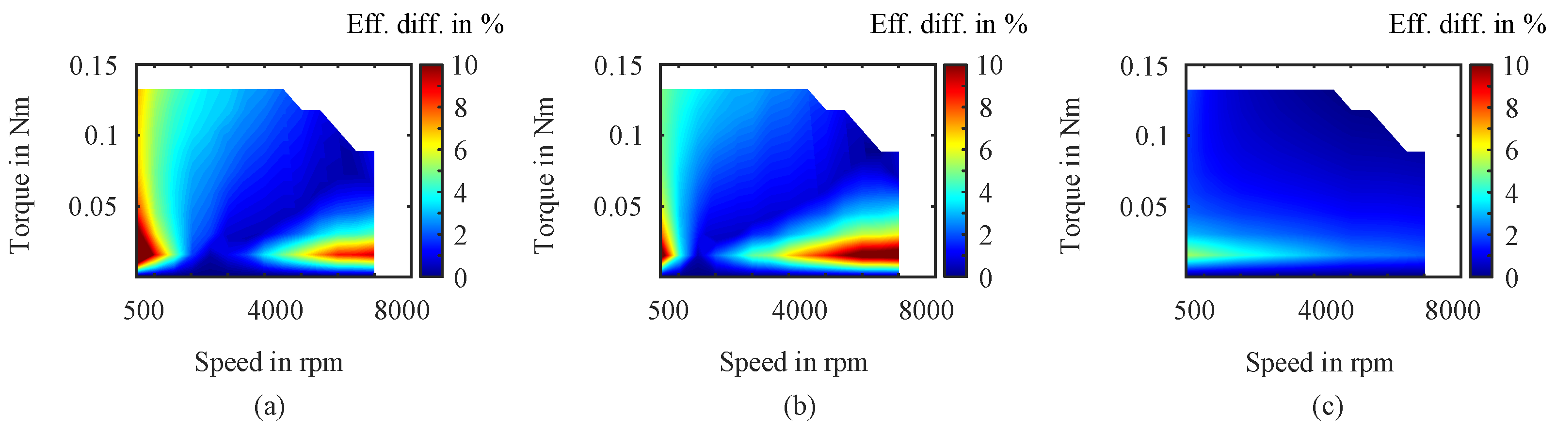
Figure 8.
Laboratory measurement results of full down-scaled WLTP drive cycle (with BMW i3): (a) speed-time profile, (b) torque-time profile, (c) input and output power-time profiles, (d) calculated efficiency-time profile.
Figure 8.
Laboratory measurement results of full down-scaled WLTP drive cycle (with BMW i3): (a) speed-time profile, (b) torque-time profile, (c) input and output power-time profiles, (d) calculated efficiency-time profile.
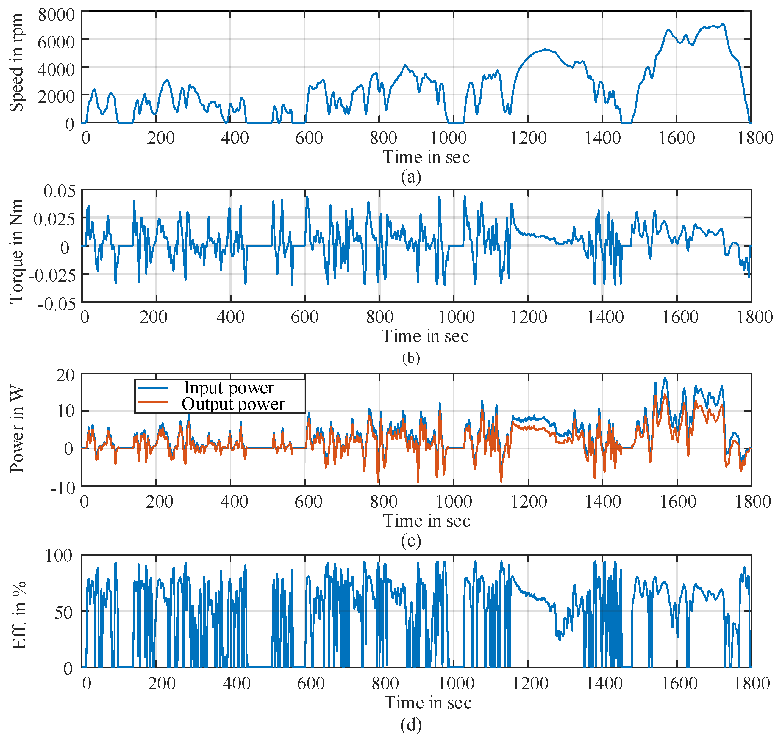
Figure 9.
Drive cycle energy conversion efficiencies from steady-state efficiency map based approach and direct laboratory time-stepping measurements . Efficiency maps as LUTs are constructed and results are shown for different torque-speed grid points ( grid×2 meaning motoring/generating regions, respectively ) using: (a) FEA method, (b) Analytic method, (c) Experiment method. Drive cycles total output energy as measured in the laboratory: WLTP = 2.96 kJ, Artemis = 5.37 kJ, and BCDC = 1.45 kJ.
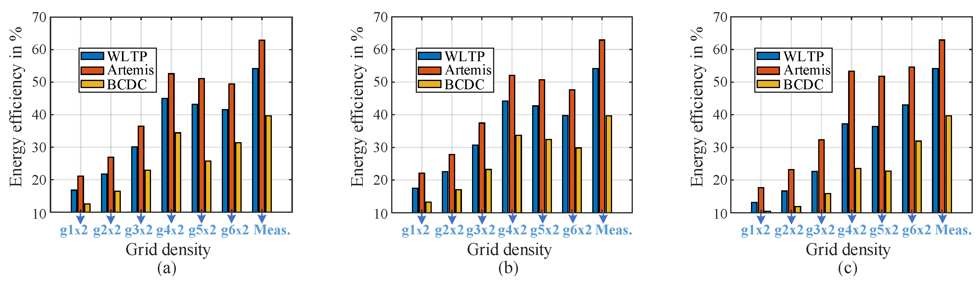
Figure 10.
Influence of the no. of grid points on the efficiency maps’ predictive performance. The figures show the energy loss of the drive cycles as determined from efficiency maps and by direct time-stepping measurements in the laboratory , all for the mid-size car (BMW i3). Efficiency maps as LUTs are constructed for different torque-speed grid points ( grid×2 meaning motoring/generating regions respectively ) using: (a) FEA method, (b) Analytic method, (c) Experiment method. Drive cycles total input energy as measured in the laboratory: WLTP = 5.46 kJ, Artemis = 8.53 kJ, and BCDC = 3.65 kJ.
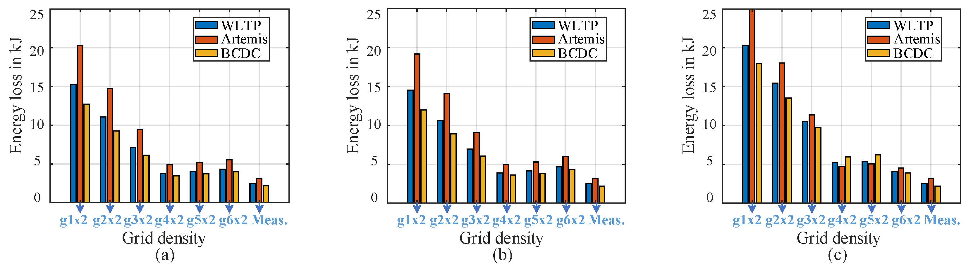
Figure 11.
Total input energy measured or simulated during down-scaled WLTP drive cycle (with BMW i3) operation using different approaches. Time-stepping analytical simulations are conducted in the MATLAB/Simulink® environment. For the steady-state efficiency map-based analysis, results are presented only for the optimal grid density identified among the grid densities evaluated.
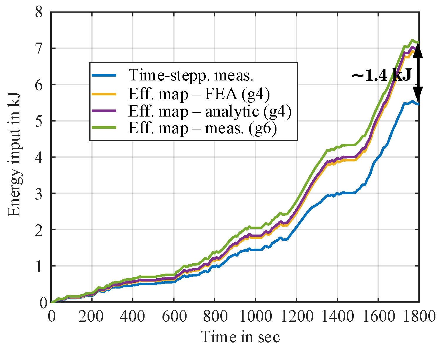
Figure 12.
Quantification of grid interpolation errors associated with torque-speed grid points under different placement strategies. Plot shows loss energies of different down-scaled drive cycles (with BMW i3), obtained from map-based analyses using various grid points placement and from direct time-stepping laboratory measurements.
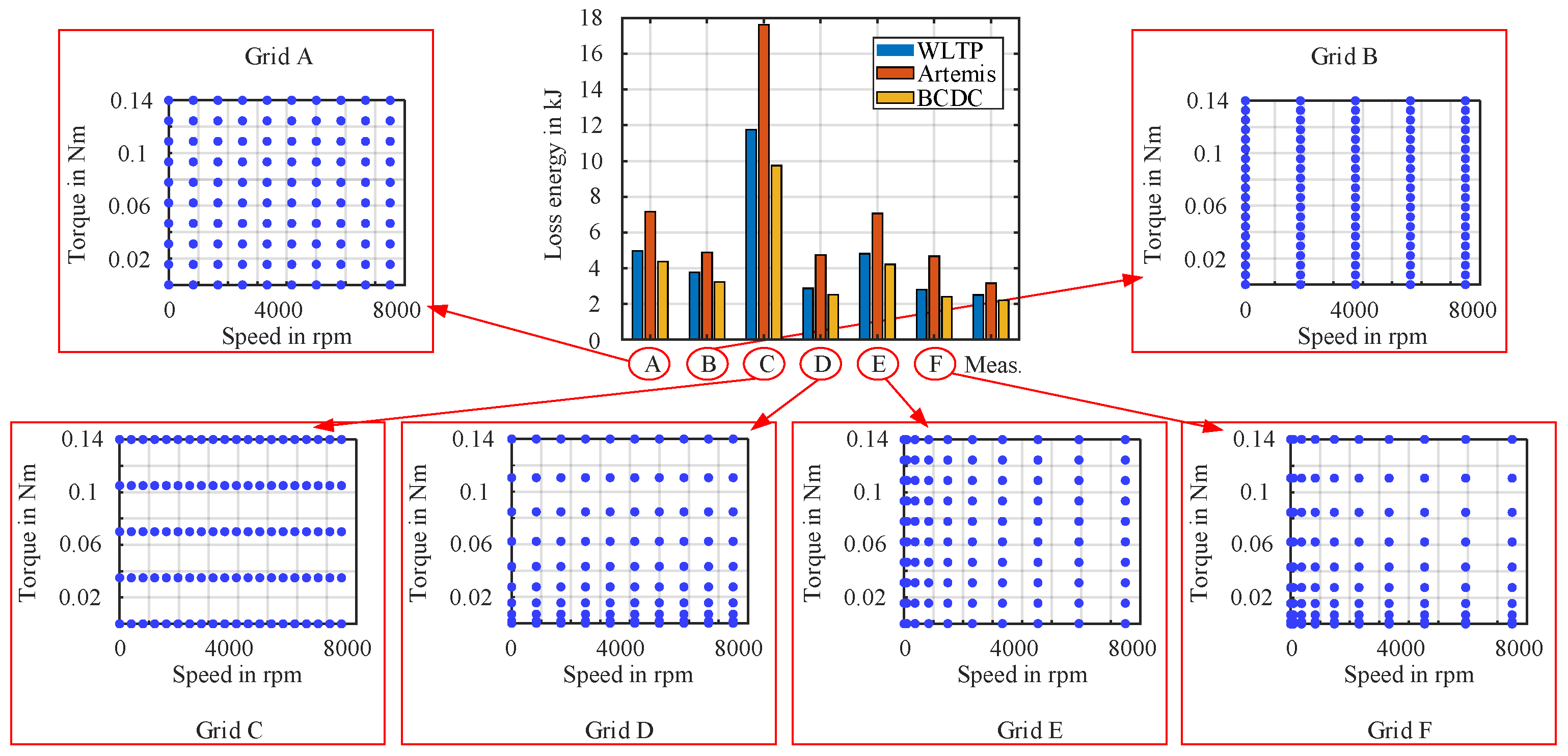
Figure 15.
Simulated steady-state efficiency maps of the PMSM at different temperatures: (a) 20 °C, (b) 100 °C; interpolations are based on the 130-points grid for each map.
Figure 15.
Simulated steady-state efficiency maps of the PMSM at different temperatures: (a) 20 °C, (b) 100 °C; interpolations are based on the 130-points grid for each map.
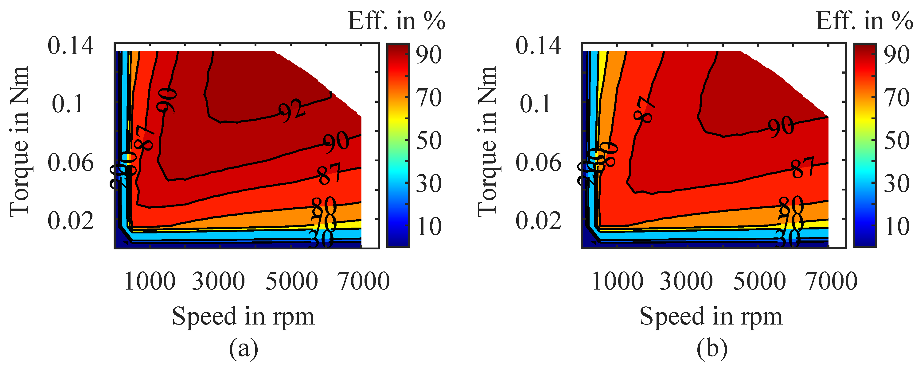
Figure 16.
Measured temperature rise (T) of selected parts of the laboratory PMSM during down-scaled WLTP drive cycle (with BMW i3) operation.
Figure 16.
Measured temperature rise (T) of selected parts of the laboratory PMSM during down-scaled WLTP drive cycle (with BMW i3) operation.
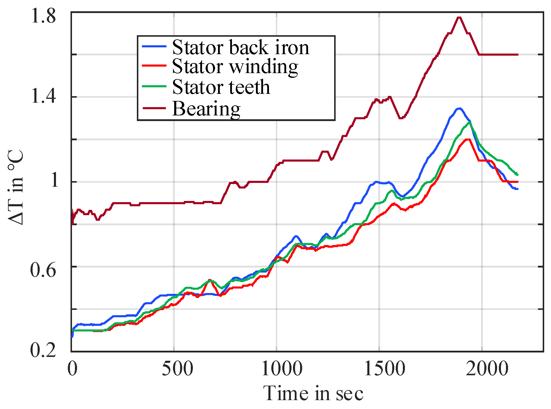
Figure 17.
Visual difference between the reference and measured/simulated torque-speed OPs for steady-state efficiency map approach with: (a) FEA method, (b) Experiment method. An example case of 130 points grid is presented.
Figure 17.
Visual difference between the reference and measured/simulated torque-speed OPs for steady-state efficiency map approach with: (a) FEA method, (b) Experiment method. An example case of 130 points grid is presented.
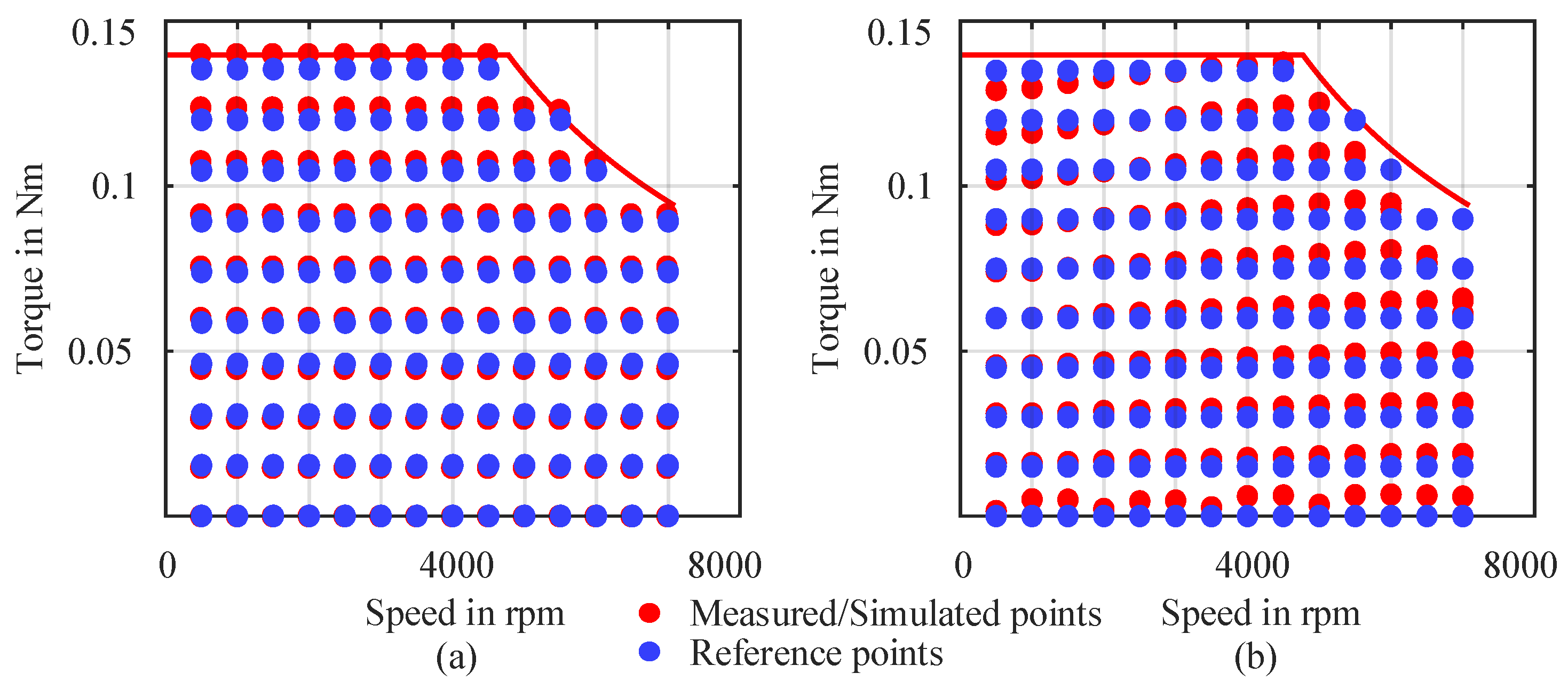
Table 1.
Simulation and measurement times of different approaches on drive cycles performance computation.
Table 1.
Simulation and measurement times of different approaches on drive cycles performance computation.
| Approach | Drive Cycles | ||
|---|---|---|---|
| WLTP | Artemis | BCDC | |
| Time-stepping meas. | ∼44 min. | ∼29 min. | ∼44 min. |
| Eff. map (analytic, g4) | <1 min. | ||
| Eff. map (FEA, g4) | ∼122 min. | ||
| Eff. map (experiment, g4) | ∼100 min. | ||
Table 2.
Impact level of error sources on drive cycle efficiency prediction using efficiency maps as LUTs across PMSM models (aggregated view).
Table 2.
Impact level of error sources on drive cycle efficiency prediction using efficiency maps as LUTs across PMSM models (aggregated view).
| Error Source | Impact Level (out of 5) |
|---|---|
| Interpolation errors in LUT based analysis |
++++ |
| Inaccurate friction and mechanical loss estimation |
+++ |
| Laboratory test-bench related unknown errors |
++ |
| Iron loss modeling inaccuracies (e.g., hysteresis, eddy currents) |
++ |
| Inaccurate motor parameters |
+ |
| Unmodeled harmonics or PWM switching effects |
+ |
| Mesh quality and resolution in FEA |
+ |
| Thermal effects and temperature dependencies |
+ |
Disclaimer/Publisher’s Note: The statements, opinions and data contained in all publications are solely those of the individual author(s) and contributor(s) and not of MDPI and/or the editor(s). MDPI and/or the editor(s) disclaim responsibility for any injury to people or property resulting from any ideas, methods, instructions or products referred to in the content. |
© 2025 by the authors. Licensee MDPI, Basel, Switzerland. This article is an open access article distributed under the terms and conditions of the Creative Commons Attribution (CC BY) license (http://creativecommons.org/licenses/by/4.0/).
Copyright: This open access article is published under a Creative Commons CC BY 4.0 license, which permit the free download, distribution, and reuse, provided that the author and preprint are cited in any reuse.


