
Submitted:
22 September 2025
Posted:
23 September 2025
You are already at the latest version
Abstract
Evaluating electric vehicle (EV) motor performance over dynamic drive cycles is essential for accurate energy efficiency prediction and system-level optimization. While conventional steady-state models enable rapid generation of efficiency maps, they can introduce significant errors due to grid interpolation and the omission of transient behavior. Limited understanding exists regarding how grid coarseness and modeling approach affect the discrepancy between steady-state and time-stepping solutions. This study quantifies these differences for a laboratory-scale induction motor (IM) operating under down-scaled drive cycles, using experimental time-stepping measurements as a reference. Efficiency maps are developed using three methods—analytic modeling, finite element analysis (FEA), and experimental testing—while time-stepping simulations are conducted using an analytic model. The study evaluates both total drive cycle energy efficiency errors and pointwise deviations across the torque-speed envelope for various grid resolutions. Results are compared against laboratory-based time-stepping measurements to identify trade-offs between computational efficiency and accuracy. Additionally, a sensitivity analysis is performed to assess the impact of operating point (OP) placement within the grid and temperature variation on the accuracy of efficiency mapping.
Keywords:
drive cycle performance
; efficiency maps
; finite element analysis (FEA)
; time-stepping solutions
; induction motor
; experimental measurements
1. Introduction
Rising energy and environmental concerns have made electric vehicles (EVs) crucial for reducing emissions and fossil fuel use [1,2,3], driving the need for improved design and optimization of EV powertrain components, especially traction motors [4]. Drive cycles play a crucial role in this process by replicating real-world driving conditions, allowing for accurate evaluation of motor performance. Standardized drive cycles simulate typical urban and highway conditions [5,6]. Evaluating motor efficiency under these scenarios helps optimize powertrain energy flow, size the battery, and reduce energy consumption [7].
Currently, the most prevalent motor topologies in EV applications are induction motors (IMs) and permanent magnet synchronous motors (PMSMs) [8,9]. While PMSMs offer high torque density and excellent low-speed efficiency, IMs stand out for their lower cost, mechanical durability, rare-earth-free design, and extended field-weakening capability. Despite drawbacks such as lower efficiency and power factor, IMs remain attractive for scalable, cost-sensitive EV platforms [10,11]. In this context, optimizing IM performance under realistic drive cycles is key to improving powertrain efficiency and enabling cost-effective, reliable EVs [12].
Motor efficiency maps illustrate electric machine performance across torque–speed points and provide a foundation for evaluating EV efficiency. These maps are typically stored as look-up tables (LUTs) and are generated using experimental measurements, finite element analysis (FEA), or analytical models under steady-state conditions [13,14,15]. LUT-based efficiency maps are computationally efficient and widely used in EV simulations [16,17,18], enabling fast evaluations of motor behavior. However, these maps neglect transients such as acceleration, deceleration, and temperature changes, leading to deviations from real drive cycle performance [19,20]. Their accuracy also depends on torque–speed grid resolution and distribution, where coarse or uneven grids can introduce systematic errors, especially under parameter uncertainty [21]. To address these limitations, hybrid approaches can combine FEA-based LUTs with analytical models to improve efficiency and capture dynamic effects, but they remain limited by LUT approximations, model assumptions, and setup complexity [22]. Data-driven methods such as machine learning and surrogate models offer speed with low data requirements but are rarely validated experimentally [6,23,24,25]. Time-stepping simulations, as a high-fidelity method, remain accurate under dynamic loading but are too computationally expensive for routine design or large-scale optimization, leaving the trade-off between fidelity and efficiency unresolved [1,26,27,28].
Given these complexities, comparing LUT-based and time-stepping methods is vital to reveal trade-offs between computational efficiency and accuracy, guiding the selection of appropriate methods for EV motor drive cycle evaluation. Despite the widespread use of steady-state LUT-based efficiency maps, a critical gap remains in understanding how modeling choices and grid density influence efficiency prediction under dynamic conditions. Most studies implement a single efficiency mapping approach without comparing its performance against alternative methods like time-stepping methods under consistent vehicle and drive cycle scenarios [13,29]. Moreover, while efficiency maps are commonly used to evaluate drive cycle performance, limited attention has been given to how torque-speed grid density, spatial placement of OPs on the grid, and motor temperature variation influence both map accuracy and the resulting drive cycle performance predictions [30,31].
Although time-stepping simulations have gained traction in recent years, they are primarily implemented at the system-level and often rely on fixed efficiency maps, without dynamically resolving motor behavior under thermal and electromagnetic transients [4,28]. Many of these efforts are rooted in theoretical modeling with limited experimental validation, further limiting their reliability in predicting real-world motor performance [32,33].
1.1. Contribution of This Paper
Two complementary research efforts have been carried out at laboratory scale: one on the IM and the other on the PMSM. Earlier conference papers presented initial results from these investigations, reported separately for each motor type [1,19,20,27]. The results presented in this paper are based on the study carried out for the IM, including comprehensive evaluation and benchmarking, while a companion manuscript covering the PMSM has been submitted separately. This separation ensures clarity for readers and highlights the motor-specific contributions of each study. This paper presents an extensive extension of the initial study introduced in [1]. It provides a comprehensive evaluation of LUT-based methods and time-stepping simulations for predicting the performance of a laboratory-scale IM under dynamic drive cycles, benchmarked against experimental time-stepping measurements. The comparison covers three standard drive cycles and two EV platforms, quantifying both drive cycle energy conversion efficiency and point-wise OP efficiency across the torque-speed trajectory for various grid resolutions and methods. The effectiveness of each approach is assessed in terms of accuracy and computational cost, highlighting key trade-offs and practical considerations. Additionally, a sensitivity analysis examines how OP placement within the torque-speed envelope and temperature variations influence efficiency mapping, offering insights for optimizing grid design and improving performance prediction.
The paper is organized as follows. Section II describes the methodology along with the modeling and experimental framework. Section III presents the results of the steady-state and direct performance analyses. Section IV quantifies errors by comparing the results with measurements, while Section V evaluates the sensitivity of the efficiency maps. Section VI discusses factors affecting accuracy and computational efficiency, and finally, Section VII concludes with a summary of the key findings.
2. Test Cases, Modeling, and Experimental Setup
2.1. Methodology and Test Case Overview
In this research, the performance of the target OPs associated with drive cycles is evaluated using both steady-state LUT methods and time-stepping simulation techniques. Three widely used standard drive cycles are considered to represent different vehicle usage scenarios: WLTP Class 3, Artemis 130 km/h (inter-city), and the Braunschweig City Driving Cycle (BCDC, urban). Their speed–time profiles are illustrated in Figure 1.The drive cycle input torque-speed OPs () are obtained from quasi-steady-state (QSS) vehicle models of the BMW i3 (mid-range) and Smart EQ (small-range), capturing a broad range of vehicle dynamics.
Specifications of both the vehicle motors and the laboratory IM are summarized in Table 1. Since the IM in the laboratory has lower torque and speed ratings than the original vehicle motors, a down-scaling procedure based on the methods in [35,36] is applied to generate OPs within the range of the laboratory IM while maintaining dynamic consistency with the original vehicle drive cycles. These OPs represent the OP of the laboratory motor and serve as inputs for the study [19].
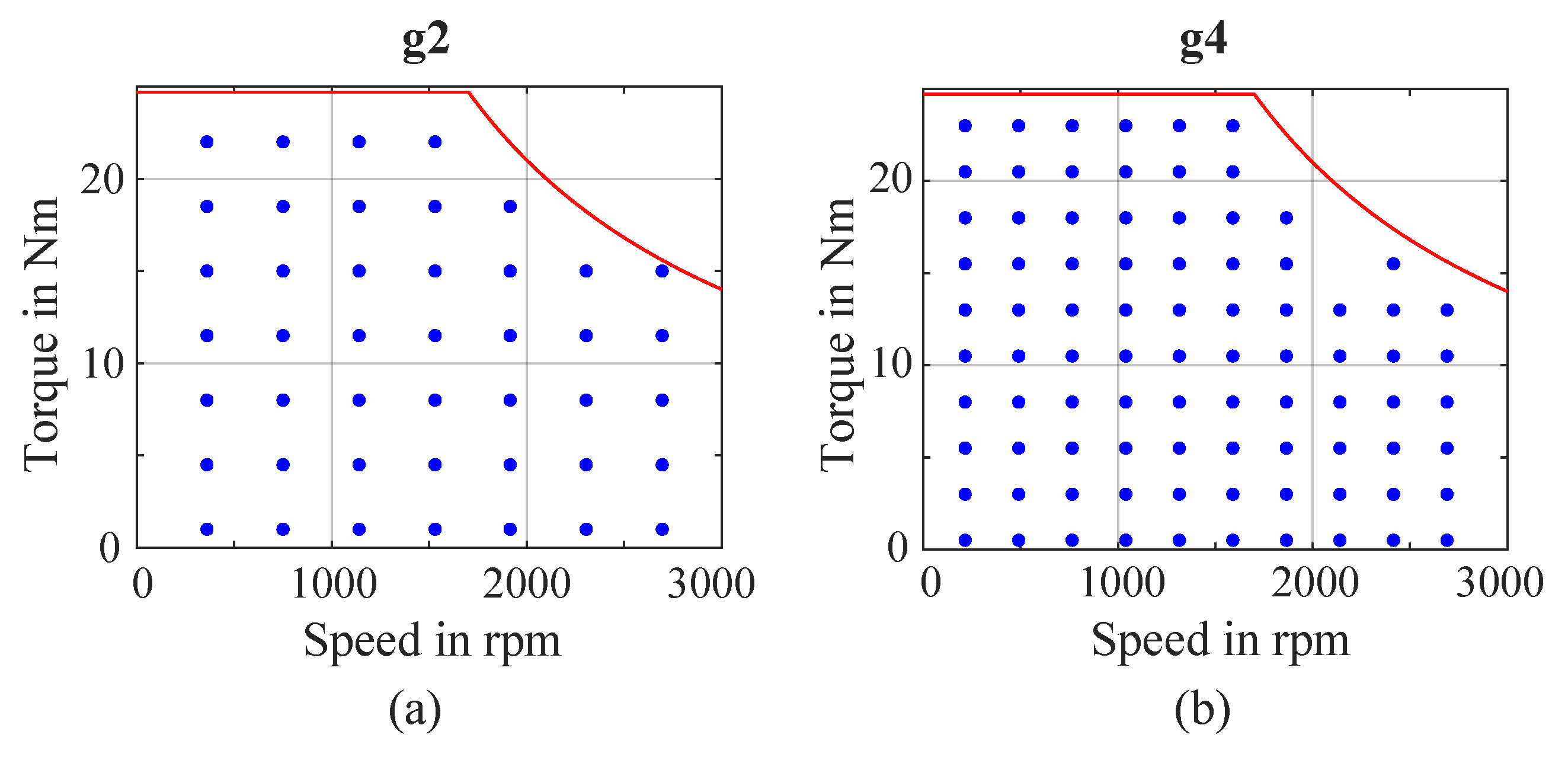
In total, six sets of drive cycle OPs (three cycles across two vehicles) are prepared for evaluation. For the time-stepping method, these OPs are directly applied in both analytic simulation and laboratory tests, with experimental data serving as the performance benchmark for the study. In the LUT-based approach, five sets of evenly distributed grid points are defined: 22, 44, 66, 88, and 113 points (g1-g5). These values refer to the number of grid points in one region (either motoring or generating); therefore, each configuration includes twice the stated number when both regions are considered. The grid points are symmetrically distributed across the motoring and generating regions, spanning a torque range from 0 to 24 Nm and a speed range up to 2700 rpm, in accordance with the test-bench limits. Representative examples of the 22-, 66-, and 113-point configurations (g1, g3, and g5) in the motoring region are shown in Figure 2, while the generating region uses mirrored distributions. The remaining configurations (g2 and g4) are provided in the Figure A1 in Appendix A.
Efficiency at all steady-state grid points is evaluated across five grid resolutions using three methods: an analytic MATLAB model, FEA in JMAG®, and experimental measurements. For each method and resolution, efficiency maps are generated over the defined OPs. To assess drive cycle performance, the down-scaled OPs from the drive cycles are interpolated over these maps, and the resulting efficiency values are compared against direct experimental measurements. The overall workflow of the study is summarized in Figure 3.
2.2. Setting Up the Models
2.2.1. Analytic Model
The analytic analysis was carried out in MATLAB/Simulink [40], where a detailed dynamic model of the IM and its control system was developed, tailored to the constraints of the laboratory test rig. The model integrates an equivalent circuit representation of the IM, operated under Rotor Flux Oriented Control (RFOC), as depicted in Figure 4. This control scheme was chosen for its ability to capture the transient responses needed during drive cycle operation, and key motor parameters, including resistances, inductances, and magnetizing components, were determined through experimental testing. The model also incorporates experimentally derived representations of both iron losses and friction losses, reflecting the physical behavior observed in the laboratory setup. A speed filter and an encoder model are integrated to better replicate the response characteristics of the actual test bench [19]. All measurement data used for model identification are available in [39].
For each torque-speed OP, whether from LUT-based or direct methods, the associated losses are used to calculate the efficiency at that specific condition, as defined in (1). Here, is the output power, represents copper losses, including both stator winding and rotor cage losses, denotes iron losses, and accounts for mechanical friction losses. For OPs in the generating region (i.e., negative torque and positive speed), the definitions of input and output power are reversed, and the efficiency is calculated accordingly.
In the LUT-based approach, each predefined torque-speed point is simulated for 30 seconds to reach steady state before proceeding to the next, repeated across five grid resolutions. By contrast, the time-stepping method applies a down-scaled drive cycle continuously to the analytic model, capturing both dynamic behavior and control interactions.
2.2.2. FEA Model
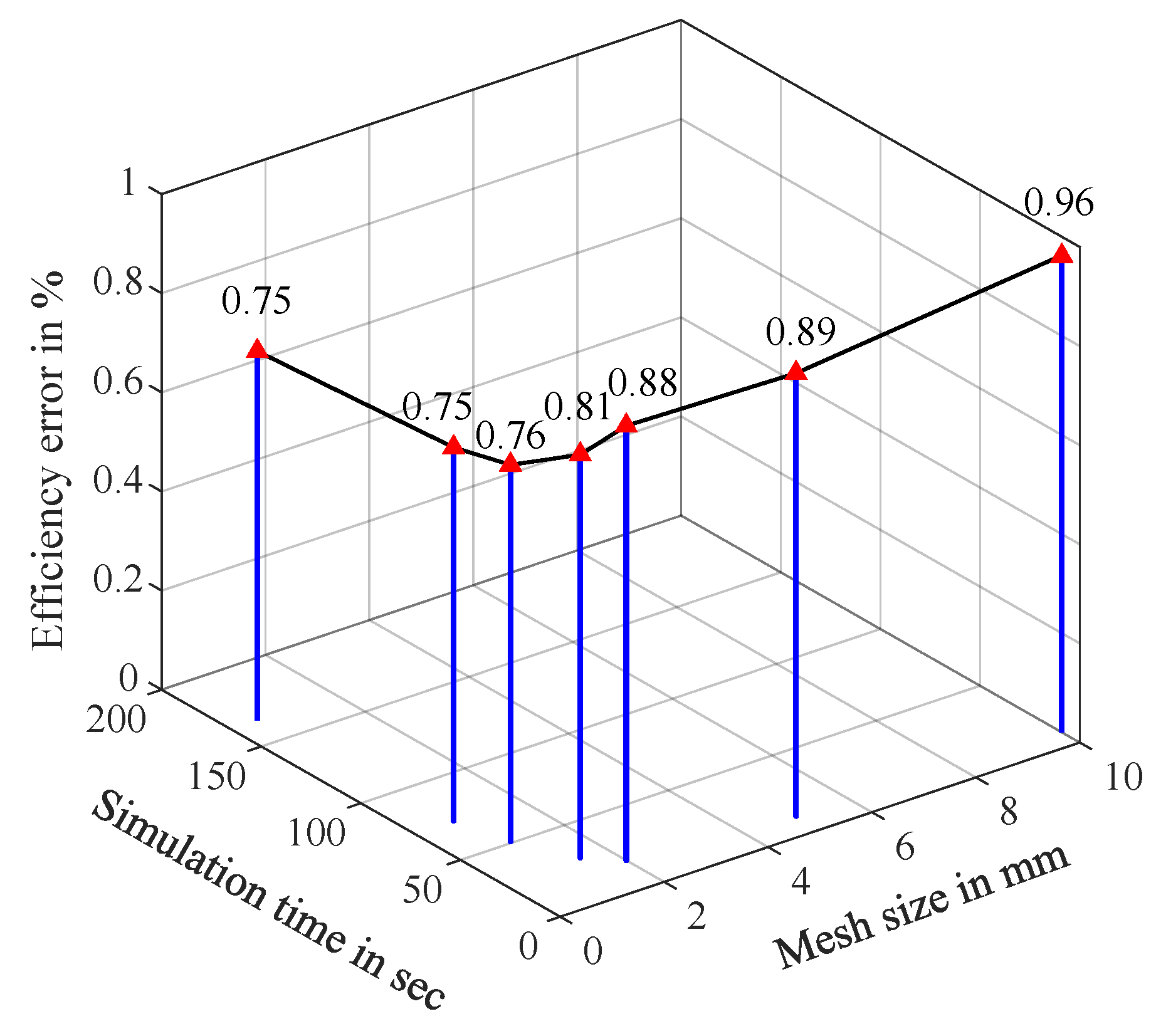
The FEA simulations were performed using the JMAG® software environment [41], which supports high-fidelity analysis of electric machines in both 2D and 3D domains. Although a 3D model was initially tested, it proved too computationally intensive for drive cycle analysis. Therefore, a detailed 2D electromagnetic model was developed for this study, incorporating accurate motor geometry and material properties. The model includes stator iron losses, detailed winding configuration, and rotor-specific parameters such as end-ring leakage inductance and cage resistance. Copper and iron losses are obtained from FEA, while frictional losses are determined experimentally and added post-simulation to complete the efficiency calculation at each OP. A 2D representation of the motor model is shown in Figure 5. To ensure a balance between simulation accuracy and computational efficiency, a mesh resolution of 1 mm was used in all FEA simulations. This mesh size was selected based on a resolution study that evaluated the trade-off between computational time and solution accuracy at a representative OP, as presented in Figure A2 in the Appendix B.
Due to software limitations in directly implementing complex control algorithms, the required control inputs were determined externally using an analytic RFOC model. The stator current magnitude, frequency, and motor slip from the analytic model were then used to define the inputs of the three-phase current source supplying the motor within the software circuit to achieve the desired torque-speed operating points. Each grid point was simulated for two electrical cycles after reaching steady state to ensure that the computed losses and efficiency values accurately reflect stable electromagnetic behavior.
2.3. Test Bench Setup and Configuration
To analyze the down-scaled drive cycles and LUT-based OPs, a dedicated laboratory setup was employed. The configuration of the system is illustrated in the schematic diagram in Figure 6. It consists of the IM as the device under test (DUT), operated under RFOC and mechanically coupled to a torque-controlled PMSM acting as the load machine. The test bench is shown in Figure 7. During each test, key electrical and mechanical parameters including stator voltage, stator current, output torque, and rotor speed were continuously measured. These measurements were used to compute the input and output power, from which the motor efficiency was calculated for each OP. For the LUT-based efficiency mapping, each OP was tested for 30 seconds to ensure waveform stability and accurate energy calculation. For the time-stepping measurements of the down-scaled drive cycles based on the BMW i3 and Smart EQ motors, OPs were evaluated using time steps of 1.14 s and 0.97 s, respectively, according to the applied down-scaling method.
3. Results of Analysis
In this section, the results of both the LUT-based methods and the direct time-stepping approaches are presented. For each OP, whether obtained from measurement or simulation, input and output energies were first calculated, followed by the determination of input and output powers. Using the direction of power flow and the performance definition provided in (1), the efficiency at each OP was then computed. In the generating mode, if the measured losses exceeded the mechanical power, the efficiency could not be reliably defined. To ensure consistency across the dataset, the efficiency for such OPs was conservatively set to zero in this study.
3.1. Steady-State Efficiency Map Analysis
All efficiency maps for the LUT-based approach were generated across five grid resolutions using all three techniques. As an example, Figure 8 presents the efficiency maps from all methods for two grid configurations: g1 with 22×2 points representing low density, and g5 with 113×2 points representing high density. Efficiency values corresponding to the down-scaled drive cycle OPs were extracted from these maps using MATLAB’s default linear interpolation method. As a representative case, Figure 9 presents the efficiency plots for the down-scaled WLTP drive cycle (based on the BMW i3), comparing two grid resolutions and all LUT-based methods.
3.2. Direct Time-stepping Analysis
3.2.1. Analytic Model
The analytic time-stepping method was applied to all down-scaled drive cycles, where each OP was simulated under room temperature conditions to reflect standard laboratory operating environments. This approach enabled the dynamic evaluation of the motor’s performance across time-varying torque-speed profiles, capturing transient effects that are not represented in steady-state methods. As an illustrative example, Figure 10(a) presents the resulting efficiency plot for the down-scaled WLTP drive cycle OPs derived from the BMW i3 motor.
3.2.2. Experimental Direct Method (Baseline Measurement)
The experimental time-stepping analysis was used as the baseline reference to validate both the LUT-based methods and the direct analytic simulation. The IM was tested under all six down-scaled drive cycles corresponding to both vehicle motors. As a representative case in this study, Figure 10(b) shows the measured efficiency plot of the IM OPs across the down-scaled WLTP drive cycle (based on the BMW i3). As illustrative baseline measurements for the remaining drive cycle categories, the experimental efficiency plots for the down-scaled Artemis and BCDC drive cycles (both based on the BMW i3) are shown in Figure 11(a) and Figure 11(b), respectively.
4. Discussions of Results
This section presents a comprehensive evaluation of drive cycle performance using both LUT-based methods and the time-stepping analytic model, including total drive cycle electrical energy conversion efficiency, energy loss analysis, and drive cycle OP efficiency accuracy.
4.1. Energy Conversion and Loss Analysis
4.1.1. Computation Method
The energy conversion efficiency of the drive cycle, denoted , quantifies how effectively the motor converts input electrical energy into output mechanical energy. It is defined as the ratio of total output energy to total input energy, as given in (2).
To compute this efficiency over a given drive cycle, both the input and output energies are obtained by summing the product of instantaneous power and the corresponding time step across the entire cycle. These relationships are given by (3) and ():
Here, and represent the input and output power at the i-th time step, respectively, and is the uniform sampling interval. For the down-scaled drive cycles considered in this analysis, the sampling interval is for the profiles derived from the BMW i3, and for those derived from the Smart EQ. The total number of samples, denoted by N, corresponds to the number of discrete time steps spanning the duration of each respective drive cycle.
4.1.2. Results and Discussion
The experimentally obtained reference values for the down-scaled drive cycles, including input energy (), output energy (), and energy conversion efficiency (), are summarized in Table 2. The efficiencies estimated using the three LUT-based approaches across five grid resolutions are summarized in Table 3. Figure 12 further presents the corresponding total energy losses () for the BMW i3-based cycles, offering a clearer view of discrepancies between LUT-based predictions and laboratory measurements.
No single method consistently outperforms the others across all drive cycles. However, analytic and FEA-based LUT methods provide closer estimates at moderate to high grid densities (e.g., g3–g5), with analytic grid g3 showing near alignment with the benchmark. In contrast, the experimental LUT method tends to overestimate efficiency, particularly in high-speed cycles such as WLTP and Artemis, likely due to instability in frictional torque measurements. These deviations are further influenced by interpolation quality and simplified loss modeling. Since LUT-based approaches rely on steady-state efficiency maps, they inherently struggle to capture transient dynamics such as acceleration and deceleration, which limits their predictive accuracy under real-world drive cycle conditions.
Complementary results obtained from the time-stepping analytic method are presented in Table 4. This method calculates losses point-by-point using an analytical formulation across the full drive cycle, directly incorporating dynamic motor behavior and eliminating reliance on interpolated maps. Among all evaluated methods, it shows the best overall alignment with the experimental benchmark, as it accounts for instantaneous variations in input conditions and captures transient load effects.
Finally, it is important to note that the overall energy conversion efficiencies observed across all drive cycles are relatively low compared to typical production-grade EV traction motors. This is expected, as the IM used in this study was not designed for automotive applications but was instead employed as a laboratory test machine for down-scaled cycle replication. As shown in Figure 8 and Figure 9, many drive cycle OPs fall within low-efficiency regions of the motor’s map. Therefore, the modest energy conversion results reflect the design limitations of the test motor rather than deficiencies in the modeling or measurement approach.
4.2. Error Analysis of Drive Cycle OPs Efficiency
4.2.1. Evaluation Method
To evaluate the accuracy of drive cycle performance predictions and quantify method-related deviations from time-stepping experimental results, two common statistical error metrics are typically employed—Mean Absolute Error (MAE) and Root Mean Square Error (RMSE). RMSE penalizes larger errors more heavily and is appropriate when the error distribution is approximately normal. In contrast, MAE assigns equal weight to all errors and is more robust to outliers, making it more suitable for Laplacian error distributions. Analysis indicates that the distribution of OP efficiencies within the drive cycles follows a Laplace distribution. Therefore, MAE was selected as the primary evaluation metric in this study. MAE is calculated using (5), where n is the total number of data points, is the corresponding efficiency obtained from time-stepping measurements, and represents the efficiency value predicted by the respective method [42,43].
4.2.2. LUT-Based Method Analysis
Table 5 presents the error analysis of various LUT-based methods at different grid resolutions compared to measurements across all down-scaled drive cycles. To further illustrate the trend, Figure 13 further illustrates the MAE for three down-scaled WLTP cycles (based on the BMW i3) across all methods and five grid distributions. In general, MAE decreases as the number of grid points increases, indicating improved accuracy with finer grids. However, increasing evenly distributed points does not always reduce error; for example, grid g3 (66×2) shows lower MAE than grid g4 (88×2) in some cases. This is likely due to interpolation issues and the spatial arrangement of points, where poor placement can cause extrapolation or distortion in regions with concentrated OPs. Based on the selected drive cycles in this study and assuming evenly distributed grid points, this suggests the existence of an optimal grid density, beyond which increasing the number of grid points does not necessarily reduce the error and may even increase it due to local interpolation artifacts.
To highlight the effect of grid resolution on efficiency prediction, Figure 14 compares efficiency differences for the down-scaled WLTP drive cycle (based on the BMW i3) using experimental LUT-based grids g1 and g5. Grid g1 shows larger errors, particularly in the low-speed, low-torque region due to sparse OP coverage. Deviations also appear in the negative-torque region, linked to interpolation or efficiency definition under regeneration. The high-speed Artemis cycle exhibits greater errors than BCDC, mainly from unstable friction torque in the test rig affecting both measurements and loss modeling.
Additionally, When comparing different methods using the same grid points, the FEA-based approach generally yields lower errors than the analytic method. The experimental method, however, exhibits higher errors than both approaches, mainly due to discrepancies between the reference and measured OPs. These mismatches, shown in Figure 15 for grids g4 and g5 as examples, lead to deviations in the efficiency maps, particularly visible for grid g5, as illustrated in Figure 16. On average, the maps deviate by about 3%, with errors concentrated in the low-torque region, which is particularly sensitive to interpolation inaccuracies. Furthermore, the MAE between the reference and measured OPs amounts to 0.51 Nm for grid g4 and 0.47 Nm for grid g5, underscoring the alignment challenges inherent in experimental measurements.
4.2.3. Time-Stepping Analytic Method Analysis
In the direct analytic approach, the MAE is consistently lower than in LUT-based methods across all six down-scaled drive cycles, as shown in Table 4. This is due to detailed modeling of major loss components and the ability to capture transient behaviors such as acceleration and deceleration.
Despite its higher accuracy, discrepancies with experimental results remain, mainly from friction loss modeling errors at high speeds and differences in the field weakening transition. In experiments, this transition is affected by inverter constraints, whereas in the model it follows the motor’s torque-speed profile, causing mismatches in current and losses.
5. Sensitivity of Efficiency Maps to Grid Placement and Temperature
This section analyzes how the accuracy of efficiency maps is influenced by grid point distribution and motor temperature, which are two critical factors affecting drive cycle performance predictions.
5.1. Different Grid Distributions effect on Efficiency Maps
To assess the impact of torque-speed point placement on interpolation error, six grid variations with the same density as g5 (113 points) were analyzed. The torque-speed points span from 0.5 to 24.7 Nm and 100 to 2700 rpm, and their performance was evaluated using analytic simulations. Efficiency maps were generated for each configuration, and drive cycle OPs were extracted from down-scaled drive cycles (based on the BMW i3). As illustrated in Figure 17, the six grid points are defined as follows: Grid 1 (A) features fine torque steps and coarse speed steps; Grid 2 (B) includes fine speed points and coarse torque points; Grid 3 (C) employs quadratic spacing in torque and uniform spacing in speed; Grid 4 (D) applies uniform spacing in torque and quadratic spacing in speed; Grid 5 (E) corresponds to the baseline configuration used in this study (g5); and Grid 6 (F) utilizes quadratic spacing in both torque and speed directions.
As shown in the error analysis of different grids for the energy conversion efficiency of the complete drive cycles and the MAE of the drive cycle OPs in Figure 17, grid B exhibits the highest overall error, including the largest deviations in both total energy efficiency and the efficiency of drive cycle OPs. This is primarily due to the coarse resolution in the torque direction, which leads to extensive interpolation and thus reduced accuracy in the generated efficiency maps. Overall, the analysis highlights that even with a relatively high number of grid points, the accuracy of efficiency maps is highly dependent on the spatial distribution of those points. Therefore, careful placement of grid points in the torque-speed plane is essential for constructing reliable and precise efficiency maps.
5.2. Effect of Temperature on Efficiency Map Accuracy
To enhance the accuracy of efficiency map analysis, the thermal condition of the motor must be considered. An increase in temperature, particularly in the windings, raises copper losses and alters the motor’s overall efficiency, thereby affecting the accuracy of drive cycle predictions. Figure 18 presents analytically derived efficiency maps at 20,°C and 100,°C. As shown, the 85% efficiency contour visible at 20°C disappears at 100 °C, indicating a significant loss in efficiency at elevated temperatures. This demonstrates that temperature has a considerable impact on efficiency prediction and highlights the importance of evaluating or correcting efficiency maps based on the thermal conditions under which drive cycles are measured.
6. Analysis of Accuracy Factors and Computational Efficiency
6.1. Factors Influencing Performance Prediction Accuracy of the Methods
The accuracy of efficiency prediction for the IM during drive cycle operation is influenced by several factors. In LUT-based methods, errors mainly arise from interpolation inaccuracies and mismatches between simulated reference and measured torque-speed OPs, as discussed earlier. Other factors affecting both LUT-based and time-stepping methods include friction and mechanical losses, which vary with speed, temperature, and test duration, as well as simplified loss modeling that neglects effects such as magnetic saturation, harmonic losses, and PWM influences. Control-related errors are minimal since both methods use the same RFOC strategy. The choice of mesh resolution also impacts simulation accuracy; as shown in Figure A2 in the Appendix B, increasing the mesh density beyond a certain threshold provides only marginal improvements, indicating a trade-off between computational cost and accuracy.
Temperature effects play an important role in performance prediction. Figure 19 shows the temperature evolution of all main motor components during a down-scaled WLTP drive cycle based on the BMW i3. Key loss-contributing components, such as the stator windings and rotor, exhibited temperature increases of 7–12°C. While these changes are modest, they can still influence copper resistance and iron losses, highlighting the importance of incorporating thermal effects into performance modeling. Table 6 provides a qualitative summary of the main factors affecting efficiency prediction accuracy for both LUT-based and time-stepping methods.
6.2. Computational Efficiency of Methods
Computational efficiency is critical for selecting a method to evaluate drive cycle performance in EV motor design. Table 7 shows simulation times for direct analytic and LUT-based methods across different grids. LUT-based methods require extra post-processing to extract OP efficiencies, increasing total time. The direct analytic method is the fastest, relying on predefined loss models, though accurate results require careful calibration of key parameters such as friction and iron losses.
The FEA-based LUT method is the most computationally demanding due to the detailed field solution at each grid point. Similarly, the experimental LUT method involves long test-bench durations that scale with grid density. In contrast, the analytic LUT-based approach offers a good balance between accuracy and simulation time. For instance, grid g5 requires only 38 seconds to complete the full map while still delivering reasonable agreement with time-stepping results, provided that the grid is designed with attention to drive cycle OP distribution. This emphasizes the importance of grid placement, as the accuracy of LUT-based predictions strongly depends not just on the number of points but also on where those points lie in the torque-speed plane.
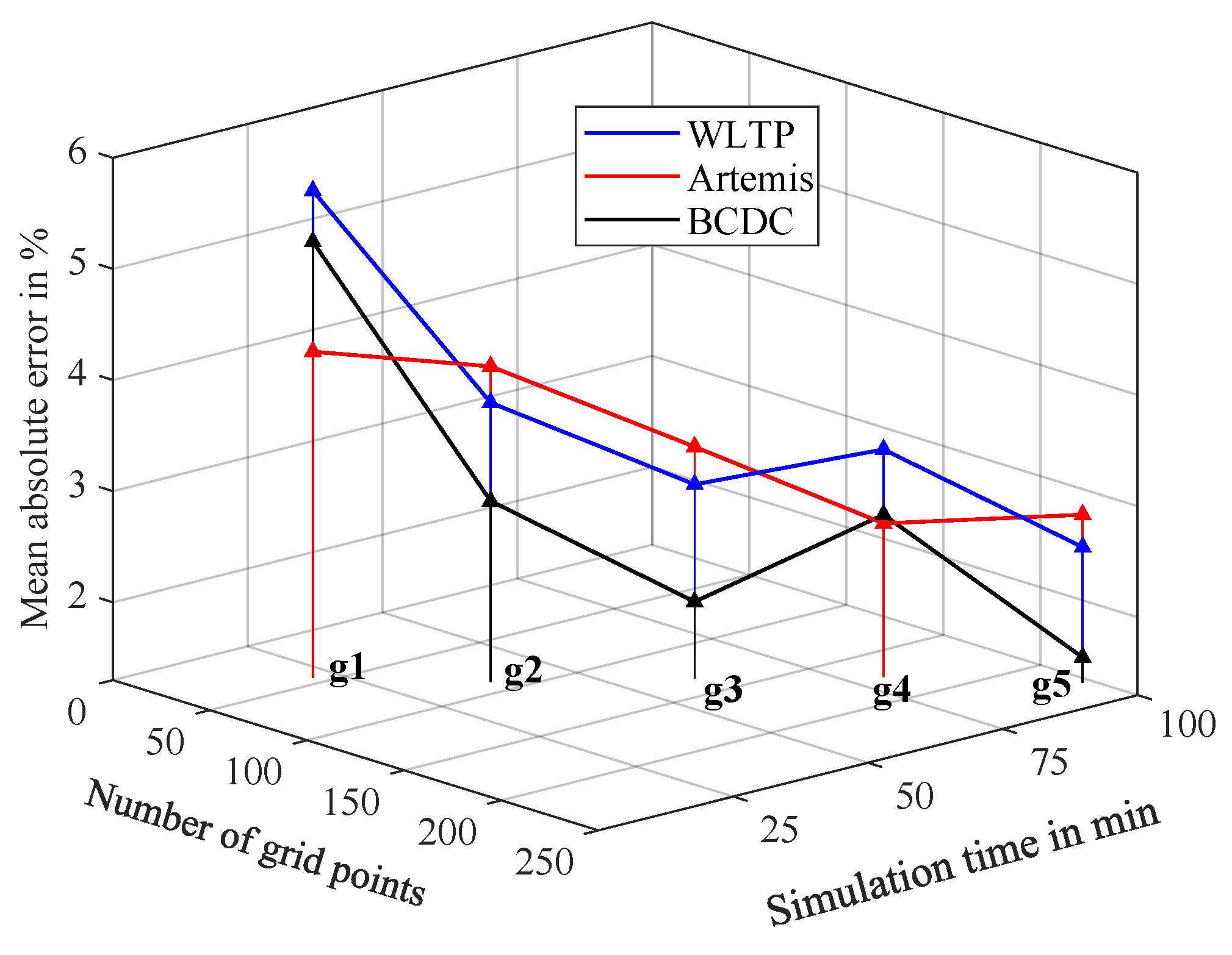
Figure 20 shows the trade-off between grid density, simulation time, and MAE for the BMW i3–based cycles using FEA. Increasing grid points generally reduces MAE but at higher cost, with optimized grid placement achieving low errors with fewer simulations. Overall, carefully designed LUT-based maps can closely match time-stepping measurements while maintaining low computational effort.
7. Conclusions
This study presents a comprehensive evaluation of three LUT-based methods and one time-stepping simulation approach for assessing the performance of a laboratory-scale IM under dynamic drive cycles. By comparing all methods with experimental time-stepping measurements across three standard drive cycles and two EV platforms, the research quantifies overall energy efficiency deviations as well as point-wise accuracy across different grid resolutions and modeling techniques.
Results showed that while LUT-based methods are computationally efficient and widely used in EV simulations, their predictive accuracy strongly depends on the number and distribution of grid points. Poorly placed or coarse grids can introduce significant interpolation errors, particularly in regions with dense drive cycle OPs. In contrast, time-stepping simulations provide more accurate results by capturing transient dynamics and loss mechanisms, although they rely on experimentally derived loss parameters for accuracy.
A sensitivity analysis demonstrated that both grid distribution and temperature variation significantly affect the accuracy of efficiency maps. Non-uniform grids, especially those with insufficient resolution in the torque direction, can degrade performance prediction. Similarly, neglecting thermal effects leads to overestimated efficiency, highlighting the importance of temperature-aware mapping for reliable evaluation.
Among all methods, the direct analytic time-stepping approach demonstrated the closest overall agreement with experimental data. However, analytically derived LUTs, when paired with well-designed grid configurations tailored to the target drive cycle OPs, offered a favorable trade-off between computational efficiency and accuracy, making them well-suited for design and optimization workflows.
Author Contributions
Conceptualization, K.H., P.K.D. and A.M.; Measurements, K.H. and R.S.; Investigation and validation, K.H. and P.K.D; Writing—original draft, K.H.; Supervision, A.M.; All authors have read and agreed to the published version of the manuscript.
Funding
This work is partially supported by the joint Collaborative Research Centre CREATOR (DFG: Project-ID 492661287/TRR 361; FWF: 10.55776/F90) at TU Darmstadt, TU Graz and JKU Linz. For the purpose of open access, the author has applied a CC BY public copyright license to any Author Accepted Manuscript version arising from this submission.
Data Availability Statement
An openly published dataset for the induction machine used in this study is available in [39]. It provides complete design specifications—including electrical, mechanical, geometrical, winding, and material details—along with performance measurements under steady-state and transient drive cycle conditions.
Acknowledgments
ChatGPT-4o [44] was used for language editing and grammar enhancement. The paper was subsequently refined through additional manual editing.
Conflicts of Interest
The authors declare no conflicts of interest.
Appendix A
Figure A1.
Grid configurations for LUT-based analyses: (a) 44×2 points (g2), (b) 88×2 points (g4).
Appendix B
Figure A2.
Effect of mesh resolution on simulation accuracy and computational time for an IM operating point at 11.5 Nm and 1530 rpm, with a measured efficiency of 86.26 %.
Figure A2.
Effect of mesh resolution on simulation accuracy and computational time for an IM operating point at 11.5 Nm and 1530 rpm, with a measured efficiency of 86.26 %.
References
- Heidarikani, K.; Dhakal, P.K.; Seebacher, R.; Muetze, A. Quantification of Steady-State Efficiency Maps and Time-Stepping Solutions for Drive Cycle Performance Analysis of Induction Motors. In Proceedings of the 2024 27th International Conference on Electrical Machines and Systems (ICEMS), Fukuoka, Japan, nov 2024; pp. 1–6. [Google Scholar] [CrossRef]
- Wang, J.; Zhang, C.; Guo, D.; Yang, F.; Zhang, Z.; Zhao, M. Drive-Cycle-Based Configuration Design and Energy Efficiency Analysis of Dual-Motor 4WD System With Two-Speed Transmission for Electric Vehicles. IEEE Transactions on Transportation Electrification 2024, 10, 1887–1899. [Google Scholar] [CrossRef]
- Cheng, Y.; Wang, Y.; Ma, J.; Liu, G.; Li, D.; Qu, R. Fast Evaluation of Driving Cycle Efficiency of Interior Permanent Magnet Synchronous Machines for Electric Vehicles Considering Step-Skewing. IEEE Transactions on Industry Applications 2024, 60, 4396–4407. [Google Scholar] [CrossRef]
- Mariasiu, F. Performance Analysis and Simulation of Electric Vehicles. Energies 2025, 18, 2365. [Google Scholar] [CrossRef]
- Huynh, T.A.; Chen, P.H.; Hsieh, M.F. Analysis and Comparison of Operational Characteristics of Electric Vehicle Traction Units Combining Two Different Types of Motors. IEEE Transactions on Vehicular Technology 2022, 71, 5727–5742. [Google Scholar] [CrossRef]
- Mahmouditabar, F.; Baker, N.J. Design Optimization of Induction Motors with Different Stator Slot Rotor Bar Combinations Considering Drive Cycle. Energies 2024, 17, 154. [Google Scholar] [CrossRef]
- Praslicka, B.; Ma, C.; Taran, N. A Computationally Efficient High-Fidelity Multi-Physics Design Optimization of Traction Motors for Drive Cycle Loss Minimization. IEEE Transactions on Industry Applications 2023, 59, 1351–1360. [Google Scholar] [CrossRef]
- Krishnamoorthy, S.; Panikkar, P.P.K. A comprehensive review of different electric motors for electric vehicles application. IJPEDS 2024, 15, 74. [Google Scholar] [CrossRef]
- Mavlonov, J.; Ruzimov, S.; Tonoli, A.; Amati, N.; Mukhitdinov, A. Sensitivity Analysis of Electric Energy Consumption in Battery Electric Vehicles with Different Electric Motors. World Electric Vehicle Journal 2023, 14. [Google Scholar] [CrossRef]
- Peng, Y.; Chen, F.; Chen, F.; Wu, C.; Wang, Q.; He, Z.; Lu, S. Energy-efficient Train Control: A Comparative Study based on Permanent Magnet Synchronous Motor and Induction Motor. IEEE Transactions on Vehicular Technology 2024, pp. 1–13. [CrossRef]
- Yoo, J.; Lee, J.H.; Sul, S.K. FEA-Assisted Experimental Parameter Map Identification of Induction Motor for Wide-Range Field-Oriented Control. IEEE Trans. Power Electron. 2024, 39, 1353–1363. [Google Scholar] [CrossRef]
- Roshandel, E.; Mahmoudi, A.; Soong, W.L.; Kahourzade, S. Optimal Design of Induction Motors Over Driving Cycles for Electric Vehicles. IEEE Transactions on Vehicular Technology 2023, 72, 15548–15562. [Google Scholar] [CrossRef]
- Roshandel, E.; Mahmoudi, A.; Kahourzade, S.; Soong, W.L. Efficiency Maps of Electrical Machines: A Tutorial Review. IEEE Transactions on Industry Applications 2023, 59, 1263–1272. [Google Scholar] [CrossRef]
- Stiscia, O.; Rubino, S.; Vaschetto, S.; Cavagnino, A.; Tenconi, A. Accurate Induction Machines Efficiency Mapping Computed by Standard Test Parameters. IEEE Transactions on Industry Applications 2022, 58, 3522–3532. [Google Scholar] [CrossRef]
- Lanzara, G. Electric motor test bench for efficiency maps generation. laurea, Politecnico di Torino, 2021.
- Karkkainen, H.; Aarniovuori, L.; Niemela, M.; Pyrhonen, J. Converter-Fed Induction Motor Efficiency: Practical Applicability of IEC Methods. IEEE Industrial Electronics Magazine 2017, 11. [Google Scholar] [CrossRef]
- Sano, H.; Semba, K.; Suzuki, Y.; Yamada, T. Investigation in the accuracy of FEA Based Efficiency Maps for PMSM traction machines. In Proceedings of the 2022 International Conference on Electrical Machines (ICEM), Valencia, Spain; 2022; pp. 2061–2066. [Google Scholar] [CrossRef]
- Ragazzo, P.; Dilevrano, G.; Bojoi, A.; Ferrari, S.; Pellegrino, G. Fast Efficiency Mapping Procedure for PMSM Accounting for the PWM Supply Impact. In Proceedings of the 2024 IEEE International Conference on Industrial Technology (ICIT); 2024; pp. 1–6. [Google Scholar] [CrossRef]
- Heidarikani, K.; Dhakal, P.K.; Seebacher, R.; Muetze, A. Baseline Determination for Drive Cycle Performance Analysis of Induction Motors. In Proceedings of the 2023 IEEE Transportation Electrification Conference and Expo, Asia-Pacific (ITEC Asia-Pacific), Chiang Mai, Thailand, Nov 2023; pp. 1–6. [Google Scholar] [CrossRef]
- Dhakal, P.K.; Heidarikani, K.; Seebacher, R.; Muetze, A. Baseline Determination for Drive Cycle Performance Analysis of Permanent Magnet Synchronous Motors. In Proceedings of the 2023 IEEE Transportation Electrification Conference and Expo, Asia-Pacific (ITEC Asia-Pacific), Chiang Mai, Thailand, nov 2023; pp. 1–6. [Google Scholar] [CrossRef]
- Pastellides, S.; Gerber, S.; Wang, R.J.; Kamper, M. Evaluation of Drive Cycle-Based Traction Motor Design Strategies Using Gradient Optimisation. Energies 2022, 15, 1095. [Google Scholar] [CrossRef]
- Hwang, S.W.; Ryu, J.Y.; Chin, J.W.; Park, S.H.; Kim, D.K.; Lim, M.S. Coupled Electromagnetic-Thermal Analysis for Predicting Traction Motor Characteristics According to Electric Vehicle Driving Cycle. IEEE Transactions on Vehicular Technology 2021, 70, 4262–4272. [Google Scholar] [CrossRef]
- Mısır, O.; Akar, M. Efficiency and Core Loss Map Estimation with Machine Learning Based Multivariate Polynomial Regression Model. Mathematics 2022, 10, 3691. [Google Scholar] [CrossRef]
- Oyamada, M.; Kunimatsu, S.; Mizumoto, I. Performance Prediction of Electric Motors via Deep Learning. IEEJ Journal IA 2023, 12, 238–243. [Google Scholar] [CrossRef]
- Gong, Y.; Gneiting, A.; Weigel, S.; Parspour, N.; An, Z. Surrogate Model Based Drive Cycle Modelling and Optimization of Synchronous Reluctance Machines for Electric Vehicles. IEEE Transactions on Magnetics 2025, pp. 1–1. [CrossRef]
- Carbonieri, M.; Leonardo, L.D.; Bianchi, N.; Tursini, M.; Villani, M.A.; Popescu, M. Cage Losses in Induction Motors Considering Harmonics: A New Finite Element Procedure and Comparison With the Time-Domain Approach. IEEE Transactions on Industry Applications 2022, 58, 1931–1940. [Google Scholar] [CrossRef]
- Dhakal, P.K.; Heidarikani, K.; Seebacher, R.; Muetze, A. Efficiency Map Versus Time-Stepping Solutions for Drive Cycle Performance Analysis of Permanent Magnet Synchronous Motors. In Proceedings of the 2024 27th International Conference on Electrical Machines and Systems (ICEMS), Fukuoka, Japan, nov 2024; pp. 1–6. [Google Scholar] [CrossRef]
- Fan, D.; Zhu, X.; Quan, L.; Han, P.; Xiang, Z.; Wu, J. Driving Cycle Design Optimization of Less-Rare-Earth PM Motor Using Dimension Reduction Method. IEEE Trans. Energy Convers. 2023, 38, 1614–1625. [Google Scholar] [CrossRef]
- Ruuskanen, V.; Nerg, J.; Pyrhönen, J.; Ruotsalainen, S.; Kennel, R. Drive Cycle Analysis of a Permanent-Magnet Traction Motor Based on Magnetostatic Finite-Element Analysis. IEEE Transactions on Vehicular Technology 2015, 64, 1249–1254. [Google Scholar] [CrossRef]
- Malarselvam, V.; Carunaiselvane, C. Energy Efficient Analysis of Electric Vehicle Motor under Drive Cycle Influence. In Proceedings of the 2023 IEEE International Conference on Power Electronics, Smart Grid, and Renewable Energy (PESGRE), 2023, pp. 1–6. [CrossRef]
- Lacock, S.; du Plessis, A.A.; Booysen, M.J. Electric Vehicle Drivetrain Efficiency and the Multi-Speed Transmission Question. World Electric Vehicle Journal 2023, 14, 342. [Google Scholar] [CrossRef]
- Bhaktha, B.S.; Jose, N.; Vamshik, M.; Pitchaimani, J.; Gangadharan, K.V. Driving Cycle-Based Design Optimization and Experimental Verification of a Switched Reluctance Motor for an E-Rickshaw. IEEE Transactions on Transportation Electrification 2024, 10, 9959–9974. [Google Scholar] [CrossRef]
- Islam, M.S.; Safayet, A.; Islam, M. A Fast Computation Method to Calculate Performances of an Electric Propulsion System for Drive Cycles. In Proceedings of the 2024 IEEE Energy Conversion Congress and Exposition (ECCE), 2024, pp. 2308–2314. ISSN: 2329-3748. [CrossRef]
- DieselNet. Emission Test Cycles. Available online: https://dieselnet.com/standards/cycles/index.php (accessed on 18 August 2025).
- Petersheim, M.D.; Brennan, S.N. Scaling of hybrid-electric vehicle powertrain components for Hardware-in-the-loop simulation. Mechatronics 2009, 19, 1078–1090. [Google Scholar] [CrossRef]
- Dhakal, P.K.; Heidarikani, K.; Muetze, A. Down-scaling of drive cycles for experimental drive cycle analyses. In Proceedings of the 12th International Conference on Power Electronics, Machines and Drives (PEMD 2023), Brussels, Belgium, 2023; Vol. 2023; pp. 271–276. [Google Scholar] [CrossRef]
- BMW Group. Technical Data BMW i3 (120Ah). Available online: https://www.press.bmwgroup.com/global/article/detail/T0148284EN/the-bmw-i3?language=en (accessed on 1 September 2025).
- Smart. Smart EQ fortwo coupe. Available online: https://ev-database.org/car/1230/Smart-EQ-fortwo-coupe (accessed on 1 September 2025).
- Heidarikani, K.; Dhakal, P.K.; Muetze, A.; Seebacher, R. CREATOR Case: Induction Motor Data, 2024. Version Number: 1. [CrossRef]
- MathWorks. MATLAB. Available online: https://www.Mathworks.com/products/matlab.html (accessed on 10 September 2025).
- JSOL. Simulation Technology for Electromechanical Design : JMAG. Available online: https://www.jmag-international.com/ (accessed on 16 September 2025).
- Hodson, T.O. Root-mean-square error (RMSE) or mean absolute error (MAE): When to use them or not. Geoscientific Model Development 2022, 15, 5481–5487. [Google Scholar] [CrossRef]
- Montgomery, D.C.; Peck, E.A.; Vining, G.G. Introduction to Linear Regression Analysis; John Wiley & Sons, 2021.
- OpenAI. ChatGPT-4o. Online; accessed July 29, 2025, 2024. Available online: https://openai.com/chatgpt (accessed on 17 September 2025).
Figure 1.
Standard reference drive cycles: (a) WLTP class 3, (b) Artemis motorway km/hr, (c) Braunschweig city driving cycle [34].
Figure 1.
Standard reference drive cycles: (a) WLTP class 3, (b) Artemis motorway km/hr, (c) Braunschweig city driving cycle [34].
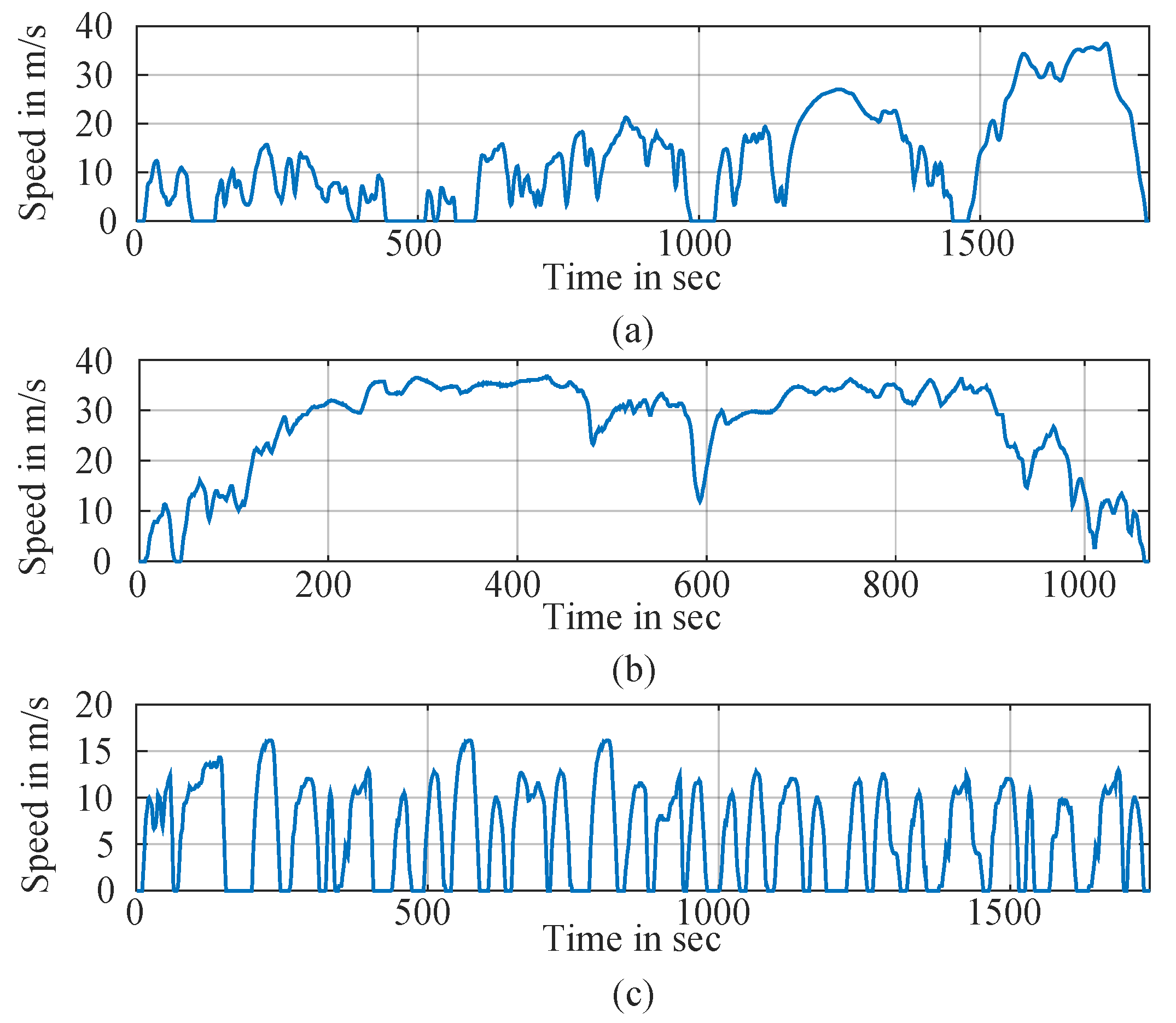
Figure 2.
Grid configurations for LUT-based analyses: (a) 22×2 points (g1), (b) 66×2 points (g3), (c) 113×2 points (g5).
Figure 2.
Grid configurations for LUT-based analyses: (a) 22×2 points (g1), (b) 66×2 points (g3), (c) 113×2 points (g5).
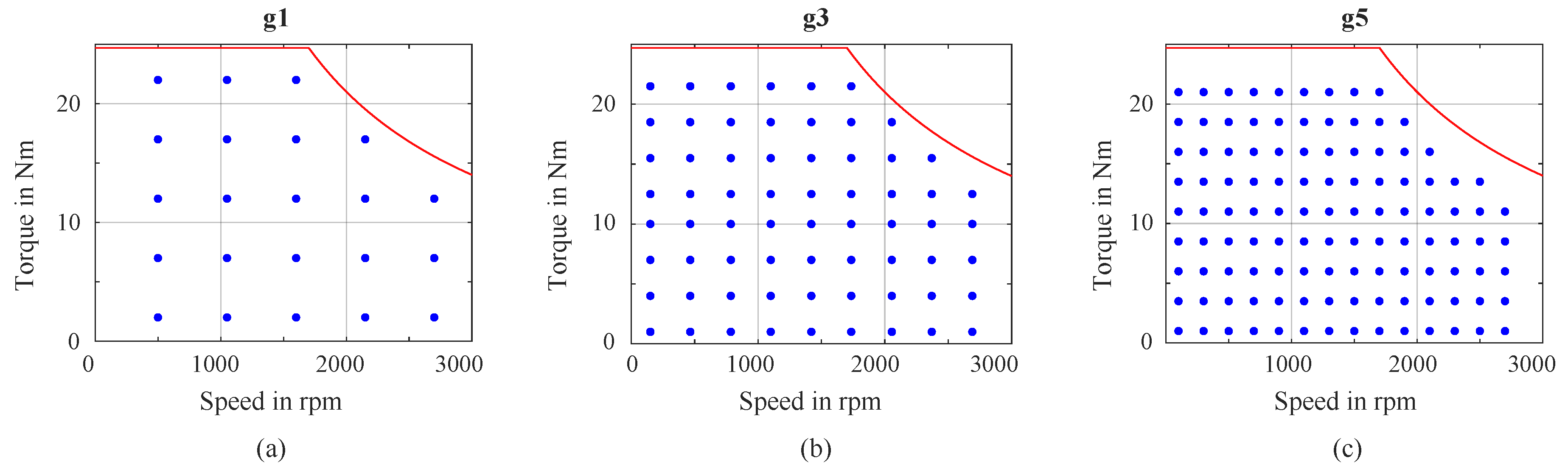
Figure 3.
The flowchart of the study.
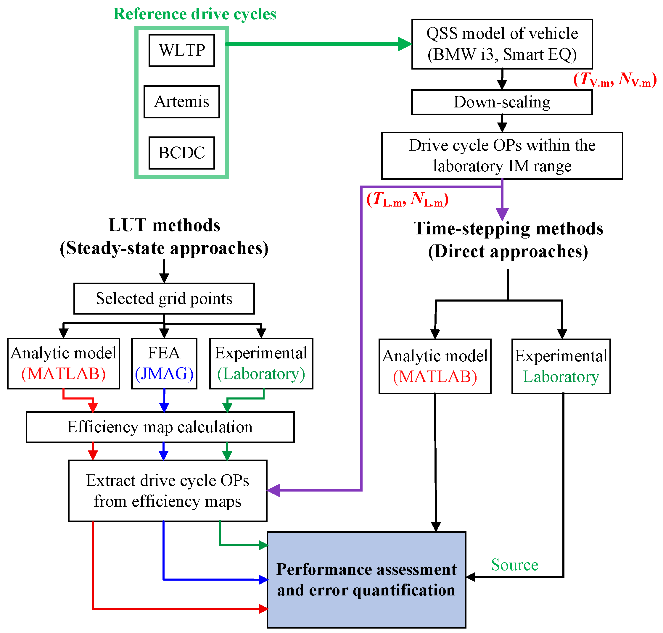
Figure 4.
Control block diagrams depicting the analytic model of the IM.
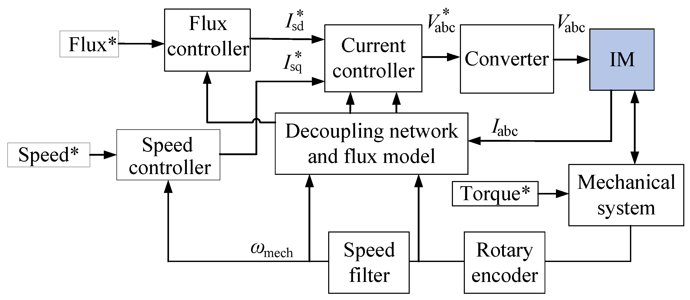
Figure 5.
A 2D FEA model of the laboratory IM in JMAG.
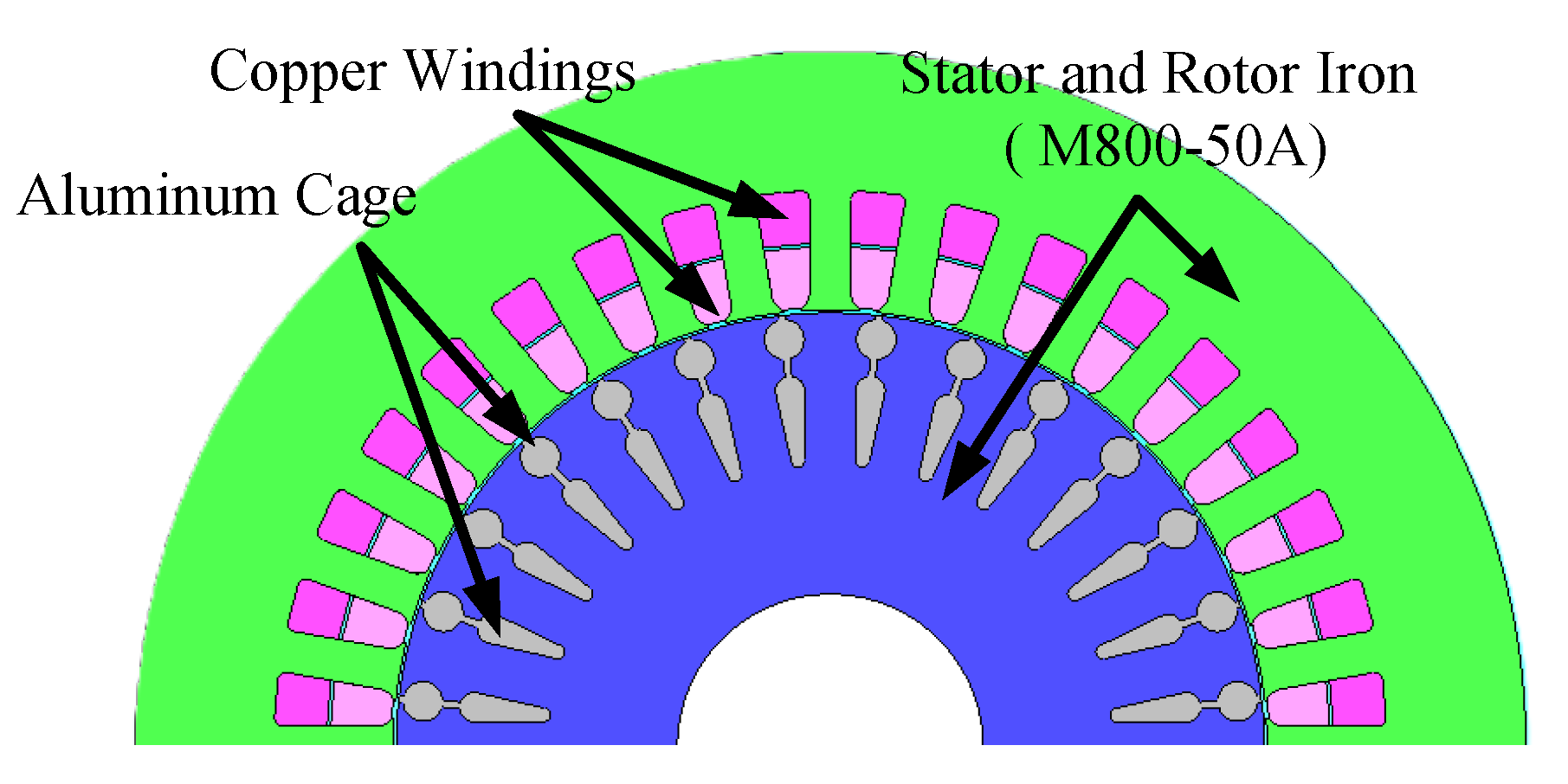
Figure 6.
Schematic diagrams of the laboratory test-bench of the IM.
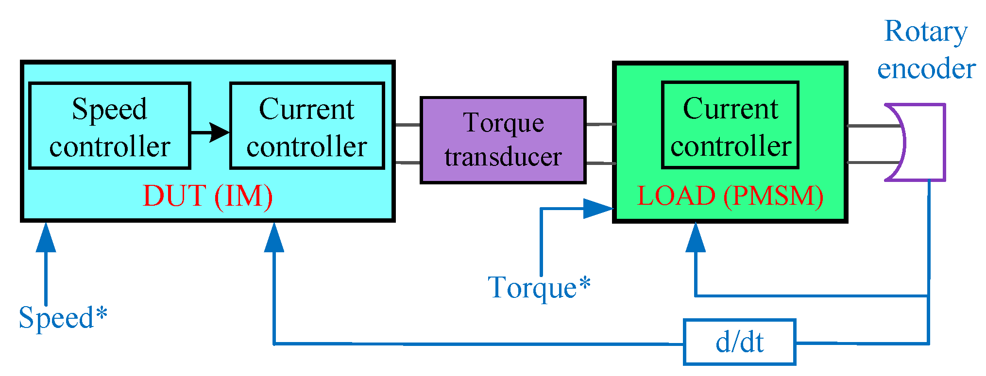
Figure 7.
Laboratory test bench for the IM.
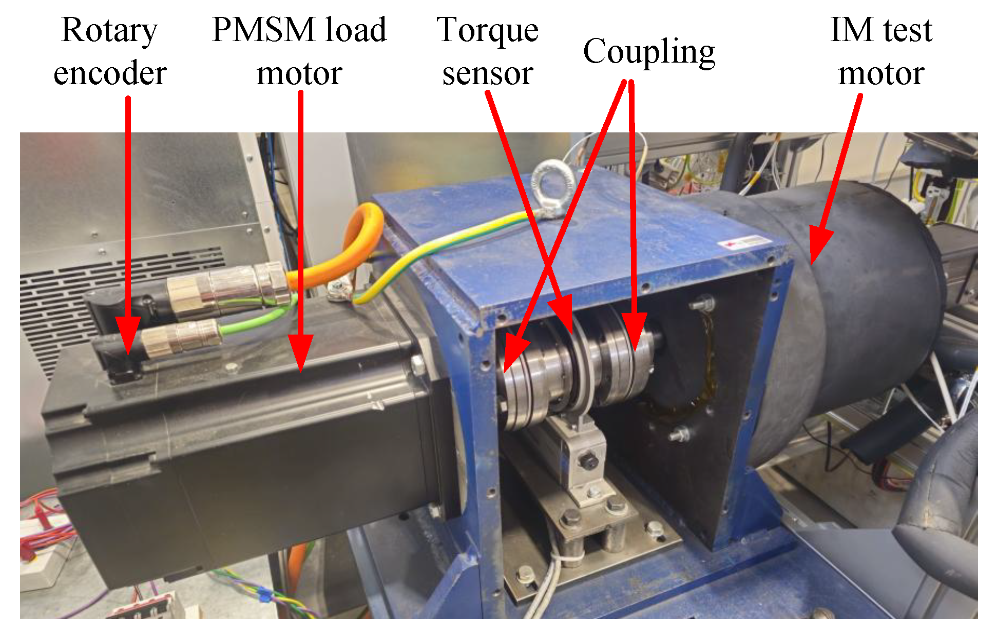
Figure 8.
Efficiency maps computed using various grid point densities and analysis methods.
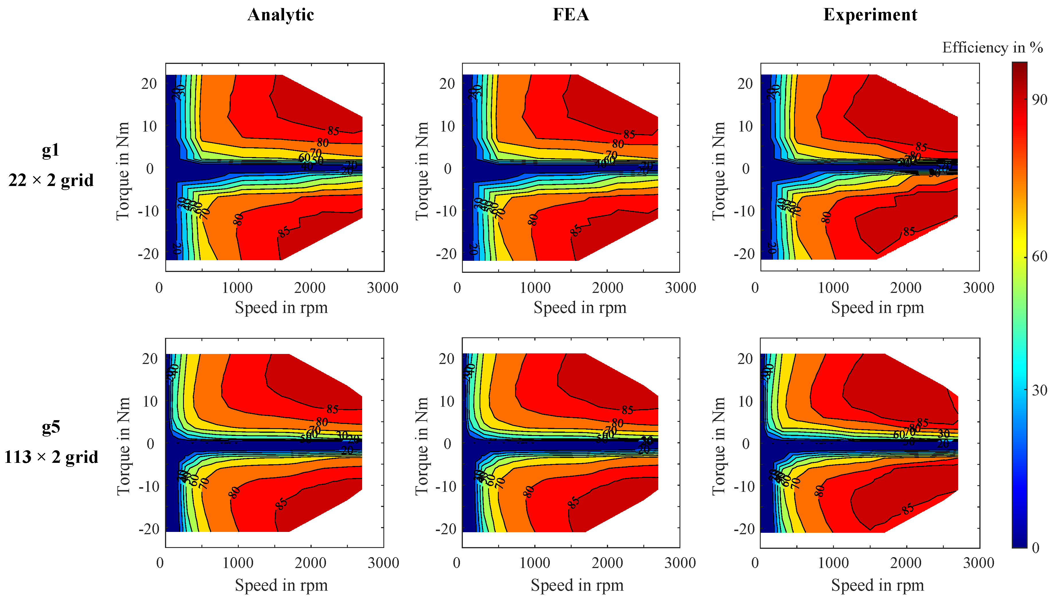
Figure 9.
LUT-based efficiency plots of the IM OPs for the down-scaled WLTP drive cycle (based on the BMW i3), using different grid points and methods.
Figure 9.
LUT-based efficiency plots of the IM OPs for the down-scaled WLTP drive cycle (based on the BMW i3), using different grid points and methods.
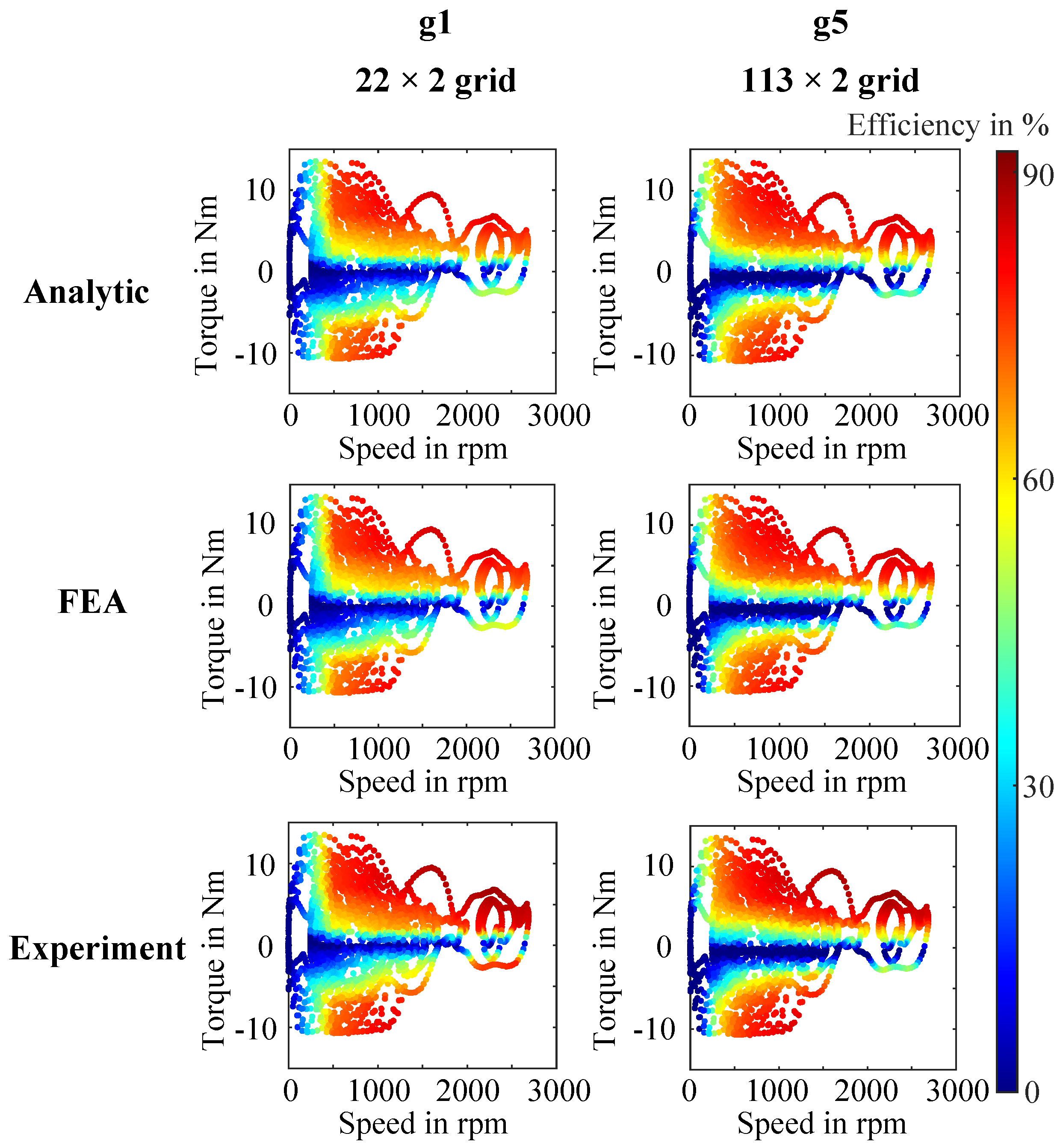
Figure 10.
Efficiency plots of the IM OPs for the down-scaled WLTP drive cycle (based on the BMW i3) using: (a) time-stepping analytic model, and (b) time-stepping measurement.
Figure 10.
Efficiency plots of the IM OPs for the down-scaled WLTP drive cycle (based on the BMW i3) using: (a) time-stepping analytic model, and (b) time-stepping measurement.
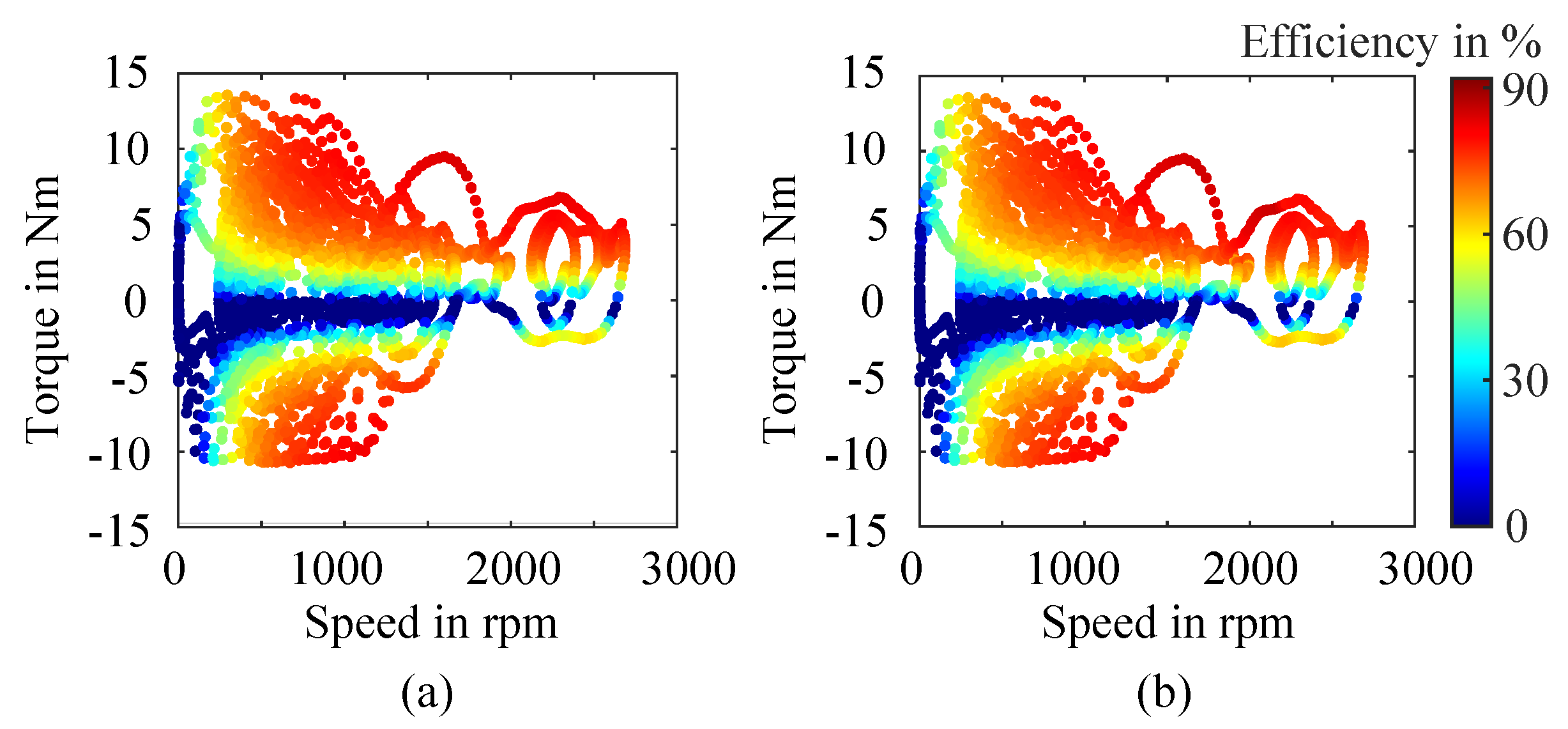
Figure 11.
Efficiency plots of the IM OPs for the down-scaled drive cycles (based on the BMW i3), obtained using time-stepping measurements: (a) Artemis, and (b) BCDC.
Figure 11.
Efficiency plots of the IM OPs for the down-scaled drive cycles (based on the BMW i3), obtained using time-stepping measurements: (a) Artemis, and (b) BCDC.
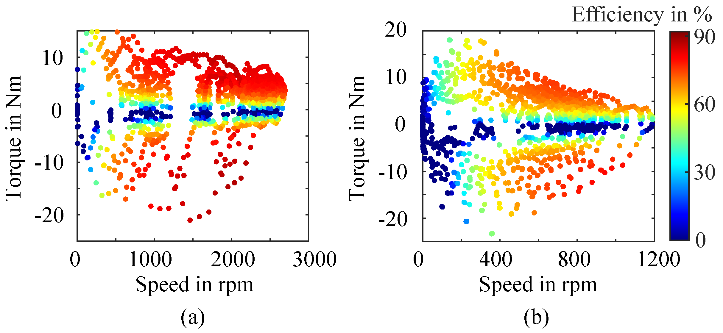
Figure 12.
Loss energy () for each drive cycle ( based on the BMW i3), calculated using LUT-based methods across five grid points and compared against time-stepping laboratory measurements.
Figure 12.
Loss energy () for each drive cycle ( based on the BMW i3), calculated using LUT-based methods across five grid points and compared against time-stepping laboratory measurements.
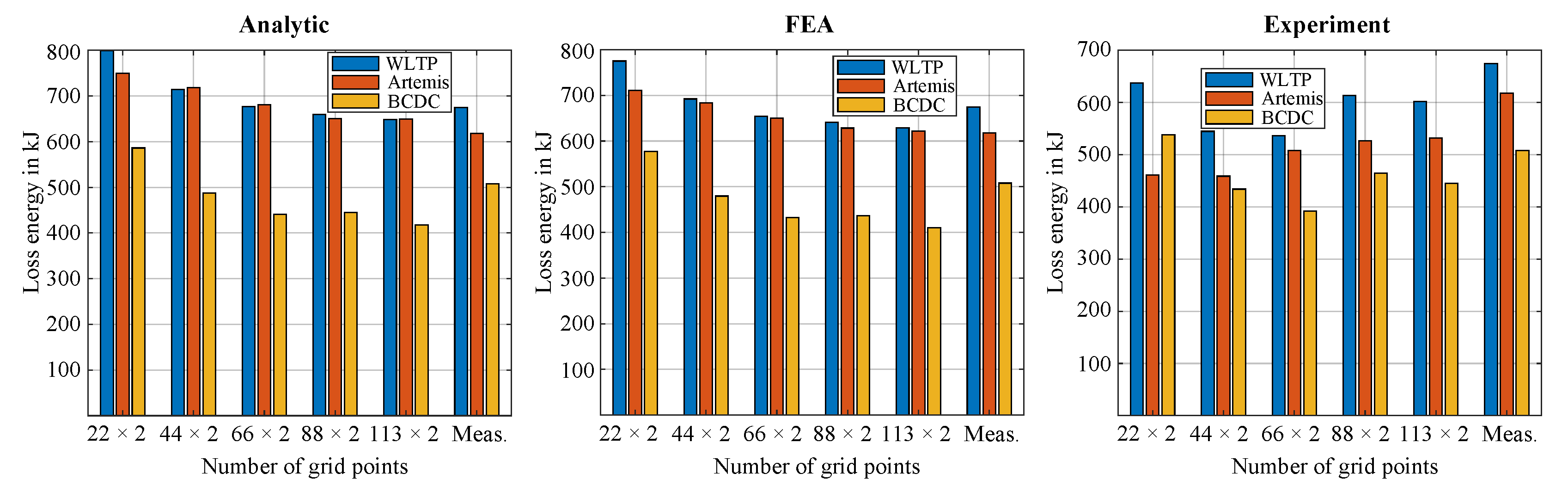
Figure 13.
Mean absolute efficiency error of the IM’s OPs across down-scaled drive cycles (based on the BMW i3), comparing LUT-based methods at various grid points with time-stepping laboratory measurements.
Figure 13.
Mean absolute efficiency error of the IM’s OPs across down-scaled drive cycles (based on the BMW i3), comparing LUT-based methods at various grid points with time-stepping laboratory measurements.
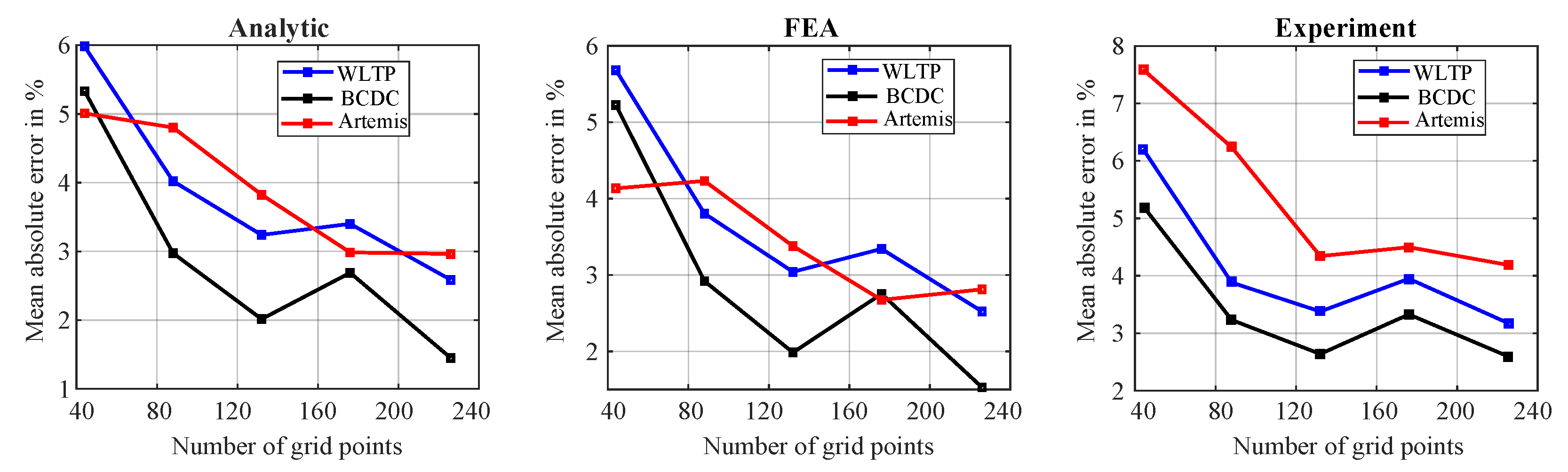
Figure 14.
Absolute efficiency differences between LUT-based and time-stepping measurements for down-scaled WLTP drive cycle OPs (BMW i3) from (a) grid g1 and (b) grid g5..
Figure 14.
Absolute efficiency differences between LUT-based and time-stepping measurements for down-scaled WLTP drive cycle OPs (BMW i3) from (a) grid g1 and (b) grid g5..
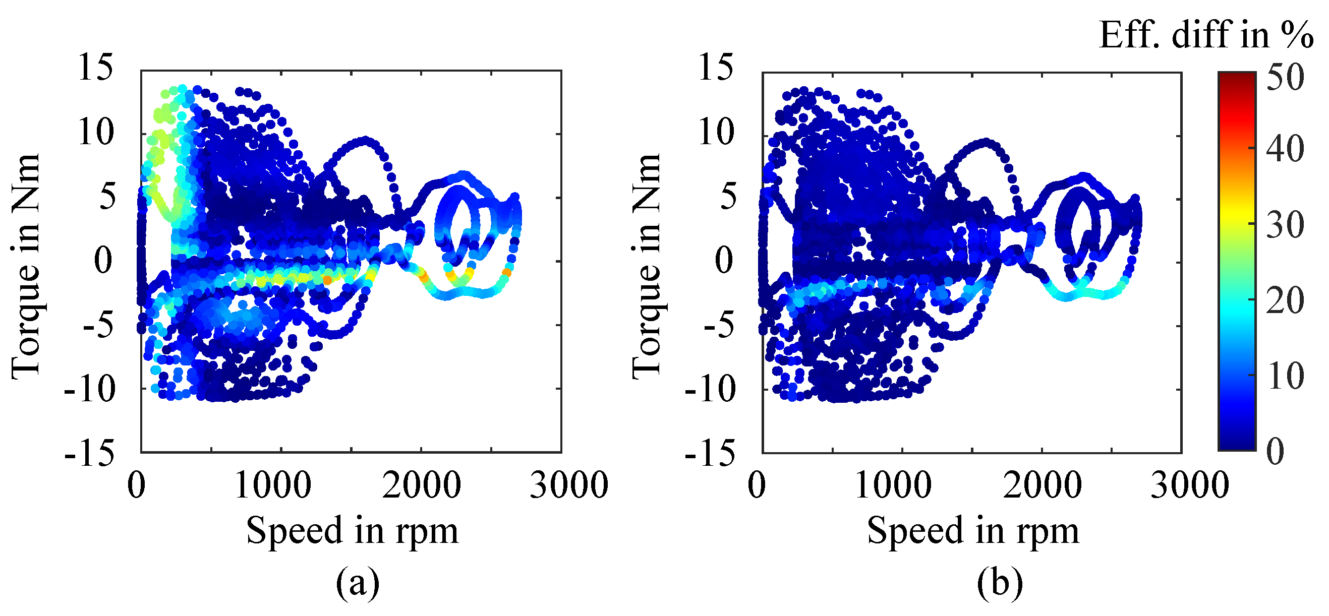
Figure 15.
Reference and measured torque-speed OPs for: (a) grid g4 (88×2), and (b) grid g5 (113×2).
Figure 15.
Reference and measured torque-speed OPs for: (a) grid g4 (88×2), and (b) grid g5 (113×2).
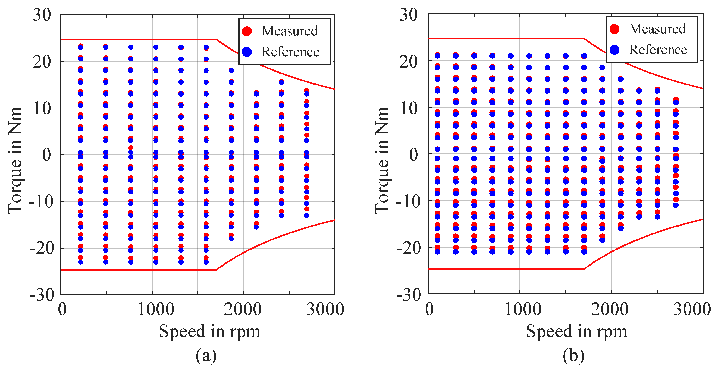
Figure 16.
Efficiency map differences obtained using grid g5, showing comparisons between: (a) measurement and analytic, (b) measurement and FEA, and (c) FEA and analytic.
Figure 16.
Efficiency map differences obtained using grid g5, showing comparisons between: (a) measurement and analytic, (b) measurement and FEA, and (c) FEA and analytic.
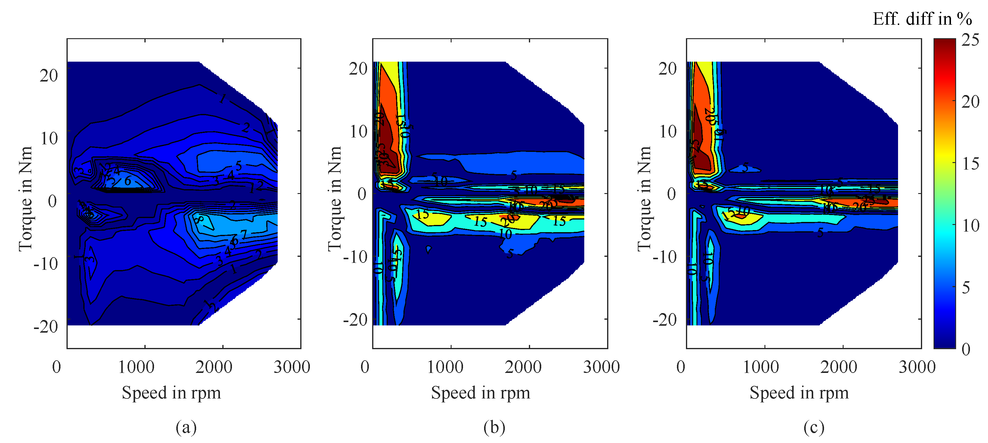
Figure 17.
Quantification of grid interpolation error for different torque-speed placements.
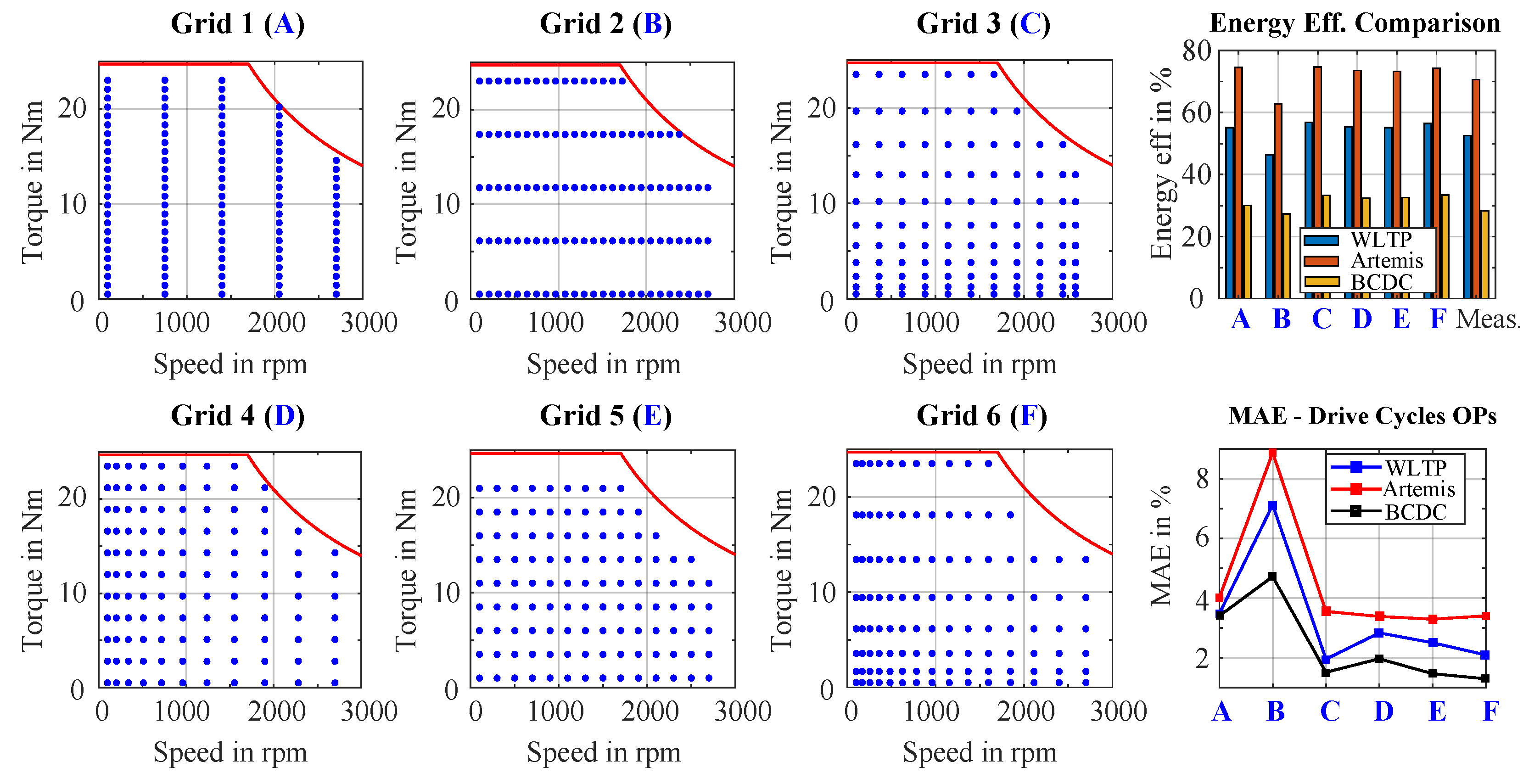
Figure 18.
Efficiency maps of the IM for (a) 20 °C and (b) 100 °C; obtained from the analytic model; from grid g5.
Figure 18.
Efficiency maps of the IM for (a) 20 °C and (b) 100 °C; obtained from the analytic model; from grid g5.
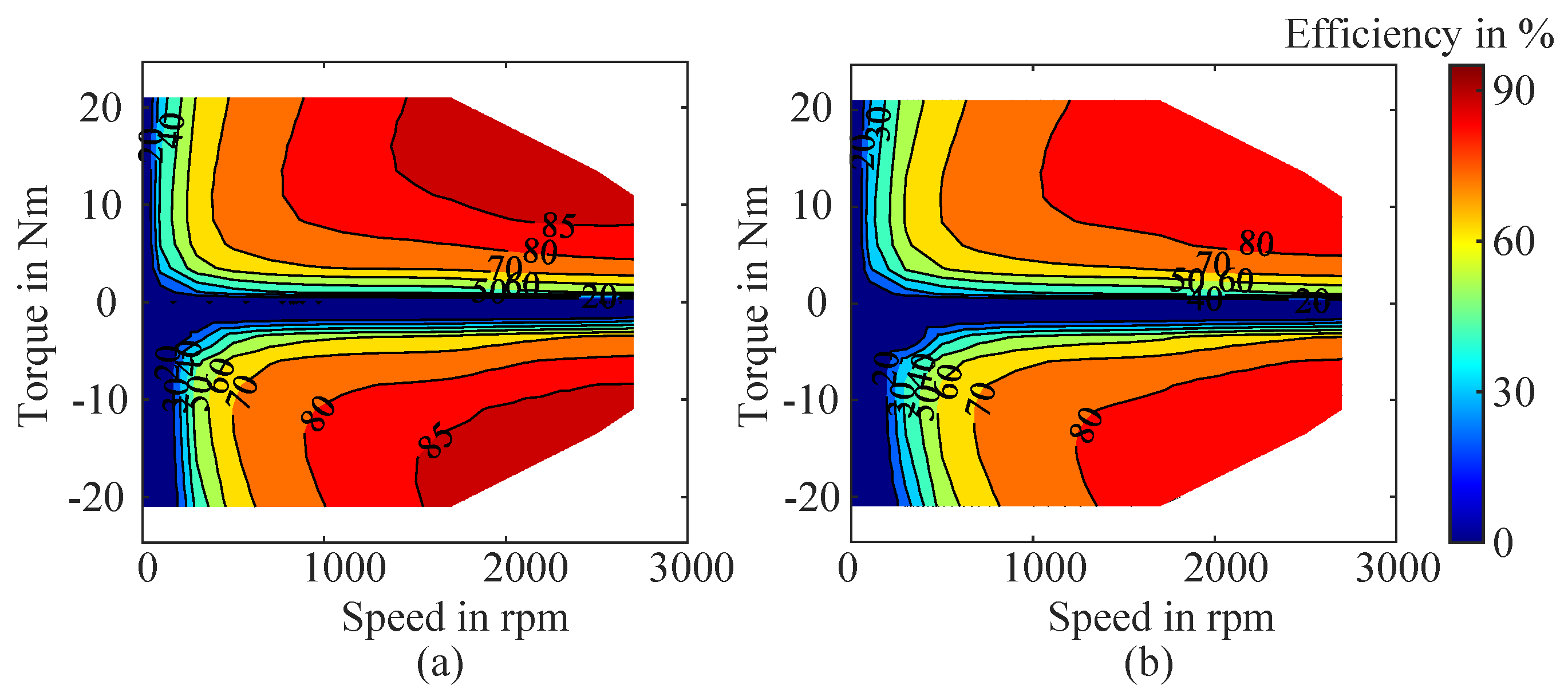
Figure 19.
Measured IM components temperatures during down-scaled WLTP drive cycle (based on the BMW i3).
Figure 19.
Measured IM components temperatures during down-scaled WLTP drive cycle (based on the BMW i3).
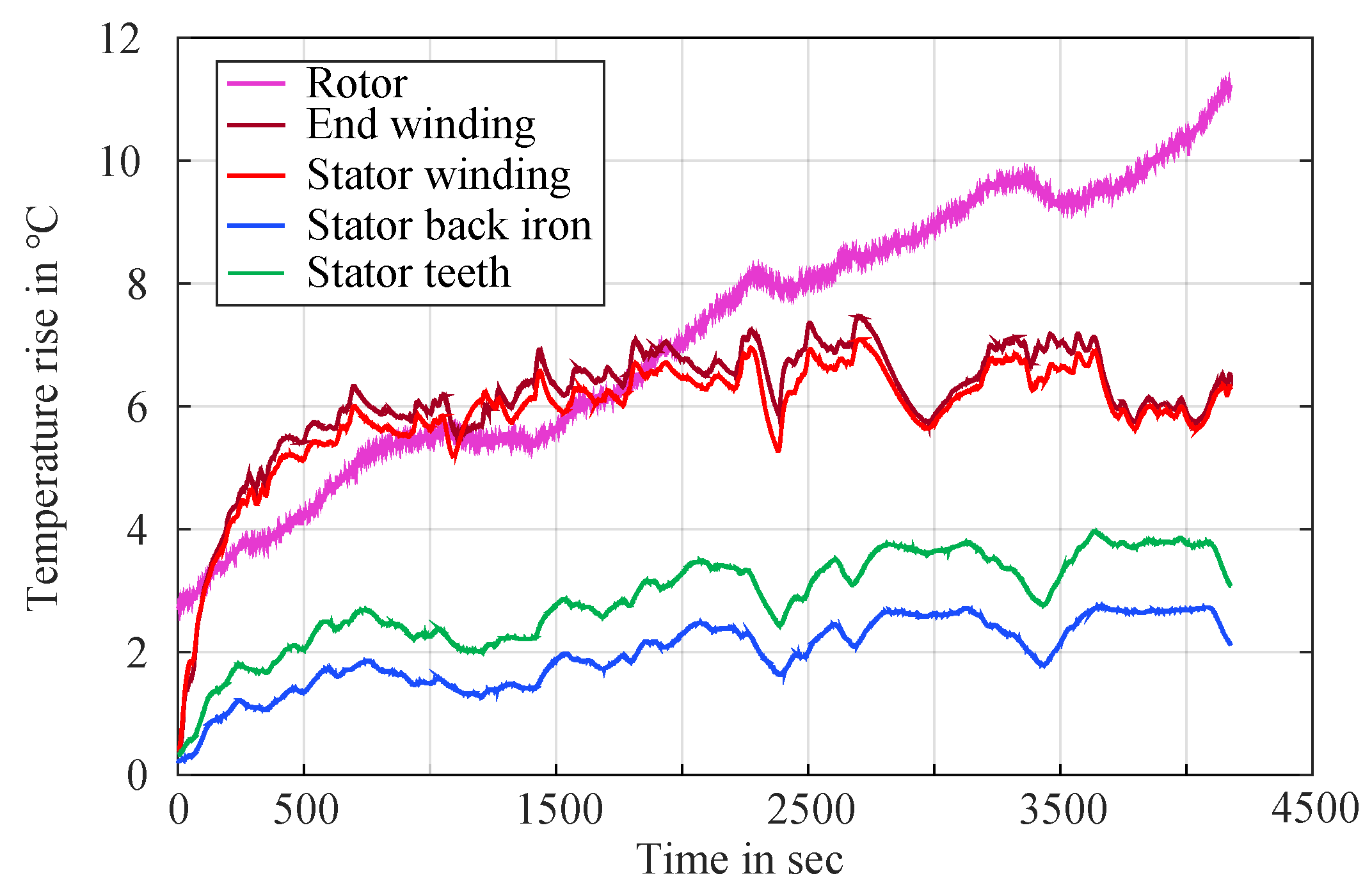
Figure 20.
Trade-off between grid size, simulation time, and MAE for down-scaled drive cycles (based on the BMW i3 ) using the FEA-based LUT method with five main grids (g1–g5).
Figure 20.
Trade-off between grid size, simulation time, and MAE for down-scaled drive cycles (based on the BMW i3 ) using the FEA-based LUT method with five main grids (g1–g5).

| Specifications of Vehicle Motors | ||
|---|---|---|
| Parameters | Vehicles | |
| BMW i3 | Smart EQ | |
| Max. Power | 125 | 60 |
| Max. Torque | 250 | 160 |
| Rated Speed | 4800 | 3600 |
| Maximum Speed | 11400 | 11475 |
| Laboratory Motor Specification | ||
| Parameters | Values | |
| Max. Power | 4.4 | |
| Max. Torque | 24.7 | |
| Rated Speed | 1430 | |
| Maximum Speed | 2850 | |
Table 2.
Summary of each down-scaled drive cycle’s input energy (), output energy (), and the corresponding efficiency ().
Table 2.
Summary of each down-scaled drive cycle’s input energy (), output energy (), and the corresponding efficiency ().
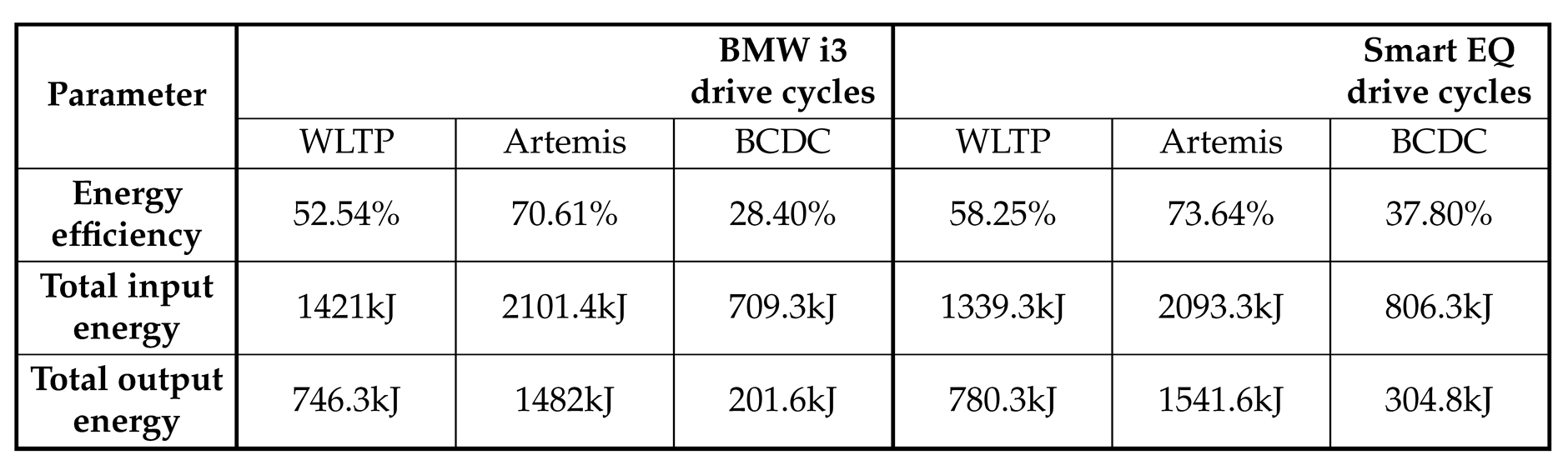 |
Table 3.
Drive cycle energy efficiency for each method and grid, based on mid- and small-range vehicle drive cycles.
Table 3.
Drive cycle energy efficiency for each method and grid, based on mid- and small-range vehicle drive cycles.
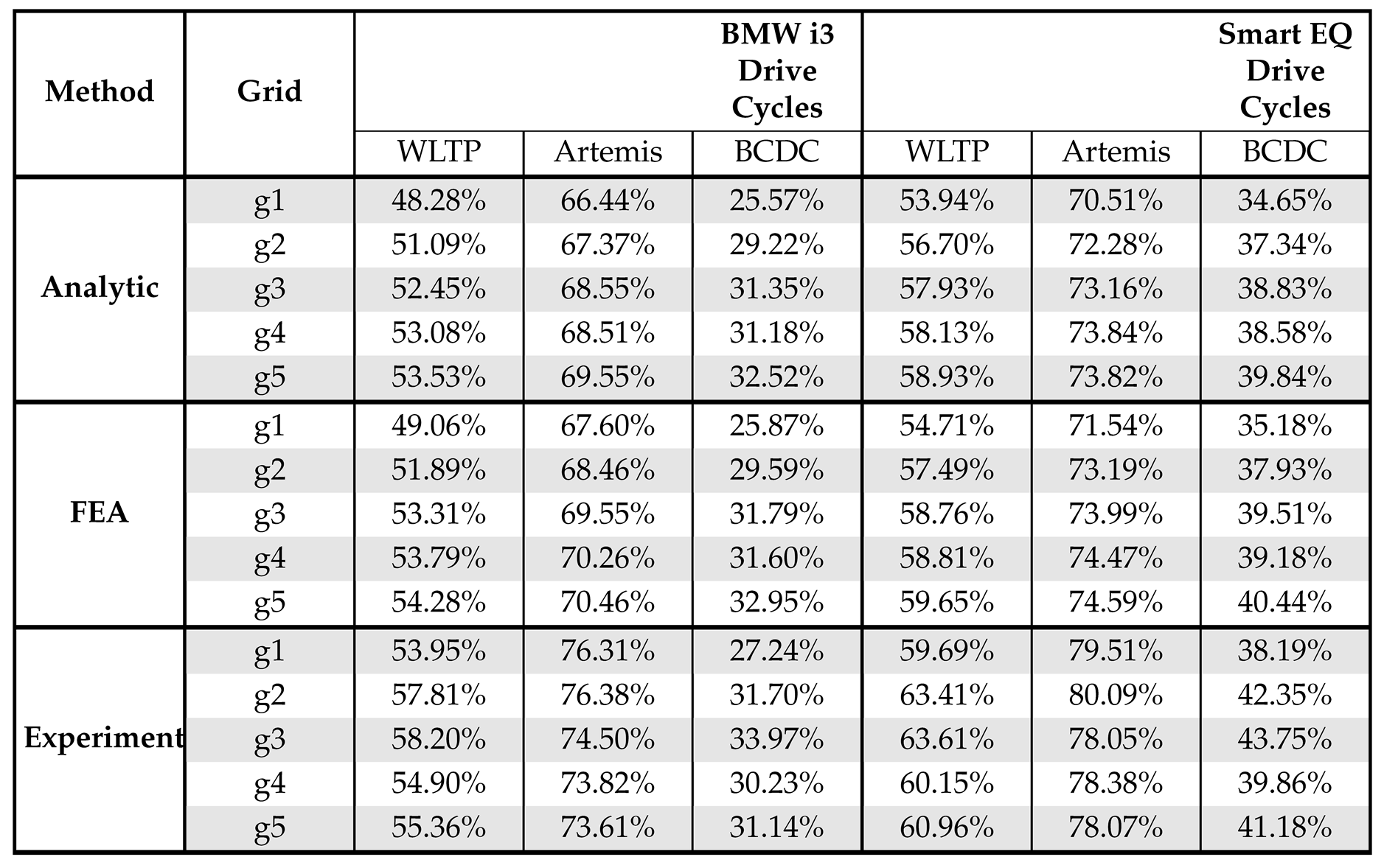 |
Table 4.
Results of the direct time-stepping analytic method, including drive cycle energy conversion efficiencies for the down-scaled drive cycles and the mean absolute efficiency error of the IM’s OPs compared to laboratory measurements.
Table 4.
Results of the direct time-stepping analytic method, including drive cycle energy conversion efficiencies for the down-scaled drive cycles and the mean absolute efficiency error of the IM’s OPs compared to laboratory measurements.
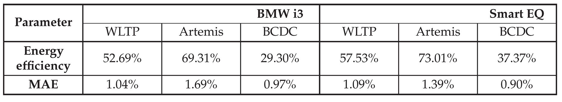 |
Table 5.
Mean absolute efficiency error of the IM’s OPs for each method and grid, across down-scaled drive cycles based on from mid- and small-range vehicles, compared to laboratory measurements.
Table 5.
Mean absolute efficiency error of the IM’s OPs for each method and grid, across down-scaled drive cycles based on from mid- and small-range vehicles, compared to laboratory measurements.
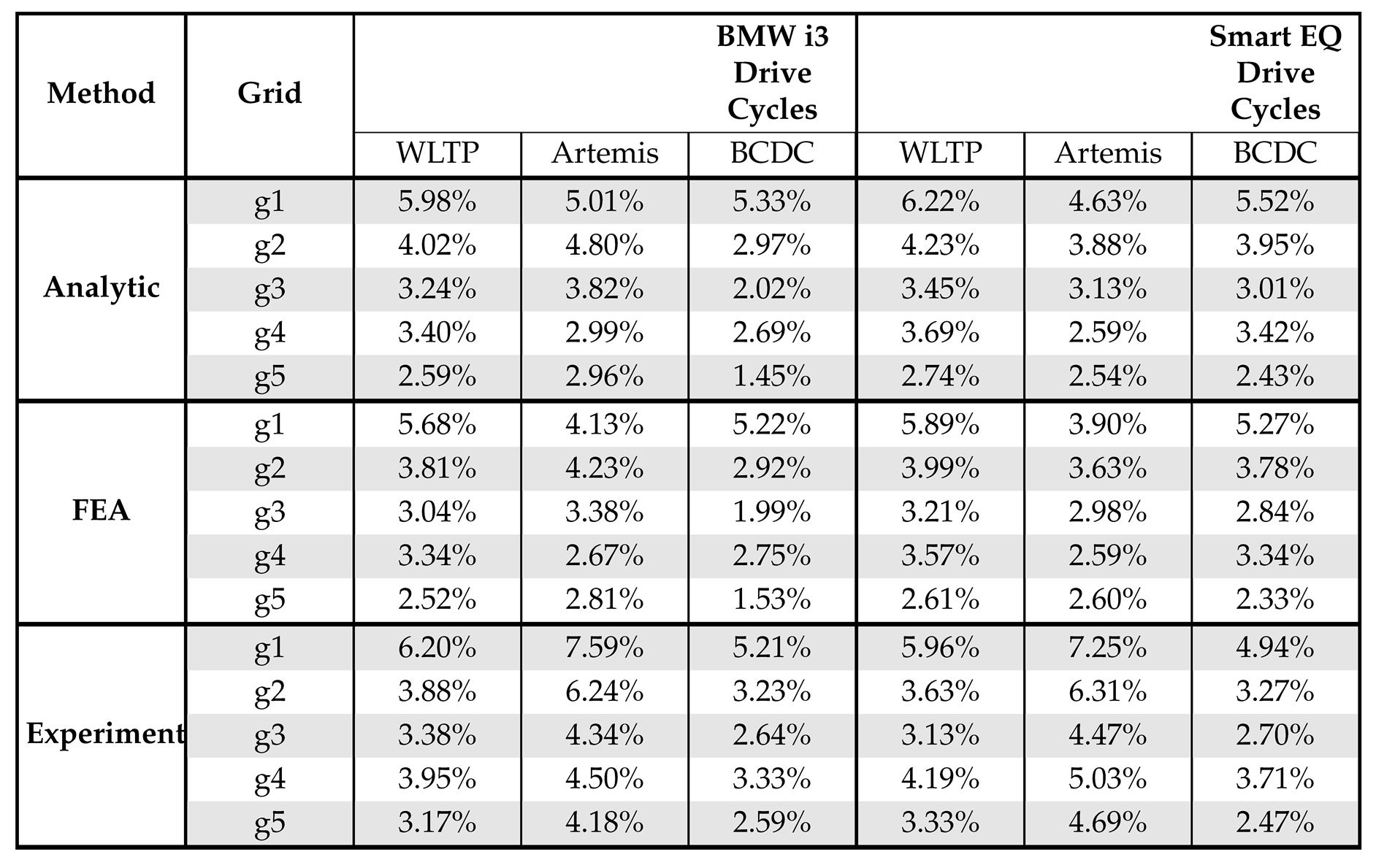 |
Table 6.
Impact comparison of factors affecting efficiency prediction accuracy in LUT-based and time-stepping methods for the IM.
Table 6.
Impact comparison of factors affecting efficiency prediction accuracy in LUT-based and time-stepping methods for the IM.
| Factors | LUT-based | Time-stepping |
|---|---|---|
| Interpolation errors | ⬤⬤⬤⬤⬤ | ◯◯◯◯◯ |
| Reference vs. measured OPs in experimental LUT method |
⬤⬤⬤◯◯ | ◯◯◯◯◯ |
| Friction and mechanical loss modeling |
⬤⬤⬤⬤◯ | ⬤⬤⬤◯◯ |
| Thermal effects and mismatch | ⬤◯◯◯◯ | ⬤◯◯◯◯ |
| Inaccurate iron loss modeling | ⬤⬤⬤◯◯ | ⬤⬤⬤◯◯ |
| Control strategy differences | ⬤◯◯◯◯ | ⬤◯◯◯◯ |
| Mesh quality in FEA | ⬤◯◯◯◯ | ◯◯◯◯◯ |
Table 7.
Comparison of Computational Times for Different Methods.
| Method | Grid | No. of Points | Simulation Time |
|---|---|---|---|
| Direct Analytic | – | 3600 (WLTP) | 8 min |
| – | 2136 (Artemis) | 4 min | |
| – | 3480 (BCDC) | 7 min | |
|
LUT-based Analytic |
g1 | 22×2 | 7s |
| g2 | 44×2 | 15 s | |
| g3 | 66×2 | 22 s | |
| g4 | 88×2 | 30 s | |
| g5 | 113×2 | 38 s | |
|
LUT-based FEA |
g1 | 22×2 | 21 min |
| g2 | 44×2 | 38 min | |
| g3 | 66×2 | 60 min | |
| g4 | 88×2 | 76 min | |
| g5 | 113×2 | 98 min | |
|
LUT-based Experiment |
g1 | 22×2 | 22.5 min |
| g2 | 44×2 | 44.5 min | |
| g3 | 66×2 | 66.5 min | |
| g4 | 88×2 | 88.5 min | |
| g5 | 113×2 | 113.5 min |
Disclaimer/Publisher’s Note: The statements, opinions and data contained in all publications are solely those of the individual author(s) and contributor(s) and not of MDPI and/or the editor(s). MDPI and/or the editor(s) disclaim responsibility for any injury to people or property resulting from any ideas, methods, instructions or products referred to in the content. |
© 2025 by the authors. Licensee MDPI, Basel, Switzerland. This article is an open access article distributed under the terms and conditions of the Creative Commons Attribution (CC BY) license (http://creativecommons.org/licenses/by/4.0/).
Copyright: This open access article is published under a Creative Commons CC BY 4.0 license, which permit the free download, distribution, and reuse, provided that the author and preprint are cited in any reuse.


