
Submitted:
12 December 2025
Posted:
17 December 2025
You are already at the latest version
Abstract
Self-organizing open systems, sustained by continuous fluxes between sources and sinks, convert stochastic motion into structured efficiency, yet a first-principles explanation of this transformation remains elusive. We derive the time-dependent Average Action Efficiency (AAE)—defined as events per total action—from a stochastic–dissipative least-action principle formulated within the Onsager–Machlup and Maximum Caliber path-ensemble frameworks. The resulting Lyapunov-type identity links the monotonic rise of AAE to the variance of action and to the rate of noise reduction, delineating growth, saturation, and decay regimes. Self-organization emerges from a reciprocal feedback between dynamics and structure: the stochastic dynamics concentrates trajectories around low-action paths, while the resulting structure, through the evolving feedback precision parameter β(t), modulates subsequent dynamics. This self-reinforcing coupling drives a monotonic increase of the dimensionless Average Action Efficiency αt =η/⟨ I⟩t , providing a quantitative measure of organizational growth. In the deterministic limit, the theory recovers Hamilton’s Principle. The increase of AAE corresponds to a decrease in path entropy, yielding an information-theoretic complement to the Maximum Entropy Production and Prigogine–Onsager variational formalisms. The framework applies to open, stochastic, feedback-driven systems that satisfy explicit regularity conditions. In Part II, agent-based ant-foraging simulations confirm sigmoidal AAE growth, plateau formation, and robustness under perturbations. Because empirical AAE requires only event counts and integrated action, it offers a lightweight metric and design rule for feedback-controlled self-organization across physical, chemical, biological, and active-matter systems.
Keywords:
self-organization
; stochastic thermodynamics
; least-action principle
; path integrals
; lyapunov functional
; nonequilibrium statistical physics
; dynamics
; structure
; open system
; path entropy
; maximum caliber principle
; maximum entropy production principle
; feedback-controlled systems
; active matter
1. Introduction.
Why do systems naturally increase their order? Spontaneous self-organization in complex systems—whether in convective flows, chemical oscillations, insect colonies, or neural networks—represents a remarkable convergence of physical laws and emergent dynamics. Understanding how structure emerges from the interplay between stochasticity, feedback, and dissipation is a foundational problem in nonequilibrium statistical physics. Conventional macroscopic metrics such as entropy production, mutual information, fitness functions, or order parameters are extremely useful, but often lack a universal, dimensionless form or a variational–dynamical foundation and can be non-monotone under feedback. We derive a dimensionless, action–based time-dependent efficiency metric whose monotonic rise quantifies path-space organization under the Maximum Caliber (MaxCal) principle. Under appropriate steady-state boundary or flux constraints, the formalism remains compatible with MEPP interpretations.
The stochastic–dissipative least–action framework applies to open systems sustained by continuous fluxes of energy or matter between a source and a sink. These fluxes define the boundary conditions of the variational problem and constitute the operational definition of openness in this formalism. In contrast, a closed system—with no maintained fluxes or distinct endpoints—reduces to the equilibrium limit, in which all microstates become equally probable and the formalism yields maximal internal (Boltzmann) entropy. The open boundaries define the domain of possible fluxes, while each event corresponds to one agent’s crossing of that flux channel; self-organization then manifests as the reduction of average action per crossing through feedback-driven concentration of trajectories.
We formalize self-organization within a canonical path ensemble, where each system trajectory carries an action and is weighted by a time-dependent precision factor that reflects feedback strength or inverse noise. The ensemble-averaged action defines a dimensionless efficiency , which rises monotonically as feedback concentrates trajectories around lower-action paths. This framework links stochastic thermodynamics, variational mechanics, and information theory within a single formalism.
Several routes have been explored previously: Stochastic thermodynamics links path probabilities to entropy production and fluctuation theorems [1]; The Maximum-Entropy-Production Principle (MEPP) has been invoked for steady states [2,3] and has been proposed as an inference from Jayne’s formalism [4]; Variational extensions of the least-action principle—Onsager–Machlup (OM), Graham, Freidlin–Wentzell—suggest that probable trajectories extremize generalized actions [5,6,7]. OM and Graham formulations sometimes include divergence or Jacobian corrections whose local sign is indefinite, but the quadratic large-deviation “cost” is nonnegative. Freidlin–Wentzell rate functionals are nonnegative by construction. Action minimization has been proposed to yield the MEPP under restricted NESS conditions [3]. Beyond classical OM/Graham/Freidlin–Wentzell, a modern variational formulation for open, dissipative systems shows that irreversible processes and boundary exchanges (mass/heat ports) can be derived directly from a constrained action principle [8]. The previous formalisms weight stochastic trajectories by an action functional. Building on the open–system structure [8] but within a stochastic path–ensemble framework, we extend the variational formalism to maintained flux networks: trajectories traverse explicitly defined source–sink boundaries, events are counted as individual crossings, and self-organization emerges as a reduction of average action per event under feedback.
While several Lyapunov functionals have been formulated for stochastic systems—typically in terms of state-space probability densities such as entropy or free energy—AAE is a dimensionless Lyapunov functional derived directly from a stochastic action integral and the corresponding path-ensemble measure, rather than from state-space probabilities. The Onsager–Machlup formalism [5] itself operates in path space: it assigns a probability density functional to entire stochastic trajectories rather than to instantaneous states. In the present framework, this stochastic–variational structure is extended to open systems with feedback and event-level normalization, yielding a path-ensemble measure analogous in form but distinct in physical scope. It extends it to open systems with source–sink boundaries and feedback-driven evolution and complements the Glansdorff–Prigogine formulation [9,10] by establishing explicit monotonicity of the ensemble-average action under feedback-driven precision increase. Unlike the classic Jarzynski [11] and Hatano–Sasa [12] functionals—whose uncorrected forms are not guaranteed to be monotone under feedback, since feedback requires information–theoretic corrections—the AAE remains monotone in the self–organization regime. It rises monotonically until saturation as feedback strengthens and the stated conditions hold.
This complements feedback fluctuation theorems [13,14] by providing a path-action–based Lyapunov functional tied directly to the canonical ensemble. This rise is governed by the variance of the action distribution and the time-dependent noise level in the system, thereby linking microscopic trajectories with macroscopic organization. AAE could solve the critical problem of quantifying self-organization in transient regimes, enabling variational design of feedback-controlled systems. We report experimental consistency in biological systems such as ATP synthase, with validation in agent-based simulations in Part II.
Empirically and theoretically, self-organized structures are often selected for their thermodynamic efficiency: they create channels that dissipate otherwise inaccessible free energy and are thus favored under the given drives and boundaries [15]. Conceptually, what counts as “self-organization”—routes, detection, complexity, and domain dependence—remains debated [16]. We adopt an open-system, boundary-aware view consistent with these discussions, focusing on feedback-driven concentration of trajectories and a dimensionless AAE.
Existing diagnostics for self-organization are primarily state–space based (e.g., KL- and entropy-production measures) and lack a unified, first-principles, path-action measure with a provable Lyapunov property under feedback. To our knowledge, no dimensionless, path–action–based metric has been formulated whose monotonic increase is derived directly from the canonical weighting and linked to feedback-driven precision () under explicit assumptions (C1)–(C7) (conditions). This absence limits principled, cross-system quantification of self-organization in open, stochastic, feedback-controlled regimes—where state-space measures such as Kullback–Leibler divergence or entropy production do not yield a guaranteed Lyapunov behavior.
Here we derive a path–integral observable—the Average Action Efficiency (AAE, denoted )—interpreted as the number of productive system events per total physical action, and prove that it acts as a Lyapunov functional in feedback–driven self–organization (1) under a well–defined set of conditions. The AAE serves as a model–agnostic, dimensionless, and variationally grounded metric for quantifying organization in systems that satisfy the canonical path–ensemble assumptions (C1)–(C7) (Section 4.1). Within its domain of validity, the Stochastic–Dissipative Average Action Principles yield an identity linking the rate of efficiency increase to the ensemble action variance and the rate of noise reduction, defining three dynamical regimes: growth, steady plateau, and decay. These regimes arise generically from the feedback-driven Lyapunov identity and do not depend on system-specific details, offering a common variational mechanism for the emergence of organization, stability, and decay across stochastic and dissipative domains. The narrowing of the path distribution under feedback corresponds to the system’s formation of structure, and in turn the structure influences the dynamics.
In the deterministic limit, the stochastic–dissipative framework naturally reduces to Hamilton’s principle. When noise and dissipation vanish (), the path ensemble collapses to the classical least-action trajectory with (Corollary 6). However, the theory is not intended for such deterministic cases, since the Lyapunov identity becomes trivial when the action variance vanishes.
From a MaxCal (maximum caliber) perspective, the canonical path weighting implies that the path entropy decreases whenever feedback increases effective precision, i.e., when [4,17,18]. Thus, the same mechanism that drives the Average Action Efficiency (AAE) to rise during self-organization corresponds to a monotonic drop in path entropy; at steady state both remain constant, and under disorganization the trends reverse. Interpreted purely inferentially, this MaxCal form expresses a statistical updating principle rather than a universal law [4,18,19]. However, when the feedback precision represents a real, measurable physical variable—such as signal-to-noise ratio, inverse temperature, or control gain—the same identity becomes a physically testable Lyapunov law governing self-organization dynamics. This theoretical result thus generalizes and justifies earlier empirical observations of increasing action efficiency across physical and biological systems [20,21,22].
Previous studies introduced empirical AAE through data and computational analyses, but lacked a path integral foundation [20,21,22,23,24,25,26]. The present study supplies its missing theoretical backbone. Earlier applications were limited to specific systems [20,21,22], while the current formulation expands the applicability across systems within the self-organization regime. These empirical and computational studies provided early evidence that systems under sustained feedback tend to increase their average action efficiency over time, hinting at an underlying variational mechanism now made explicit in the present formulation.
The present study establishes, within a unified stochastic–dissipative framework, the three canonical regimes of self–organization—monotonic rise, steady saturation, and decline—each corresponding to the sign of the feedback precision rate . Transient perturbations yield temporary deviations but preserve the Lyapunov property, leading to robust recovery once feedback resumes; persistent disturbances produce bounded fluctuations around a steady plateau determined by the balance of feedback and dissipation. Part I provides the theoretical derivation and analytical proofs of these regimes, while Part II will present simulation tests under both transient and continuous perturbations, confirming the predicted decline–and–recovery dynamics and quantifying system robustness. At this stage and within this framework, the Average Action Efficiency (AAE) serves as a complementary, dimensionless diagnostic—not a replacement—for traditional entropy- and information-based measures such as entropy production or free-energy dissipation.
Future work will extend the present framework beyond its current limitations, toward broader applicability and potential unification with established thermodynamic measures. Related manuscripts develop the –based formalism [27,28]. By explicitly linking the stochastic action to measurable energy or information fluxes, the Average Action Efficiency (AAE) could serve not only as a complementary diagnostic but, in certain regimes, as an alternative to conventional entropy- and free-energy–based metrics. Such extensions would establish AAE as a variationally grounded descriptor capable of bridging energetic, informational, and dynamical perspectives on self-organization, and of guiding future empirical tests across biological and engineered systems. Ultimately, this framework suggests that self-organization can be understood as the progressive concentration of stochastic dynamics toward paths of increasing average action efficiency—a process that links microscopic fluctuations to macroscopic order through a single variational mechanism. The following section develops the mathematical foundation of this framework by formulating the stochastic–dissipative action, its canonical path weighting, and the feedback-dependent ensemble dynamics from which the Lyapunov property of AAE arises.
These considerations suggest that self–organization cannot be understood solely as a consequence of external constraints or thermodynamic gradients, but must also involve an internal feedback between a system’s dynamics and its evolving structure. A defining feature of self–organizing systems is the reciprocal coupling—and consequent coevolution—of dynamics and structure. This coevolution follows from a stochastic–dissipative least–action principle that provides a variational mechanism for the emergence of order under nonequilibrium conditions. The stochastic dynamics of the system generates organized patterns by progressively concentrating trajectories around low–action paths, while the resulting structure, through the feedback parameter , modulates and constrains subsequent dynamics. This mutual dependence closes a causal loop in which dynamical laws give rise to organization, and the emerging organization feeds back to guide the motion of its constituents. Within the stochastic–dissipative formalism, this loop is expressed quantitatively through the evolution of the precision parameter , whose increase both suppresses fluctuations and drives the monotonic rise of the Average Action Efficiency. Thus, structure and dynamics co-determine each other: the dynamics “tells’’ the system how to organize, and the structure “tells’’ its constituents how to move.
2. Stochastic–Dissipative Action Framework
The classical least–action principle (LAP) applies to conservative, deterministic systems whose trajectories extremize an action functional under fixed boundary conditions [29,30], and emerges as a limiting case of this framework (Corollary 6). Self-organizing systems, by contrast, are open, stochastic, and dissipative: they exchange energy and matter with their surroundings and exhibit intrinsic fluctuations and structure formation. For such systems, the LAP must be extended to a probabilistic, ensemble-based framework in which trajectory weights reflect noise and dissipation. In this framework, all trajectories are in principle permitted, but those with larger stochastic action are exponentially suppressed, so the ensemble is overwhelmingly dominated by the minimum–action (most action efficient) paths. This generalization appears first in Onsager’s variational framework for near-equilibrium processes and in the Onsager–Machlup (OM) path weight for stochastic dynamics [5,31,32], and more broadly in large-deviation and stochastic-thermodynamic formulations [1,7,33].
In this ensemble view, each trajectory is assigned a stochastic–dissipative action functional , representing the physical action along the path—comparable to the dissipated energy–time product. For physical systems, typically scales with the total energy dissipated multiplied by the characteristic duration of a process, making it a direct measure of the physical “cost” of a trajectory. In special limits, reduces to the Onsager–Machlup stochastic action which measures the dynamical cost of a trajectory relative to its deterministic drift. It describes small deviations from equilibrium or, more generally, a stochastic variable following a Langevin equation:
where
- is the system’s state (e.g., concentration, velocity, position, order parameter, or generalized coordinate),
- is the deterministic drift or relaxation term (the “thermodynamic force”),
- D is the diffusion coefficient (noise strength), and
- is Gaussian Dimensionless, unit-variance white noise with correlation . Physical prefactors are absorbed into the definition of .
The Onsager–Machlup stochastic action functional measures how “costly” a particular trajectory is relative to the deterministic drift :
whose exponential weighting determines trajectory likelihoods [1,5]. The term penalizes deviations from deterministic motion. The prefactor sets how strongly the noise suppresses improbable paths. The Onsager–Machlup action functional is dimensionless: the prefactor removes all physical units, since D carries dimensions of . The integrand thus has dimension , and the time integral yields a dimensionless cost functional [1]. The path integral exponent must always be dimensionless, either by construction or by dividing by the Planck’s constant, as in Quantum Mechanics. This is because probabilities (and their amplitudes/weights) are inherently dimensionless. Smaller means a more probable trajectory. Paths with larger are exponentially suppressed as . In the small–noise limit, acts as a positive–definite “dynamical potential” whose minimum corresponds to the most probable trajectory.
More general nonlinear forms, including those developed by Graham and co-workers, extend the action to systems far from equilibrium [6]. This formulation replaces deterministic trajectories with probability-weighted histories, allowing the least-action concept to survive in stochastic, dissipative contexts. It reframes organization as the statistical dominance of low-action trajectories rather than as a purely mechanical extremum.
The increase of probability for lower-action trajectories under stochastic and dissipative dynamics defines a Stochastic–Dissipative Least Action Principle (SDLAP) - the paths with least action are the most probable. In the present formulation, this stochastic action is further extended to incorporate explicit feedback control and ensemble averaging, forming the basis of the Stochastic–Dissipative Least Average Action Principle (SD–-LAAP). This establishes a conceptual lineage:
This hierarchy of principles illustrates a continuous generalization of classical mechanics: from deterministic extremal paths to stochastic ensembles whose organization is governed by feedback and dissipation. Each successive formulation introduces one new degree of realism: the Onsager–Machlup action incorporates stochasticity and dissipation (SDLAP), while the present Stochastic–Dissipative Least Average Action Principle (SD–LAAP) adds feedback and ensemble adaptation through the time–dependent precision parameter .
In the stationary case, the path probability distribution is given by
where quantifies system noise and denotes the path integral measure over all trajectories [7]. The normalization condition ensures that probabilities sum to one and defines the partition functional:
The scale parameter carries the same physical units as the action and may depend on the system or state; for instance, in thermal systems or in diffusive dynamics. The exponential argument is therefore dimensionless, and the form remains valid for any consistent choice of and . More generally, it reflects an effective fluctuation scale or cost parameter. The ensemble average action
serves as a reference for disordered states and converges to the OM thermodynamic action in the linear-response regime, where it reflects the dominant contribution to entropy production and path likelihoods [1,34]. inherits the same dimensions as .
We introduce the time-dependent precision parameter , so that small noise levels correspond to large precision and hence stronger exponential concentration around low-action trajectories. quantifies feedback strength and, in the small–noise limit, plays the role of an inverse noise scale [5,7,33,35]. In stochastic thermodynamics, this is the standard path–weighting underlying large deviations and Fokker–Planck dynamics. For the Onsager–Machlup form in Eq. (2), , hence . This mapping connects the stationary ensemble of Eq. (3) with the time–dependent path measure in Eq. (6).
While Eq. (3) describes stationary ensembles under fixed noise levels (), real self-organizing systems operate under time-dependent drives and feedback, for which the effective precision evolves dynamically, coupling microscopic fluctuations to macroscopic organization. This ensemble construction provides the foundation for describing how feedback modifies the statistical weighting of trajectories and, consequently, how organization emerges from stochastic dynamics. It establishes the mathematical bridge between traditional least-action principles and the time-dependent feedback formalism developed in the next section.
3. Time-Dependent Dynamics
In open, driven systems with weak noise, the time-dependent path ensemble evolves from an initially broad distribution toward exponential concentration around least-action trajectories, as described by large-deviation theory [7,33]. The corresponding steady-state path measures and endpoint probabilities are determined by boundary conditions (sources and sinks) and by the non-equilibrium steady currents that they sustain, as formulated in Fokker–Planck dynamics [35,36]. When feedback control is present, the weighting of trajectories is further reshaped in accordance with information–thermodynamic constraints and generalized nonequilibrium equalities that incorporate measurement and feedback [1,13,37,38].
The stochastic action quantifies the total cost of a trajectory—integrating energy expenditure and duration. For biological or agent-based systems, I may represent kinetic-energy dissipation or metabolic work per productive event. Let be a fixed (time-independent) action functional defined over trajectories , and let the instantaneous path distribution be
with normalization
In this formulation, quantifies how feedback reshapes the probability landscape of possible trajectories, while measures the ensemble’s overall diversity. A decrease in under growing corresponds to the ensemble’s contraction around low-action trajectories, providing a natural measure of increasing organization in path space. This is analogous to a partition function in statistical mechanics [1,5,7,33,39]. The larger , the less organized the ensemble [40,41]. The formalism parallels equilibrium statistical mechanics, but with the “energy” of a state replaced by the action , and a time-dependent precision parameter that evolves under feedback. Hence, the partition function of a self-organizing system describes not static configurations but the ensemble of possible histories under fixed control parameters , averaging protocol , and event definition , defined below.
Throughout this work, three sets of specifications define the context of the path ensemble— fixes what the system is, defines how we observe it, and defines what it does—that jointly determine its scope:
- — the control and boundary parameters of the system, such as geometry, nodes, external driving, material constants, and, in open systems, the specification of the source and sink manifolds and that maintain flux and define the boundary conditions for admissible trajectories. Examples include in Rayleigh–Bénard convection or in the two-path foraging model.
- — the averaging protocol, describing how ensemble quantities are evaluated. It specifies the time window , ensemble type (temporal, spatial, or agent-based), and coarse-graining rule used to compute or . In theoretical formulations, serves only as a formal prescription for ensemble averaging, while in empirical or computational implementations it specifies the actual measurement or sampling procedure.
- — the definition of a productive event, identifying what counts as one completed functional cycle in the system. In this framework, one event corresponds to one abstract crossing between a source and a sink by a single agent of the system, for example one foraging trip between food and nest, one circulation of a convection roll transporting heat from the hot to the cold plate, or one ATP molecule synthesized per completed proton-driven catalytic cycle.
One considers the state space specification: system variables, resolution level, observable definitions, and coarse-graining and also the feedback specification: feedback mechanism, delay times, nonlinearities, and information processing rules. Each trajectory is a continuous path in the system’s state space (e.g., positions, velocities, or concentrations), with observables defined as functionals of under a fixed coarse-graining resolution consistent with . The stochastic dynamics underlying are assumed to be driven by Gaussian white noise, corresponding to Markovian diffusions with a well-defined variance parameter (or diffusion coefficient D). This assumption underlies the Onsager–Machlup construction; extensions to colored or multiplicative noise require modified path measures beyond the present scope.
Details such as finite response delay, nonlinear saturation, or information-processing mechanisms are system-specific and excluded under the present smooth-feedback assumption (C1). The averaging protocol includes specification of the initial ensemble , which sets the reference state from which self-organization proceeds. Unless stated otherwise, we assume finite normalization and that transient equilibration before establishes a reproducible initial distribution.
Together with the specified form of the stochastic action , fully determine the ensemble context [1,5]. Once is chosen and are fixed, the path probability and all derived quantities are uniquely defined. Finer specifications (state space resolution, noise characteristics, feedback implementation details) are held fixed within this macroscopic framework. Just as temperature, volume, and particle number specify the statistical ensemble in equilibrium thermodynamics, these quantities determine the macroscopic boundary within which trajectories evolve and feedback operates. Altering any of them changes the admissible set of trajectories and, consequently, the interpretation of the ensemble averages and . In particular, variations in correspond to external driving or boundary control, whereas changes in or correspond to different observational resolutions or definitions of functional events. Maintaining these specifications fixed during analysis ensures that the observed monotonicity in arises from intrinsic feedback dynamics rather than from redefinition of the ensemble itself.
has a concrete physical interpretation: it quantifies how feedback modulates the system’s effective noise level. When increases, stochastic fluctuations are progressively suppressed, and the ensemble becomes increasingly concentrated around energetically or dynamically efficient paths. Conversely, when decreases, fluctuations dominate and organization erodes. Thus, serves as the control parameter governing transitions between disorder, self–organization, and disorganization.
Positive feedback can effectively raise by reducing fluctuations: in ant foraging, pheromone reinforcement biases headings and amplifies low–action routes [42,43,44]; in molecular machines, regulation under load suppresses slippage and narrows trajectory ensembles [1,45]. With explicit feedback control, trajectory reweighting is constrained by information–thermodynamic relations and feedback fluctuation equalities [13,14].
Therefore, throughout, we treat as time–independent under fixed coefficients and boundary conditions, so that changes in arise via the feedback–driven [7,33]. In this formulation, encodes the microscopic dissipative dynamics—the friction, diffusion, or energetic cost defining the local stochastic process—whereas represents a macroscopic, feedback-controlled precision scale[1,5] that governs how sharply the ensemble discriminates among trajectories [13,14]. Thus, dissipation enters the theory only once—through —while modulates the degree to which feedback suppresses stochasticity at the ensemble level.
4. Self-Organization
Having established the stochastic–dissipative action framework, we now formulate the conditions and dynamical laws that govern self-organization. In this section, the probabilistic least–action formalism is specialized to feedback–driven open systems, where the ensemble evolves under time–dependent precision . The goal is to identify the precise mathematical assumptions under which the system’s average action decreases and its average action efficiency increases—thereby defining self-organization in operational and variational terms. These foundational conditions provide the starting point for the Lyapunov derivation that follows.
4.1. Foundational Conditions for Self-Organization Valid for all
Before deriving the dynamical results, it is necessary to specify the foundational conditions under which the stochastic–dissipative formulation is mathematically and physically well posed. These conditions play a role analogous to the smoothness, boundedness, and normalizability assumptions that accompany the derivation of the Fokker–Planck equation or large–deviation principles. They ensure that path integrals converge, that derivatives with respect to time are well defined, and that the feedback parameter produces a stable evolution of the ensemble. Each assumption has a clear physical meaning—bounded noise, finite dissipation, and differentiable feedback—and violations of them correspond to singular or noncanonical regimes such as discontinuous control, diverging fluctuations, or unbounded domains. The conditions are valid for the following cases.
4.1.1. Open Systems = Specified Source–Sink Boundary Conditions
In the stochastic–dissipative least–action framework, the endpoints of trajectories are defined by the open nature of the system. An open system is one in which there exists a source (where energy or matter enters the system) and a sink (where dissipation or output occurs). Every trajectory is therefore a channel connecting those two boundary manifolds,
In this sense, self–organization is a form of flux organization: the system develops structures that minimize the average action given those boundary fluxes. The boundaries are not passive; they maintain the system far from equilibrium and thereby define the context for minimization. The system is open and maintains continuous fluxes between a source and a sink , which define the boundary conditions for all admissible trajectories . These boundaries maintain the system far from equilibrium and give directionality to the least–action minimization. In the absence of such fluxes (closed system), all endpoints become statistically equivalent, approaches a uniform distribution over accessible microstates, and the variational structure reduces to the equilibrium limit of maximal Boltzmann entropy.
Here denote an individual trajectory in the ensemble, with and specifying its open boundary conditions. The ensemble measure in subsequent equations integrates over all such admissible trajectories. The sets and denote the source and sink manifolds in the system’s configuration space. They specify the open boundary conditions that define the admissible domain of trajectories in the ensemble. Each trajectory begins at some point , where energy or matter enters the system, and terminates at , where dissipation or output occurs. These boundary manifolds can be discrete (e.g., two spatial points, as in the case of an ant moving between a food source and a nest) or continuous hypersurfaces (e.g., isothermal or isopotential boundaries in a thermal or electrochemical system). These may represent, for example, a hot reservoir and a cold reservoir, a nutrient supply and a waste removal region in an ecological setting. In general, they represent the regions of state space through which external fluxes maintain the system far from equilibrium.
In physical terms, corresponds to the locus of all possible input states, where the system receives external driving or free energy, while represents the locus of output or dissipative states, where the system exports entropy or releases energy to the environment. The continuous supply of flux between these two boundaries sustains the system in a nonequilibrium steady regime and defines the directionality of all admissible paths. In this sense, the openness of the system is expressed not merely by boundary terms in the energy balance, but by the geometric constraint that all trajectories connect to . This geometric formulation directly parallels the flux boundary conditions in nonequilibrium thermodynamics, where gradients of temperature, chemical potential, or population density drive steady transport. In the present variational formalism, it ensures that action minimization and feedback evolution occur within an open domain in which sources and sinks continuously define the beginning and end of each event.
4.1.2. Variational Structure with Fixed Boundaries
This corresponds exactly to the classical least–action setup,
Even in the stochastic–dissipative generalization,
the normalization constant Z and all averages are conditional on those endpoints. They are constraints that make the path measure non–uniform and give meaning to “low action.” When the boundaries are fixed, the canonical weighting drives probability concentration toward efficient flux paths — that is the statistical manifestation of self–organization.
4.1.3. Event Definition
A single event corresponds to one completed crossing between the source and sink by a single agent of the system. Within the stochastic–dissipative path ensemble, we can introduce an event indicator functional:
Each trajectory segment completing such a crossing contributes one unit to the event ensemble E, whose indicator functional equals unity for a completed crossing and zero otherwise. The ensemble–averaged number of events is then . This definition ensures that the Average Action Efficiency is normalized per productive flux–carrying transition.
The path integral is then understood as restricted to paths satisfying:
The crucial point is that the source–sink structure provides a directional bias in path space: trajectories must carry flux from to (or around a specified cycle), which breaks the symmetry among all possible endpoints.
4.1.4. Closed or Unbounded System → no Privileged Endpoints → Maximum Entropy
If the source and sink are removed, the boundary constraints disappear, and all endpoints (or equivalently, all regions in configuration space) become statistically equivalent. The only remaining constraint is normalization. In this limit, the same variational principle reduces to
because the uniform distribution over accessible microstates becomes the stationary measure. The least–action principle remains formally valid but becomes degenerate: all trajectories are equally probable, and no path structure is selected. The only surviving extremum condition is entropy maximization under the conservation laws. Thus, in the absence of flux boundaries, the least–action ensemble collapses into the equilibrium limit of maximum Boltzmann entropy. The system can no longer reduce its average action, because every microstate is equally likely to be visited.
4.1.5. Examples
We now illustrate the role of source–sink boundary conditions in several canonical self–organizing systems.
-
Ant foraging (nest–food system). Let denote the nest region and denote the food source. Each ant trajectory is a path that carries material flux (food) from back to via a round tripAt early times, when the pheromone field is uniform, many tortuous paths between nest and food have comparable probabilities, and the distribution of actions is broad. As ants deposit pheromone along successful, shorter paths, a positive feedback increases the effective : long, high–action trajectories are penalized, while short, low–action trajectories are reinforced. The boundary conditions (nest and food) remain fixed, but the ensemble collapses onto an efficient path network connecting them, reducing and increasing .If the nest and food were removed, so that there were no distinguished source–sink pair, the same random walkers would simply diffuse and asymptotically explore the accessible region of space; the action distribution would no longer be driven toward lower values by any flux constraint, and the system would approach a maximal–entropy spatial distribution rather than a self–organized trail.
-
Rayleigh–Bénard convection. In Rayleigh–Bénard convection, the lower plate at temperature acts as a thermal source, while the upper plate at acts as a sink. Fluid trajectories carry heat from the hot plate to the cold plate, subject to no–slip and temperature boundary conditions at the walls. When the Rayleigh number exceeds a critical value, the system self–organizes into convection rolls: coherent flow patterns that transport heat more efficiently than pure conduction. In terms of the present formalism, the plates define and , and the convective patterns correspond to a reweighting of path space toward low–action trajectories that accomplish the required heat flux with reduced dissipative cost.If the temperature difference were removed (), the system would lose its source–sink structure, no net heat flux would be required, and the fluid would relax to an equilibrium state with maximal entropy and no convective organization.
-
Biochemical cycles (e.g. ATP synthase). In biochemical machines such as ATP synthase, the proton–motive force (difference in electrochemical potential across a membrane) acts as a source of free energy, while the synthesis of ATP and its eventual hydrolysis in the cytosol represent sinks. Each catalytic cycle of ATP synthase is a trajectory in a high–dimensional conformational and chemical space that connects a source manifold (high proton free energy, ADP + ) to a sink manifold (lower proton free energy, ATP produced and exported). Over evolutionary and regulatory timescales, feedback tightens the coupling between proton flux and ATP production, increasing the effective precision and concentrating probability on low–action, tightly coupled pathways. This leads to high Average Action Efficiency at the level of catalytic events.If all chemical potentials were equalized and no free–energy gradient were maintained, the system would become effectively closed: no net proton flux, no net ATP production, and no directional bias in the space of chemical trajectories. The ensemble of molecular states would then relax toward a maximum–entropy distribution, and no sustained self–organization at the cycle level would be observed.
Conditions
Under these physical prerequisites, the following mathematical conditions ensure that the stochastic–dissipative formulation remains well posed for all :
- (C1)
- Regular feedback:. Ensures differentiability of and .
- (C2)
- Positive inverse noise:. Prevents divergence and ensures a well-defined path measure.
- (C3)
- Local normalizability: The normalization constant is finite for all t, and remains uniformly bounded in a neighborhood of each time point: Within any local time window, therefore never diverges—it stays bounded by some finite value.
- (C4)
- Strictly positive action:, , with no explicit time dependence. Ensures (in Alphat ) is finite and meaningful.
- (C5)
- Integrability: is finite because . Needed for defining (in Alphat ) and for well-posed ensemble averages.
- (C6)
- Strictly positive residual variance: and finite, due to unavoidable fluctuations (thermal, behavioral, or quantum).
- (C7)
- Fixed ensemble specifications during differentiation: held fixed on any time interval where derivatives and are taken.
The present formulation is valid only within these assumptions; systems that violate them lie outside the current theoretical scope. These conditions are standard in statistical mechanics and stochastic thermodynamics and guarantee mathematical regularity of the ensemble—finite normalization, differentiability, and integrability—which are necessary for the Lyapunov derivation [1,35,36]. They can later be relaxed systematically to treat evolving environments, adaptive feedback, nonstationary noise, and noncanonical path measures. Such extensions will require generalized formulations of the path weight, normalization, or differentiability conditions but do not alter the core structure established here.
Having established the regularity and boundedness conditions required for a well–defined ensemble, we now examine how the average stochastic action evolves in time under feedback. The quantity serves as the ensemble–level observable that captures how feedback progressively concentrates trajectories around lower–action paths. Its dynamics encode the balance between dissipation and precision, linking microscopic stochastic fluctuations to macroscopic organization. The resulting time derivative of provides the foundation for identifying Lyapunov behavior and quantifying self-organization.
4.2. Time-Dependent Average Action
The ensemble average action at time t is given by
and serves as a quantitative signature (observable) of organizational progress. We refer to it as a Stochastic-Dissipative Average Action Principle (SD–AAP). Since retains its physical dimensions under feedback, shares the same units and evolves continuously with . When sources and sinks are defined as endpoints, as the system self-organizes, becomes increasingly peaked around low-action trajectories, and decreases correspondingly [1,40,46]. At , the distribution is broad, approximating a uniform distribution over paths. Over time, positive feedback sharpens the distribution, reducing as the system transitions from disordered to organized states. This reduction in average action reflects the system’s increasing alignment with low-action trajectories.
To make this relation explicit, we now derive how feedback modifies the ensemble distribution and, consequently, the average action . Starting from the canonical path weighting and normalization, we obtain an exact identity linking changes in the partition functional to changes in . This derivation establishes the fundamental bridge between feedback precision , stochastic fluctuations, and the rate of self-organization. It culminates in a Lyapunov-type identity showing that increasing feedback precision monotonically decreases the ensemble-average action.
4.3. Dynamical Action Principle in Stochastic Dissipative Self-Organization
Lemma 1 (Path-weight identity).
Under (C1)–(C7), starting from the canonical normalization factor partition the only explicit time dependence is through , since is time–independent under assumption (C7). Differentiating with respect to t gives
Dividing both sides by yields
Recognizing the normalized path measure PathProbability, the ensemble average of the action is
Substituting eq:Imean into eq:dlnZintermediate gives the desired identity:
This expression shows that increasing (i.e., increasing precision or reducing noise) reduces the partition functional , reflecting the progressive concentration of the path ensemble around lower–action trajectories.
Thus with PathProbability and partition we have
Hence the path–weight identity is
Differentiating the ensemble average of the action as defined in EnsembleAv with respect to time gives
Using the previously derived path–weight identity, eq:path-weight-identity we substitute this into eq:dIavgstart:
Expanding the integrand gives
Recognizing the definitions
we simplify:
Finally, by definition of the ensemble variance,
we obtain the compact form:
which shows that whenever feedback increases (), the average action decreases—so the system self-organizes. represents a system learning or reinforcing efficient paths. decreases because feedback selectively suppresses high-action trajectories.
Reciprocal Coupling of Dynamics and Structure
Within the stochastic–dissipative least–action framework, the feedback precision mediates the reciprocal coupling between dynamics and structure. The system’s dynamics generates organization by concentrating its trajectories around regions of lower action, while the resulting structure, through changes in , modulates the effective noise level and thereby constrains subsequent dynamics. As increases, fluctuations are progressively suppressed and the ensemble of paths becomes more coherent; as decreases, fluctuations broaden the distribution and structure decays. This two–way dependence closes a causal loop in which dynamical evolution gives rise to structure, and the emerging structure feeds back through to regulate motion. In this formulation, functions as a macroscopic measure of feedback precision linking microscopic fluctuations to macroscopic organization.
Feedback Formalism and Monotonic Trends
The time dependence of determines the direction of organizational change. When the feedback strengthens (), the average action decreases over time, driving an increase in the Average Action Efficiency ; the system self–organizes as trajectories become more efficient. When feedback is constant (), the ensemble settles on a steady plateau where and remains fixed, corresponding to a nonequilibrium steady–state attractor. When feedback weakens (), fluctuations amplify, rises, and the system disorganizes. The coupling between and is therefore positive and self–reinforcing: stronger feedback produces higher efficiency, which in turn stabilizes feedback precision. This dynamic feedback loop captures the temporal mechanism by which stochastic systems spontaneously evolve toward, maintain, or lose organization. This framework generalizes traditional variational principles to nonequilibrium, feedback-driven systems, providing an explicit link between dynamical evolution, structural organization, and their coevolution through the feedback parameter .
Corollary 1
(Cost Lyapunov property). Assume conditions(C1),(C3),(C5), and(C6), and suppose for all . Then, by Lemma 1 and the path-weight identity, so the ensemble-average action decreases monotonically. Hence, is a Lyapunov functional for the dynamics. We refer to this strict, feedback-driven decay of as the Stochastic–Dissipative Decreasing Average Action Principle (SD–DAAP). This is the regime of self-organization.
Corollary 2
(Steady-state plateau under constant feedback). Assume conditions(C1),(C3),(C5), and(C6), and let for all . Then so the ensemble-average action remains constant in time. Hence, is a cost Lyapunov functional in this marginal regime, with the system locked on a nonequilibrium steady-state (NESS) attractor. We refer to this steady-state behavior as the Stochastic–Dissipative Least Average Action Principle (SD–LAAP).
Corollary 3
(Disorganization under negative feedback). Assume conditions(C1),(C3),(C5), and(C6), and let for all . Then so the ensemble-average action increases monotonically. Hence, ceases to be a Lyapunov functional for the system. We refer to this feedback-driven growth of as the Stochastic–Dissipative Increasing Average Action Principle (SD–IAAP): negative feedback amplifies noise, broadens the path distribution, and raises the action cost, i.e. the system de-organizes and moves away from its steady-state attractor.
Although the ensemble-average action functions as a Lyapunov measure of organization, its numerical value depends on the dimensional scale of . In Onsager–Machlup or large-deviation formulations, is already dimensionless, but in physical and biological systems the corresponding stochastic–dissipative action generally carries the dimensions of energy–time.
5. Average Action Efficiency as a Predictive Metric
5.1. Definition
To compare organization levels across systems or under rescaling of units and to express organization in a universal, scale-independent way—we introduce a normalized, dimensionless quantity that measures how efficiently a system converts physical action into productive events. This observable—the Average Action Efficiency (AAE, )—extends the stochastic–dissipative framework into a predictive form that can be useful in describing physical, chemical and biological regimes:
where is a fixed reference action with the same dimensions as , rendering dimensionless. Thus expresses the inverse normalized average action: higher corresponds to lower average action cost per event, or equivalently, more events achievable per fixed action budget (in units of ).
Choice of . If is intrinsically dimensionless (e.g., in the Onsager–Machlup or dimensionless simulation formulations), one may set . Otherwise serves as a system-specific action scale—Planck’s constant h in quantum systems, in thermodynamic relaxations, or an empirical scale in biological or agent-based contexts. In all cases, is fixed across time and conditions to ensure consistent normalization (Table 1).
When is a dimensionless (e.g., Onsager–Machlup form) cost functional, one may either omit or introduce a system-specific scale (with in J·s) that converts the Onsager–Machlup functional into a physical action. Depending on the system, this for example could correspond to:
1. For dissipative or diffusive systems, can be estimated as the product of a dissipative constant and a characteristic energy–time scale, for example in diffusive or biochemical systems, or equivalently , such as for thermally driven Brownian systems.
2. Any empirically calibrated energy–time scale that maps the dimensionless Onsager–Machlup cost to real physical action. It can be empirically calibrated as the product of a characteristic energy dissipation per event and its duration, , for example:
5.1.0.5. (a) ATP synthase.
For example, if each rotation (event) dissipates approximately and takes about . Then,
This value represents the empirically calibrated energy–time scale that maps the dimensionless to the real physical action of one molecular motor cycle.
5.1.0.6. (b) Ant foraging model.
An “event” may correspond to a complete trip from nest to food and back, requiring an estimated mechanical energy cost and an average duration . Then,
This value can be empirically calibrated from experimental observations or agent–based simulations.
5.2. Time Dependence
When is time dependent, inherits this time dependence:
This formulation preserves the monotonicity of , inherits its Lyapunov character under positive feedback, and ensures invariance under time or action rescaling. As such, provides a normalized theoretical measure of how efficiently a system organizes over time.
As feedback sharpens the path distribution , the average action decreases, and thus increases. This makes a natural, dimensionless order parameter for organizational progress in the self-organizing regime. A higher AAE indicates that the system achieves more organized behavior per unit action expended. These results hold for open, stochastic systems with continuous internal feedback; they do not claim universality for externally driven or passive dissipative structures maintained solely by boundary forcing.
Having defined the Average Action Efficiency as a normalized measure of organizational efficiency, we now examine its temporal evolution under feedback-driven dynamics. Because depends inversely on the ensemble-average action , its behavior directly mirrors the monotonic trends derived earlier. Applying the previously obtained mean-action identity (eq:mean-action-identity) yields an explicit Lyapunov relation for , showing that the rise of efficiency is governed by the variance of the action and the rate of feedback amplification . This result formalizes the self-organization law as a quantitative theorem rather than an empirical observation.
Theorem 1
(Monotonic Rise of AAE in the Self-Organization Regime). (Lyapunov Monotonicity of AAE) Assume conditions(C1)–(C7), and suppose . Then so is a Lyapunov functional for the self-organization dynamics.
Proof.
From the identity (eq:mean-action-identity), we apply the chain rule to to obtain:
which is strictly positive by (C2), (C5), (C6) when . Hence, increases monotonically. □
Theorem 1 establishes that the Average Action Efficiency serves as a Lyapunov functional for feedback-driven stochastic dynamics: it increases monotonically whenever feedback strengthens the precision of trajectories (). This monotonic rise provides a quantitative criterion for identifying the onset and persistence of self-organization. Depending on whether the feedback precision grows, remains constant, or decreases, the system exhibits one of three distinct regimes—organization, steady state, or disorganization—each corresponding to a characteristic sign of . The following corollaries formalize these regimes.
Corollary 4
(Saturation at steady state). Assume conditions (C1)–(C6), and let . Then , and the average action efficiency remains constant. This corresponds to the nonequilibrium steady-state plateau observed in self-organization.
Corollary 5
(Decline during disorganization). Assume conditions (C1)–(C6). If , then . This decline of AAE suggests a transition toward disorder, for example due to increasing noise or weakening feedback.
Together, these corollaries provide a complete Lyapunov classification of self-organization dynamics. They show that the temporal behavior of both the average action and the efficiency is entirely determined by the sign of the feedback precision rate . This unifies the stochastic–dissipative principles (SD–DAAP, SD–LAAP, and SD–IAAP) into a single framework in which organization, stationarity, and disorganization emerge as different faces of the same variational law. The next remarks interpret these regimes in measurable physical terms—identifying the experimentally accessible parameters that delimit the self-organization domain and describe how systems approach or saturate their optimal efficiency.
(SOR)).Remark 1 (Self-Organization Regime Let denote, respectively, the feedback strength, dissipation rate, and initial noise amplitude—each independently measurable in experiment or simulation. Define the self-organization regime as the region of parameter space satisfying
for some empirical constants , , and . Within this regime, positive feedback dominates over dissipation, and noise is sufficient to explore state space while maintaining finite fluctuations. As a result, and hold, and the AAE is predicted to increase monotonically.
Remark 2
(Attainability of the optimum during growth). On the growth interval , assume and . Then
so rises monotonically while decreases. Since both are bounded below by and , respectively, they converge as :
where reflects irreducible fluctuations and is the maximum inverse noise. : Long-time limit of the average action, . The term captures irreducible noise (e.g., thermal or behavioral) that prevents perfect convergence.
In this saturation regime, . For a density of states , where μ is the spectral exponent near the band edge, one finds:
though the scaling depends on the form of .
This scaling follows from a non-Gaussian density of states with power-law behavior near the band edge. Gaussian approximations predict a rapid collapse of fluctuations, , as noise decreases. However, the observed saturation under finite feedback——implies a non-Gaussian density of states near the attractor, consistent with a power-law form.
The preceding remarks describe realistic, finite-feedback systems in which self-organization proceeds until fluctuations become minimal but nonzero, yielding a saturated efficiency . To complete the conceptual hierarchy, we now consider the singular limit in which feedback amplification continues indefinitely and noise is entirely eliminated. In this zero-noise limit, the stochastic–dissipative formulation collapses smoothly onto the classical variational principle of mechanics, recovering Hamilton’s least–action law as the ultimate attractor toward which all self-organizing trajectories converge.
Corollary 6
(Ideal zero–noise limit). Assume the system remains in the cooling regime, i.e. for all and (). Then the path measure collapses onto the minimal-action trajectory ,
and the ensemble averages satisfy
In this singular limit, the optimal efficiency is attainable. The stochastic–dissipative formalism recovers the classical Hamilton’s principle of stationary action, [6,29,30,47], corresponding to vanishing noise, no dissipation, and a constant action efficiency . For conservative, time-independent systems, this reduces further to the Maupertuis–Euler principle of least action for stable systems with energy basin or convex potential [29,30]. Unstable or geometrically non-convex situations which do not lead to least action cannot form a stable system, and are outside of the scope of this paper. Thus, the deterministic least–action dynamics of conservative systems emerges as the boundary case of the present stochastic–dissipative theory. It defines an ideal attractor toward which AAE converges asymptotically under persistent feedback.
The ideal deterministic limit closes the conceptual hierarchy of the stochastic–dissipative framework: from fluctuating, feedback-driven ensembles at finite to perfectly ordered, noise-free motion at . Across this continuum, the sign and rate of change of dictate the system’s qualitative behavior—whether it self-organizes, stabilizes at steady state, or disorganizes. These distinct regimes can now be summarized in a compact dynamical classification linking the evolution of the average action and the efficiency .
In agent-based systems such as pheromone-driven foraging, can be derived from first principles, linking feedback strength and dissipation to the evolution of noise. Unlike free-energy approaches that require mutual information corrections under feedback [13,48], AAE maintains strict monotonicity without modification.
The classification in Table 2 makes clear that self-organization, steady operation, and disorganization are not separate mechanisms but limiting cases of a single feedback-controlled process. To formalize this connection and avoid ambiguity across physical implementations, we next specify the defining mathematical and physical criteria that distinguish a self-organizing system within this stochastic–dissipative framework.
5.3. Definition of a Self-Organizing System
Definition 1
(Self-Organizing System). A self-organizing system is an open, externally driven, stochastic system with a defined source and sink for energy or matter, serving as boundary endpoints for the paths of its agents. It possesses internal feedback that increases its precision over time, concentrating the path ensemble around low-action trajectories. Formally, the regime and defines self-organization, for which the Average Action Efficiency acts as a Lyapunov functional of the dynamics.
The preceding definition establishes the formal mathematical criteria for self-organization in this framework. However, because terms such as “feedback,” “noise,” or “efficiency” can carry different meanings across disciplines, it is helpful to state explicitly how each is used in the present context. The summary in Table 3 clarifies the precise operational sense of these key concepts as adopted throughout the paper.
With these definitions established, we return to the temporal structure of the theory. The ensemble evolution is formally Markovian, since the path probability at time t depends only on the current precision parameter . Yet itself embodies the cumulative effects of prior dynamics, effectively encoding the system’s memory in a single state variable rather than through explicit time convolutions. This implicit memory preserves the model’s analytical tractability while acknowledging that real self-organizing systems often display genuine non-Markovian feedback, where the control variable depends on the entire trajectory history. Such time-nonlocal extensions lie beyond the present formulation and will require a generalized treatment in future work.
Having established the stochastic–dissipative laws governing and , we next situate this framework within the landscape of existing variational and thermodynamic formalisms. The goal is to clarify not only what this approach extends or modifies, but also which established principles it subsumes as limiting cases. This comparison highlights how a time-dependent precision parameter introduces genuine feedback dynamics into the canonical path-ensemble structure.
6. Distinction from Established Formulations
The present framework extends classical formulations such as Onsager–Machlup, Graham, and Freidlin–Wentzell [5,6,7,33] by promoting the inverse noise parameter —traditionally a fixed descriptor of stochastic intensity—into a time-dependent, feedback-controlled variable. Its evolution, , quantifies how the system dynamically adjusts its precision in response to internal organization, linking feedback control directly to variational mechanics.
In classical treatments, is constant and path distributions are static or analyzed only in steady or asymptotic limits. Here, the Stochastic–Dissipative Action formalism captures the feedback-driven evolution of the path ensemble , whose concentration around low-action trajectories defines the self-organizing regime. This yields a provable monotonic decrease in average action and a corresponding rise in Average Action Efficiency (AAE) (1), establishing a predictive variational principle for transient nonequilibrium organization beyond equilibrium or steady-state assumptions. It bridges stationary thermodynamic inference and explicit feedback evolution, clarifying how organized structures arise transiently rather than only at steady state.
While MEPP-style approaches describe efficient dissipation under fixed drives [15,49,50,51], the present path-ensemble identity explains its origin: when feedback strengthens (), path entropy decreases and AAE rises monotonically, providing a mechanistic foundation for MEPP-like behavior.
6.0.0.7. Onsager–Machlup Connection.
6.0.0.8. Glansdorff–Prigogine Perspective.
The Glansdorff–Prigogine (G–P) second-differential, or excess, Lyapunov structure describes relaxation to steady states in linear irreversible thermodynamics under fixed constraints [9,10,52] . Our result is complementary: it provides a trajectory-ensemble Lyapunov statement valid whenever feedback increases precision () in a canonical path measure. At constant (NESS), , consistent with G–P stationarity; under strengthening feedback, rises monotonically even beyond the linear regime. The G–P Lyapunov structure, derived for linear irreversible systems, can fail far from NESS or under time-dependent drives, whereas the present path-ensemble criterion retains validity as long as (C1)–(C7) hold.
7. Connection to Path Entropy, MaxCal and MEPP During Self-Organization
At any fixed time t, the canonical weight is the maximum-caliber solution given the current constraint on the average action. Here, the path entropy is defined as the Shannon entropy of the path distribution :
which quantifies the dynamical uncertainty over trajectories [18,19,53]. Substituting the canonical form of yields:
Under (C1)–(C6) and , decreases monotonically, reflecting the feedback-driven concentration of paths.
Its time derivative is:
with strict inequality when (C2), (C6), and .
Thus, self-organization appears as entropy reduction in path space, even though each instantaneous distribution remains the maximum-entropy one subject to tightening constraints. While the principle of maximum entropy production (MEPP) is not universally true, it can emerge from MaxCal when the steady-state boundary/flux constraints are specified appropriately [49,51,54]. For instance, if constraints include fluxes or currents, the steady state maximizing entropy production coincides with the MaxCal solution.
Thus, under , self-organization manifests as path entropy reduction. When the boundary fluxes are fixed and is constant, our formalism reproduces the same stationary distributions as MEPP, showing mathematical compatibility in that limit. The steady state MEPP arises from MaxCal for specific flux constraints, linking statistical inference (MaxCal), dynamics (self-organization), and nonequilibrium thermodynamics (MEPP).
Beyond justifying the canonical weight, MaxCal also constructs a path action: maximizing path entropy subject to dynamical constraints yields a canonical path distribution and an associated action functional, with the most-probable path obeying Euler–Lagrange equations [55]. We show the conceptual flow of this reasoning in Figure 1.
If the environment evolves—changing topology or costs—then becomes time-dependent and changes for two reasons. Preliminary results suggest that the Lyapunov monotonicity of AAE persists under adiabatic conditions. That is, when system parameters evolve slowly compared to internal relaxation times, the monotonic rise of AAE persists, indicating robustness of the self-organization principle under non-stationary but adiabatic conditions. Extending 1 to such non-autonomous dynamics is left for future work [56,57].
Together, these results show that the stochastic–dissipative formalism bridges classical variational mechanics and modern nonequilibrium thermodynamics, extending their principles to feedback-driven systems far from equilibrium. In contrast to conventional nonequilibrium thermodynamics, where dissipation drives relaxation toward thermodynamic equilibrium, here the internal feedback actively drives the system away from equilibrium by progressively reducing stochastic dispersion and increasing dynamical precision. Hence, the stochastic–dissipative framework provides both a theoretical generalization and an operational rule for identifying self-organization: marks the rise of order, the active, feedback-driven process that pushes the system away from thermodynamic equilibrium and toward a structured, non-equilibrium attractor, measurable through the monotonic increase of and the corresponding decrease of . A summary of those relations is represented in Table 4.
In this framework, structure is not imposed geometrically but arises dynamically through feedback-induced reduction of path entropy. Thus, the monotonic increase of AAE arises from feedback-driven concentration of the path ensemble: stochastic fluctuations generate variance in action, and feedback progressively suppresses this variance, yielding organized structure. This transition from inference-based formalism to concrete dynamics demonstrates how stochastic–dissipative principles manifest in observable organization. We next illustrate this connection using a minimal agent-based model of ant foraging, where feedback reinforcement increases precision and drives a monotonic rise in Average Action Efficiency .
8. Example: Agent-Based Illustration of Feedback-Driven Precision
The preceding sections established the theoretical framework: feedback-driven changes in precision cause a monotonic decrease in average action and a corresponding rise in Average Action Efficiency , expressing self-organization as a Lyapunov process in path space. To make these relations concrete, we now apply the stochastic–dissipative formalism to a minimal agent-based system where all quantities—action, feedback, and ensemble variance—can be explicitly visualized and measured.
Consider an idealized ant–foraging system forming a trail between a nest and a food source [22]. The model satisfies assumptions (C1)–(C6): the action functional is fixed and time-independent, while the ensemble evolves solely through a differentiable feedback parameter .
8.1. Conceptual Setup
A two-dimensional domain contains the nest N and the food source F. Each ant k traces a trajectory for a single trip (event ). The local time parametrizes motion along a trajectory, whereas the ensemble time t indexes the collective state across many trips. Here is the internal (microscopic) time along a single trip, , whereas t indexes the slower ensemble evolution over many trips as the colony organizes, with the path ensemble constructed from trajectories observed during a window around t. Control parameters include domain geometry, diffusion and pheromone evaporation rates, and the friction coefficient in the action.
8.2. Action Functional and Ensemble Weighting
For convenience, we non-dimensionalize the trajectory variables by introducing and , where and are characteristic length and time scales of the system. Writing , define the dimensionless action
Choosing sets .
The path ensemble is
with dimensionless increasing under pheromone feedback [42,43,44]. In this dimensionless formulation, is itself dimensionless; in physical units the combination would remain dimensionless.
It follows that
and thus rises monotonically during self-organization.
8.3. Interpretation
At early times, low corresponds to exploratory motion with long, high-action paths. As feedback reinforces pheromone gradients and increases, the ensemble concentrates on shorter, lower-action trajectories linking N and F. The process visualizes the Lyapunov result: feedback-driven suppression of stochasticity yields a monotonic rise in and emergent organization of flow. This minimal example demonstrates how the stochastic–dissipative formalism captures feedback-driven precision in a tangible system—an interpretation that generalizes to molecular machines, catalytic cycles, and other dissipative agents analyzed in Part II.
This example satisfies the theoretical assumptions (C1)–(C6) exactly. We now delineate the boundaries of this validity and the conditions under which the monotonic Lyapunov behavior may fail.
The coupled evolution of , , and observed in the simulations can be interpreted as a macroscopic feedback between ensemble precision and structural order. The feedback parameter is modeled as a smooth, differentiable functional of ensemble observables—such as the average action or the path entropy —representing the macroscopic feedback through which the system regulates its precision. As or decrease, increases in accordance with eq:mean-action-identity,eq:PathEntropy, thereby concentrating the path ensemble around lower-action trajectories. Conversely, since also enters the path weighting , an increase in further reduces and , completing the positive feedback loop. In the agent-based simulation, as the path distribution narrows and both and decrease, the pheromone concentration along the optimal path rises, which further sharpens the distribution. The dynamics, encoded in the action along agent trajectories, and the structure, represented by the pheromone field, thus coevolve through this self-reinforcing feedback that drives self-organization.
9. Domain of Validity and Outlook
Having illustrated the formalism with a concrete example, we now delimit the conditions under which the Lyapunov and efficiency results remain valid, and specify the boundaries of the present theory. The present results describe the monotonic efficiency dynamics of feedback-driven stochastic systems that satisfy assumptions (C1)–(C7). This class includes many biological, chemical, and agent-based systems characterized by a canonical path ensemble under fixed [1,5,7,33]. Typical examples include agent-based collectives, biochemical cycles, and reaction–diffusion media in which feedback progressively reduces stochastic fluctuations. The framework remains valid wherever feedback acts smoothly, noise is finite, and the ensemble normalization remains bounded.
It does not apply to deterministic Hamiltonian systems (no stochasticity), purely externally driven control systems (no internal feedback), or processes lacking a well-defined stochastic action. Below we summarize representative excluded cases and possible directions for extension. The following exclusions do not signal empirical limitations but rather delineate the mathematical boundaries within which the derivations are exact and differentiability is guaranteed.
Excluded Cases and limitations
- Non-canonical path measures. Ensembles not expressible in exponential form (e.g., heavy-tailed, algebraic, or q-exponential statistics) lie outside the present scope unless reformulated as equivalent exponential tilts with positive, normalizable .
- Complex or sign-indefinite actions. Field-theoretic or response functionals (MSRJD, Doi–Peliti) involve complex-valued costs, violating (C4) and destroying the Lyapunov interpretation.
- Loss of local normalizability. Divergent or unbounded neighborhoods of t (e.g., critical blow-ups or limits) break the strengthened (C3) assumption required for differentiability.
- Heavy-tailed or weakly coercive actions. Actions whose tails fail to ensure finite and (e.g., Lévy-type dynamics without exponential moments) violate (C5)–(C6) [58].
- Moving ensemble specifications. Time-varying during differentiation introduce additional Jacobian or terms, excluded by (C7).
- Explicitly time-dependent actions. When depends explicitly on time, one must include the correction term in . The main theorem applies only when this correction vanishes or is explicitly handled.
- Discontinuous or oscillatory feedback. Abrupt or chaotic violates (C1). A piecewise absolutely continuous (PAC) extension with jump terms can be constructed, but is not treated here.
- Degenerate variance. When , strict Lyapunov monotonicity collapses; the system behaves deterministically, outside (C6).
- Unbounded or open domains. Nonconfining state spaces allowing escape or absorption destroy normalization and may cause to diverge, violating (C3)–(C5).
- Critical regimes with divergent variance. Near bifurcations or critical points where , the monotonic Lyapunov behavior may fail.
These boundary cases mark the transition from canonical stochastic ensembles to more general, non-canonical or adaptive formulations.
Extensions and Outlook
Future generalizations will address piecewise-AC with jump corrections, explicitly time-dependent actions with terms [57], and multi-parameter feedback with vector-valued . Each extension preserves the central identity’s structure while expanding applicability to adaptive, nonstationary, and non-canonical ensembles. Together these efforts aim toward a unified stochastic–dissipative formalism capable of describing realistic systems with discontinuous feedback, time-evolving constraints, and multiple interacting control parameters.
Within these well-defined limits, the stochastic–dissipative framework provides a rigorous and predictive foundation for analyzing self-organization as a monotonic, feedback-driven process. Yet real systems seldom evolve under perfectly noise-free conditions. The next section examines how the Lyapunov property and efficiency dynamics persist or adapt under perturbations, continuous disturbances, and realistic industrial noise.
10. Perturbations and Persistent Noise
10.1. Robustness to Transient Perturbations
We next examine the stability of the self-organizing regime under perturbations to and to the trajectories themselves. Random, transient kicks do not destroy the Lyapunov property. As soon as the perturbations cease, drives the system back:
This relation shows that the Lyapunov monotonicity of holds as long as the net precision feedback remains positive on average. The Lyapunov function is not itself but rather its deviation from the attractor value, e.g.
where is the steady-state (plateau) action and . Both quantities vanish on the unperturbed attractor (steady state), where and .
10.2. Perturbation Analysis
Consider a small transient disturbance modeled as either (i) an impulse on the trajectories, for (e.g., random heading kicks for ants), or (ii) a jitter on precision, (e.g., momentary pheromone erasure). Then
During the disturbance, the sign of may fluctuate. After it ceases () and the self-organization regime resumes,
so decays and recovers monotonically. This expresses input–to–state stability: bounded, vanishing perturbations lead to recovery of the attractor under regularity assumptions (C1)–(C6) [60,61]. Empirically, the ant ABM confirms this behavior: brief noise bursts cause small deviations in followed by monotone recovery, as shown in Part II.
10.3. Persistent Disturbances and Industrial Regimes
Under persistent disturbances, behaves as a stochastic process with a deterministic drift and random fluctuations. We denote by the mean (ensemble- or long-time-averaged) rate of change of feedback precision, which quantifies the net reinforcement of precision in expectation. Formally, represents the mean drift of the stochastic precision process. From the ensemble identity
it follows that, in expectation, whenever . Hence rises on average toward a finite plateau set by the balance between feedback strength and disturbance intensity. At this plateau, and exhibits stationary jitter whose amplitude scales with —the irreducible noise floor. If the net precision drift becomes non-positive (), and the system enters a disorganization regime.
10.4. Control Interpretation
A minimal stochastic control law captures this behavior [62,63]:
with . The steady mean precision sets the plateau
while the jitter magnitude grows with . Design principles follow directly: increasing feedback gain (), reducing leakage (), or filtering disturbances maintains and a high steady efficiency . This control representation explicitly connects the feedback parameter in the stochastic–dissipative formalism to measurable engineering quantities: gain, leakage, and noise.
Therefore, under perpetual disturbances, AAE does not rise indefinitely but stabilizes at a finite, controllable level with stochastic fluctuations. This regime—bounded, feedback-maintained efficiency under noise—links the theoretical Lyapunov framework to industrially relevant steady-performance systems [64,65,66].
10.5. Industrial Relevance and Continuous Perturbations
The same logic extends naturally to continuously perturbed industrial and technological systems. In chemical reactors, robotic swarms, power-grid controllers, and AI optimization networks—disturbances are continuous rather than transient. Within the stochastic–dissipative framework, such conditions correspond to a precision parameter fluctuating around a positive mean drift. Equation (6) then predicts that the ensemble-averaged action decreases in expectation while maintaining stationary variance, yielding a finite plateau of Average Action Efficiency
set by the balance between feedback strength and disturbance intensity. When the mean feedback remains positive (), approaches and fluctuates around it; when disturbances dominate (), efficiency decays, corresponding to disorganization as described by the Stochastic–Dissipative Increasing Average Action Principle (SD–IAAP). This fluctuation-bounded steady regime captures the realistic operation of industrial systems under noise, providing a measurable efficiency-under-disturbance indicator. Practically, increasing feedback gain or filtering high-frequency noise raises , whereas excessive stochasticity lowers it. Thus, AAE offers a physically grounded metric for optimizing process resilience and resource efficiency in continuously perturbed environments. These results show that the Lyapunov efficiency framework remains valid under realistic noise, providing a quantitative language for stability, control, and design in open, dissipative systems.
11. Conclusions and Outlook
A path-integral derivation shows that the Average Action Efficiency (AAE) is a dimensionless Lyapunov functional that rises monotonically—quantitatively tracking and bounding efficiency—in feedback-driven, self-organizing stochastic systems within the stochastic–dissipative class defined above [1,5,7,33].
In this framework, openness is not incidental but constitutive: it defines the existence of a source and a sink that maintain fluxes through the system and thereby specify the boundary manifolds for all admissible trajectories. These boundaries determine the endpoints of each event and the domain of action minimization, since every trajectory connects a source to a sink and contributes to the total transport. The reduction of average action per event thus arises from the progressive concentration of paths between these boundaries under feedback regulation. In contrast, a closed system lacks such flux-sustaining boundaries; all endpoints become statistically equivalent, and the variational principle degenerates to the equilibrium limit of maximal Boltzmann entropy. Openness therefore provides both the physical context and the directional bias that make self-organization possible within the stochastic–dissipative least–action formalism.
Starting from the Stochastic–Dissipative framework and the three action principles (SD–DAAP–growth, SD–LAAP–plateau, SD–IAAP–decline), we proved a Lyapunov theorem: in the self-organization regime AAE rises monotonically and saturates at a finite optimum. Corollaries show that AAE remains constant at steady state and decreases when feedback reverses, completing a minimal dynamical taxonomy. This result links the dynamics of self-organization to the statistical focusing of trajectories around minimal-action paths. Thus, the progressive narrowing of the path distribution signifies the emergence of structure in the system. AAE fills a long-standing gap between macroscopic entropy-based measures and system-specific order parameters: it is variationally grounded, requires no tuning constants once a reference action scale is fixed, and predicts organizational trends through an elementary Lyapunov identity.
Information-theoretically, AAE operationalizes path-entropy reduction during trajectory concentration. Interpreting the exponential weight as a Maximum-Caliber (MaxCal) inference result clarifies that our findings are model-level predictions rather than universal laws [18,19,53]; under appropriate steady-state flux or boundary constraints, this perspective remains compatible with MEPP as an inference consequence without assuming it [49,50,51].
A central insight emerging from this analysis is that self–organization proceeds through a closed feedback loop linking dynamics and structure. The stochastic dynamics continuously generates new organization by reducing the average action, while the emerging structure, expressed through the feedback precision , modulates and stabilizes subsequent dynamics. When , the coupling between and the Average Action Efficiency becomes self–reinforcing: higher feedback precision promotes more efficient trajectories, which in turn enhance the effective feedback strength. This reciprocal amplification explains the observed monotonic rise of and the system’s progressive ordering. Self–organization can therefore be viewed as the coevolution of structure and dynamics under a stochastic–dissipative variational principle. The positive feedback between and embodies an intrinsic optimization process, whereby the system minimizes its average action and maximizes its Average Action Efficiency, yielding structure as a natural outcome of nonequilibrium evolution.
The analysis of perturbations and persistent noise shows that the Lyapunov property of AAE is not fragile: transient disturbances only delay, but do not reverse, the monotonic recovery of efficiency once positive feedback resumes. Under persistent stochastic forcing, the ensemble-averaged efficiency stabilizes at a finite plateau determined by the balance of feedback gain and disturbance intensity. This robustness extends the theory beyond idealized systems, linking it to practical stability concepts such as input-to-state stability and stochastic control, and demonstrating that real-world systems can maintain self-organization despite continual noise.
Practically, the theorem provides a variational design rule [57]: real-time control of measurable variance and noise reduction can maximize self-organization efficiency in synthetic systems—from swarm robotics to catalytic reactors. Future work will extend the theory to time-dependent action functionals and test whether known entropy-based principles emerge as limiting cases. This program enables generalized variational diagnostics of nonequilibrium organization.
Because empirical AAE depends only on event count and integrated action, it can in principle be measured directly from trajectory ensembles in simulations or experiments. Part II will present empirical and computational validations of the theory, including agent-based models of ant foraging, convective and chemical systems, and single-molecule bioenergetic processes. These studies will examine the predicted sigmoidal rise and steady plateau of and its correspondence with the feedback-driven self-organization dynamics derived here.
Finally, the analysis here addresses only the dynamical aspect of self-organization—the monotonic improvement of action economy. Morphological, informational, and evolutionary dimensions lie beyond the present scope and will be pursued in future work. Future theoretical extensions will relax current assumptions to treat explicitly time-dependent actions , piecewise-continuous or vectorial feedback variables , and non-canonical path measures with finite normalization. Such generalizations aim to consolidate a generalized physical law of monotonic organization in stochastic dissipative systems.
The present formulation situates self–organization within a broader class of variational, nonequilibrium principles that govern the coevolution of structure and dynamics, contributing toward a unified theoretical framework for complex systems.
Funding
This research received no external funding..
Conflicts of Interest
The author declares no conflicts of interest.
Author Contributions
This is a single author article, so all of the work is done by the author.
Acknowledgments
The author acknowledges support from Assumption University through Faculty Development and Course Load Reduction grants, as well as support for undergraduate summer research. Additional institutional support was provided by Worcester Polytechnic Institute.
References
- Seifert, U. Stochastic thermodynamics, fluctuation theorems and molecular machines. Reports on Progress in Physics 2012, 75, 126001. [Google Scholar] [CrossRef]
- Dewar, R.C. Maximum entropy production and the fluctuation theorem. Journal of Physics A: Mathematical and General 2005, 38, L371. [Google Scholar] [CrossRef]
- Endres, R.G. Entropy production selects nonequilibrium states in multistable systems. Scientific reports 2017, 7, 14437. [Google Scholar] [CrossRef] [PubMed]
- Dewar, R.C. Maximum entropy production as an inference algorithm that translates physical assumptions into macroscopic predictions: Don’t shoot the messenger. Entropy 2009, 11, 931–944. [Google Scholar] [CrossRef]
- Machlup, S.; Onsager, L. Fluctuations and irreversible process. II. Systems with kinetic energy. Physical Review 1953, 91, 1512. [Google Scholar] [CrossRef]
- Graham, R. Covariant formulation of non-equilibrium statistical thermodynamics. Zeitschrift für Physik B Condensed Matter 1977, 26, 397–405. [Google Scholar] [CrossRef]
- Freidlin, M.; Wentzell, A. Random perturbations; Springer: Berlin, Heidelberg, 1998. [Google Scholar]
- Gay-Balmaz, F.; Yoshimura, H. A variational formulation of nonequilibrium thermodynamics for discrete open systems with mass and heat transfer. Entropy 2018, 20, 163. [Google Scholar] [CrossRef]
- Glansdorff, P. Thermodynamic theory of structure. In Stability and Fluctuations; 1971. [Google Scholar]
- Prigogine, I. Introduction to Thermodynamics of Irreversible Processes, 3rd ed.; Interscience Publishers: New York, 1967. [Google Scholar]
- Jarzynski, C. Nonequilibrium equality for free energy differences. Physical Review Letters 1997, 78, 2690. [Google Scholar] [CrossRef]
- Hatano, T.; Sasa, S.i. Steady-state thermodynamics of Langevin systems. Physical review letters 2001, 86, 3463. [Google Scholar] [CrossRef]
- Sagawa, T.; Ueda, M. Generalized Jarzynski equality under nonequilibrium feedback control. Physical review letters 2010, 104, 090602. [Google Scholar] [CrossRef] [PubMed]
- Horowitz, J.M.; Jacobs, K. Quantum effects improve the energy efficiency of feedback control. Physical Review E 2014, 89, 042134. [Google Scholar] [CrossRef]
- Ueltzhöffer, K.; Da Costa, L.; Cialfi, D.; Friston, K. A drive towards thermodynamic efficiency for dissipative structures in chemical reaction networks. Entropy 2021, 23, 1115. [Google Scholar] [CrossRef]
- Nigmatullin, R.; Prokopenko, M. Thermodynamic efficiency of interactions in self-organizing systems. Entropy 2021, 23, 757. [Google Scholar] [CrossRef]
- Jaynes, E.T. Information theory and statistical mechanics. Physical review 1957, 106, 620. [Google Scholar] [CrossRef]
- Pressé, S.; Ghosh, K.; Lee, J.; Dill, K.A. Principles of maximum entropy and maximum caliber in statistical physics. Reviews of Modern Physics 2013, 85, 1115–1141. [Google Scholar] [CrossRef]
- Jaynes, E.T. The minimum entropy production principle. Annual Review of Physical Chemistry 1980, 31, 579–601. [Google Scholar] [CrossRef]
- Georgiev, G.Y.; Henry, K.; Bates, T.; Gombos, E.; Casey, A.; Daly, M.; Vinod, A.; Lee, H. Mechanism of organization increase in complex systems. Complexity 2015, 21, 18–28. [Google Scholar] [CrossRef]
- Georgiev, G.Y.; Chatterjee, A.; Iannacchione, G. Exponential Self-Organization and Moore’s Law: Measures and Mechanisms. Complexity 2017, 2017. [Google Scholar]
- Brouillet, M.; Georgiev, G.Y. Modeling and Predicting Self-Organization in Dynamic Systems out of Thermodynamic Equilibrium: Part 1: Attractor, Mechanism and Power Law Scaling. Processes 2024, 12, 2937. [Google Scholar] [CrossRef]
- Georgiev, G.; Georgiev, I. The least action and the metric of an organized system. Open systems & information dynamics 2002, 9, 371. [Google Scholar]
- Georgiev, G.; Daly, M.; Gombos, E.; Vinod, A.; Hoonjan, G. Increase of organization in complex systems. World Academy of Science, Engineering and Technology: International Journal of Mathematical and Computational Sciences 2012, 6, 1477. [Google Scholar]
- Georgiev, G.Y. A quantitative measure, mechanism and attractor for self-organization in networked complex systems. In Proceedings of the Self-Organizing Systems: 6th IFIP TC 6 International Workshop, IWSOS 2012, Delft, The Netherlands; Proceedings 6, Springer, Berlin, Heidelberg, March 15-16, 2012; pp. 90–95. [Google Scholar]
- Butler, T.H.; Georgiev, G.Y. Self-Organization in Stellar Evolution: Size-Complexity Rule. In Efficiency in Complex Systems: Self-Organization Towards Increased Efficiency; Springer: Berlin, Heidelberg, 2021; pp. 53–80. [Google Scholar]
- Georgiev, G.Y. Stochastic–dissipative least-action framework for self-organizing biological systems, Part I: Variational rationale and Lyapunov-type behavior. BioSystems 2025, 105647. [Google Scholar] [CrossRef]
- Georgiev, G.Y. Stochastic–Dissipative Least-Action framework for self-organizing biological systems, Part II: Empirical estimation, average action efficiency, and applications to ATP synthase. BioSystems 2025, 105667. [Google Scholar] [CrossRef]
- Safko, J.; Goldstein, H.; Poole, C. Classical mechanics; 2002. [Google Scholar]
- Landau, L.D.; Lifshitz, E.M. Mechanics . In Course of Theoretical Physics, 3rd ed.; Butterworth–Heinemann: Oxford, 1976; Vol. 1. [Google Scholar]
- Onsager, L. Reciprocal relations in irreversible processes. I. Physical review 1931, 37, 405. [Google Scholar] [CrossRef]
- Onsager, L. Reciprocal relations in irreversible processes. II. Physical review 1931, 38, 2265. [Google Scholar] [CrossRef]
- Touchette, H. The large deviation approach to statistical mechanics. Physics Reports 2009, 478, 1–69. [Google Scholar] [CrossRef]
- Maes, C. Frenetic bounds on the entropy production. Physical review letters 2017, 119, 160601. [Google Scholar] [CrossRef]
- Gardiner, C. Stochastic methods; Springer: Berlin, Heidelberg, 2009; Vol. 4. [Google Scholar]
- Risken, H. Fokker-planck equation. In The Fokker-Planck equation: methods of solution and applications; Springer: Berlin, Heidelberg, 1989; pp. 63–95. [Google Scholar]
- Sagawa, T.; Ueda, M. Nonequilibrium thermodynamics of feedback control. Physical Review E—Statistical, Nonlinear, and Soft Matter Physics 2012, 85, 021104. [Google Scholar] [CrossRef]
- Horowitz, J.M.; Sandberg, H. Second-law-like inequalities with information and their interpretations. New Journal of Physics 2014, 16, 125007. [Google Scholar] [CrossRef]
- Feynman, R. A. R.; Hibbs. Quantum Mechanics and Path Integrals 1965, 269.
- England, J.L. Statistical physics of self-replication. The Journal of chemical physics 2013, 139. [Google Scholar] [CrossRef]
- Kaila, V.R.; Annila, A. Natural selection for least action. Proceedings of the Royal Society A: Mathematical, Physical and Engineering Sciences 2008, 464, 3055–3070. [Google Scholar] [CrossRef]
- Camazine, S.; Deneubourg, J.L.; Theraula, G.; Sneyd, J.; Franks, N.R. Self-organization in biological systems; Princeton university press: Princeton, 2020. [Google Scholar]
- Deneubourg, J.L.; Aron, S.; Goss, S.; Pasteels, J.M. The self-organizing exploratory pattern of the argentine ant. Journal of insect behavior 1990, 3, 159–168. [Google Scholar] [CrossRef]
- Beckers, R.; Deneubourg, J.L.; Goss, S. Trail laying behaviour during food recruitment in the ant Lasius niger (L.). Insectes Sociaux 1992, 39, 59–72. [Google Scholar] [CrossRef]
- Bustamante, C.; Liphardt, J.; Ritort, F. The nonequilibrium thermodynamics of small systems. Physics today 2005, 58, 43–48. [Google Scholar] [CrossRef]
- Jülicher, F.; Ajdari, A.; Prost, J. Modeling molecular motors. Reviews of Modern Physics 1997, 69, 1269. [Google Scholar] [CrossRef]
- Eyink, G.L. Action principle in nonequilibrium statistical dynamics. Physical Review E 1996, 54, 3419. [Google Scholar] [CrossRef]
- Horowitz, J.M.; Vaikuntanathan, S. Nonequilibrium detailed fluctuation theorem for repeated discrete feedback. Physical Review E—Statistical, Nonlinear, and Soft Matter Physics 2010, 82, 061120. [Google Scholar] [CrossRef]
- Dewar, R. Information theory explanation of the fluctuation theorem, maximum entropy production and self-organized criticality in non-equilibrium stationary states. Journal of Physics A: Mathematical and General 2003, 36, 631. [Google Scholar] [CrossRef]
- Ozawa, H.; Ohmura, A.; Lorenz, R.D.; Pujol, T. The second law of thermodynamics and the global climate system: A review of the maximum entropy production principle. Reviews of Geophysics 2003, 41. [Google Scholar] [CrossRef]
- Dyke, J.; Kleidon, A. The maximum entropy production principle: Its theoretical foundations and applications to the earth system. Entropy 2010, 12, 613–630. [Google Scholar] [CrossRef]
- Nikolis, G.; Prigogine, I. Self-organization in nonequilibrium systems; Willey Interscience: New York, 1977. [Google Scholar]
- Ghosh, K.; Dixit, P.D.; Agozzino, L.; Dill, K.A. The maximum caliber variational principle for nonequilibria. Annual review of physical chemistry 2020, 71, 213–238. [Google Scholar] [CrossRef]
- Virgo, N. From maximum entropy to maximum entropy production: a new approach. Entropy 2010, 12, 107–126. [Google Scholar] [CrossRef]
- Davis, S.; González, D.; Gutiérrez, G. Probabilistic inference for dynamical systems. Entropy 2018, 20, 696. [Google Scholar] [CrossRef]
- Haken, H. Synergetics: An Introduction. Nonequilibrium Phase Transitions and Self-Organization in Physics, Chemistry and Biology, 3rd ed.; Springer: Berlin, Heidelberg, 1983. [Google Scholar]
- Ao, P. Potential in stochastic differential equations: novel construction. Journal of physics A: mathematical and general 2004, 37, L25. [Google Scholar] [CrossRef]
- Chechkin, A.V.; Gonchar, V.Y.; Klafter, J.; Metzler, R. Fundamentals of Lévy flight processes. Fractals, Diffusion, and Relaxation in Disordered Complex Systems: Advances in Chemical Physics, Part B 2006, 439–496. [Google Scholar]
- Lau, A.W.; Lubensky, T.C. State-dependent diffusion: Thermodynamic consistency and its path integral formulation. Physical Review E—Statistical, Nonlinear, and Soft Matter Physics 2007, 76, 011123. [Google Scholar] [CrossRef]
- Sontag, E.D.; et al. Smooth stabilization implies coprime factorization. IEEE transactions on automatic control 1989, 34, 435–443. [Google Scholar] [CrossRef]
- Khalil, H.K.; Grizzle, J.W. Nonlinear systems; Prentice hall: Upper Saddle River, NJ, 2002; Vol. 3. [Google Scholar]
- Åström, K.J. Introduction to stochastic control theory; Dover: New York, 2012. [Google Scholar]
- Kushner, H.J. Stochastic Stability and Control; Academic Press: New York, 1967. [Google Scholar]
- Arnold, L. Stochastic Differential Equations: Theory and Applications; Wiley–Interscience: New York, 1974. [Google Scholar]
- Mao, X. Stochastic Differential Equations and Applications, 2nd ed.; Horwood Publishing: Chichester, UK, 2008. [Google Scholar]
- Bejan, A. Advanced engineering thermodynamics; John Wiley & Sons: New York, 2016. [Google Scholar]
Figure 1.
MEPP appears as the steady-state limit of SD–LAAP when with fixed boundary fluxes.
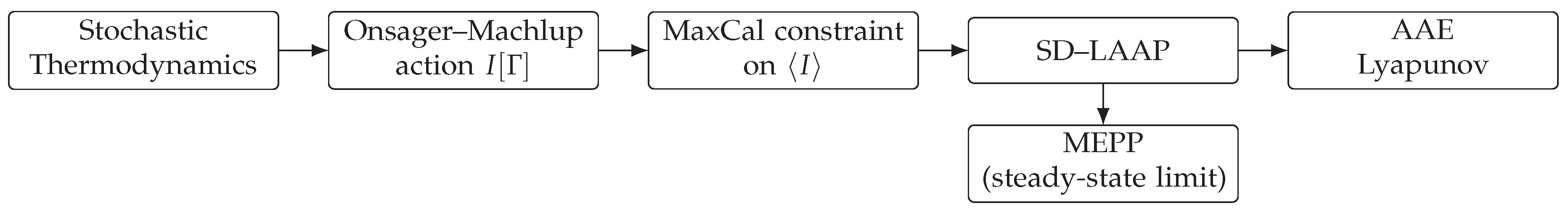

Table 1.
Examples of possible choices for the reference action unit in different systems.
| System | Event definition | Reference | Comments |
|---|---|---|---|
| Quantum system | One elementary transition | Natural universal quantum of action | |
| Chemical reaction | One molecule converted | Thermal energy–time product per reaction | |
| ATP synthase | One rotation or ATP hydrolysis | Empirically calibrated action per molecular cycle | |
| Ant foraging model | One complete trip nest → food → nest | Derived from observed energy and duration | |
| Brownian particle | One relaxation time | Product of thermal energy and correlation time |
Table 2.
Classification of dynamical regimes for action (SD–AAP) and AAE ().
| Regime | Principle | Interpretation | |||
|---|---|---|---|---|---|
| Self-organization | SD–DAAP | Lyapunov ↓; ; | |||
| Steady state/attractor | SD–LAAP | (NESS); constant | |||
| Disorganization | SD–IAAP | Lyapunov fails; ; |
Table 3.
Key terms and their precise meanings in this paper.
| Term | Precise Meaning in This Paper |
|---|---|
| Self-organization | Feedback-driven noise reduction satisfying and . |
| Feedback | Any internal process that modifies via the system’s own outputs. |
| Noise | The stochastic component of dynamics entering through variance . |
| Action | Path integral of a generalized Lagrangian including dissipative terms. |
| Average Action Efficiency (AAE) | : events per total action, dimensionless. |
| Lyapunov functional | Quantity that evolves monotonically under feedback (). |
Table 4.
Conceptual foundations of the stochastic–dissipative framework and their roles in this work [1,5,18,19,49].
| Concept / Theory | Definition or Essence | Role in This Work |
|---|---|---|
| Stochastic Thermodynamics | Describes fluctuating trajectories and entropy production under noise | Provides the formal foundation: corresponds to the Onsager–Machlup action used to compute path probabilities. |
| Maximum Caliber (MaxCal) | Maximizes path entropy subject to average constraints | Our path measure is the MaxCal solution under a constraint on average action . |
| MEPP | Steady states maximize entropy production under flux constraints | In our framework, MEPP emerges as a limiting inference case when and boundary fluxes are fixed; we do not assume it. |
| Lyapunov Functional | A quantity that decreases (or increases) monotonically under the dynamics | is proved to be a Lyapunov functional when ; its inverse measures efficiency growth. |
| Feedback-Controlled Systems | Dynamics with internal variables modifying noise or dissipation | Represented by the time-varying ; feedback strength controls the rate of self-organization. |
Disclaimer/Publisher’s Note: The statements, opinions and data contained in all publications are solely those of the individual author(s) and contributor(s) and not of MDPI and/or the editor(s). MDPI and/or the editor(s) disclaim responsibility for any injury to people or property resulting from any ideas, methods, instructions or products referred to in the content. |
© 2025 by the authors. Licensee MDPI, Basel, Switzerland. This article is an open access article distributed under the terms and conditions of the Creative Commons Attribution (CC BY) license (http://creativecommons.org/licenses/by/4.0/).
Copyright: This open access article is published under a Creative Commons CC BY 4.0 license, which permit the free download, distribution, and reuse, provided that the author and preprint are cited in any reuse.


