Submitted:
19 September 2025
Posted:
23 September 2025
Read the latest preprint version here
Abstract
We derive mass, gravity, and nuclear confinement from first principles through a spacetime mechanism where electromagnetic quantum vacuum fluctuations—originally derived from black-body radiation—induce metric perturbations that serve as a foundational source. Utilizing correlation functions, we demonstrate that highly coherent modes of zero-temperature black-body radiation undergo decoherence within the proton’s resonant cavity, producing its exact mass energy density. From Einstein’s field equations, we calculate the conversion factor of electromagnetic vacuum fluctuations into gravitational waves traveling through the proton’s cavity. We find that this converted energy is equivalent to the energy density of a Kerr-Newman solution at the proton’s reduced Compton wavelength, which defines a surface horizon. We compute the Hawking radiation and evaporation of this surface and find it equivalent to the proton’s rest mass. The evaporation lifetime far exceeds the observable universe’s age and satisfies experimental constraints. However, internal vacuum fluctuations within the proton cavity may provide a stabilizing source term equivalent to Hawking radiation energy, potentially affording extreme stability to the proton. Our formulation reduces to a Klein-Gordon equation on the metric perturbation that yields a confining Yukawa-like energy potential, demonstrating that both confining forces and gravitational forces emerge as consequences of metric perturbations generated by quantum electromagnetic fluctuations. This result aligns well with experimental measurements across multiple scales—from the color force to the residual strong force, and ultimately to gravitation. By computing both confining forces and gravity as emergent manifestations of vacuum fluctuations curving spacetime rather than separate fundamental interactions, we resolve Einstein and Rosen’s attempt to geometrize particles and forces at the quantum scale.
Keywords:
quantum vacuum fluctuations
; spacetime curvature
; gravitational waves
; mass generation
; Hawking radiation
; black hole horizons
; color confinement
; strong force unification
; Einstein field equations
Introduction
The origin of mass remains a central enigma in quantum field theories since the inception of modern particle physics [1,2]. The concept of mass remains profoundly unsettled within contemporary theoretical frameworks, with quantum chromodynamics (QCD), quantum electrodynamics (QED), and general relativity (GR) each conceptualizing "mass" through disparate mathematical and physical paradigms. In QCD, hadronic mass emerges predominantly from non-perturbative dynamics of the strong interaction, while the Higgs mechanism imparts bare masses to quarks via Yukawa couplings—accounting for only a negligible fraction approximately of total hadron mass [3,4,5]. In the context of QCD, the dominant contribution to proton rest mass instead arises from confinement energy, strong-interaction binding energy within gluon fields, and spontaneous chiral symmetry breaking [6,7,8,9,10]. Despite the combination of lattice QCD and the Higgs mechanism being recognized as the Standard Model explanation for hadronic masses, current lattice QCD simulations—incorporating gluon condensates and energy-momentum tensor form factors—reproduce proton mass values only by fitting parameters to match empirical parton distributions [11,12]. While numerically successful in reproducing hadron spectra [13,14,15], these form-factor approaches fail to fundamentally elucidate the physical origin of mass from first principles, unable to explain why the overwhelming majority of hadronic mass emerges from strong-interaction effects rather than the Higgs condensate. The intrinsically non-linear and non-perturbative nature of QCD renders a complete theoretical and analytical description of the proton’s mass and quark confinement mechanisms elusive, thus necessitating novel theoretical frameworks [16,17].
In QED, mass originates through renormalization procedures, wherein the divergent self-energy of charged point particles, such as the electron, undergoes absorption into a redefined physical mass parameter. Dirac initially identified this conceptual challenge in his seminal treatment of the electron’s self-interaction, which led to the formulation of an infinite "bare" mass shielded by vacuum polarization effects [18,19]. Contemporary QED formalism attributes the observed mass to the coupling between the electron and vacuum fluctuations of the electromagnetic field, which manifest in experimentally verified phenomena such as the Lamb shift and anomalous magnetic moment [20,21]. The zero-point energy of the quantized electromagnetic field contributes as a ubiquitous background, modifying fundamental particle properties via loop corrections; nevertheless, the renormalization scheme remains mathematically formal—effectively subtracting infinite quantities without providing substantive physical mechanisms underlying mass generation [22].
In general relativity, mass receives a fundamentally geometric definition through its influence on the spacetime metric tensor. According to Einstein’s field equations, mass-energy functions as the source term for spacetime curvature, with exact solutions such as the Schwarzschild metric explicitly establishing a mathematical correspondence between spherically symmetric mass distributions and resulting spacetime geometry [23,24]. Within this theoretical framework, the gravitational field becomes intrinsically encoded in the spacetime manifold structure, with inertial trajectories following geodesics defined by that curvature. While the equivalence principle successfully unifies gravitational and inertial mass concepts, it provides no explicit mechanism for mass generation; massive entities are postulated ab initio, and their gravitational influences are characterized through resultant metric curvature. Stated differently, GR presupposes the stress-energy tensor without specifying its microscopic structure, quantum origin, or the fundamental reason for mass-energy’s existence. This theoretical lacuna underscores the profound incompatibility between general relativity and quantum field theory in providing a coherent explanation for mass at the Planck scale. Considering the proton specifically, its mass effectively confines quarks through residual strong forces—yet interpreting these nuclear confining forces from a gravitational perspective would necessitate curvature magnitudes at femtometer scales that vastly exceed conventional expectations. Consequently, one might reformulate the inquiry, as Wilczek incisively proposed, not "why is gravity so weak?" but rather "why are hadronic masses so small?" [25]. This conceptual reframing illuminates that the conventional assumption of gravitational weakness may represent a fundamental mischaracterization; instead, a more profound physical mechanism might be actively screening vacuum energy with such remarkable efficiency that the observed hadronic mass appears inconsequentially small compared to the underlying vacuum energy density.
This fundamental tension between gravitational and quantum-mechanical conceptualizations of mass necessitates examination of unification attempts across theoretical physics. Efforts to reconcile these disparate theoretical frameworks have proven exceptionally challenging. Subsequent explorations, including Einstein and Rosen’s seminal work [26], employed a purely geometric conceptualization of particles as nonsingular wormhole solutions—representing particles as topological features rather than entities embedded within spacetime. Their approach described particles through "bridges" connecting two sheets of spacetime, avoiding singularities while unifying field and motion problems. In general relativity, these Einstein-Rosen bridges emerge from the same mathematical framework as black holes; a complete extension of the Schwarzschild solution demonstrate that a black hole from one perspective can be understood as a bridge to another region of spacetime, with the event horizon serving as the "throat." This geometrization approach to describing particles as spacetime structures, while mathematically elegant in classical general relativity, was ultimately abandoned primarily due to a significant scale discrepancy. Indeed, inserting the proton’s rest mass into the Schwarzschild solution yields a radius of meters— approximately times smaller than the Planck length and times smaller than the measured proton charge radius.
This geometric perspective experienced a remarkable renaissance through Susskind and Maldacena’s ER=EPR conjecture [27], which proposed a fundamental equivalence between Einstein-Rosen bridges (wormholes) and Einstein-Podolsky-Rosen entanglement. Their revolutionary insight suggested that quantum entanglement and geometric connectivity are different manifestations of the same underlying phenomenon. In this framework, Susskind and Maldacena viewed elementary particles as microscopic black holes, with quantum entanglement between particles corresponding to wormhole connections through spacetime. This approach offered a potential resolution to the scale problem that had previously derailed geometric particle models: rather than requiring classical Einstein-Rosen bridges at the Planck scale, the ER=EPR correspondence suggested that quantum mechanical effects at these scales naturally give rise to the geometric structures that manifest as particles. However, this framework remained largely conjectural, lacking the mathematical precision necessary to make testable predictions about particle interactions and hadronic mass.
Yet, the Einstein-Rosen’s approach contains a crucial insight that remained unrecognized for decades until now. The ratio between the measured proton radius and the calculated Schwarzschild radius yields precisely the fundamental constant , where represents the gravitational coupling constant—the ratio between the strong nuclear force and the gravitational force. This is no mere numerical coincidence: the calculation was revealing that the energy density concentration required at the proton scale to produce the observed confinement force is precisely .
This critical insight lies in reversing the conventional application of the Schwarzschild solution [?]. Rather than inserting the proton’s rest mass into to obtain an impossibly small radius, one should instead use the experimentally measured proton radius to calculate the requisite mass-energy that would generate a Schwarzschild radius of this size: . This inverted calculation yields , revealing that producing the observed strong confinement force requires a mass-energy density precisely times greater than the proton’s rest mass. This is not merely a numerical relationship but a fundamental physical insight: the ratio directly quantifies the screening of quantum vacuum energy density from Planck to nuclear scales.
Had this geometric relationship been recognized, it might have been realized that Einstein and Rosen’s approach was not failing but rather revealing the profound connection between spacetime geometry, vacuum energy density, and the hierarchy of forces—a connection that would require the full machinery of quantum field theory and an understanding of vacuum fluctuations to properly elucidate. Nevertheless, this pioneering work initiated a paradigm shift toward treating elementary particles as topological features of the spacetime manifold itself."
This geometric relationship between mass-energy density and force generation finds direct empirical validation in the nuclear mass defect phenomenon. When nucleons bind to form composite nuclei, the measured nuclear mass is systematically less than the sum of constituent nucleon masses: . This mass defect converts via Einstein’s mass-energy equivalence into the binding energy , which manifests as the residual strong force maintaining nuclear cohesion. For instance, the helium-4 nucleus exhibits a mass defect of approximately 0.03 atomic mass units, corresponding to a binding energy of 28.3 MeV—representing 0.75% of the total constituent mass transformed into confining force. This reveals that mass isn’t some immutable, unchanging quantity—it’s dynamic, convertible, and intimately connected to the forces and energies operating in nature. What we’re seeing is direct evidence that mass can transform into the very forces that bind matter together.
Recently, various researchers have unsuccessfully attempted to establish a consistent integration between general relativity and quantum chromodynamics [17,28]. String Theory and Loop Quantum Gravity (LQG) represent the most mathematically developed approaches of quantum gravity that seeks to unify quantum mechanics and general relativity. String Theory conceptualizes fundamental particles as one-dimensional vibrating strings, with gravity mediated by gravitons in a 10- or 11-dimensional spacetime [29], offering theoretical unification via the AdS/CFT correspondence [30], yet suffers from the landscape problem’s combinatorial explosion of possible vacuum states [31]. LQG provides a background-independent quantization of spacetime through spin networks, predicting a granular structure at the Planck scale [32,33], but encounters difficulties in recovering classical general relativity at macroscopic scales and lacks experimental validation [34]. Alternative formulations—including Causal Dynamical Triangulations, Asymptotic Safety approaches, and non-commutative geometry models—have similarly failed to resolve the fundamental theoretical incompatibilities [35]. The persistent limitations of these approaches—despite decades of intensive theoretical development—strongly suggests the necessity for fundamentally novel conceptual frameworks that transcend conventional quantum field theoretic and geometric paradigms, particularly in addressing the physical origin of mass and the nature of strong interactions at subnuclear scales.
Given these persistent challenges in unifying quantum theories with general relativity, we must reconsider the fundamental conceptualization of mass itself. Stepping back from the specialized treatments within individual theoretical frameworks, we observe that contemporary formulations of particle mass within the Standard Model framework necessitate confronting intrinsic infinities, manifesting either as the requirement for non-perturbative treatment of the QCD Lagrangian or as the introduction of divergent bare mass terms in QED renormalization schemes. Concomitantly, the framework of QED and subsequent advancements in quantum field theory established the concept of zero-point energy (ZPE)—a non-vanishing vacuum energy density persisting at absolute zero temperature [36,37]. Originating from Planck’s seminal resolution of the ultraviolet catastrophe in black-body radiation theory [38], ZPE introduced a fundamental term in quantum harmonic oscillator energy eigenvalues. Dirac, Pauli, Feynman, and other theoretical pioneers recognized that vacuum fluctuations necessitated by ZPE generate formal divergences when integrated across momentum space to arbitrarily short wavelengths [39]. These quantum vacuum fluctuations have subsequently received experimental validation through multiple independent phenomena, including the Lamb shift in hydrogen spectral lines [40], macroscopic Casimir force measurements between conducting plates [41,42], and spontaneous electron-positron pair creation [43]. These theoretical foundations and experimental confirmations necessitate a fundamental reconsideration of vacuum field ontology: whether quantum vacuum fluctuations function solely as regularization artifacts within renormalization procedures, or whether they constitute the primary causal mechanism underlying both inertial mass generation and the manifestation of nuclear interaction potentials.
In this paper, we propose that vacuum fluctuations constitute not merely a passive background medium for zero-point shielding, but rather the fundamental ontological substrate from which both inertial mass and spacetime curvature emerge as complementary manifestations. This proposition extends seminal contributions by Wheeler on quantum foam [44] and Sakharov’s mechanism of induced gravity [45,46], both of which establish theoretical frameworks wherein Planck-scale quantum processes translating the zero-point field fluctuations, are intrinsically and coherently related to local metric perturbations at that scale. Within this unified field-geometric paradigm, baryonic rest mass can be rigorously formulated as arising from coherent, collective excitation modes of the underlying vacuum field structure—specifically, the proton acts as a quantum-mechanical resonant cavity confining specific zero-point field eigenmodes exhibiting long-range collective phase correlation. The theoretical foundation for this mechanism draws further support from electromagnetic-gravitational coupling phenomena, including Yakov Zel’dovich’s investigation of electromagnetic-to-gravitational wave conversion [47] based on prior works [48,49], and Hawking’s analysis of primordial metric perturbations [50], which collectively indicate that sufficiently coherent electromagnetic field configurations generate spacetime curvature of sufficient magnitude to effectively confine energy within sub-femtometer volumes through purely geometric boundary conditions—thereby manifesting the phenomenological properties conventionally attributed to rest mass.
The foundational element of our theoretical framework connects the proton’s observed mass and strong nuclear forces with spacetime’s local geometry by examining how the proton’s core structure curves spacetime. Our formalism is grounded in Einstein’s field equations incorporating an explicitly defined electromagnetic stress-energy tensor constructed from zero-point field correlation functions at various length scales. Under weak-field perturbation analysis, the resulting covariant wave equations decompose into a system of coupled Klein-Gordon differential equations, each characterized by distinct eigenvalues corresponding to three fundamental length scales—Planckian, Comptonian, and hadronic—which solutions manifest precise exponential attenuation profiles mathematically isomorphic to the Yukawa potential that characterizes nuclear binding interactions [51]. This formulation elucidates how macroscopic gravitational "weakness" emerges naturally as a screened residual of the same underlying vacuum energy pressure that generates the effective "color-confining" force with explicit geometric origins within the proton’s internal structure.
The predictive capacity of the model extends beyond qualitative explanation, reproducing the empirical values of nucleon masses, quark pressure distributions, and the confining string tension derived from lattice QCD numerical simulations [13,14]. By reconceptualizing nuclear interactions, we replace the conventional interpretation of gauge bosons as abstract exchange particles with quantifiable metric fluctuations—physically real spacetime deformations generated by coherent electromagnetic vacuum oscillations that establish boundary conditions at critical screening horizons. Rather than relying on ad-hoc renormalization procedures that merely discard divergent terms, our approach provides a physically meaningful mechanism explaining how vacuum energy generates observable mass-energy while remaining gravitationally screened at larger scales. This unified framework—requiring no additional free parameters—demonstrates that the same zero-point fluctuations underlying fundamental QED processes simultaneously generate both hadronic matter’s self-gravitating structures and large-scale spacetime curvature—which manifests as what we classically interpret as forces, particularly here nuclear forces.
The manuscript is organized as follows: Section I presents a comprehensive overview of zero-point field theory within QFT. Section II addresses the vacuum energy density computation, its renormalization via Planck-scale cut-off, and the consequent relationship to Wheeler’s quantum foam topology. Section III derives the proton rest mass through correlation function analysis of vacuum energy fluctuations yielding the observed decoherence mechanisms manifest an apparent Hawking temperature. Section IV solves Einstein’s equations with quantum vacuum stress-energy. Section V analytically computes the proton rest mass as the Hawking radiation spectrum emanating from the proton’s core black hole structure identified in Section IV. Section VI examines the implications of these results for spacetime metric deformation through solutions to the coupled Klein-Gordon equation system, demonstrating that proton’s internal mass-energy structure induces observed phenomena including color confinement and residual strong nuclear interactions. The discussion Section broadens the theoretical framework to cosmological scales.
1. Origins and Development of Zero-Point Energy
1.1. Max-Planck and the Black Body Spectrum
The discovery of zero-point energy (ZPE) emerged from studies of black-body radiation, specifically through Max Planck’s efforts to resolve the ultraviolet catastrophe predicted by classical models. The initial framework was built on the Stefan-Boltzmann law
where is the Stefan-Boltzmann constant. From the classical model, Max Planck described atoms as harmonic oscillator cavities [36] and derived the radiated energy density (in ) in the frequency interval . By equating the absorption rate of an external electromagnetic energy by a black body and its emission rate he obtained the energy density spectrum
where is the total internal energy of the oscillator [38]. At the time, the challenge was the determination of the correct expression for .
Although the oscillator is typically visualized as a linear spring moving back and forth, it’s important to understand that this spring model is actually a one-dimensional projection of three-dimensional rotational motion. This 3D rotational perspective provides a more accurate representation of what occurs in real physical resonators, such as atoms.
After unsuccessful attempts by Rayleigh-Jeans () and Wien () [52]1. , Planck’s breakthrough came in 1901 with the law
However, a discrepancy in the internal energy expression led to Planck’s second attempt at resolving the ultraviolet catastrophe (1912), which introduced a crucial additional term to the internal energy expression
This second term, , represents what Max Planck coined the zero-point energy —a fundamental ground state energy persisting even at absolute zero temperature . Max Nernst later extended this concept to the vacuum field fluctuations, leading to the complete electromagnetic energy density spectrum
This groundbreaking formulation achieved a crucial unification between thermal radiation and vacuum energy, establishing zero-point energy (ZPE) as an intrinsic property of quantum systems [52]. While experimental validation would follow in subsequent years, this theoretical breakthrough carried its own challenge: the UV-catastrophe’s divergence was effectively replaced by a ground state energy density divergence. However, as we will explore in modern ZPE derivations, this divergence primarily manifests in coherent field modes—where phase correlations amplify energy fluctuations across the frequency spectrum—and only persists when analyses neglect the critical relationship between phase space scaling and spacetime metric structure.
1.2. Modern Derivation of ZPE in Free Electromagnetic Field
Modern quantum field theory describes electromagnetic quantum vacuum fluctuations energy density through correlation functions between field interference patterns. They are typically treated as a quantized electric field in the Coulomb gauge [37]
where , and characterizes the polarization of the plane wave. The normalization condition of over the quantization volume gives . The number of photons in the state emitted by quantum vacuum fluctuations follows the Bose-Einstein statistic for a gas of photons
The quantum operators follow the Hermitian property , which results in the decomposition of the electric field into positive and negative frequency components
The positive frequency component operates through annihilation operators , corresponding to photon absorption, while the negative frequency component employs creation operators , corresponding to photon emission [53] . The non-commutative behavior of these operators results in interference between positive and negative frequency components for each oscillator mode , observable in phase conjugation experiments [54].
In disordered systems, where quantum coherence is suppressed, this non-commutativity is set to zero, and the electromagnetic field energy density is given by the normally ordered correlation function
In a coherent system, positive (absorption/photon annihilation) and negative (emission/photon creation) frequencies can interfere resulting in a symmetrically ordered correlation function (see Appendix A)
where . When the field modes are sufficiently coherent (the characteristic time is very small, ), the electromagnetic energy density (in ) derived from the expectation value of the electric free field is
where is the Stefan-Boltzmann constant. The first term represents thermal radiation, while the second term represents the ZPE density
which displays a divergence at high frequencies. This is resolved by regularizing the field with a cut-off frequency as shown later in Section 2.2.
This formulation, developed through quantum electrodynamics (QED) and quantum field theory (QFT), establishes zero-point energy as a cornerstone of modern quantum mechanics—essential for explaining spontaneous particle creation, quantum interactions, and the critical renormalization procedures in both QED and quantum chromodynamics (QCD). The Standard Model, despite its celebrated predictive success in particle physics, remains fundamentally inadequate in its treatment of vacuum energies, offering merely computational workarounds rather than genuine physical insight. Its significant limitation lies in its inability to coherently integrate these energies with gravitational fields. This persistent incongruity underscores a fundamental gap in our current theoretical framework.
Attempts to renormalize infinities in quantum theory have profound implications for spacetime structure, culminating at black hole singularities where spacetime itself diverges to infinity according to general relativity. Hawking’s groundbreaking discovery of black hole radiation [55] catalyzed a fundamental crisis in physics—the information paradox—wherein quantum information appeared to be permanently lost when black holes evaporate, violating quantum mechanical unitarity. This contradiction spurred the development of the holographic principle, first proposed by ’t Hooft [56] and Susskind [57], and later formalized by Maldacena’s AdS/CFT correspondence [27], suggesting that gravitational systems can be completely described by quantum field theories of one lower dimension. Parallel explorations include Wheeler’s quantum foam [44], Hawking’s virtual micro-black holes [58], and the ER=EPR conjecture linking quantum entanglement with spacetime connectivity through Einstein-Rosen bridges. While these approaches primarily focus on resolving infinities and conservation laws in relativistic contexts, they often sidestep the fundamental renormalization issues in quantum mechanics. Nevertheless, applying spacetime formalisms at quantum scales may provide crucial physical insights into regularization and renormalization procedures, illuminating a path toward quantum gravity.
In the following, we will highlight how ZPE is a necessity in both theoretical approaches and experimental results analysis for consistency.
1.3. Zero-Point Energy: Mathematical Consistency and Its Role as a Source Term
The elucidation of the electromagnetic field in the vacuum state can be deduced from quantum mechanics. An electromagnetic field in vacuum is typically treated mathematically as a one dimensional harmonic oscillator, a model broadly used in quantum mechanics especially in perturbation theory [52]2. The generic quantum Hamiltonian for a harmonic oscillator is
with m the particle mass, the momentum operator, the position operator and the typical oscillator of force k frequency. Using Dirac’s creation and annihilation operators (, ) with the non-commutative rule , this becomes
yielding energy levels
with , the number of photons present in the mode .
The ground state () retains a non-zero energy , representing ZPE, the energy associated to quantum vacuum fluctuations. This zero-point energy serves as a crucial source term for the stability of matter, as demonstrated in the dipole model of the atom which takes into account the radiation reaction field (in the small-damping approximation ) and the vacuum fluctuation source is
with and the natural frequency of the system. Without quantum vacuum fluctuations (), the dipole would collapse as
In fact, the quantum vacuum fluctuations act as a source term necessary to the stability of matter, counterbalancing the radiative damping of the dipole. Including the source term (), the solution becomes
This source term maintains both the stability of matter and the fundamental non-commutative relationship (see [52], p 53), from which emerges the uncertainty principle
Zero-point energy is not merely a mathematical artifact but a physical necessity for the stability of quantum systems and the foundation of quantum mechanical principles [52]. Without this irreducible ground state energy, quantum systems would collapse into their classical counterparts, undermining the entire framework of quantum mechanics. Quantum vacuum fluctuations manifest as perpetual fluctuations in quantum fields—even at absolute zero temperature—preventing particles from simultaneously occupying precise positions and momenta.
These vacuum fluctuations fundamentally maintain the non-commutativity of conjugate operators , establishing the algebraic structure from which the Heisenberg uncertainty principle naturally emerges. This causal relationship is frequently misunderstood: contrary to what is commonly presented, the uncertainty principle is a consequence of ZPE, not its source [52]. The primacy of ZPE in quantum theory is further evidenced by phenomena such as the Casimir effect, Lamb shift, and spontaneous emission, where measurable physical effects arise directly from vacuum field fluctuations and cannot be attributed to uncertainty principles— defining unambiguous experimental confirmation of ZPE’s ontological status beyond mathematical formalism (see Appendix B for extensive list of experimental validation of ZPE).
Furthermore, quantum vacuum fluctuations provide the mechanism through which virtual particle-antiparticle pairs continuously emerge from and return to the vacuum, creating a dynamic substructure that permeates seemingly empty space. This quantum "foam" not only mediates fundamental forces through virtual particle exchange but also reveals the vacuum as an active, energy-laden medium rather than an inert void—establishing ZPE as perhaps the most ubiquitous yet underappreciated physical reality in our universe.
The zero-point energy’s treatment within quantum field theories —particularly in Quantum Electrodynamics (QED) and Quantum Chromodynamics (QCD) —presents fundamental problems for mass generation mechanisms. Renormalization techniques, while computationally effective, have raised profound mathematical concerns among quantum theory’s founders. Dirac (1975) challenged the mathematical legitimacy of these approaches, asserting that "Sensible mathematics involves disregarding a quantity when it is small – not neglecting it just because it is infinitely great and you do not want it!" [39]3 This critique directly questions how QED and QCD handle infinite quantities when calculating particle masses. Feynman (1985), despite his pivotal role in developing QED, remained skeptical of its mathematical foundation, describing renormalization as a "dippy process" and "hocus-pocus" that has "prevented us from proving that the theory of quantum electrodynamics is mathematically self-consistent," ultimately suspecting that "renormalization is not mathematically legitimate." [59]4 These criticisms from two Nobel laureates highlight how the treatment of zero-point energy affects our understanding of mass generation in fundamental physics, suggesting that current frameworks may require significant theoretical revision.
In the Sections below, we explore the relationship of ZPE and the associated vacuum fluctuations to the structure of spacetime, its physical relevance and role in experimental work.
2. Quantum Electromagnetic Vacuum Fluctuations and Its Energy Density
2.1. Quantum Vacuum Energy Density
In this Section, we examine how quantum vacuum fluctuations shape spacetime structure and contributes to mass definition. Having established ZPE’s theoretical foundations and experimental validation, we now derive its total vacuum energy density. Electromagnetic quantum vacuum energy density emerges exclusively in coherent space (cf. Equations (12), (13) and Appendix A), arising from the sum of elementary spherical harmonic oscillators with ground state energy across all possible field modes . For a three-dimensional spherical oscillator—functioning as a resonant cavity—the ground state energy of the three-dimensional Hamiltonian for rotational oscillations is given by
and the vacuum energy density for a continuous mode distribution is (see Appendix C)
where represents the number of modes between and in volume V. When an infinite number of modes is permitted (i.e., ), the vacuum density diverges. Thus, the vacuum energy divergence occurs when an infinite amount of scales is considered underlying the possible fractal nature of spacetime at the quantum scale defined by the Planck scale, which is found as well in cosmology at the horizon of black holes where the entropy is computed as the holographic principle [56,60]. Furthermore, spacetime vacuum that appears flat at a large scale is in fact extremely energetic and fluctuating at the small scale of the quantum world.
Einstein’s general relativity equations establish that all energy-momentum distributions fundamentally determine spacetime geometry, manifesting as gravitational phenomena. This principle suggests that the immense energy fluctuations inherent in the quantum vacuum should generate profoundly curved, topologically complex spacetime geometries with significant gravitational consequences, which we later connect to nuclear confinement mechanisms (see Section 7).
Wheeler’s seminal work on Quantum Geometrodynamics [44] demonstrates that virtual particle-antiparticle pairs, perpetually emerging from and returning to the vacuum at Planck scales ( m), induce continuous, dynamic distortions in spacetime fabric. These quantum vacuum fluctuations operate with such intensity that they fundamentally undermine the conventional notion of spacetime as a smooth, deterministic continuum with well-defined geometric properties.
Rather than a featureless void, Wheeler proposes conceptualizing spacetime as "quantum foam"—a probabilistic superposition of all possible geometric configurations and topological connectivities that only approximates classical smoothness when observed at scales significantly larger than the Planck length. This revolutionary framework suggests that spacetime itself emerges as a statistical phenomenon from underlying quantum fluctuations, reconciling the apparent contradiction between quantum mechanics’ probabilistic nature and general relativity’s deterministic geometry.
Wheeler illustrates this concept by comparing quantum foam to an ocean surface. From a great distance, the ocean appears perfectly flat, showing no measurable energy. Closer inspection reveals waves with measurable energy, and further magnification exposes breaking waves and foam formation. Each observation scale corresponds to a distinct energy level, that is to say in the case of spacetime, a mass.
2.2. Natural Cut-Off at the Quantum Scale
In his seminal work, Wheeler provided compelling evidence for both this cut-off and the existence of quantum foam by determining the precise length scale at which spacetime metric fluctuations emerge in response to vacuum electromagnetic fluctuations [44]. His analysis centered on the phase of the Feynman-Huygens equation, combining an Einstein-Hilbert action with an electromagnetic free field. The exponent phase in this equation is given by
where S represents the total action, A denotes the vector potential, and represents the spacetime metric. Within a four-dimensional spacetime region , the phase variation in the path integral formulation—arising from both metric perturbations and electromagnetic fluctuations in the vector potential —can be expressed as (see Appendix D and [44])
Field variations in this region contribute to path histories when phase variations are sufficiently small to generate constructive interference, specifically when . According to Einstein’s Field Equation, electromagnetic vacuum fluctuations induce spacetime curvature, resulting in a metric variation
This leads to electromagnetic and gravitational phases of equivalent magnitude
Consequently, the characteristic metric and electromagnetic field energy density fluctuations scale as and . Since metric fluctuations reach their maximum at , the characteristic length L of these fluctuations approximates the Planck length
Furthermore, the electromagnetic field oscillators at the Planck length scale carry energy on the order of the Planck mass
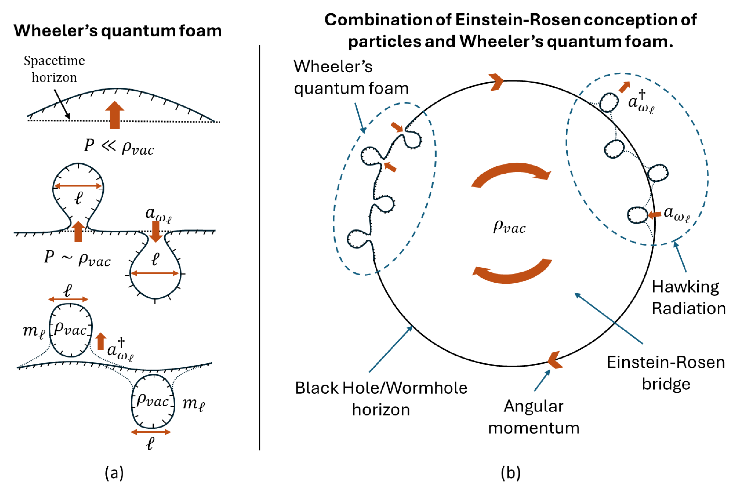
Wheeler’s investigation revealed that electromagnetic vacuum fluctuations create gravitational responses resulting in a "quantum foam" at the Planck length scale ℓ, where metric fluctuations directly and coherently respond to quantum vacuum fluctuations. At this scale, spacetime curvature fluctuations form virtual wormholes with Planck-scale properties: charge , mass , and energy related to zero-point energy. These fluctuations cause spacetime to pinch into self-gravitating entities (Figure 1.a).
Wheeler’s spacetime bubble theory builds upon Einstein and Rosen’s 1935 work while incorporating quantum mechanics. Unlike Einstein-Rosen’s stable bridges representing permanent particles, Wheeler’s quantum geometrodynamics introduced quantum uncertainty, proposing that spacetime undergoes continuous topological fluctuations at the Planck scale. In this framework, fundamental particles emerge from coherent disturbances in these fluctuations, as transient micro-wormholes form and annihilate. Wheeler thus preserved Einstein’s geometric vision while adding the quantum principles absent from the original Einstein-Rosen model.
Figure 1.
(a) Elementary spacetime nucleation producing ’virtual’ particles from spacetime pinches due to electromagnetic quantum vacuum fluctuations at the Planck scale and characterizing the annihilation and creation operators. The resulting Planck scale ’voxels’ have a Planck mass . (b) Combination of Einstein-Rosen bridge (or wormhole) and Wheeler’s quantum foam. The creation-annihilation processes at the black hole/wormhole horizon screen the internal vacuum energy density which coherency is induced by the angular momentum (or circulation) in the Planck plasma.
Through another analysis of the relationship between general relativity and quantum mechanics, we find a similar minimum wavelength scale to determine the lower boundary condition of the energy at which spacetime will nucleate. This scale emerges when we combine spacetime dynamics with the Heisenberg uncertainty principle arising from zero-point energy (ZPE). When vacuum fluctuations behave coherently, they induce mass-energy concentrations which curve spacetime and result in angular momentum in spacetime, suggesting that quantum foam structures may resemble microscopic Kerr-Newman vortices (see Section 4.2). This framework establishes a regularization cut-off and yields a minimal angular momentum value for an extremal spacetime vortex, characterized by momentum p, energy , and radius R. Considering Wheeler’s approach and utilizing the uncertainty principle, we have
where represents the vortex radius and denotes the relativistic momentum flow (). Thus, the minimal angular momentum is and it obeys the condition . Such structure emerges in the spacetime metric, producing quantum foam at the critical Schwarzschild limit where . By resolving these two conditions from quantum mechanics and general relativity, we obtain a cut-off condition that corresponds to the unifying energy of the Planck scale
with and ℓ representing the Planck mass and length respectively. These Planck units define a fundamental minimum scale in spacetime structure, which physicists typically choose as a limiting case when studying black hole singularities and early universe cosmology [55].
2.3. Consequences of the Planck Length Cut-Off
We have used two different approaches to describe the relationship between electromagnetic vacuum fluctuations and spacetime curvature resulting in a natural cut-off value of the spacetime structure at the Planck scale. Returning to Equation (27) and renormalizing with an oscillator of characteristic diameter of the order of the Planck length ℓ, we obtain a cut-off pulsation
and a finite vacuum energy density expressed as
which corresponds to the Planck density, typically expressed as , multiplied by the geometric factor . This geometric factor arises because the universal oscillator is spherical rather than cubic. The geometry of space becomes particularly important when we examine the fundamental spacetime fabric voxels and calculate black hole entropy in the context of Hawking radiation (see Section 5). Therefore, examining equation (38), the vacuum fluctuations energy density can be computed by the aggregate of elementary spacetime voxels of mass in a volume V
where represents a single voxel’s volume. These fundamental spacetime voxels can be mathematically characterized as spherical cavity harmonic oscillators—precisely the quantum mechanical systems that underpin Planck’s blackbody radiation law. Each oscillator possesses a minimum ground state energy at absolute zero temperature, consistent with the zero-point energy predicted by quantum field theory
Importantly, these voxels exhibit a plasma-like fluid structure analogous to quark-gluon plasma (QGP) observed in high-energy physics experiments [61,62]. This non-trivial vacuum architecture generates coherence within quantum vacuum fluctuations through plasma fluid vorticity mechanisms, as proposed in modified hydrodynamic models of quantum vacuum [63]. The resulting topological structures can be described using techniques from magneto-hydrodynamics, where coherent vortical excitations emerge naturally from the underlying field equations [64].
The quantum vacuum structure described above—with its spherical oscillators and plasma-like vortical dynamics—provides a microscopic foundation for macroscopic gravitational phenomena. To bridge these scales coherently, we can formalize the fundamental relationship between quantum vacuum fluctuations and general relativity by expressing the Schwarzschild metric using Planck units ( metric signature convention)
as well as the general form of the Einstein Field Equations
These equations establish Planck units and zero-point energy as natural normalization factors in general relativity. Analyzing the Einstein Field Equations in dimensionless form confirms the Planck scale as fundamental, with ZPE density generating spacetime curvature (Ricci scalar R) on the order of the Planck length , consistent with our earlier cut-off. Just as a soap bubble balanced by internal pressure and surface tension, a stable Schwarzschild black hole represents perfect equilibrium where outward repulsive pressure exactly counterbalances the inward pull of spacetime elasticity .
Both mathematical approaches—Wheeler’s path integral formulation and our analysis combining uncertainty principles with general relativity—confirm the Planck scale as a fundamental physical threshold, not merely a mathematical construct. This natural regularization cut-off resolves the divergence in quantum vacuum energy density while establishing a dimensional threshold for physical equations. At this scale, spacetime transitions from a continuous manifold to a dynamic quantum foam made of Planck scale wormholes and topological fluctuations. Expanding Wheeler’s ocean analogy, just as the surface of a fluid, spacetime curvature appears continuous at macroscopic scales but fragments into discrete structures microscopically. At ultra-small dimensions, extreme spacetime curvature folds upon itself, creating quantized geometric elements. This self-enclosure provides a coherent explanation for the transition from continuous differential geometry of general relativity to the inherently discrete nature of quantum spacetime. Our paper develops two complementary frameworks: the continuous approach to spacetime metric in general relativity, and the discrete perspective resulting from the electromagnetic quantum vacuum fluctuations curving spacetime at the microscale (see Section 4.1, Section 5.3 and Section 7.1).
3. The Origin of Mass as Coherent Modes of Quantum Vacuum Fluctuations at the Hadronic Scale
3.1. Electromagnetic Vacuum Fluctuations Correlation Functions in the Temperature-Independent Regime
Our analysis thus far has established that ZPE density—which emerges from coherent modes of electromagnetic fields radiated by a zero-temperature black body—exhibits two critical behaviors: it either diverges when correlation time vanishes (, see Section 1.2) or it approaches the very high Planck energy density when regulated by a Planck-scale cutoff (corresponding to correlation time ). This demonstrates that the system’s energy density is fundamentally governed by the correlation time , which characterizes the coherence intervals of constructive quantum interference patterns. We now extend these same correlation functions and analytical frameworks to explore analogous quantum vacuum phenomena at the vastly larger hadronic scale (some 20 orders of magnitude larger), where similar coherent structures emerge with profound implications for our understanding of mass and nuclear forces generation. To investigate the decoherence process of ZPE density at macroscopic scales, we analyze the system energy density using first-order correlation functions for a black-body radiation field. We consider a characteristic correlation time that delineates the decoherence scale of electromagnetic vacuum fluctuations within the low-temperature regime where as a first approximation (temperature’s impact will be addressed later in Section 3.3). Under these conditions, the correlation functions for black body radiation reduce to their temperature-independent terms (detailed in Appendix A, Equation (A13))
where is the Planck time and the ZPE density at the Planck cut-off. Remarkably, when we consider a significant change of scale, or orders of magnitude, and we implement the characteristic time of the proton defined by
where is the proton RMS charge radius, which is as well consistent with the characteristic time of the strong nuclear force typically given by the meson lifetime (), we obtain the energy density of that scale resulting from the decoherence of considering the creation and annihilation cycle reducing by a factor of 2
Thus, the corresponding energy for that scale resulting from the coherent behaviour of the quantum vacuum fluctuations in the volume of a proton is
The uncertainty range translates the uncertainty in measuring precisely the proton charge radius. This profound, non-trivial result demonstrates how our theoretical framework precisely derives an energy range in which the experimentally measured rest mass of the proton falls (). Our model establishes a direct relationship between the Planck scale vacuum energy density and the proton’s rest mass through a precisely calibrated decoherence or screening mechanism. The quantum field theoretical framework we derived reveals how Planck-scale vacuum fluctuations undergo systematic screening via coherent quantum processes, ultimately manifesting as the observed proton mass.
This screening phenomenon emerges from our analysis of the dynamical equilibrium between creation and annihilation processes of virtual particle-antiparticle pairs within a cavity of proton-scale characteristic dimension. The mechanism effectively converts a precisely determined fraction of electromagnetic vacuum energy into gravitational potential energy. This transduction operates through vacuum fluctuations decoherence that is analogous to, yet distinct from, symmetry-breaking principles observed at the quantum chromodynamic scale. Section 4 computes the comprehensive mathematical formalism of this process, including explicit derivations of the coupling constants that govern the screening mechanism.
This theoretical framework naturally extends to a complementary interpretation where the proton functions as a quantum electrodynamic resonant cavity with characteristic length . In this model, the screening mechanism manifests as a modified Casimir effect, where the quantum vacuum pressure exerted on the cavity boundaries generates both the proton’s rest mass and its confining force. The Casimir pressure, expressed generically as where a is the cavity’s characteristic length, precisely matches our derived proton rest mass energy density with the geometric factor characterizing our specific boundary conditions. When quantified, the resulting confining Casimir force can be estimated as
This value aligns remarkably with the measured magnitude of the strong nuclear interaction (see Section 7 for in-depth analysis of forces), providing compelling evidence that hadronic mass and nuclear binding forces share a common origin in quantum vacuum dynamics. This unification reveals a profound connection: both nuclear confinement and mass emerge from quantum vacuum fluctuation dynamics through a Casimir-like effect. Recent experimental measurements of proton pressure distributions [65,66] corroborate this framework, demonstrating that the binding pressure force is generated by quantum vacuum fluctuations as our model predicts.
3.2. Effective Radius and the Charge Radius ’Puzzle’
Our analysis of the correlation functions reveals a direct relationship between the proton’s charge radius and its rest mass , which links to its reduced Compton wavelength . Due to the large uncertainty on the charge radius measurement, this result cannot meet the precision of the experimentally measured proton rest mass. However, as this equation was already obtained geometrically by one of us utilizing Planck units [67], we deduce that this relationship is exact and can be expressed concisely as:
The reduced Compton wavelength emerges as a fundamental parameter in our theoretical framework for several reasons:
- 1.
-
It marks the quantum-classical boundary through two mechanisms:
- At distances approaching , Heisenberg’s uncertainty principle shows momentum uncertainty becomes , making relativistic effects and particle-antiparticle pair creation energetically possible
- Solutions to the relativistic Klein-Gordon equation diverge from the non-relativistic Schrödinger approximation at
- 2.
- It establishes the characteristic scale at which vacuum fluctuations effectively couple to the proton’s mass-energy structure
- 3.
- It governs the exponential decay rate of virtual mesons mediating the nuclear force, as Hideki Yukawa demonstrated [51], where the potential follows
Most significantly, our derivation shows that defines the radius at which vacuum energy screening transitions from quantum-dominated to classically observable effects. The relationship reveals a geometric efficiency factor in how vacuum energy configures into observable mass. This parameter is essential in quantifying the screening mechanisms explored in Section 4.1, Section 5 and Section 7 where we demonstrate how vacuum fluctuations generate both the proton’s mass and the nuclear binding force.
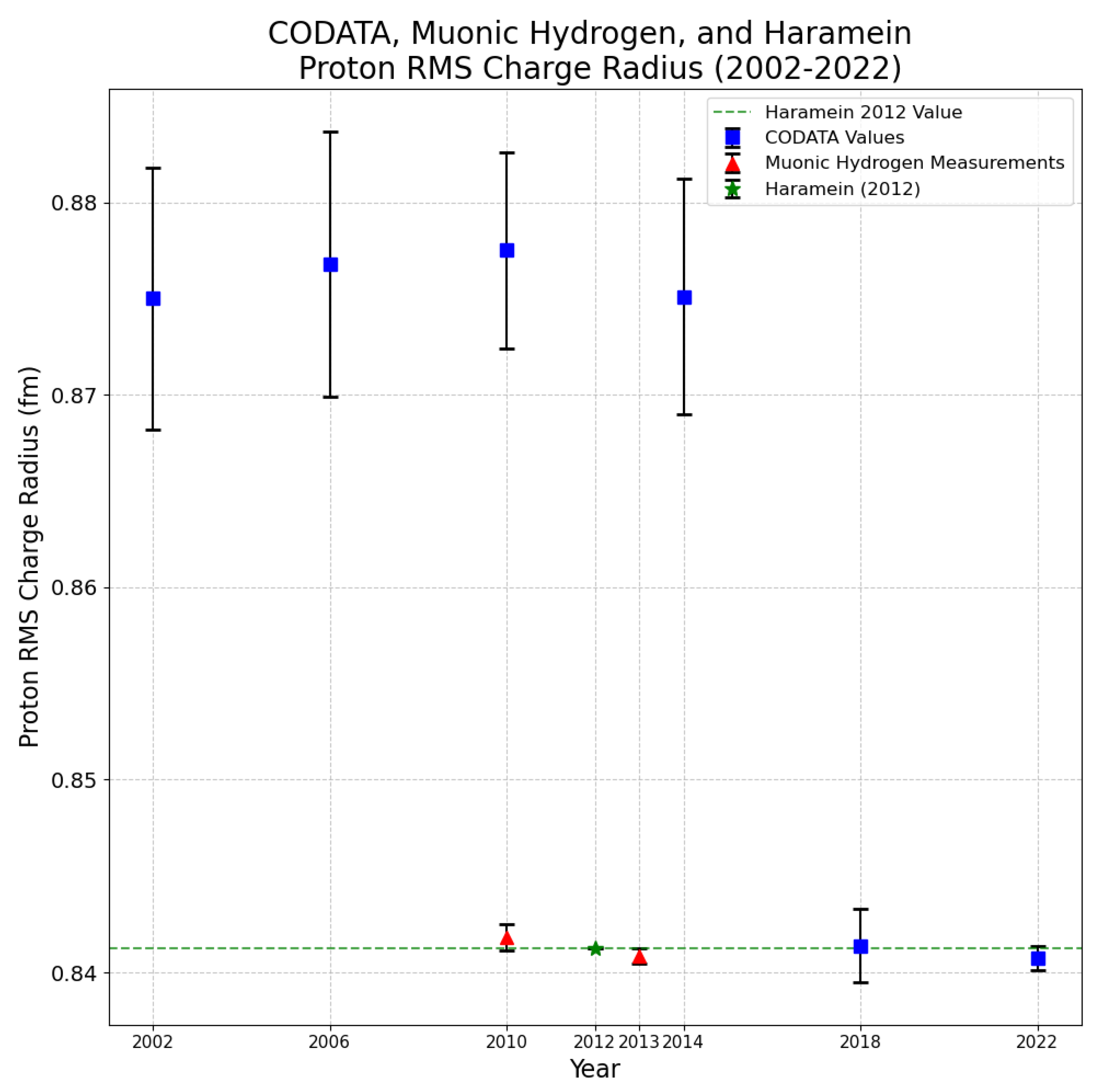
These results connect to the ongoing discussion regarding the proton radius puzzle (Figure 2). The proton charge radius is defined by the slope of the proton charge form factor at zero momentum transfer. In 2010, muonic hydrogen spectroscopy measurements revealed a ’small’ radius of , significantly different from the previously accepted ’large’ radius of obtained via electron-proton scattering and hydrogen spectroscopy. The holographic mass approach, proposed in 2012, relates the proton’s rest mass to its charge radius through the same equation (green star on Figure 2 and [67]). This framework, incorporating vacuum electromagnetic fluctuations and phase coherence, yielded a radius value consistent with the smaller measurement before its widespread acceptance (Figure 2) with six digits greater precision thanks to the high precision on the proton rest mass measurement.
From 2017 onward, refined electron-proton scattering experiments with smaller momentum transfer corroborated the ’small’ radius measurement. Reanalysis of previous experimental data using models that incorporate Zero Point Energy (ZPE) contributions brought older measurements into alignment with this value. The Codata 2022 recommended value of reflects this convergence, supporting theoretical frameworks that predicted values in this range through vacuum fluctuation approaches.
Figure 2.
Historical evolution of the CODATA values for charge radius measurement originally based on electron scattering. The fundamental change in CODATA 2018 was based on experiments starting in 2010 of more precise muonic measurements and re-analysis of the previous electron scattering measurements [68?]. This graph shows how the geometrical and holographic approach of [69] (green star prediction) recovered in this paper from the correlation functions analysis at the proton scale predicts the most recent and precise measurement of the proton charge radius.
3.3. Temperature Emergence from Quantum Vacuum Decoherence
In our prior analysis of the proton rest mass derived from black body electromagnetic field correlations over the proton’s characteristic time , we initially neglected temperature-dependent terms to establish a first-order approximation of the decoherence process. Given the profound reduction—approximately 80 orders of magnitude—from quantum vacuum energy density () to proton rest mass-energy density (), a more complete model requires examining the fundamental relationship between coherence time and temperature T generated by quantum vacuum fluctuations within the Planck Plasma. We propose that decoherence processes must correlate with temperature increases, analogous to free mean path dynamics in gas theory, which can be expressed mathematically as .
By incorporating both temperature-dependent and temperature-independent terms in the correlation function yielding Equation (12), we can determine the thermodynamic point at which the total electromagnetic field energy density matches the proton’s rest mass density. This relationship is expressed formally as
where and .
The solution to this equation reveals two distinct solutions: . The first solution corresponds to the zero-temperature limit (), which is physically interpreted as a vanishing coherence time () leading to the previously identified energy density divergence. The second and non-trivial solution, when combined with our established relation , yields
This result carries profound implications: our model demonstrates that when both coherence time and finite-temperature effects are properly accounted for in quantum vacuum fluctuations, the derived temperature exactly matches the Hawking temperature for a black hole whose radius equals the proton’s reduced Compton wavelength. This remarkable correspondence establishes a deep connection between quantum field thermodynamics and spacetime geometry at the hadronic scale—a relationship that will be explored in the following Section.
The emergence of this Hawking-equivalent temperature indicates a fundamental mechanism wherein collective, coherent electromagnetic quantum vacuum fluctuations directly influence spacetime geometry, inducing Bogoliubov transformations between flat and curved spacetime field operators: . These mathematical transformations represent the vacuum state transition , wherein the curved spacetime vacuum appears to a flat-space observer as a thermal state populated with correlated particle-antiparticle pairs. This precisely generates thermal radiation with temperature proportional to spacetime curvature at the effective horizon—a mechanism we will examine extensively in Section 5.
From an alternative perspective, this phenomenon manifests as a generalized Unruh effect, in which an observer undergoing uniform acceleration a through vacuum detects thermal radiation at temperature , while an inertial observer registers only vacuum fluctuations. In our theoretical framework, the coherent collective behavior of quantum electromagnetic fields produces measurable geodesic deviation (quantifiable as proper acceleration), causing neighboring worldlines to experience relative acceleration. This acceleration-induced horizon establishes an observer-dependent thermodynamic boundary. In the forthcoming Section, we will demonstrate quantitatively how the collective coherent dynamics of the Planck plasma generates sufficient spacetime curvature to produce the characteristic temperature .
4. From Quantum Vacuum Fluctuations to Gravitational Field in General Relativity
The quantum vacuum’s microscopic fluctuations play a crucial role in shaping the geometry of spacetime through their collective behavior. These fluctuations manifest as minute disturbances in the quantum fields permeating all of space, creating a dynamic fabric that simultaneously responds to and influences gravitational forces. In his groundbreaking 1967 work, physicist Andrei Sakharov proposed a microscopic foundation for gravitation arising from quantum vacuum fluctuations. Sakharov introduced the concept of "metric elasticity of space," incorporating the Planck length cut-off to establish a direct equivalence between electromagnetic vacuum fluctuations and the gravitational constant G [45].
with , a geometrical constant on the order of unity and is the sum of all modes of the electromagnetic vacuum fluctuations. Considering the Planck length cut-off, according to Sakharov’s definition, the gravitational force results directly from the energy density of the fluctuations in the quantum foam determined by the scale of the smallest oscillator [70]5. Here, the electromagnetic vacuum fluctuations are the source of spacetime elasticity generating the gravitational constant. However, the mechanism under which the microstates of the quantum vacuum electromagnetic field is converted to a gravitational component is undefined.
By treating the microstates of electromagnetic vacuum fluctuations as the fundamental building blocks of spacetime, we can demonstrate how classical gravity emerges from quantum mechanics. This approach creates a natural bridge between quantum field theory and general relativity, where classical geometry emerges as a collective behavior arising from quantum vacuum states.
4.1. First Screening : Electromagnetic Vacuum Fluctuations to Gravitational Wave Generation
In 1973, physicist Yakov Zel’dovich, building upon earlier work [48,49,71], characterized the conversion of electromagnetic waves into gravitational waves when propagating through a strong magnetic field [47]. Zel’dovich demonstrated that an electromagnetic wave with energy density traveling through a magnetic field H partially transfers its energy into gravitational energy. This gravitational energy flux along the propagation direction (specifically, along the r-direction in spherical coordinates) can be quantified using the Landau-Lifschitz pseudo-tensor component . Although this mechanism represents a classical effect derived directly from Einstein’s field equations (see Appendix E), it exhibits characteristics analogous to a phase transition, wherein an extremely coherent electromagnetic field at the Planck scale undergoes an abrupt transformation to a lower coherence, curving spacetime at the hadronic scale.
While Zel’dovich described this mechanism as a ’conversion’ between electromagnetic and gravitational waves, it is crucial to understand that the electromagnetic wave generates a non-zero stress-energy tensor that produces gravitational curvature through Einstein’s Field Equations. The amount of gravitational curvature depends on the energy density of the electromagnetic wave, which in our case is related to the Planck plasma coherence or phase in that region of space. At sufficiently high energy densities to overcome spacetime elasticity, the electromagnetic field creates a gravitational field strong enough to confine most of the electromagnetic energy within a bounded region, i.e. a bubble is formed.
This self-confinement mechanism establishes a direct equivalence between the electromagnetic and gravitational components, both manifestations of the same underlying physical reality, rather than separate phenomena. The gravitational and electromagnetic descriptions represent complementary physical manifestations of a unified mechanism, such that the term ’conversion’ here describes how electromagnetic waves decohere in the presence of their own gravitational fields, with most energy remaining trapped in electromagnetic form while a portion manifests as gravitational radiation.
In this work, we model proton mass-energy density as the manifestation of quantum electromagnetic vacuum fluctuations’ collective behavior (Planck plasma flow) at the Planck scale producing gravitational energy flux at the proton scale. The Planck plasma flow can be conceptualized as spacetime voxels carrying a fundamental Planck charge and exhibiting a toroidal flow (see Figure 3.b). This flow generates vorticity and ensures high coherency () within the proton’s core. This configuration enables the production of an incident electromagnetic wave radiating radially from the center with energy density , passing through the static magnetic field H produced by the circulation of spacetime voxels at the proton’s core surface, identified at its reduced Compton wavelength . Due to the extremely high quantum vacuum energy density, which vastly exceeds the Schwarzschild condition, the resulting electromagnetic field is sufficiently strong to curve spacetime, generating a gravitational force that characterizes the proton’s mass-energy. Utilizing the formalism on which Zel’dovich’s analysis was built upon [48,49], we evaluate the corresponding gravitational component by computing the Landau-Lifschitz pseudo-tensor in the weak field approximation for Einstein’s field equations, which gives the energy flux per unit time radiated by the proton’s core surface
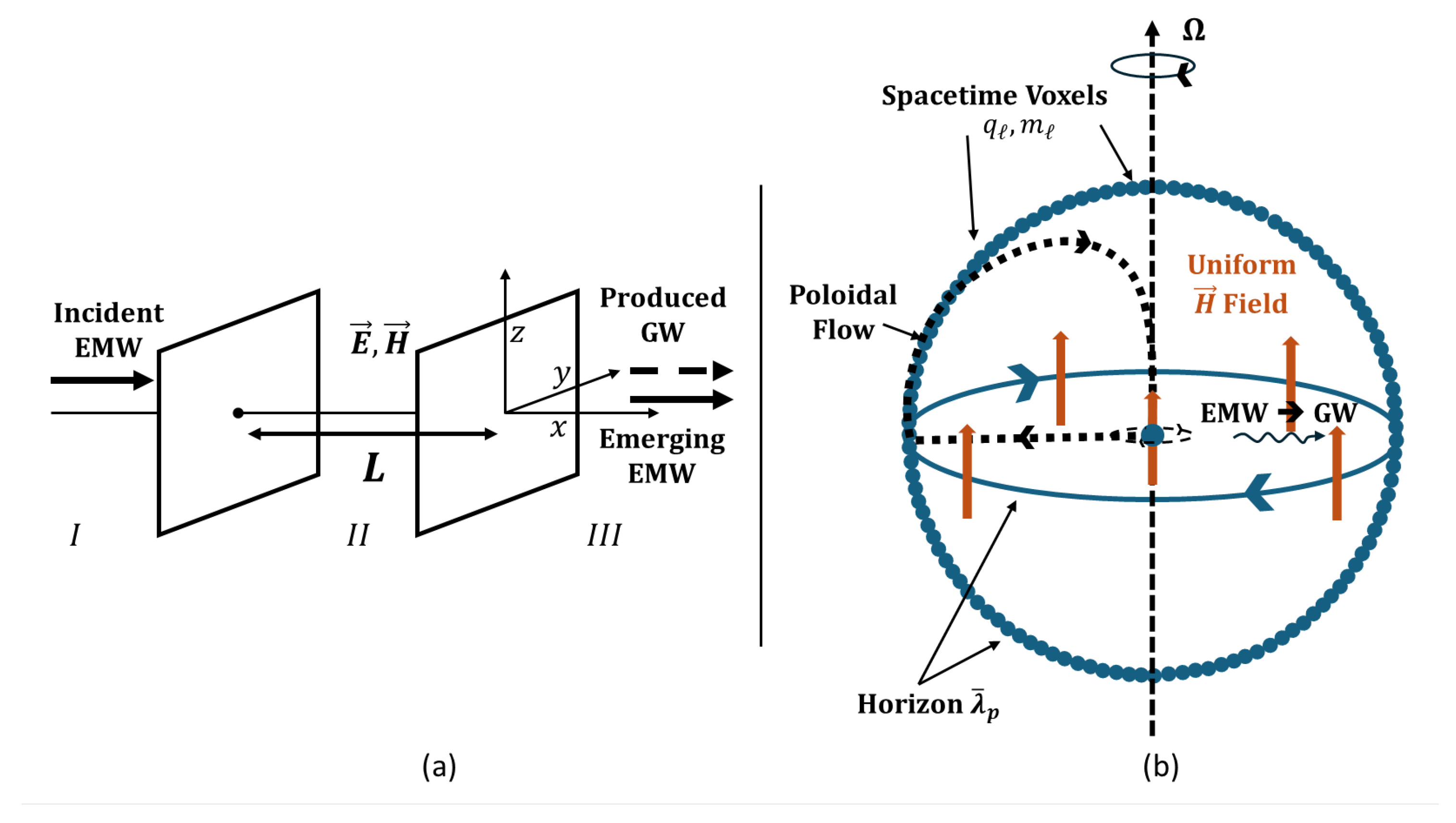
Figure 3.
(a) Initial work from Boccaletti et al. investigating the conversion efficiency of electromagnetic waves (EMW) into gravitational waves (GW) as they propagate through a strong static electromagnetic field () over distance L (adapted from [49]). (b) Our proposed model illustrating the EMW-to-GW conversion mechanism at the hadronic scale. Here, an EMW generated by a spacetime voxel undergoes conversion to a GW. The magnetic field strength is produced by a spherical shell of Planck charge , which forms through the circulation of spacetime voxels orbiting at the modified Compton wavelength .
where is vacuum permeability and is the path length of the electromagnetic wave through the magnetic field (see Appendix E for the detailed derivation).
We compute the proton’s internal magnetic field at its reduced Compton wavelength through the coherent flow of Planck plasma quantum vacuum fluctuations. As a first-order approximation, these voxels collectively behave as an outer charged rotating spherical shell, thereby generating a constant magnetic field vector that aligns parallel to the rotation axis (here the z-axis). The magnitude of this intrinsic magnetic field can be expressed as
where is the pulsation of the toroidal circulation undergoing four poloidal circulations in one toroidal rotation. With path length , the energy transfer from electromagnetic vacuum fluctuations to the gravitational component can be computed as
Thus, the total gravitational wave energy radiated at the surface over a characteristic time is
which is equivalent to a gravitational energy density within the enclosed volume
We can now identify the conversion coefficient of the electromagnetic wave energy density converting to a gravitational wave travelling through the proton’s core as
This extremely small gravitational conversion coefficient of the electromagnetic vacuum density represents a significant screening of the energy density available within the proton at that scale—thus the weakness of gravity relative to the electromagnetic force. By examining this screening coefficient, we can deduce a discrete mechanism clearly apparent in , which we recognize from previous work [69] as a surface ratio defined by the Planck-scale entities that pixelizes the surface
where is a surface at the reduced proton Compton wavelength () tiled by the cross-Section of Planck scale voxels obtained earlier (see Equation (37)). This surface appears to reduce the coherency of electromagnetic vacuum fluctuations, transducing a small quantity into gravitational wave energy density.
This formulation bridges the continuous and discrete approaches to quantum gravity. While Zel’dovich’s original analysis treated spacetime as a continuous medium through which waves propagate, our pixelization by Planck-scale voxels introduces a fundamental discreteness that resolves several theoretical inconsistencies. The ratio effectively quantifies the translation between these paradigms—representing how continuous field descriptions at the proton scale emerge from discrete Planck-scale phenomena. This duality allows us to maintain the computational advantages of continuous field equations while simultaneously acknowledging the discrete, quantized nature of spacetime at its most fundamental level. The screening coefficient thus represents not merely an energy conversion factor but a fundamental bridge between continuous mathematical formalisms (as exemplified in Einstein’s field equations of general relativity) and discrete mathematical approaches (as manifested in quantum mechanical operators and lattice quantum chromodynamics). This theoretical framework not only reconciles seemingly disparate mathematical treatments but also provides a foundation for deriving further physical insights into the quantum gravitational nature of hadrons.
Consequently, returning to our gravitational density computation (Equation (56)), we find the following mass-energy
This remarkable result reveals the Schwarzschild solution , describing the energy density of a black hole with radius resulting from the collective coherent behavior of electromagnetic quantum vacuum fluctuations in the enclosed volume curving spacetime. This establishes a profound connection between quantum vacuum phenomena and classical gravitational structures at the hadronic scale. The emergence of the Schwarzschild metric at precisely the reduced Compton wavelength of the proton suggests that the gravitational screening mechanism we have identified corresponds to a fundamental topological feature of spacetime.
4.2. Kerr-Newman Solution and Black Hole Particle
Given the black hole structure found in the proton’s core, we can now rigorously confirm our first approximation of the magnetic field strength H utilizing the Kerr-Newman solution for a charged rotating black hole at the hadronic scale with mass , charge , and angular momentum . These parameters correspond to radius and angular velocity . In Boyer-Lindquist coordinates, , where M is the total energy of the black hole which can be approximated as since charge and angular momentum contribute minimally to total energy. Therefore, the transverse magnetic field is
where is the component of the electromagnetic Faraday tensor in spherical coordinates (see Appendix E). This result validates our previous first approximation model for predicting the internal proton’s magnetic field amplitude and confirms the Zel’dovich conversion factor characterizing quantum vacuum fluctuation conversion into gravitational effects or more precisely in terms of spacetime curvature that produce the black hole structure within the proton’s core.
The relationship between discrete Planck-scale physics and continuous gravitational formalism becomes particularly elegant when expressed in terms of screening of vacuum energy density
where is the black hole mass-energy density. This formulation demonstrates how the seemingly enormous electromagnetic zero-point energy () is naturally regulated by a surface-to-volume ratio which translates spacetime curvature reduction from the Planck scale to the reduced Compton wavelength event horizon.
This leads back to Einstein and Rosen’s visionary approach to unifying particle physics with general relativity. In their July 1935 work, they proposed that elementary particles are not point-like objects existing within space, but manifestations of spacetime geometry itself—specifically, bridge-like structures (now known as wormholes) equivalent to the Schwarzschild solution. Their revolutionary perspective sought to reduce the complexities of particle physics by treating protons and electrons as purely geometric features.
This approach was ultimately abandoned primarily due to a significant discrepancy in the calculation of the size of these black hole/wormhole tubes. Indeed, inserting the proton’s rest mass into the Schwarzschild solution yields a radius of meters—approximately 20 orders of magnitude smaller than the Planck scale and 39 orders of magnitude smaller than the proton scale. However, this apparent contradiction contains a crucial insight. The ratio between the measured proton radius and the calculated Schwarzschild radius yields the fundamental constant relating the gravitational force to the color force or strong force
Had this been noticed, it may have been realized that this calculation was hinting that the energy curvature at the proton scale—which produces the strong confining force—results from an energy density concentration within that region of space. While the relationship of spacetime curvature and the forces at the hadronic scale, which includes a Yukawa potential, will be treated in the Section 7.1, it is important to notice here that our formulation resolves this scale discrepancy by considering quantum vacuum fluctuations and a screening mechanism as the critical elements missing from Einstein and Rosen’s original conception. The screening coefficient effectively quantifies what Einstein and Rosen were missing—the vacuum energy contribution that enables the geometric approach to yield physically consistent results. By incorporating Planck’s zero-point energy (ZPE), we demonstrate how Einstein’s geometric vision of particles as spacetime features can be reconciled with observed physical phenomena, effectively completing Einstein’s attempt at unification through geometry.
While the notion that elementary particles may be black holes or contain singularities at their core might initially seem radical, it becomes more plausible when considering that quantum vacuum fluctuation densities in localized space substantially exceed the Schwarzschild threshold for black hole formation—yet remain screened by the mechanisms we have demonstrated. Significantly, the resulting energy values align precisely with measured nuclear confinement forces (detailed in Section 7.2.1). In string theory, the concept of particles being related to black hole physics became prominent resulting in Leonard Susskind’s observation that “One of the deepest lessons that we have learned over the past decade is that there is no fundamental difference between elementary particles and black holes” [72].
This screening mechanism of quantum vacuum fluctuations fundamentally transforms both the concept of black hole formation and our understanding of mass in Quantum Field Theory (QFT). Rather than vacuum fluctuations being responsible merely for the bare mass shielded by virtual particles, our model establishes that these fluctuations constitute the primary source of mass, as demonstrated by the correlation functions derived in this paper. The shielding effect arises from the dynamical properties of spacetime voxel flow, exhibiting behavior comparable to quark-gluon plasma at thermal and chemical equilibrium with their color charge and force.
However, our geometric framework stands in stark contrast to current approaches relies on lattice QCD, which model nuclear confining forces and proton rest mass (with the Higgs mechanism accounting for only 1-5%). This computational method discretizes spacetime into a four-dimensional grid where quark and gluon interactions require intensive numerical approximations. Unlike our analytically elegant solution that provides clear physical insights, lattice QCD demands enormous computational resources—some calculations requiring years of continuous processing on the world’s most powerful supercomputers just to obtain approximate solutions.
Despite this extraordinary computational investment, lattice QCD cannot fundamentally explain why the strong force exceeds gravity by a factor of —this enormous disparity is simply accepted as an unexplained given. While producing numerical predictions, the computational brute-force approach obscures rather than illuminates the underlying physical principles that connect these fundamental forces.
Our analysis demonstrates that the screening process of quantum vacuum fluctuations, due to an exponential decay phase transition (see Section 6) decoherence at the proton scale, constitutes the source of mass, nuclear and gravitational forces. This spacetime Planck plasma model characterizes a phase transition between a coherent, high-energy Bose phase at the center that decoheres to a high density Bose-Fermi mixture at the black hole horizon. This high-density Bose-Fermi mixture creates a screening boundary where quantum coherence partially breaks down, comparable to atomic superfluids exhibiting both condensate properties and quantum statistical effects (see Figure 4.a).
This screening mechanism can as well be generalized beyond the proton scale to any volume V containing Planck plasma vacuum density . The surface screening parameter mediates the relationship between vacuum fluctuations energy and mass-energy
This formulation connects quantum vacuum fluctuations to classical gravitational phenomena, with describing how vacuum energy transforms across spacetime structure boundary surfaces.
Contrary to the classical approach, which views black hole formation primarily as the result of accreting infalling material to a critical limit, our findings demonstrate that black holes form as a result of natural spacetime behavior at the Planck scale resulting in a high electromagnetic energy density in a region. Specifically, black holes emerge from a state of coherence among collective quantum vacuum fluctuation oscillators that generate an electromagnetic energy density, curving spacetime, an effect classically attributed to mass. This coherence mechanism fundamentally relates to the angular momentum of an oscillator, as Max Planck originally described. The coupling of these oscillators produces collective behaviors analogous to quantum vortices in a turbulent spacetime manifold flow, which we term a Planck Plasma flow, manifesting as what we observe as black hole dynamics.
These quantum vacuum coherent behaviors at the source of black holes formation may explain recent James Webb Space Telescope observations of supermassive black holes at redshifts in the early universe, where conventional star formation and accretion timeframes appear insufficient to produce such massive structures [73,74]. Furthermore, this mechanism is in accordance with Stephen Hawking’s analysis of early universe formation, which concluded that “a sufficient concentration of electromagnetic radiation can cause gravitational collapse”, forming primordial and elementary black holes at Planck length and Compton wavelength scales [50].
This is as well consistent with the holographic principle and Bekenstein’s entropy conjecture. Thereafter, Hawking-Bekenstein entropy can be written function of the surface information
where represents the Boltzmann constant. This formulation establishes a direct measure of surface information, leading to Hawking temperature (Section 5.1). At the horizon, entropy maximizes as coherent modes undergo decoherence, analogous to a Bose-Einstein condensate (BEC) quantum critical point. These nearly gapless Bogoliubov modes—collective quantum excitations requiring minimal energy to activate—exist at the horizon where quantum effects become significant and function as holographic degrees of freedom accounting for black hole entropy. This quantum mechanical framework posits that these excitations on the two-dimensional horizon surface encode the information of the entire three-dimensional black hole, providing a microscopic explanation for Bekenstein-Hawking entropy consistent with Dvali’s graviton condensate model [75], comparable to the Hawking-Page transition in AdS-CFT correspondence [30].
The correlation functions (treated earlier in Equation (45)) establish a direct link between the highly coherent Bose phase of quantum vacuum fluctuations and rest mass production at the proton’s effective time scale, suggesting a second decoherence mechanism. In the next Section, we will analytically describe how this second screening surface manifests through Hawking radiation at the proton scale, quantifying the thermodynamic properties of the screening boundaries and establishing precise correspondences between quantum gravitational phenomena and experimentally measurable parameters in hadron physics.
5. Hawking Radiation at the Proton Scale: From Vacuum Fluctuations to Mass Generation
5.1. Hawking Radiation Analysis at the Proton Scale
In 1973, Hawking proposed a revolutionary concept building upon Bekenstein’s work on black hole entropy : when virtual particle pairs form near the event horizon, one particle may fall into the black hole while its partner escapes as "real" radiation (see Figure 1.b). This process gradually depletes the black hole’s energy, as each infalling particle carrying "negative" energy effectively extracts mass from the black hole [55].
Accepting the fundamental validity of Hawking radiation—notwithstanding the absence of direct experimental confirmation—this mechanism provides a compelling theoretical framework for our analysis. Within this context, we can reasonably postulate that our solution for mass origination from vacuum energy density () necessarily undergoes an initial decoherence phase transition under extreme gravitational conditions corresponding to the phase transition found at black hole horizons [76]. This Section quantitatively evaluates Hawking radiation effects at the proton charge radius horizon, specifically addressing the implications of the proton’s black hole core found in Section 4.1. Our analysis establishes a potentially measurable connection between quantum gravitational phenomena and conventional particle physics, offering a novel experimental pathway to test our unified model.
According to the Stefan-Boltzmann law for black body radiation, the energy radiated at the proton charge radius surface over the characteristic coherence time is given by
Here, represents the Hawking temperature generated by the Compton horizon . We posit that the region between the Compton horizon and the charge radius surface contains vacuum fluctuations behaving as a superfluid, allowing us to assume an isothermal process between these boundaries.
Hawking, building upon Bekenstein’s work, derived the Schwarzschild black hole entropy for radius by pixelating the black hole cross-Section with Planck squares of area
The corresponding Hawking temperature as a function of the Planck temperature and entropy S is
We extend Hawking’s approach by incorporating spherical geometry for the elementary voxels, specifically selecting the cross-Section of a Planck mass black hole of radius characterizing the high density Bose-Fermi phase (see Section 5.3). By tiling the Compton cross-Section , we derive
where represents the surface compacity characterizing the kernel-64 circle packing of the Compton cross-Section. The modified Hawking temperature becomes
The radiated energy expression simplifies to
This derivation demonstrates a profound result: the proton’s rest mass-energy () emerges precisely from Hawking radiation—a quantum gravitational effect previously thought to be significant only near astrophysical black holes. The thermal energy transferred via black body radiation from vacuum fluctuation pair production at the Compton horizon diffuses to the charge radius surface , generating exactly the empirically measured proton rest mass-energy when the geometric correction factor in the system’s entropy is properly accounted for. This remarkable correspondence establishes a revolutionary link between quantum gravity and hadron physics. Furthermore, this result indicates that the second screening process by the discrete parameter (see Section 5.3) represents a fundamental Hawking-like radiation mechanism that precisely transfers energy from the semi-permeable black hole horizon characterized by , manifesting as the proton’s rest-mass energy. The calculated packing compacity provides additional quantitative confirmation, differing by less than 1% () from the theoretical compacity for hexagonal circle packing , thereby confirming
A compelling validation of our model emerges from analyzing the peak wavelength of black body radiation. For a black body at temperature T, the peak wavelength can be determined by solving (see Equation (15)), yielding
where represents the principal branch of the Lambert W function. Substituting the temperature of our proposed proton black hole , we obtain the remarkable result
This calculation reveals that the peak wavelength of radiation from the Compton horizon black hole almost exactly coincides with the measured proton charge radius. This striking correspondence provides strong support for our theoretical framework, suggesting that the proton’s charge radius and rest mass can be interpreted as manifestations of electromagnetic radiation from an internal black hole structure.
5.2. Hawking Evaporation
Having established that the proton’s rest mass energy emerges naturally from Hawking radiation of its internal black hole at the Compton horizon , we now extend our formalism to analyze the temporal evolution of such quantum black hole structures. Our framework necessitates quantitative determination of the characteristic lifetime of a proton-scale black hole radiating mass-energy via the Hawking evaporation mechanism [77], while accounting for the vacuum energy density source term . This calculation provides critical insight into the stability of baryonic matter across cosmological timescales. For a black hole of radius r, the interior energy contained within the vacuum fluctuation field is given by
An energy variation corresponds to a reduction in spacetime voxels and black hole interior size according to
Over time interval , the system radiates energy following
This radiation corresponds to a system size variation over time
From these equations, we can evaluate the complete evaporation time of a proton black hole
where is a numerical factor.
Equation (80) also allows us to calculate the reduction in a proton black hole’s radius since the estimated beginning of the universe ()
This yields
Our calculations reveal that a proton black hole has an extraordinarily long lifetime—approximately billion years—rendering the proton energy structure extremely stable over cosmological timescales. This remarkable stability bears striking conceptual parallels to John Archibald Wheeler’s pioneering work on geons (gravitational-electromagnetic entities) in the 1950s [78]. Wheeler proposed these theoretical constructs as self-sustaining, particle-like solutions to the Einstein-Maxwell equations where electromagnetic energy is confined by its own gravitational field, creating stable or metastable localized energy concentrations.
While classical geons were ultimately shown to be unstable against radial perturbations [79], our quantum gravitational approach addresses this instability through the introduction of quantum coherence at the Planck scale. The semi-permeable horizon mechanism we’ve identified provides the necessary constraint against dissipation that pure classical geons lacked. This suggests that protons may represent a quantum realization of Wheeler’s visionary concept— quantum geons stabilized by the precise equilibrium wherein vacuum correlation functions within the cavity generate the rest mass energy, which is subsequently emitted as Hawking radiation at exactly the rate required to maintain structural integrity—establishing a self-regulating balance between vacuum energy extraction, coherent mass formation, and radiative emission at the semi-permeable horizon boundary.
Moreover, since the estimated beginning of the universe, a proton would have lost an infinitesimally small amount of energy ( m in radius reduction), consistent with experimental observations of protons as remarkably stable particles. This calculated stability aligns with empirical constraints on proton decay, where experiments such as Super-Kamiokande have established lower bounds on the proton lifetime exceeding years [80]. No measurable variations in mass or radius would be detectable within the relatively brief span of the universe’s current age estimate, reconciling theoretical predictions with the apparent permanence of matter observed in nature.
Our predicted proton lifetime ( billion years) exceeds theoretical estimates from various Grand Unified Theories (GUTs). Minimal SU(5) GUT models predict proton lifetimes of approximately years [81], while supersymmetric SU(5) models typically yield values around years [82]. SO(10) GUT frameworks predict lifetimes ranging from to years depending on symmetry breaking patterns [82]. String theory-inspired models with additional dimensions suggest values between and years [83]. Notably, our calculated lifetime provides a theoretical foundation for the observed stability of matter.
Notably, this result establishes a precise equilibrium at the proton charge radius surface between internally generated energy—quantified through the electromagnetic vacuum correlation functions—and radiated energy via the Hawking mechanism at the horizon. From Equations (45) and (73), this equilibrium can be expressed as
This equality demonstrates that the mass-energy generated through coherent electromagnetic correlations within the proton’s interior precisely compensates for the Hawking radiation component emitted at the charge radius boundary, conferring extraordinary stability to the proton structure. The mechanism can be conceptualized as a self-regulating dynamical system within the Planck plasma (see Figure 4.b) and explored in Section 8 as a relationship to cosmological scales. The toroidal circulation (characterized by azimuthal flow around the rotation axis) manifests as the radiative energy component directed toward the exterior, while the poloidal circulation (characterized by meridional flow patterns) corresponds to the mass-energy component that remains confined internally due to quantum coherence effects. This dual circulation pattern creates a perfect energetic balance that simultaneously maintains structural integrity while satisfying energy conservation principles across the semi-permeable horizon boundary, explaining the extraordinary stability of protons over cosmological timescales as demonstrated in our evaporation calculations.
5.3. Second Screening: Quantum Gravitational Transduction to Electromagnetic Mass
The extraordinary stability of our proton’s core black hole model, demonstrated through Hawking evaporation calculations, implies a precise mechanism for energy transduction that maintains the proton’s structural integrity. The analysis of this proton’s core black hole electromagnetic radiation can be alternatively derived using Zel’dovich and Boccaletti’s framework, which establishes that gravitational wave (GW) components can manifest as electromagnetic waves (EMW) through a bidirectional relationship we previously established through Einstein’s field equations. This complementary perspective provides additional theoretical support for our proton’s core black hole stability calculations while explaining the exact mechanism by which gravitational waves re-express as electromagnetic radiation between the proton’s core horizon and charge radius
The electromagnetic energy density after both phase transitions is given by
The transverse magnetic field in region corresponds to the field generated by the Kerr-Newman proton’s core black hole (derived in 4.2)
We can reasonably assume that the magnetic field in region is also generated by the central charged rotating black hole. As a first approximation, the magnetic field remains approximately constant in this region, varying slowly between and given the intensity of the screening parameter
With , the total magnetic energy density reduces to
where , where equals the proton rest mass and represents a screening coefficient at . Here, we obtain the same results as the vacuum fluctuations field correlation function (Equation (12), modulo a factor of 2) which can be interpreted as two surface screening within our discrete framework. With the first screening occurring at (Equation (58)), we identify the second boundary condition at , thus deriving the proton rest mass-energy density through a dual hierarchical screening of the vacuum energy density . This boundary condition translates a Planck plasma’s phase transition from the event horizon to a lower-energy, less coherent state at the charge radius, termed low-density Bose-Fermi phase in Figure 4.
This transition manifests through the aggregation of self-gravitating spacetime voxel oscillators that establish precise scale relationships—exemplifying the fundamental duality between continuous and discrete treatments of spacetime. While general relativity treats spacetime as a continuous differential manifold at macroscopic scales, our analysis reveals that at the Planck scale, this continuity dissolves into a quantum foam of discrete voxels analogous to Wheeler’s ocean metaphor: smooth at a distance yet composed of discrete molecular structures microscopically. These oscillators induce spacetime curvature that effectively encapsulates internal energy through a hierarchical filtering process (see Figure 4.b), creating a bridge between the continuous vacuum energy field and its discrete manifestations. A refined characterization of this self-aggregating process explains the origin of the factor 8 in .
The filtering process operates through two complementary mathematical frameworks simultaneously: a continuous differential approach treating the vacuum energy density as a field subject to Einstein’s equations, and a discrete quantum approach wherein individual spacetime voxels with characteristic wavelength interact through quantum correlation functions. This mathematical duality manifests physically through a hierarchical screening mechanism, spanning approximately 20 orders of magnitude from Planck to hadronic scales, generating the proton rest mass (cf. Eq (46)) through two distinct scale-dependent processes:
- 1.
- At the proton’s core black hole horizon , the parameter performs primary filtering of individual voxels with characteristic wavelength in the high-coherence Bose phase. This boundary represents the interface where vacuum energy undergoes its first phase transition.
- 2.
-
Subsequently, a secondary screening occurs at the charge radius through Planck-scale entities in the high-density Bose-Fermi phase. Each of these entities corresponds to a quantized spacetime structure carrying discrete mass-energy equivalent to a Schwarzschild radius of Planck massThese discrete structures represent the fundamental building blocks of the proton’s rest mass-energy content, analogous to the water molecules in Wheeler’s ocean metaphor, which corresponds to 64 elementary Planck voxels aggregates in the volume of a sphere of radius which surface tiles 64 voxels defining the first "primordial" black hole (previously identified in [84,85]) that we term kernel-64 which reduces the surface information capacity to
Through this double-screening process, the proton rest mass density emerges directly from the zero-point energy (ZPE) vacuum density according to
The factor in our mass density equation acquires profound physical significance within this framework, revealing a fundamental connection between different mathematical approaches. Initially emerging from pair creation-annihilation processes in our correlation function analysis, this factor quantitatively characterizes the Hawking-type radiation dynamics at the first screening boundary—where paired excitations at the black hole horizon undergo separation with one component falling inward while its partner radiates outward. We have verified this second screening process through three complementary analytical approaches: (1) correlation functions in quantum vacuum fluctuations establishing precise filtering parameters and ; (2) Hawking radiation thermodynamics predicting the proton mass as emergent radiation at exactly the proton charge radius; and (3) Zel’dovich-Boccaletti’s gravitational-electromagnetic transduction framework elucidating the mathematical mechanism by which gravitational waves convert to electromagnetic manifestations. The remarkable convergence of these distinct theoretical frameworks—spanning quantum field theory, general relativity, and black hole thermodynamics—to identical quantitative predictions provides compelling evidence for our unified model of proton structure and mass origination.
6. Solving Einstein’s Field Equations for a Continuous Energy Density Profile
In the previous Sections we described mass as a decoherence state of the quantum vacuum electromagnetic field through the correlation function. This ultimately identified an internal proton black hole horizon at the Compton wavelength and the proton rest-mass at its charge radius. Having established these two discrete screening boundaries, we now seek to derive the continuous energy density profile characterized by metric fluctuations that generates forces between and outside these horizons. While our analysis has revealed that vacuum energy screening manifests through discrete boundaries at the Compton wavelength and charge radius, the underlying principle of general covariance in Einstein’s field equations necessitates a continuously varying screening function that modulates the Planck plasma flow across the entire spacetime manifold, reconciling the discrete quantum transitions with the differentiable nature of classical gravitational fields.
Utilizing the wave equation derived by Boccaletti et al. (see Appendix E) from Einstein’s field equations within the weak field approximation, we find an equivalent Klein-Gordon equation with a mass term characteristic of each phase of the Planck plasma. We solve these equations for a spherically symmetric geometry, revealing notable parallels with massive scalar field theories that mediate both short and long-range interactions in quantum field theory. The total continuous energy density emerges as the sum of all solutions corresponding to each phase of the continuous Planck plasma flow.
Under the weak-field approximation (), Einstein Field Equations can be expressed as a wave equation
where represents metric fluctuations around a flat spacetime region characterized by the Minkowski metric using the standard signature convention. ( is used here to avoid confusion with the screening factor .) Boccaletti and Zel’dovich calculated the energy conversion efficiency between an incoming electromagnetic wave of amplitude a and the resulting gravitational wave as it propagates through a region of length d containing a static magnetic field (Figure 3). In this configuration, the Faraday tensor combines both static field components and incident wave terms with amplitude a
The electromagnetic stress-energy tensor (see Appendix E) is given by
The solutions of Equation (91) for metric fluctuations represent gravitational waves converted from electromagnetic vacuum fluctuations
where are static-field-dependent constants appearing in Einstein field equations (see Appendix E). From Equation (94), we can derive
By lowering index and keeping the first order in , this transforms Equation (91) into
We find that Equation (96) corresponds to a Klein-Gordon equation for a massive scalar field with complex mass . In this formulation, represents the wave number of the incident electromagnetic wave, while d denotes the conversion pathlength specific to each region of the screening mechanism. These parameters collectively determine the efficiency and spatial characteristics of the electromagnetic-to-gravitational wave conversion process.
Remarkably, this mass term emerges naturally from our formalism without requiring the introduction of a larger counterterm mass—in contrast to quantum electrodynamics (QED), where an infinite bare mass must be introduced for the electron. In our model, the electromagnetic wave mode and the characteristic scale of the resonant cavity d together determine the effective mass that characterizes the metric fluctuations .
We extend Boccaletti’s framework to spherically symmetric geometry by solving for metric fluctuations between the screening horizons. This approach yields a Klein-Gordon equation while preserving the connection to Einstein Field Equations with electromagnetic stress-energy tensor sources. Unlike conventional quantum field theory where the massive scalar field equation serves as a source term, our model identifies the electromagnetic field generated by coherent quantum vacuum fluctuations curving spacetime as the source of the mass.
The derived Klein-Gordon equation possesses remarkable properties due to its complex mass term. The imaginary component generates a dissipative mechanism—manifested through exponential decay (Yukawa-like form)—while simultaneously mediating the electromagnetic-to-gravitational wave conversion process. This mathematical framework exhibits crucial phase-dependent adaptability, enabling the specification of distinct and d parameters for each phase. Following Boccaletti et al., we constrain our analysis to the case where , ensuring gravitational waves vanish in region I while being exclusively emitted in region III (Figure 3.a).
Our model describes the proton as a hierarchical quantum-gravitational structure characterized by three distinct phases, each associated with a specific horizon and screening mechanism:
- 1.
- The innermost Bose phase, dominated by quantum vacuum fluctuations at the Planck scale
- 2.
-
The intermediate Bose-Fermi phase beginning at the reduced Compton wavelength boundary (), subdivided into:
- A high-density (HD) region extending from to the proton charge radius ()
- A low-density (LD) region beyond
- 3.
- The outermost Fermi phase beginning at the full Compton wavelength (), governing long-range interactions
Each phase boundary represents a screening surface where electromagnetic waves generated by quantum vacuum fluctuations convert to gravitational waves through the Klein-Gordon process described above. This decoherence mechanism progressively transforms vacuum energy () into the observed proton rest mass () through precisely defined energy density transitions at each horizon (Table 1). The mathematical formulation below quantifies the gravitational energy flux associated with each phase and its corresponding wave function. Building upon our previous analysis (Section 5.3), the third screening horizon at completes our model framework.
We find discrete boundaries but it corresponds to a continuous flow of discrete Planck‘s scale entities (see Section 2.3) across the Planck plasma phases. The dynamics of each phase is characterized by the characteristic length of the oscillators generating the incident electromagnetic waves that are converted into gravitational waves. We can therefore identify for each phase, function of its reference density, a set of parameters characterizing the continuous decoherence mechanism embedded in the Klein-Gordon equation (96) as presented in Table 1.

Table 1.
Phase boundary conditions and Klein-Gordon parameters: this table describes the characteristic energy density of each phase, setting boundary conditions at the screening surface previously identified within the discrete approach of the decoherence mechanism incorporated in the correlation functions. Each phase function of its reference density is associated to a set of parameters characterizing the continuous decoherence mechanism embedded in the Klein-Gordon equation (96).
| Phase | Boundary Conditions (Discrete) |
Klein-Gordon Parameters (Continuous) |
|---|---|---|
| Bose | ||
| Bose-Fermi (HD) | ||
| Bose-Fermi (LD) | ||
| Fermi |
For the spherically symmetric case, we restrict our analysis to the non-zero stress-energy tensor components and . The metric perturbations contributing to the gravitational wave energy flux are characterized by in wave equation (96). Exploiting the spherical symmetry, the solution becomes independent of angular coordinates and , yielding a general spherical wave of the form
where A and B are amplitude constants with units of length, representing outgoing and incoming waves, respectively. The resonant coupling between the induced gravitational wave and the incident electromagnetic wave requires identical temporal frequencies (as noted by Gertsenshtein, [48]), ensuring that the solution satisfies the dispersion relation
thus with
with .
By considering only non-diverging solutions (as expanding gravitational waves with a diverging amplitude is not physically valid), we set and the solution for follows a Yukawa-like form
Therefore, using the results from Boccaletti et al. (see Appendix E), we compute the energy flux for any radius r
where is the number of voxels on the surface of radius r as defined in Section 4.1. As demonstrated in Equations (54) and (55), the energy flux across a screening (or phase transition) surface is equivalent to an energy density characterizing the new phase through the relation , such that the boundary conditions of Table 1 set the energy flux at each phase transition surface.
The condition ensuring only converging gravitational waves yields and
with . This result demonstrates notable correspondence with Davies’ result carries significant mathematical interest [76]. In his 1989 analysis of Kerr-Newman black holes in de Sitter space, Davies identified a critical relationship between angular momentum and mass at where the heat capacity discontinuity marks a second-order phase transition. The same mathematical value emerges in our formulation as the ratio
characterizing the spatial decay rate of metric fluctuations. For uncharged rotating black holes (Kerr case with ), Davies demonstrated that this specific ratio represents a critical threshold in black hole thermodynamics, separating regions of negative and positive specific heat. In our model, although we employ the full Kerr-Newman metric framework, the electromagnetic charge contribution is substantially smaller than the angular momentum component, allowing us to effectively approximate in alignment with Davies’ Kerr black hole case. This mathematical parallel aligns with our framework where mass emerges as a decoherence state of quantum vacuum fluctuations undergoing phase transitions whose coherence is established by the angular momentum of the Planck plasma flow. The appearance of the same ratio in both contexts suggests a connection between the decay characteristics in wave equations and phase transition boundaries in gravitational systems. The mathematical correspondence with Davies’ work further suggests that the thermodynamic properties of macroscopic black holes and the quantum-gravitational structure of hadrons share deeper underlying principles than previously recognized and will be treated in an upcoming paper.
The gravitational energy flux can be written as
We can now compute the gravitational energy flux for any radius r by determining the constant B for each phase characterized by the parameter and the boundary condition of Table 1.
- 1.
-
Bose-Fermi (HD) Phase : First Screening ()The energy density of the high-density Bose-Fermi phase emerges from the primary screening of quantum vacuum fluctuations, wherein kernel-64 aggregates of spacetime voxels coherently generate electromagnetic waves with characteristic wavelength (see Section 5.3). Applying the boundary condition at the reduced Compton wavelength, we derive the amplitude constant , yieldingand the corresponding gravitational wave
- 2.
-
Bose-Fermi (LD) Phase : Second Screening ()The energy density of the low density Bose-Fermi phase resulting from the second screening mechanism involves electromagnetic waves generated by the proton black hole horizon, with wavelength . The boundary condition yields , and results inwith the corresponding gravitational wave
- 3.
-
Fermi Phase: Long-Range Dynamics (_)This final case represents the long-range behavior, incorporating a third screening of the gravitational energy flux where which leads to . Utilizing a first-order approximation where and , we obtainAnd the corresponding gravitational wavewhere represents the gravitational coupling constant characterizing the relationship between the strong nuclear force and the gravitational force and, here, phase transitions of the Planck plasma flow associated to a change in energy density as described in Section 4.1.
The total gravitational energy flux as a function of radius r can be expressed as the sum of all three contributions (noting that )
Our mathematical framework reveals a distance-dependent hierarchy in the gravitational energy flux, with each component dominating at a specific characteristic scale:
- 1.
- The first term dominates in the innermost high density Bose-Fermi phase region near the reduced Compton wavelength
- 2.
- The second term becomes predominant at intermediate distances around the proton charge radius in the low density Bose-Fermi phase.
- 3.
- The third term governs the long-range interactions at distances far beyond the proton radius () in the Fermi phase.
This formulation provides a complete and continuous description of gravitational wave energy flux at any radial position near the proton. While the energy flux varies continuously throughout space, it undergoes its most dramatic changes in localized narrow regions, defining discrete screening surfaces. Importantly, our analysis reveals that vacuum energy () does not transfer uniformly throughout the volume, but rather experiences a steep attenuation in the vicinity of each screening surface—a fundamental quantum-gravitational phenomenon mediated by the Yukawa-type exponential decay with phase-dependent characteristic length scales. The efficiency of this transfer mechanism is precisely quantified by the screening parameter , which counts the number of Planck-scale spacetime voxels participating in the energy transfer at each spherical boundary surface. To clarify, our approach does not result in gravitational field screening but instead describes a screening mechanism of the electromagnetic field energy density through exponential decay, which consequently leads to spacetime curvature reduction. In the following Section, we explore how this systematic reduction in curvature manifests as the varying strength and range characteristics of nuclear confining forces within the proton’s core structure eventually leading to the Newtonian gravity.
7. Geometric Unification of Color Confinement, Residual Strong Force, and Gravity
7.1. From Metric Perturbations to Fundamental Nuclear Forces: A Geometric Derivation
We now derive three fundamental forces—the color force, residual strong force, and classical gravitational force—by analyzing metric fluctuations in our gravitational wave framework. These forces emerge naturally from the three previously defined cases (ref to the equations for the metric) of metric perturbations we previously established.
In the weak field approximation, we express the metric components as
where . For our analysis, we consider the spherically symmetric case where only and are non-zero. Thus the time-like geodesic of a spacetime voxels along the r coordinates corresponds to (see Appendix F)
The term can be deduced from the conservation of energy (resulting from the time symmetry and associated killing vector )
where E is the total energy of the system per unit mass. As a first approximation, we consider a test-particle with zero initial toroidal velocity, such that , where L represents the total angular momentum per unit mass. Exploiting the spherical symmetry, we can restrict our analysis to the equatorial plane , yielding . The radial component can then be derived from the normalization condition of the 4-velocity vector , which arises from the proper time definition of a time-like geodesic in the case of pure radial motion.
Therefore, utilizing the conservation of energy and the normalization condition, we compute the radial acceleration of a test particle function of the total energy of the particle and the metric components in a region of spacetime
Our analysis focuses on the gravitational forces generated by coherent spacetime voxels in the vicinity of a proton black hole. We identify three distinct regions of spacetime (illustrated in figure_forces), each characterized by a unique gravitational wave function
In the weak field approximation where , we find . This condition, combined with null initial radial velocity, yields three distinct geodesic accelerations (detailed calculations including Christoffel symbols are provided in Appendix F)
With zero initial radial velocity, we can focus solely on the amplitude of metric fluctuations, allowing us to characterize the gravitational dynamics without considering oscillatory wave components (see Figure A1).
To derive the forces relevant to nuclear physics, we examine interactions between proton phases. Specifically, we consider: the proton black hole mass at , a spacetime voxel with mass at for color force estimation, and the interaction of two rest mass protons at for classical gravitational force calculation. This approach recovers the screening mechanism forces at different previously identified horizons (see Figure 4)
The total force as a function of radius can be expressed as
The behavior of the total force mirrors that of the gravitational energy flux, with , , and dominating at their respective horizons: , , and .
Figure 5 illustrates the behavior of , demonstrating the sequential screening transitions from the ground state force to the Newtonian gravitational force . The first screening (blue line), characterized by the Planck length ℓ, manifests in the immediate vicinity of the horizon , where the force rapidly decreases to approximately . The force then exhibits a gradual decline up to the proton charge radius, where it maintains a magnitude of . Beyond this point, the second screening mechanism (orange line) induces a sharp reduction in force magnitude revealing that the Newtonian gravitational force (purple line) derive from two Planck force screenings similar to the proton rest mass density (eq (45))
7.2. Gravitational Origin of the Strong and Residual Strong Force
7.2.1. Strong Force
Our metric fluctuations analysis reveals a hierarchical screening mechanism for forces at each screening horizon—from the Planck force down to the gravitational force at the proton scale . This mechanism is mediated by the same screening parameter that governs the proton’s energy density (see equation (87)). By comparing our theoretical predictions with experimental data on both the strong force and residual strong force, we confirm that the first screening phase corresponds precisely to the nuclear fundamental interactions. This establishes a unified geometric framework for understanding nuclear forces through spacetime curvature induced by vacuum fluctuations.
For the first screening at the charge radius, we calculate
This calculated value aligns remarkably well with recent groundbreaking measurements of the internal pressure force experienced by quarks within the proton [65,66,86]. This force also corresponds to the established understanding in lattice QCD of the confining force strength at the proton’s horizon. At large separations, where ’gluon tubes’ snap and result in quark-antiquark pair creation [87], the confinement potential between a static quark–antiquark pair grows approximately linearly [65,88]: , where is the string-tension. This characterizes quark-anti quark force , typically given in lattice QCD as [14,89]. Recent measurements of result primarily from lattice QCD simulations, confirming the established range of in pure gauge SU(3) theory (e.g. [90]) and in full QCD (e.g. [15]). This confirmation demonstrates that the first screening, related to the black hole structure in the energy density profile, can be identified as the ’color’ confinement force responsible for maintaining proton structure and stability.
This force can be interpreted as the proton black hole mass gravitationally binding the proton rest mass energy at surrounding the horizon:
or
This derivation highlights that the decoherence process is similarly described by both the screening surface parameter and , allowing us to express energy screening with both parameters (cf Table 2). Our computation confirms that both gravitational and color forces originate from the Planck force and the Planck energy flow pressure , which generate highly curved space within the proton interior. The quark-gluon formalism—where gluon flux tubes snap to generate quark-antiquark pairs from vacuum fluctuations and create confinement—is intrinsically linked to the electromagnetic Planck plasma pressure of the quantum vacuum, which we have shown to be the source of both mass and confinement. In other words, what has traditionally been called the strong force is actually the gravitational force exerted by the internal black hole structure of the proton expressing a Yukawa-like potential at its horizon.
While the standard model lacks a precise definition of the strong force and QCD relies on 9 free parameters, our solution provides an analytical framework grounded in fundamental physics. This approach resolves the proton-proton binding paradox without requiring the numerous approximations needed in traditional QCD formalism.
Table 2.
Summary of Planck force screening
| Planck force | ||
| Color confinement force | ||
| Newtonian Gravitational force |
7.2.2. Residual Strong Force
The residual strong force is responsible for nuclear binding even as protons experience electrostatic repulsion. Comparing the total force obtained in equation (132) to the electrostatic repulsion between two protons yields
The system achieves equilibrium at , corresponding to an internuclei separation of . At this distance, the residual strong force maintains a characteristic magnitude of . Notably, this equilibrium separation aligns with experimental measurements of proton spacing in -clusters, which range from to [91,92]. This threefold agreement in force magnitudes at the nuclear scale provides compelling evidence for the gravitational origin of both the color force and residual strong force.
Our analysis demonstrates that nuclear confinement forces derive their high intensity from quantum vacuum fluctuations (), which curve spacetime and underlie the fundamental nature of forces at the quantum scale. These forces manifest as pressure in the Planck plasma flow, ultimately resulting in the Newtonian gravitational force () at macroscopic distances. While our screening mechanism using a semi-permeable surface provides accurate force approximations at different horizons, the forces extend beyond these boundaries, producing a residual strong force essential for nuclear binding energy.
Our geometric framework fundamentally reshapes our understanding of nuclear physics by demonstrating that both the color force and residual strong force emerge naturally from metric fluctuations, elegantly explaining their scale-dependent transitions. The mathematical structure reframes quantum chromodynamics (QCD) within spacetime geometry, where metric fluctuations directly encode the binding mechanisms traditionally described by SU(3) gauge symmetry.
This geometric interpretation reveals that color confinement—conventionally attributed to gluon exchange—emerges from quantized spacetime curvature at the nuclear scale, suggesting that color charge represents a fundamental geometric property rather than an independent gauge field. By unifying gravitational and strong nuclear interactions within a single geometric framework, this approach not only resolves the classical-quantum divide in nuclear force descriptions but also provides a powerful new perspective on nuclear binding mechanisms and the geometric origin of strong force phenomena.
8. Discussion and Theoretical Implications at the Cosmological Scale
Having established the foundational screening Equation (87) in our analysis, we now extend our discussion to the broader theoretical implications of this formalism at the cosmological level. The demonstrated geometric relationship between electromagnetic quantum vacuum fluctuation decoherence and mass origin manifests at discrete spacetime boundaries that establish specific scale horizons for the continuous Planck plasma flow analytically computed in Section 6. While the underlying energy transfer remains continuous across scales, these boundaries mark critical thresholds where the fluid structure undergoes abrupt transitions in quantum coherency state over remarkably short distances. This creates a dual discretization framework: first, through the fundamental spacetime voxelization at the Planck scale, and second, through emergent scale boundaries that demarcate coherency transitions—while preserving the continuity of the underlying plasma flow. These semi-permeable screening surfaces, characterized by parameter , function as a fundamental coupling constant between vacuum energy at the Planck scale and observable mass at the proton scale—suggesting profound consequences for our understanding of quantum gravity.
This scaling relationship spans approximately 20 orders of magnitude in spatial dimension from the Planck scale to the proton scale, and extends symmetrically to cosmological dimensions. The geometric mechanism for energy reduction identified in our analysis creates a hierarchical propagation pattern across all scales, providing a mathematical bridge between quantum fluctuation dynamics and macroscopic cosmological parameters. This quantitative framework not only generates testable predictions for observational cosmology but also demonstrates how quantum geometric relationships become holographically encoded in the universe’s large-scale structure, suggesting a fractal-like organizational principle spanning the entire physical spectrum.
When we scale Einstein’s Field Equations to the universe’s observable size, we find the spacetime curvature corresponding to the Hubble constant
This scaling yields an equivalent energy density
Here, we recognize our first screening mechanism characterizing the black hole condition operating at the universal scale . Remarkably, this relationship leads directly to
This final equation reveals a profound cosmological insight: the screened vacuum energy density at universal scale precisely corresponds to the critical density () measured by observational cosmologists—potentially unifying phenomena currently attributed to dark matter and dark energy. Moreover, our analysis demonstrates that the universe’s energy density satisfies the black hole condition, corroborating recent theoretical proposals that the observable universe itself exhibits black hole characteristics, as we previously established in [85].
The proton’s total internal energy from quantum vacuum fluctuations, contained within its Compton radius volume is given by
This enormous amount of energy equals the total energy in the observable universe, calculated using the current estimate of the Hubble constant ()
This mathematical relationship reveals a crucial aspect of the holographic principle: each proton contains the same information as the entire observable universe. Like a hologram where each fragment contains the whole image, every node in the network stores complete information about the entire system, though only a tiny fraction is locally accessible due to the screening mechanism.
This formulation suggests that universal structure may manifest as a literal holographic interference pattern generated by quantum vacuum fluctuations, producing the observed hierarchy of forces and masses across multiple scales. The fundamental scaling parameters emerge directly from the screening mechanism, establishing quantitative relationships between seemingly disparate physical phenomena. We can express this relationship more elegantly through holographic ratios —a fundamental geometric parameter defined as [85] which link mass-energy and geometric properties at both scales
Through this dimensionless representation, patterns emerge that illuminate scale connections. We can express this scaling law using the gravitational coupling constant :
This shows how information encoded at the proton level mirrors the universe’s large-scale structure. The gravitational coupling constant serves as a bridge between quantum interactions and cosmic parameters, revealing connections between fundamental forces:
These relationships demonstrate that serves as a natural scaling parameter across diverse universal scales, as previously shown by Carr and Rees [93]. Our analysis reveals a profound connection between black hole proton cores and the force hierarchy, spanning from strong interactions () to gravity ().
The holographic principle manifested in these equations suggests a bidirectional information flow between scales. The Planck-scale vacuum fluctuations screening at the proton’s surface boundary influences universal dynamics, while cosmological evolution imprints itself on local Planck plasma flows. This reciprocal relationship establishes a fundamental coherence mechanism within the proton—wherein sustained angular momentum maintains quantum vacuum fluctuations coherency to generate the vacuum energy density mass source term , which subsequently undergoes decoherence due to the intrinsic spacetime elasticity within Einstein’s field equations. Furthermore, this bidirectional coupling suggests that universal expansion directly correlates with new protons formation, as the system compensates for pressure loss from volumetric expansion by generating additional hadronic matter as Einstein envisioned in his ’lost’ paper published in 2014 [94].
At the cosmological scale, this relationship gives rise to the cosmological constant , emerging naturally from our screening mechanism:
where the density parameter for dark energy is and is the universe holographic ratio [85]. This derivation provides a theoretical foundation for the observed cosmic acceleration, offering a unified description of gravitational phenomena across scales—from quantum to cosmological.
Conclusion
In this work, we demonstrate that quantum electromagnetic vacuum fluctuations generate extreme spacetime curvature at the proton scale, providing a self-consistent mechanism for mass generation and confinement without ad hoc scalar fields or high-dimensional operators. By treating the proton as a resonant cavity and analyzing correlation functions of zero-temperature blackbody radiation, we quantitatively derive the proton’s rest mass from coherent electromagnetic vacuum fluctuations. The decoherence of these fluctuations manifests a Hawking-like temperature of a proton-size black hole, yielding a Kerr–Newman structure at the proton’s reduced Compton wavelength.
By extending zero-point energy (ZPE) to a multi-phase quantum fluid framework, establishing that electromagnetic modes transition from Planck scale to observable hadronic mass via two successive screening across semi-permeable horizons which function as phase boundaries, effectively transducing vacuum energy into observable rest mass-energy while simultaneously reducing local spacetime curvature. Unlike lattice QCD, this approach analytically explains why nucleon mass derives primarily from strong confinement dynamics rather than the Higgs mechanism which only predicts of their mass. While the decoherence process follows continuous field equations, we find it to be equivalent to a quantized screening of the electromagnetic vacuum field depending on the discrete number of Planck-scale voxels populating each screening surface.
This framework establishes a direct connection between quantum field correlations and spacetime geometry through Einstein field equations, where electromagnetic vacuum energy density directly induces metric curvature via spacetime elasticity sufficient to generate self-gravitating solutions. Analysis of the "first screening" reveals that black hole formation represents a fundamental quantum-gravitational process operational at subatomic scales, not merely an accretion phenomenon. The local energy density of zero-point fluctuations exceeds the critical threshold for gravitational self-collapse at the proton’s reduced Compton horizon, inducing a Kerr–Newman black hole configuration bounded by a semi-permeable horizon. This self-confinement mechanism—arising from coupling between quantum vacuum stress–energy and spacetime curvature—demonstrates that coherent vacuum modes inevitably generate black-hole-like geometries without conventional matter accretion.
This approach unifies nuclear-scale physics with gravitational phenomena by re-conceptualizing both confining forces and gravity not as separate fundamental interactions but as emergent manifestations of fundamentally gravitational phenomena governed by underlying spacetime curvature resolving Einstein-Rosen’s attempt at geometrizing particles and forces at the quantum scale [26]. This framework reveals that what appears as the strong force at nuclear distances is actually an extreme gravitational effect arising from quantum vacuum-induced spacetime geometry. Zero-temperature black-body coherence and quantum foam serve as source terms for curvature at both Planck and hadronic scales. This establishes an energetic equilibrium where mass-energy generated through coherent electromagnetic correlations within the proton precisely compensates for Hawking radiation emitted at the charge radius boundary. Such equilibrium confers extraordinary stability to the proton through a self-regulating dynamical system, while dissolving the traditional bifurcation between gravitational and quantum-field-theoretic descriptions—revealing black holes as natural sub-nuclear manifestations of quantum vacuum dynamics that characterize Planck-scale physics.
We propose a fundamentally different approach to mass generation and symmetry breaking. While the Standard Model incorporates numerous arbitrary parameters and struggles to integrate gravity, our approach provides a more comprehensive, predictive framework with fewer phenomenological parameters while expanding explanatory scope across multiple scales. The screening mechanism of electromagnetic quantum field fluctuations constitutes a novel bridge between quantum field theory and general relativity, connecting the smallest and largest scales through quantum vacuum geometry without requiring additional dimensions or exotic matter fields. This unification of quantum vacuum dynamics with spacetime geometry provides a conceptual foundation for understanding mass generation and confinement as emergent phenomena from the most fundamental structures of physical reality—revealing the proton not merely as a constituent of matter, but as a quantum resonance structure embodying the fundamental principles of spacetime itself.
Conflicts of Interest
The authors declare that they have no conflict of interest.
Appendix A. Correlation Function and Black Body Radiation
Appendix A adapts the work done in [37] section .
We can use the density operator to evaluate the second order correlation functions of the optical field
where the single polarization components of the electric field operator are
It results the normally ordered field correlation functions is
and the anti-normally ordered correlation function is
The creation annihilation operator for the mode gives
where is the photon number operator for the mode and is the average photon number of mode .
A coherent system yields symmetrically ordered correlation function corresponding to the sum of the normally and anti-normally ordered correlation functions which results, in the mode-continuum limit (), considering the horn torus geometry and the two polarization states, in
The temperature-dependent term can be calculated as
where . The temperature-independent term can be evaluated as [37]
such that the total energy density associated with the symmetrically ordered system correlation function is
and in the limit case of (using for )
Appendix B. Experimental Validations of the ZPE
Zero-Point Energy (ZPE) is not merely a theoretical construct but has tangible, experimentally verified consequences. Key examples include:
- 1.
-
Casimir Effect: Predicted by Hendrik Casimir [95], this is the attractive force between two closely spaced, parallel, uncharged conducting plates in a vacuum. It arises because the plates alter the boundary conditions for vacuum fluctuations, excluding longer wavelength modes between them compared to outside. This difference in vacuum pressure results in a net attractive force.
- 2.
- Lamb Shift: Discovered by Willis Lamb [40], this is a small energy difference between the and states in the hydrogen atom, which Dirac’s original relativistic theory predicted to be degenerate. Bethe provided the first theoretical explanation [20], attributing it to the interaction of the bound electron with vacuum fluctuations, effectively "smearing" the electron’s position and modifying its interaction with the Coulomb potential. Precise measurements of the Lamb shift provide stringent tests of QED.
- 3.
- Anomalous Magnetic Moment of the Electron (g-2): Dirac’s theory predicts the electron’s g-factor to be exactly 2. Schwinger first calculated the leading QED correction [21], showing that interactions with vacuum fluctuations slightly increase the magnetic moment (). Extremely precise measurements and higher-order QED calculations of show remarkable agreement, making it one of the most accurately verified predictions in physics [107].
- 4.
- Spontaneous Emission: An excited atom in vacuum will spontaneously decay to a lower energy state by emitting a photon. In classical electrodynamics, an excited state is stable without external perturbation. Quantum mechanically, spontaneous emission is triggered by the interaction of the atom with vacuum fluctuations of the electromagnetic field [52,108].
- 5.
- Van der Waals Forces: These are weak, short-range attractive forces between neutral atoms or molecules. The London dispersion force, a component of Van der Waals forces, arises from quantum fluctuations creating temporary dipoles that induce dipoles in neighboring atoms/molecules. At larger distances, retardation effects (finite speed of light) modify the interaction, becoming the Casimir-Polder force [109], directly related to ZPE.
- 6.
- Hawking Radiation: Predicted by Stephen Hawking [55], black holes are expected to emit thermal radiation due to quantum effects near the event horizon. Pair production from vacuum fluctuations near the horizon leads to one particle falling in and the other escaping, effectively causing the black hole to radiate and lose mass. This is a prediction linking ZPE, quantum mechanics, and general relativity.
- 7.
- Electron-Positron Pair Production (Schwinger Effect): In extremely strong electric fields, virtual electron-positron pairs from the vacuum can be separated and become real particles [110,111]. While the required field strength is immense ( V/m), analogous effects are observed in condensed matter systems like graphene [112,113] and potentially in heavy-ion collisions [114] or magnetar magnetospheres [115].
- 8.
- Casimir Diode: The Casimir Diode is a non-reciprocal device based on quantum vacuum fluctuations, that can affect unidirectional transfer of energy, like a diode [116].
The Lamb shift, discovered in 1947, provided early validation of zero-point energy (ZPE). Lamb and Retherford measured an unexpected shift in hydrogen’s energy level, later attributed to vacuum energy fluctuations [40].
The Casimir effect further confirmed ZPE. Casimir found that vacuum fluctuations create an attractive force between mirrors in vacuum [95]. Lamoreaux first measured this in 1997 [41], with numerous confirmations following [42].
Recent experiments have validated the dynamical Casimir effect and Casimir torque [106]. First theorized by [102], the dynamical effect involves extracting photons from vacuum using oscillating mirrors. In 2011, researchers confirmed this by extracting microwave photons using a modified SQUID [103].
One of the most surprising predictions of modern quantum theory is that the vacuum of space is not empty. In fact, quantum theory predicts that it teems with virtual particles flitting in and out of existence. While initially a curiosity, it was quickly realized that these vacuum fluctuations had measurable consequences, for instance producing the Lamb shift of atomic spectra and modifying the magnetic moment for the electron. Wilson, 2011 [103]
These results open the door to using the Casimir torque as a micro- or nanoscale actuation mechanism, which would be relevant for a range of technologies, including microelectromechanical systems and liquid crystals. [...] The van der Waals and Casimir effects both result from the same mechanism (quantum and thermal fluctuations), although historically they were derived from different physical pictures. Somers, 2018 [100]
Table A1.
List of physical effects based on the ZPE with the theoretical prediction or post-experiment explanation and corresponding experimental validation.
Table A1.
List of physical effects based on the ZPE with the theoretical prediction or post-experiment explanation and corresponding experimental validation.
| ZPE-based Effect | Theoretical Prediction/Explanation | Experimental Validation | Additional Reference |
|---|---|---|---|
| Black Body radiation | Planck (1900-1912) [36] | Kirchhoff (1860) [117] | Milonni (1993) [52] |
| Photoelectric effect | Einstein (1905) [118] | Millikan (1916) [119] | Lehnert (2014) [120] |
| Spontaneous Photon Emission | Einstein (1916) | N/A | Dirac (1927) [108] |
| Lamb Shift | Bethe (1947) [20] | Lamb-Retherford (1947) [40] | |
| Casimir Effect | Casimir (1948) [109] | Lamoreaux (1997) [41] | Bordag (2001) [42] |
| Casimir Torque | Casimir (1948) [109] | Somers (2018) [100] | |
| Dynamical Casimir Effect | Moore(1970) [102] | Wilson(2011) [103] | Dodonov (2020) [106] |
| Hawking Radiation-Unruh Effect | Hawking-Zeldovich (1972-1973) - Unruh(1976) [77,121,122] | ||
| Electron-Positron pair creation | Dirac (1928) [123] | Anderson (1932) [43] | |
| Schwinger effect | Sauter (1931) [110] - Schwinger (1951) [111] | National Graphene Institute - Geim (2022) [112,113] | |
| Vacuum Birefringence | Heisenberg - Euler (1936) [124] | STAR experiment (2021) [114] - IXPE (2022) [124] | |
| Breit-Wheeler Effect | Breit-Wheeler (1934) [115] | Pike et al (2014) [125] | |
| Higgs mechanism | Anderson (1962) [126] | LHC (2013) [107] |
Appendix C. ZPE Calculation
The ZPE density derives from the sum of elementary spherical harmonic oscillators with ground state energy on all possible modes of the fields (see Appendix C). For three dimensional spherical oscillators
and the vacuum energy density results from the sum of all the mode of energy :
with the number of mode of pulsation . Following the calculation derived by Adler et al in [127], we calculate the number of modes between and in a volume V as the volume of momentum of space in a thin horn torus shell, divided by , such that
and therefore, by switching the sum into integral we have
One would expect an infinity of possible mode () such that the vacuum density would diverge. However, as explained in Appendix D, we limit the large frequencies to an oscillation cut-off pulsation corresponding to an oscillator of characteristic diameter ℓ, the Planck length, we obtain a cut-off pulsation . And thus, the vacuum energy density is finite and can be expressed as (in unity of mass) :
The choice of the cut-off is justified by considering the Planck length scale as the minimum acceptable length in our space time structure as described in Section 2.2.
Appendix D. Planck Cut-Off and Metric Gradient Limit
Wheeler demonstrated support for this cut-off and its associated quantum foam (in [44]) by calculating the length scale at which spacetime metric fluctuations become observable as a response to vacuum electromagnetic fluctuations. In his analysis, Wheeler examined the phase of the Feynman-Huygens equation for a field combining an Einstein-Hilbert action and an electromagnetic free field, where the exponent phase is described by
where S represents the total action, A denotes the vector potential, and represents the spacetime metric. Within a typical four-dimensional spacetime region , the phase variation in the path integral formulation, arising from both metric perturbations and electromagnetic fluctuations in the vector potential , can be expressed as [44]
where the phases are defined as
The field variations of such region of space contribute to the path histories when phase variations are small enough to create constructive interferences or . Also, according to Einstein’s field equations, in a vacuum, spacetime curvature will result from the electromagnetic field energy density given by
Considering small variations of the metric , Einstein’s equations for the metric component reduces to
The electromagnetic energy density for small variations of the potential vector is given by
Thus, the spacetime curvature resulting from electromagnetic vacuum fluctuations induces a metric variation defined by
Therefore, the electromagnetic and gravitational phases are of the same order
As a result, the typical metric and electromagnetic field energy density fluctuations are
For the Schwarzschild metric we have
and the derivative of along the r coordinate is
Therefore, a small perturbation of the metric in the radial direction outside the Schwarzschild radius less than the unity
The metric reaches a maximum fluctuations when . Then, the characteristic length L of the metric fluctuations is of the order of the Planck length
Similarly, the energy of the electromagnetic field oscillators at the Planck length scale is of the order of the Planck mass:
Wheeler’s investigation of electromagnetic vacuum fluctuations inducing a gravitational response, led to what he coined quantum foam. He found that these fluctuations have qualitative and quantitative consequences at distances in the order of the Planck length, ℓ, where the metric fluctuations are coherent enough. Therefore, spacetime curvature fluctuations due to vacuum fluctuations give birth to creation and annihilation of virtual wormholes described by Wheeler having a charge of the order of the Planck charge , a mass of the order of the Planck mass, , and a typical energy associated to ZPE (). Then Wheeler investigated the possibility that the mass and charge of elementary particles could be described from a quantum geometrodynamic point of view. This means that mass and charge of elementary particles, such as the proton and the electron, would result from a collective and coherent disturbance of vacuum fluctuations associated with the metric and gravitational fluctuations generated by the creation-annihilation of Planck size micro-wormholes, Wheeler’s quantum foam.
Appendix E. Conversion Ratio from EMW into GW
In this appendix, we derive the main equations developed by Boccaletti et al. (1970) that yield the conversion factor between electromagnetic waves (EMW) and gravitational waves (GW) as used by Zel’dovich. This derivation aims to reconcile the Italian formulation, which used in their expressions, with the standard formulation using the magnetic permeability constant .
Assuming the weak-field approximation, the Einstein Field Equations can be written as a wave equation
where represents small fluctuations of a nearly flat metric.
The objective of Boccaletti’s study was to calculate the energy fraction of an incoming electromagnetic wave (region I in Figure 3) that converts into a gravitational wave in region III. This conversion occurs while passing through region II, which contains a static electromagnetic field .
The energy-momentum tensor in region II is given by:
This tensor contains contributions from both the static field and the incident electromagnetic wave. In region II, using the metric convention, the electromagnetic field can be expressed as:
where a is the amplitude of the magnetic propagating along the x-axis. Note that Zel’dovich sets the electric field to 0. By keeping only the mixed term and not taking into accounts the quadratic terms, Boccaletti et al. were able to simplify the stress energy tensor into
By evaluating the continuity conditions at each boundaries between region I, II and III, one can notice that the amplitude of the gravitational wave in region III never vanishes and depends linearly upon the length of the static field, and therefore the production of gravitational waves are
where the are the static-field-dependent constants which appear in the previous equations system, e.g..
Boccaletti demonstrated that solutions correspond to the metric fluctuations in region III and contribute to the energy flux of the gravitational wave is given by Landau & Lifschitz [24] as
where and denotes a simple differentiation with respect to . By considering the lower order in the metric fluctuations, this rather complicated expression of the energy momentum pseudo-tensor reduces to
where the dots mean differentiation with respect to . In Boccaletti’s paper, they found , but in our calculation using SI units we obtain a instead which correspond to the right dimension for being . Finally, we get
when only the magnetic field B is non-zero
where and . Thus the conversion factor used by Zel’dovich is
Appendix F. Test Particle Acceleration
This appendix derives in details three fundamental forces—the color force, residual strong force, and gravitational force—by analyzing metric fluctuations in our gravitational wave framework. These forces emerge naturally from the three previously defined cases of metric perturbations we previously established.
Appendix F.1. Analysis of Proper Acceleration without the Oscillatory term
In the weak field approximation, we express the metric components are expressed as
where and verifies the equation
For our analysis, we consider the spherically symmetric case where only and are non-zero
such that only and are to be considered. Thus the time-like geodesic of a spacetime voxels along the r coordinates corresponds to
- Let us consider the spherically symmetric case where only and are non-zero. Thus the geodesic for the r coordinates corresponds to
- can be deduced from the conservation of energy (resulting from the time symmetry and associated killing vector )where E is the total energy of the system per unit mass.
- can be deduced from the conservation of angular momentum written aswhich is equal to 0 in the case of no angular momentum for the initial condition .
- the spherically symmetric case allows us to choose to be in the equatorial plane , as , we have
thus the geodesic equation for the coordinate is
The normalization condition of the 4-velocity vector , which arises from the proper time definition of a time-like geodesic in the case of pure radial motion gives
thus the radial velocity is
Therefore, utilizing the conservation of energy and the normalization condition, we compute the radial acceleration of a test particle function of the total energy of the particle and the metric components in a region of spacetime
To understand the gravitational forces generated by coherent spacetime voxels around the proton black hole, we examine three distinct regions of spacetime (illustrated in figure_forces). These regions correspond to three gravitational waves:
We notice that the metric fluctuations amplitude can be written as , where and are determined by the three regions:
Thus, the metric can be generalized as
such that the acceleration of each phase is
From , we can deduce the set of parameters for the different solution :
For each case we can derive the total energy of a particle of mass m placed with zero velocity at and . From and
the nul velocity initial condition yields
For the range of radius we consider here such that
which reduces, in the weak field approximation (), to
and finally the force experienced by a particle of mass in the acceleration field of the metric fluctuations:
We then compute the accelerations and the corresponding forces for each phase:
Now, to evaluate the forces generally used in nuclear physics, we must compute the forces between two protons, such that the test particle has a mass of a black hole proton at and , and the rest mass for . This allows us to recover the forces resulting from the screeening mechanisms at the different horizons
Now we can have the total force function of the radius
Similarly to the gravitational energy flux, the total force is ruled by , and at the horizons , and respectively.
Appendix F.2. Analysis of Proper Acceleration with Oscillatory Terms
In this Section, we analyze the proper acceleration when incorporating the oscillatory term from equation (101). Extending our previous methodology, we derive a more complex expression for the Christoffel symbols, which yields the following proper acceleration:
Figure A1 illustrates this acceleration across multiple subplots, each representing distinct regions separated by two screening horizons. Our analysis reveals the dynamics of the envelope that characterizes the force scales at different distances.
Figure A1.
Dynamics of the envelope of the forces produced by the gravitational wave.
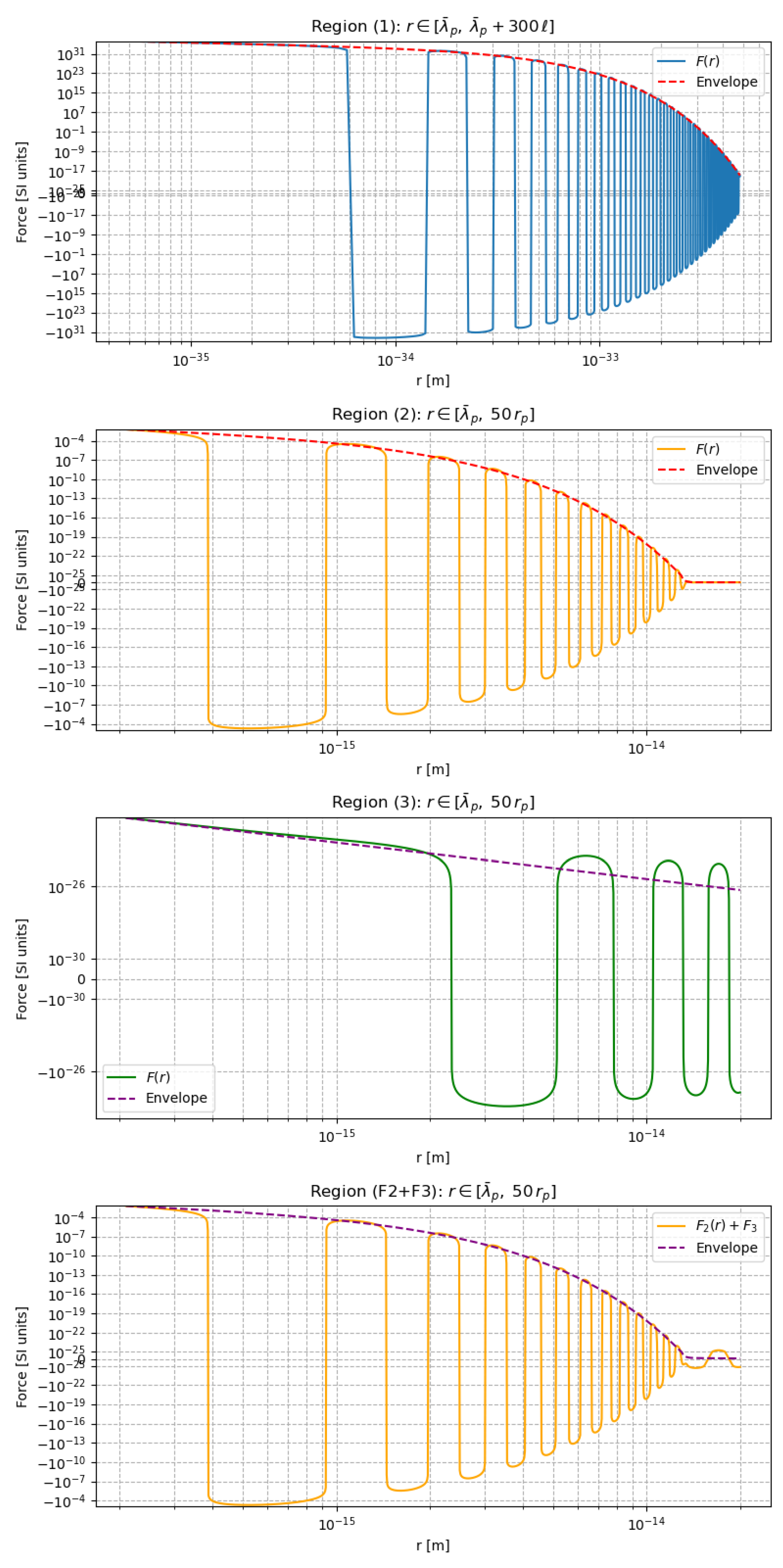
References
- Roberts, C.D. Origin of the proton mass. In Proceedings of the EPJ Web of conferences. EDP Sciences, 2023, Vol. 282, p. 01006. [CrossRef]
- Editorial. Proton Puzzles. Nature Review Physics 2021, 3. [CrossRef]
- Wilczek, F. Origins of mass. Open Physics 2012, 10. [CrossRef]
- Cho, A. Mass of the common quark finally nailed down. Science Magazine 2010, 201004. [CrossRef]
- Deur, A.; Brodsky, S.J.; de Teramond, G.F. The QCD running coupling. Progress in Particle and Nuclear Physics 2016, 90, 1–74. [CrossRef]
- Gell-Mann, M. A schematic model of baryons and mesons. Physics Letters B 1964, 8, 1–4. [CrossRef]
- Fritzsch, H.; Gell-Mann, M.; Leutwyler, H. Advantages of the color octet gluon picture. Physics Letters B 1973, 47, 365–368. [CrossRef]
- Gross, D.J.; Wilczek, F. Asymptotically free gauge theories. I. Physical Review D 1973, 8, 3633. [CrossRef]
- Shifman, M.A.; Vainshtein, A.I.; Zakharov, V.I. QCD and resonance physics. Theoretical foundations. Nuclear Physics B 1979, 147, 385–447. [CrossRef]
- Yang, Y.B.; Liang, J.; Bi, Y.J.; Chen, Y.; Draper, T.; Liu, K.F.; Liu, Z. Proton mass decomposition from the QCD energy momentum tensor. Physical review letters 2018, 121, 212001. [CrossRef]
- Durr, S.; Fodor, Z.; Frison, J.; Hoelbling, C.; Hoffmann, R.; Katz, S.D.; Krieg, S.; Kurth, T.; Lellouch, L.; Lippert, T.; et al. Ab initio determination of light hadron masses. Science 2008, 322, 1224–1227. [CrossRef]
- Ji, X. Breakup of hadron masses and the energy-momentum tensor of QCD. Physical Review D 1995, 52, 271. [CrossRef]
- Bali, G.S. QCD forces and heavy quark bound states. Physics Reports 2001, 343, 1–136. [CrossRef]
- Necco, S.; Sommer, R. Testing perturbation theory on the Nf= 0 static quark potential. Physics Letters B 2001, 523, 135–142. [CrossRef]
- Bazavov, A.; Toussaint, D.; Bernard, C.; Laiho, J.; DeTar, C.; Levkova, L.; Oktay, M.; Gottlieb, S.; Heller, U.; Hetrick, J.; et al. Nonperturbative QCD simulations with 2+ 1 flavors of improved staggered quarks. Reviews of modern physics 2010, 82, 1349–1417. [CrossRef]
- Metz, A.; Pasquini, B.; Rodini, S. Revisiting the proton mass decomposition. Physical Review D 2020, 102, 114042. [CrossRef]
- Burkert, V.D.; Elouadrhiri, L.; Girod, F.; Lorcé, C.; Schweitzer, P.; Shanahan, P. Colloquium: Gravitational form factors of the proton. Reviews of Modern Physics 2023, 95, 041002. [CrossRef]
- Dirac, P.A.M. Classical theory of radiating electrons. Proceedings of the Royal Society of London. Series A. Mathematical and Physical Sciences 1938, 167, 148–169. [CrossRef]
- Dyson, F.J. Divergence of perturbation theory in quantum electrodynamics. Physical Review 1952, 85, 631. [CrossRef]
- Bethe, H.A. The Electromagnetic Shift of Energy Levels. Phys. Rev. 1947, 72, 339–341. [CrossRef]
- Schwinger, J. On quantum-electrodynamics and the magnetic moment of the electron. Physical Review 1948, 73, 416. [CrossRef]
- Weinberg, S. The quantum theory of fields; Vol. 2, Cambridge university press, 1995.
- Einstein, A. The field equations of gravitation. Sitzungsber. Preuss. Akad. Wiss. Berlin (Math. Phys.) 1915, 1915, 844–847.
- Landau, L.D. The classical theory of fields; Vol. 2, Elsevier, 2013.
- Wilczek, F. Mass Without Mass I: Most of Matter. Physics Today 1999, 52, 11–13. [CrossRef]
- Einstein, A.; Rosen, N. The Particle Problem in the General Theory of Relativity. Phys. Rev. 1935, 48, 73–77. [CrossRef]
- Maldacena, J.; Susskind, L. Cool horizons for entangled black holes. Fortschritte der Physik 2013, 61, 781–811. [CrossRef]
- Donoghue, J.F.; Menezes, G. Inducing the Einstein action in QCD-like theories. Physical Review D 2018, 97, 056022. [CrossRef]
- Greene, B.R.; Morrison, D.R.; Polchinski, J. String theory. Proceedings of the National Academy of Sciences 1998, 95, 11039–11040.
- Maldacena, J. The large-N limit of superconformal field theories and supergravity. International journal of theoretical physics 1999, 38, 1113–1133. [CrossRef]
- Susskind, L. The anthropic landscape of string theory. arXiv preprint hep-th/0302219 2003.
- Rovelli, C.; Smolin, L. Loop space representation of quantum general relativity. Nuclear Physics B 1990, 331, 80–152. [CrossRef]
- Ashtekar, A.; Lewandowski, J. Background independent quantum gravity: a status report. Classical and Quantum Gravity 2004, 21, R53. [CrossRef]
- Amelino-Camelia, G. Quantum-gravity phenomenology: Status and prospects. Modern Physics Letters A 2002, 17, 899–922. [CrossRef]
- Loll, R. Quantum gravity from causal dynamical triangulations: a review. Classical and Quantum Gravity 2019, 37, 013002. [CrossRef]
- Planck, M. Über die Begründung des Gesetzes der schwarzen Strahlung. Ann. Phys. 1912, 342, 642–656. [CrossRef]
- Milonni, P.W. An Introduction to Quantum Optics and Quantum Fluctuations, 1 ed.; Oxford University PressOxford, 2019-01-31. [CrossRef]
- Milonni, P.W.; Shih, M.L. Zero-point energy in early quantum theory. American Journal of Physics 1991-08, 59, 684–698. [CrossRef]
- Kragh, H. Dirac: a scientific biography; Cambridge University Press, 1990.
- Lamb Jr, W.E.; Retherford, R.C. Fine structure of the hydrogen atom by a microwave method. Physical Review 1947, 72, 241. [CrossRef]
- Lamoreaux, S.K. Demonstration of the Casimir force in the 0.6 to 6 μ m range. Physical Review Letters 1997, 78, 5. [CrossRef]
- Bordag, M.; Mohideen, U.; Mostepanenko, V.M. New Developments in the Casimir Effect. Physics Reports 2001-10, 353, 1–205, [quant-ph/0106045]. [CrossRef]
- Anderson, C.D. The Apparent Existence of Easily Deflectable Positives. Science 1932-09-09, 76, 238–239. [CrossRef]
- Wheeler, J.A. On the nature of quantum geometrodynamics. Annals of Physics 1957-12, 2, 604–614. [CrossRef]
- Sakharov, A.D. Vacuum quantum fluctuations in curved space and the theory of gravitation. In Proceedings of the Doklady Akademii Nauk. Russian Academy of Sciences, 1967, Vol. 177, pp. 70–71.
- Adler, S.L. Einstein gravity as a symmetry-breaking effect in quantum field theory. Reviews of Modern Physics 1982, 54, 729. [CrossRef]
- Zel’dovich, Y.B. Electromagnetic and gravitational waves in a stationary magnetic field. Zh. Eksp. Teor. Fiz 1973, 65, 1311.
- Gertsenshtein, M. Wave resonance of light and gravitional waves. Sov Phys JETP 1962, 14, 84–85.
- Boccaletti, D.; De Sabbata, V.; Fortini, P.; Gualdi, C. Conversion of photons into gravitons and vice versa in a static electromagnetic field. Il Nuovo Cimento B (1965-1970) 1970, 70, 129–146. [CrossRef]
- Hawking, S.W. Gravitational Radiation from Colliding Black Holes. Phys. Rev. Lett. 1971-05-24, 26, 1344–1346. [CrossRef]
- Yukawa, H. On the interaction of elementary particles. I. Proceedings of the Physico-Mathematical Society of Japan. 3rd Series 1935, 17, 48–57. [CrossRef]
- Milonni, P.W. The quantum vacuum: an introduction to quantum electrodynamics; Academic press, 1993.
- Glauber, R.J. The quantum theory of optical coherence. Physical Review 1963, 130, 2529. [CrossRef]
- Bochove, E.J. Quantum theory of phase-conjugate mirrors. Journal of the Optical Society of America B 1992, 9, 266–280.
- Hawking, S.W. Particle creation by black holes. Communications in mathematical physics 1975, 43, 199–220.
- Hooft, G. The holographic principle. In Basics and Highlights in Fundamental Physics; World Scientific, 2001; pp. 72–100.
- Bigatti, D.; Susskind, L. TASI lectures on the holographic principle. In Strings, branes and gravity; World Scientific, 2001; pp. 883–933.
- Hawking, S.W. Virtual Black Holes. Phys. Rev. D 1996-03-15, 53, 3099–3107, [hep-th/9510029]. [CrossRef]
- Feynman, R.P. QED: The strange theory of light and matter; Vol. 90, Princeton University Press, 1985.
- Bekenstein, J.D. Universal upper bound on the entropy-to-energy ratio for bounded systems. Phys. Rev. D 1981-01-15, 23, 287–298. [CrossRef]
- Rafelski, J. Discovery of quark-gluon plasma: strangeness diaries. The European Physical Journal Special Topics 2020, 229, 1–140. [CrossRef]
- Karsch, F., Lattice QCD at high temperature and density. In Lectures on quark matter; Springer, 2002; pp. 209–249. [CrossRef]
- Sinha, K.P.; Sivaram, C.; Sudarshan, E.C.G. The superfluid vacuum state, time-varying cosmological constant, and nonsingular cosmological models. Found Phys 1976-12, 6, 717–726. [CrossRef]
- Weinberg, S. The quantum theory of fields; Cambridge University Press, 1995.
- Shanahan, P.; Detmold, W. Pressure distribution and shear forces inside the proton. Physical Review Letters 2019, 122, 072003. [CrossRef]
- Burkert, V.D.; Elouadrhiri, L.; Girod, F.X. The pressure distribution inside the proton. Nature 2018-05, 557, 396–399. [CrossRef]
- Haramein, N. Quantum Gravity and the Holographic Mass. Physical Science International Journal 2013, 3, 270–292.
- Lin, Y.H.; Hammer, H.W.; Meißner, U.G. New Insights into the Nucleon’s Electromagnetic Structure. Phys. Rev. Lett. 2022-02-03, 128, 052002. Publisher: American Physical Society, . [CrossRef]
- Haramein, N. Quantum Gravity and the Holographic Mass, Quantum. Physical Review & Research International 2013, pp. 2231–1815.
- Thorne, K.S.; Wheeler, J.A.; Misner, C.W. Gravitation; Freeman San Francisco, CA, 1971.
- Landau, L.D.; Lifshits, E.M.; Lifshits, E.M. Mechanics; Vol. 1, CUP Archive, 1960.
- Susskind, L. Cosmic Natural Selection, 2004-07-29, [hep-th/0407266].
- Yuan, G.W.; Lei, L.; Wang, Y.Z.; Wang, B.; Wang, Y.Y.; Chen, C.; Shen, Z.Q.; Cai, Y.F.; Fan, Y.Z. Rapidly growing primordial black holes as seeds of the massive high-redshift JWST Galaxies. arXiv 2023. [CrossRef]
- Harada, T.; Yoo, C.M.; Kohri, K. Threshold of primordial black hole formation. Physical Review D 2013, 88, 084051. [CrossRef]
- Dvali, G.; Gomez, C. Black holes as critical point of quantum phase transition. The European Physical Journal C 2014, 74, 1–12. [CrossRef]
- Davies, P.C.W. Thermodynamic phase transitions of Kerr-Newman black holes in de Sitter space. Class. Quantum Grav. 1989-12-01, 6, 1909–1914. [CrossRef]
- Hawking, S.W. Black hole explosions? Nature 1974-03-01, 248, 30–31. [CrossRef]
- Wheeler, J.A. Geons. Phys. Rev. 1955-01-15, 97, 511–536. [CrossRef]
- Brill, D.R.; Hartle, J.B. Method of the Self-Consistent Field in General Relativity and its Application to the Gravitational Geon. Phys. Rev. 1964-07-13, 135, B271–B278. [CrossRef]
- Maiani, L. The J/Ψ as a probe of Quark-Gluon Plasma. Lectures given at the International School of Subnuclear Physics, Trapani, Italy 2004.
- Langacker, P. Grand unified theories. In Proceedings of the International Symposium on Lepton and Photon Interactions at High Energies, Bonn. Citeseer, 1981.
- Burkert, V.; Elouadrhiri, L.; Girod, F. The pressure distribution inside the proton. Nature 2018, 557, 396–399. [CrossRef]
- Antoniadis, I.; Baessler, S.; Büchner, M.; Fedorov, V.; Hoedl, S.; Lambrecht, A.; Nesvizhevsky, V.; Pignol, G.; Protasov, K.; Reynaud, S.; et al. Short-range fundamental forces. Comptes Rendus Physique 2011, 12, 755–778. [CrossRef]
- Baker, A.; Haramein, N.; Alirol, O. The electron and the holographic mass solution. Physics Essays 2019, 32.
- Haramein, N.; Baker, A.V. Resolving the vacuum catastrophe: a generalized holographic approach. Journal of High Energy Physics, Gravitation and Cosmology 2019, 5, 412–424. [CrossRef]
- Özel, F.; Freire, P. Masses, radii, and the equation of state of neutron stars. Annual Review of Astronomy and Astrophysics 2016, 54, 401–440. [CrossRef]
- Fritzsch, H. Quarks: the stuff of matter; 1983.
- Suganuma, H.; Iritani, T.; Okiharu, F.; Takahashi, T.T.; Yamamoto, A. Lattice QCD study for confinement in hadrons. In Proceedings of the AIP Conference Proceedings. American Institute of Physics, 2011, Vol. 1388, pp. 195–201.
- Bali, G.S.; Schilling, K. Running coupling and the Λ parameter from SU (3) lattice simulations. Physical Review D 1993, 47, 661. [CrossRef]
- Baker, M.; Cea, P.; Chelnokov, V.; Cosmai, L.; Cuteri, F.; Papa, A. The confining color field in SU (3) gauge theory. The European Physical Journal C 2020, 80, 514. [CrossRef]
- Otsuka, T.; Abe, T.; Yoshida, T.; Tsunoda, Y.; Shimizu, N.; Itagaki, N.; Utsuno, Y.; Vary, J.; Maris, P.; Ueno, H. α-Clustering in atomic nuclei from first principles with statistical learning and the Hoyle state character. Nat Commun 2022-04-27, 13, 2234. [CrossRef]
- Ebran, J.P.; Khan, E.; Nikšić, T.; Vretenar, D. How atomic nuclei cluster. Nature 2012-07-19, 487, 341–344. [CrossRef]
- Carr, B.J.; Rees, M.J. The anthropic principle and the structure of the physical world. Nature 1979-04, 278, 605–612. [CrossRef]
- O’Raifeartaigh, C.; McCann, B.; Nahm, W.; Mitton, S. Einstein’s steady-state theory: an abandoned model of the cosmos. The European Physical Journal H 2014, 39, 353–367. [CrossRef]
- G, C.H.B. On the Attraction between Two Perfectly Conducting Plates. Proc. Kon. Ned. Akad. Wet. 1948, 51, 793.
- Garrett, J.L.; Somers, D.A.; Munday, J.N. Measurement of the Casimir Force between Two Spheres. Phys. Rev. Lett. 2018-01-23, 120, 040401. Publisher: American Physical Society, . [CrossRef]
- Lambrecht, A.; Reynaud, S. Casimir force between metallic mirrors. The European Physical Journal D 2000, 8, 309–318. [CrossRef]
- Munday, J.N.; Iannuzzi, D.; Barash, Y.; Capasso, F. Torque on birefringent plates induced by quantum fluctuations. Phys. Rev. A 2005-04-14, 71, 042102. [CrossRef]
- Chen, X.; Spence, J.C.H. On the measurement of the Casimir torque: On the measurement of the Casimir torque. Phys. Status Solidi B 2011-09, 248, 2064–2071. [CrossRef]
- Somers, D.A.T.; Garrett, J.L.; Palm, K.J.; Munday, J.N. Measurement of the Casimir torque. Nature 2018-12, 564, 386–389. [CrossRef]
- Guérout, R.; Genet, C.; Lambrecht, A.; Reynaud, S. Casimir torque between nanostructured plates. EPL 2015-08-01, 111, 44001. [CrossRef]
- Moore, G.T. Quantum Theory of the Electromagnetic Field in a Variable-Length One-Dimensional Cavity. Journal of Mathematical Physics 1970-09-01, 11, 2679–2691. [CrossRef]
- Wilson, C.M.; Johansson, G.; Pourkabirian, A.; Simoen, M.; Johansson, J.R.; Duty, T.; Nori, F.; Delsing, P. Observation of the dynamical Casimir effect in a superconducting circuit. Nature 2011-11, 479, 376–379. [CrossRef]
- Lähteenmäki, P.; Paraoanu, G.; Hassel, J.; Hakonen, P.J. Dynamical Casimir effect in a Josephson metamaterial. Proceedings of the National Academy of Sciences 2013, 110, 4234–4238. [CrossRef]
- Vezzoli, S.; Mussot, A.; Westerberg, N.; Kudlinski, A.; Dinparasti Saleh, H.; Prain, A.; Biancalana, F.; Lantz, E.; Faccio, D. Optical analogue of the dynamical Casimir effect in a dispersion-oscillating fibre. Communications Physics 2019, 2, 84. [CrossRef]
- Dodonov, V. Fifty Years of the Dynamical Casimir Effect. Physics 2020-02-14, 2, 67–104. [CrossRef]
- Altmannshofer, W.; Brod, J.; Schmaltz, M. Experimental constraints on the coupling of the Higgs boson to electrons. J. High Energ. Phys. 2015-05-25, 2015, 125. [CrossRef]
- Dirac, P.A.M. The quantum theory of the emission and absorption of radiation. Proc. R. Soc. Lond. A 1927-03, 114, 243–265. [CrossRef]
- Casimir, H.B.G.; Polder, D. The Influence of Retardation on the London-van der Waals Forces. Phys. Rev. 1948-02-15, 73, 360–372. [CrossRef]
- Sauter, F. Über das Verhalten eines Elektrons im homogenen elektrischen Feld nach der relativistischen Theorie Diracs. Z. Physik 1931-11, 69, 742–764. [CrossRef]
- Schwinger, J. On Gauge Invariance and Vacuum Polarization. Phys. Rev. 1951-06-01, 82, 664–679. [CrossRef]
- Berdyugin, A.I.; Xin, N.; Gao, H.; Slizovskiy, S.; Dong, Z.; Bhattacharjee, S.; Kumaravadivel, P.; Xu, S.; Ponomarenko, L.A.; Holwill, M.; et al. Out-of-equilibrium criticalities in graphene superlattices. Science 2022-01-28, 375, 430–433. Publisher: American Association for the Advancement of Science, . [CrossRef]
- Schmitt, A.; Vallet, P.; Mele, D.; Rosticher, M.; Taniguchi, T.; Watanabe, K.; Bocquillon, E.; Fève, G.; Berroir, J.M.; Voisin, C.; et al. Mesoscopic Klein-Schwinger effect in graphene. Nat. Phys. 2023-06, 19, 830–835. [CrossRef]
- et al., S.C. Measurement of e+e- Momentum and Angular Distributions from Linearly Polarized Photon Collisions. Phys. Rev. Lett. 2021-07-27, 127, 052302. Publisher: American Physical Society, . [CrossRef]
- Breit, G.; Wheeler, J.A. Collision of two light quanta. Physical Review 1934, 46, 1087 . [CrossRef]
- Xu, Z.; Gao, X.; Bang, J.; Jacob, Z.; Li, T. Non-reciprocal energy transfer through the Casimir effect. Nature nanotechnology 2022, 17, 148–152. [CrossRef]
- Kirchhoff, G. I. On the relation between the radiating and absorbing powers of different bodies for light and heat. The London, Edinburgh, and Dublin Philosophical Magazine and Journal of Science 1860, 20, 1–21. [CrossRef]
- Einstein, A. Indeed, it seems to me that the observations regarding” blackbody radiation,” photoluminescence, production of cathode rays by ultraviolet. Annalen der Physik 1905, 17, 132–148.
- Millikan, R.A. A direct photoelectric determination of Planck’s" h". Physical Review 1916, 7, 355. [CrossRef]
- Lehnert, B. Some Consequences of Zero Point Energy. Journal of Electromagnetic Analysis and Applications 2014, 06, 319. Number: 10 Publisher: Scientific Research Publishing, . [CrossRef]
- ZEL’DOVICH, I. Amplification of cylindrical electromagnetic waves reflected from a rotating body. Soviet Physics-JETP 1972, 35, 1085–1087.
- Unruh, W.G. Notes on black-hole evaporation. Phys. Rev. D 1976-08-15, 14, 870–892. [CrossRef]
- Dirac, P.A.M. The quantum theory of the electron. Proc. R. Soc. Lond. A 1928-02, 117, 610–624. [CrossRef]
- Mignani, R.P.; Testa, V.; Caniulef, D.G.; Taverna, R.; Turolla, R.; Zane, S.; Wu, K.; Curto, G.L. Evidence of vacuum birefringence from the polarisation of the optical emission from an Isolated Neutron Star, 2018-02-14, [1710.08709 [astro-ph]].
- Pike, O.; Hill, E.; Rose, S.; Mackenroth, F. Observing the two-photon Breit-Wheeler process for the first time. In Proceedings of the APS Division of Plasma Physics Meeting Abstracts, 2014, Vol. 2014, pp. UO7–007.
- Anderson, P.W. Plasmons, gauge invariance, and mass. Physical Review 1963, 130, 439. [CrossRef]
- Adler, R.J.; Casey, B.; Jacob, O.C. Vacuum catastrophe: An elementary exposition of the cosmological constant problem. American Journal of Physics 1995-07, 63, 620–626. [CrossRef]
| 1 | p.5-7 |
| 2 | p.36-41 |
| 3 | p.184 |
| 4 | p.128 |
| 5 | p.427-428 |
Figure 4.
(a) Schematic representation of the dual screening process that generates rest mass from quantum vacuum fluctuations. This process occurs at two distinct screening surfaces: (1) the Compton wavelength, which produces the proton core energy density, and (2) the proton charge radius, which results in the rest mass energy density. This hierarchical screening mechanism corresponds to phase transitions in the Planck Plasma, progressing from the initial Bose phase to the high-density (HD) and low-density (LD) Bose-Fermi phases. (b) Semi-permeable boundaries at the two screening surfaces ( and ) characterize phase transitions through elementary voxel aggregation into kernel-64 structures. This process screens vacuum fluctuations, transforming the vacuum energy density () first into the proton black hole density () and subsequently into the rest mass energy density ().
Figure 5.
Evolution of three fundamental forces—color confinement, residual strong, and gravitational—arising from gravitational waves induced by Planck-scale quantum vacuum fluctuations. This plot illustrates the dual screening mechanism originating from the Planck force ground state . The inset magnifies the first screening transition (blue line), plotted in Planck length units from the Compton wavelength horizon . Key features include the color confinement force reaching N at the proton radius and the residual strong force measuring N at the characteristic inter-nucleon separation of during the second screening phase transition (orange line). For comparison, the electrostatic Coulomb force (green line) and Newtonian gravitational force (purple line) are also displayed.
Table 3.
Mass and Radius Scaling Relations
| Proton | Universe | |
|---|---|---|
| Mass | ||
| Radius |
Disclaimer/Publisher’s Note: The statements, opinions and data contained in all publications are solely those of the individual author(s) and contributor(s) and not of MDPI and/or the editor(s). MDPI and/or the editor(s) disclaim responsibility for any injury to people or property resulting from any ideas, methods, instructions or products referred to in the content. |
© 2025 by the authors. Licensee MDPI, Basel, Switzerland. This article is an open access article distributed under the terms and conditions of the Creative Commons Attribution (CC BY) license (http://creativecommons.org/licenses/by/4.0/).
Copyright: This open access article is published under a Creative Commons CC BY 4.0 license, which permit the free download, distribution, and reuse, provided that the author and preprint are cited in any reuse.


