
Submitted:
21 September 2025
Posted:
23 September 2025
You are already at the latest version
Abstract
This paper is concerned with the vibrations of a mass connected to a wall or ground via a linear spring and a viscous damper arranged in series. Discrete models used to investigate the vibrations of machinery and structures often consist of a mass supported by a spring and damper in parallel or a series combination of such a system. However, models in which the spring and damper are connected in series are rarely encountered. To the authors' knowledge, there are no publications solely focused on the vibrations of a mass supported by a spring and a damper in series. In this paper, we demonstrate that the vibrational behaviour of such a system is entirely different from a system that comprises a mass with a parallel spring and damper combination. In contrast to the parallel combination, vibrations occur in this system when the damping ratio is greater than one. Another distinct result is that when the ratio of excitation frequency to the natural frequency of the system is set to zero, the frequency response function of the system with a serial combination goes to infinity. Thus, it does not correspond to the static loading case, unlike the system with a parallel combination. Furthermore, the transmissibility curves in such a system do not intersect at a certain value of the ratio of frequencies, whereas in the system with a parallel combination, these curves intersect when the ratios of frequencies are equal to 2. The system under consideration can suppress natural vibrations even for very small damping ratios, implying that this system can be used to control horizontal vibrations of a structure.
Keywords:
mechanical vibrations
; one-degree-of-freedom system
; serial spring-damper configuration
; mass-spring-damper model
; natural frequency
; critical damping
; free vibrations
; forced vibrations
. The system under consideration can suppress natural vibrations even for very small damping ratios, implying that this system can be used to control horizontal vibrations of a structure.
1. Introduction
An elementary mechanical vibration course starts with the introduction of system parameters which are required to be determined when one desires to study a mechanical system in vibration. These are inertia, restoring force and dissipative elements, in other words, mass (or mass moment of inertia), springs, (or gravity) and dampers (or dashpot). These parameters (or features) can be assumed to be distributed or discretized throughout the structure depending on the level of complexity of the model to be established. For continuum models, parameters are distributed over the whole system while, for simple and discrete models, parameters are localized at certain regions of model. The fundamental concepts and definitions in the theory of vibration are usually given using a one degree of freedom discrete model which consists of a mass supported by a linear spring and linear viscous damper in parallel. This model is also used to study the vibratory behaviour of many applications in the practice [1,2,3,4]. For example, vibration isolation of a machine, suspension system of a vehicle, design of machine foundation can be studied by means of this model. Although the combination of spring and damper in series in this model is possible, one does not explain why the parallel combination is chosen or preferred. Spring and damper elements are not only used in vibration theory. Also in materials science, there exist some models in which springs and dampers are used to represent the viscoelastic behaviour of a material, such as the Maxwell [5], Kelvin-Voigt [6], and Zener [7] models. For example, the Maxwell model defines the stress-strain relationship of a material using a linear spring and a Newtonian damper connected in series, while the Kelvin-Voigt model employs a linear spring and a dashpot arranged in parallel. The Zener model, on the other hand, comprises a parallel combination of a linear spring and a group of another spring and dashpot in series. In these material models, spring and damper forces correspond to stresses; therefore, they are functions of strain and strain rates, respectively [6,7]. These models are also employed to analyse the vibrational characteristics of mechanical systems [8,9,10].
Kumbhar et al. [11] present a detailed study of a novel semi-active air spring–air damper system designed for efficient vibration control in single-degree-of-freedom (SDOF) systems subjected to base excitation. They develop a Maxwell-type mathematical model to optimize parameters such as spring rate and damping ratio.
Bougteb and Ray [12] examine the effectiveness of series and parallel configurations of hysteretic systems and viscous dampers in seismic applications. Through response spectrum analyses of single-degree-of-freedom systems, they explore how these configurations impact base shear and ductility demand. It is shown that it provides insights into optimizing damping systems for seismic protection, with practical implementation suggestions for structural design.
According to the authors’ investigation using search engines and pertinent journal databases, however, no research has been found that solely focuses on studying the vibration characteristics of a mass connected to wall with a linear spring and a viscous damper in series. Motivated by this fact, this paper addresses the vibration characteristics of such a system. This study also enables us to understand why the parallel combination of spring and damper is preferred in technical applications.
The paper is organized as follows: The first section is devoted to deriving equations for two variants of the system, which comprises a mass connected to the wall or ground via a spring and damper in series. In addition, the free vibrations of these two variants are addressed. In the second section, forced vibrations of these systems are studied. The external excitation is presented in two different forms: a harmonic force acting on the mass and a harmonic displacement applied to the wall/ground. For both types of excitation, frequency response functions are obtained and discussed. Finally, transmissibility functions are derived, and some numerical examples are provided to enhance the understanding of the subject.
2. System Equations and Free Vibrations
As mentioned earlier, this paper focuses on the vibrations of a one-degree-of-freedom mechanical system in which a mass is connected to the wall or ground via a linear spring and damper in series. In such a system, the spring and damper between the wall or ground and the mass can be arranged in two different ways. For each configuration, we must determine the natural frequency and critical damping of the system. In this study, for simplicity, we assume that the mass moves horizontally back and forth without any friction between the mass and the surface, as depicted in Figure 1. Depending on the arrangement of the spring and damper between the wall and the mass, we can distinguish two different configurations, as illustrated in Figure 1a and 1b. We refer to them as the c-k-m variant and the k-c-m variant, respectively.
In both configurations, the displacements of the connection point of the spring and damper, as well as the mass, are denoted by and , respectively.
2.1. System Equations
First, we need to clearly define the reference points from which we measure the displacements and . In the initial positions of both systems, we assume that the spring is undeflected, and the rod of the damper is at the midpoint of its leftmost and rightmost positions. From Figure 1a, the equations of motion for the c-k-m variant are as follows:
(a)
(1)
(b)
In fact, Eq (1a) represents the equation of motion for the mass. The second equation, Eq (1b), can be interpreted as either a constraint equation or a matching condition. In this context, since we are dealing with two differential equations, the sum of whose orders is three, as some authors do, we can refer to this system as a one-and-a-half degree-of-freedom (d.o.f.) system. The equations of motion for the second variant, shown in Figure 1b, are derived as follows:
(a)
(2)
(b)
It is possible to solve these equations analytically by eliminating one of two variables and . For the first variant, if Eq (1b) is solved for , one finds:
By differentiating both sides of Eq (3) with respect to time, we get the following:
Substituting Eqs (3) and (4) into Eq (1a) and dividing all terms by the coefficient of the highest derivative yields a third-order differential equation in as follows:
where and are defined as
As is known from the theory of linear differential equations, we can propose a candidate solution to Eq (5) in the form of . If we substitute this into the equation, the characteristic equation is obtained:
According to Eq (8), the roots of Eq (8) are as follows:
(a)
(9)
(b)
(c)
If the expression under the square root sign is negative, vibrations can occur in the system. Therefore, the critical damping can be obtained by equating this expression to zero. The critical value of is then found as
If we recall Eq (6), the critical damping is obtained as follows:
We know that critical damping for a system with a spring and damper connected in parallel is . In order for the system to vibrate, the expression must be negative. This leads us to an interesting result: if , vibration will occur in the system, in complete contrast to the behaviour of a system with a parallel spring-damper combination. Now, we can define the damping ratio, as is customary in vibration theory.
Hence, the condition for the system vibration, can be replaced with the condition . Here, we call the natural frequency of system.
A similar procedure can be followed to solve Eqs (2). First, we solve Eq (2b) for :
Then, Eq (13) is differentiated w.r.t. time once more:
Eqs (13) and (14) are substituted in Eq (2a). After some rearrangement, one obtains the following differential equation in of second order:
the characteristic equation of which is the same as the expression in the parenthesis in Eq (8). Consequently, the critical damping is again given with Eq (11). Also, the condition that the system vibrates is or .
The equations given by both Eq (1) and Eq (2) are two differential equations, the orders of which are two and one, respectively. To solve them numerically, three initial conditions must be provided: , , . (Note that the ‘dot’ symbol indicates a time derivative). Using any differential equation solver, such as the fourth-order Runge-Kutta algorithm, these equations can be solved. In this case, the set of equations given by Eq (1) or Eq (2) must be reduced to a set of three first-order equations. These sets are obtained as follows:
For the c-k-m variant:
Where , and are defined as
For the k-c-m variant:
3. Forced Vibrations
In this section, two different cases will be investigated: System response to a harmonic force acting on the mass (force excitation), and system response to a harmonic displacement applied at the wall/ground (displacement excitation). Both force and displacement excitations are defined in the form of and , respectively. The displacement of the connection point of spring and damper, and the mass are denoted by and respectively, where and are complex amplitudes. The modula of and give the real amplitudes and .
3.1. Force Excitation
For the c-k-m variant, the equations of motion take the following form,
If the expressions mentioned above for and are used in Eqs (19), and the multiplier is eliminated from each term in the equations, the following equations are obtained for and :
If Eqs (20) are solved for and using a suitable method such as Cramer’s rule, the complex amplitudes and are found as follows:
where
and
Note that is the excitation frequency.
Regarding the k-c-m variant, the equations of motion are as follows:
Following the similar procedure described above, Eqs (25) are solved for and . For this case, and are given below:
(21-repeated)
For both variants, the complex amplitudes are the same. For a system in which spring and damper are attached to ground is parallel, the complex amplitude has the following form:
where . When is set to zero in Eq (27), is equal to . It means that, the response of the system with a parallel spring-damper combination to a static load is easily found by setting in Eq (27). However, this is not the case in the system in which spring and damper are connected to each other in series because the modulus of goes to infinity if is set to zero in Eq (21). From this result, it is concluded that the dimensions of the damper must be considered if one desires to find the static deflection of the system under a static load . Also, the stroke of the rod of the damper becomes important when we want to find the transient behaviour of the system, the stroke of the rod is again required. Otherwise, numerical solution of equation of motion may yield meaningless results.
3.2. Displacement Excitation
For the c-k-m variant, equations of motion are as follows:
If one substitutes and , and consider , the following equations are obtained after eliminating the term :
Solving Eqs (29) for and successively yields:
Also, for the k-c-m variant, equations of motion are obtained as below:
After necessary substitutions in Eqs (32), the following equations in and are found:
Then, and are obtained as follows:
(30-repeated)
For the displacement excitation, complex amplitudes are the same, as well.
There is an interesting point to note here. When is set to zero in Eqs (30) and (34), these expressions result in an indeterminate form, 0/0. However, upon applying L’Hopital’s rule to these expressions, we observe that . Another important point to emphasize is that for displacement excitations, complex amplitudes remain the same in both variants. It is worth recalling that the expressions , , and represent complex frequency response functions.
4. Transmissibility
Transmissibility is a measure of vibration isolation in machine foundations. It is defined as the ratio of the maximum value of the resulting event to the maximum value of the causing event, i.e., the ratio of amplitudes. In this section, we want to find the transmitted force through the support which consists of the combination of spring and damper in series when a harmonic force acts on the mass or the amplitude of vibration of the mass caused by the harmonic motion of the wall/ground.
4.1. Force Transmissibility
For the c-k-m variant, by definition, we can write
where , i.e., the modulus of the complex amplitude related to the c-k-m variant.
We can also write the following expression for the k-c-m variant:
Here, is the real amplitude for the k-c-m variant.
We observe that the force transmissibility for both variants are the same.
4.2. Displacement Transmissibility
The displacement transmissibility is defined as . Since the complex amplitudes ’s, hence the real amplitudes. ’s for both variants are the same, one has only one expression for the displacement transmissibility:
Eq (37) is equivalent to Eq (36), hence Eq (35). Consequently, we observe that the system considered has a unique transmissibility function regardless of the sequence of spring and damper, and the type of excitations.
5. Numerical Examples
In this section, we will provide and discuss numerical examples for each of the concepts discussed so far, including frequency response functions and transmissibility functions for both variants of the spring and damper combinations in series. Additionally, we will explore free vibrations of two variants for certain initial conditions.
5.1. Examples for Free Vibrations
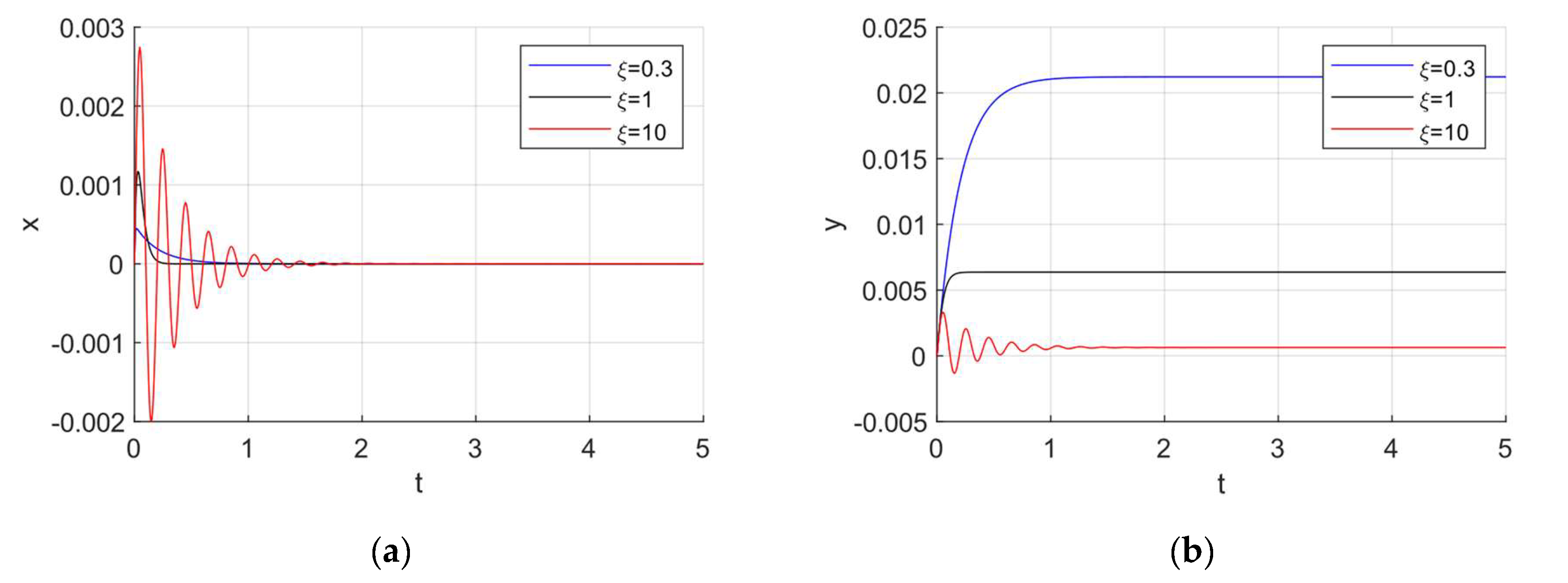
One example for each variant of the serial combination of spring and damper are presented. The initial conditions are selected as , and in these examples. For each variant, free vibration curves are plotted for four values: , ,, (). The variations of and over time are illustrated in Figure 2a and 2b for the c-k-m variant. As previously emphasized, vibrations occur only when , which is a noteworthy observation. This phenomenon can be explained by the fact that when , the damper gets stiffer, and in the limiting case it behaves like wall or ground. Thus, the mass vibrates as if it is directly connected to the wall by a spring. The system response curves for the k-c-m variant are shown in Figure 3a and 3b. Once again, we observe a dynamic behaviour similar to the former when . The mass performs a free, damped vibration. This event can be explained as before: Values of greater than correspond to a stiffer damper, causing the mass and the damper to move as if they were one body.
5.2. Examples for Forced Vibrations
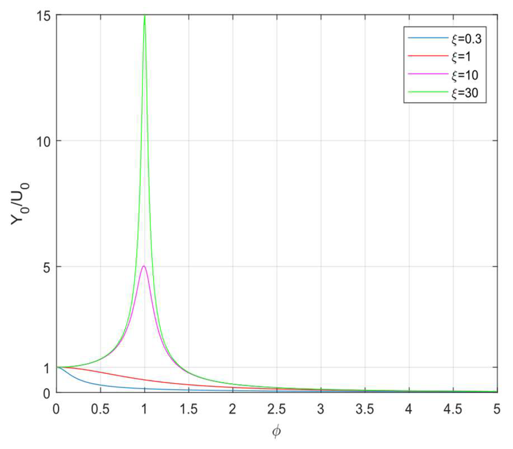
In these examples, zero initial conditions are assumed, i.e., . takes the same values as in the case of free vibrations. The frequency response functions for both force and displacement excitations are plotted. The sequence of spring and damper in the combination does not affect the frequency response functions for each type of excitation. Consequently, we have two separate frequency response functions, one for force excitation and the other for displacement excitation as shown in Figure 5 and 6, respectively.
Figure 4.
This is a figure. Schemes follow the same formatting.
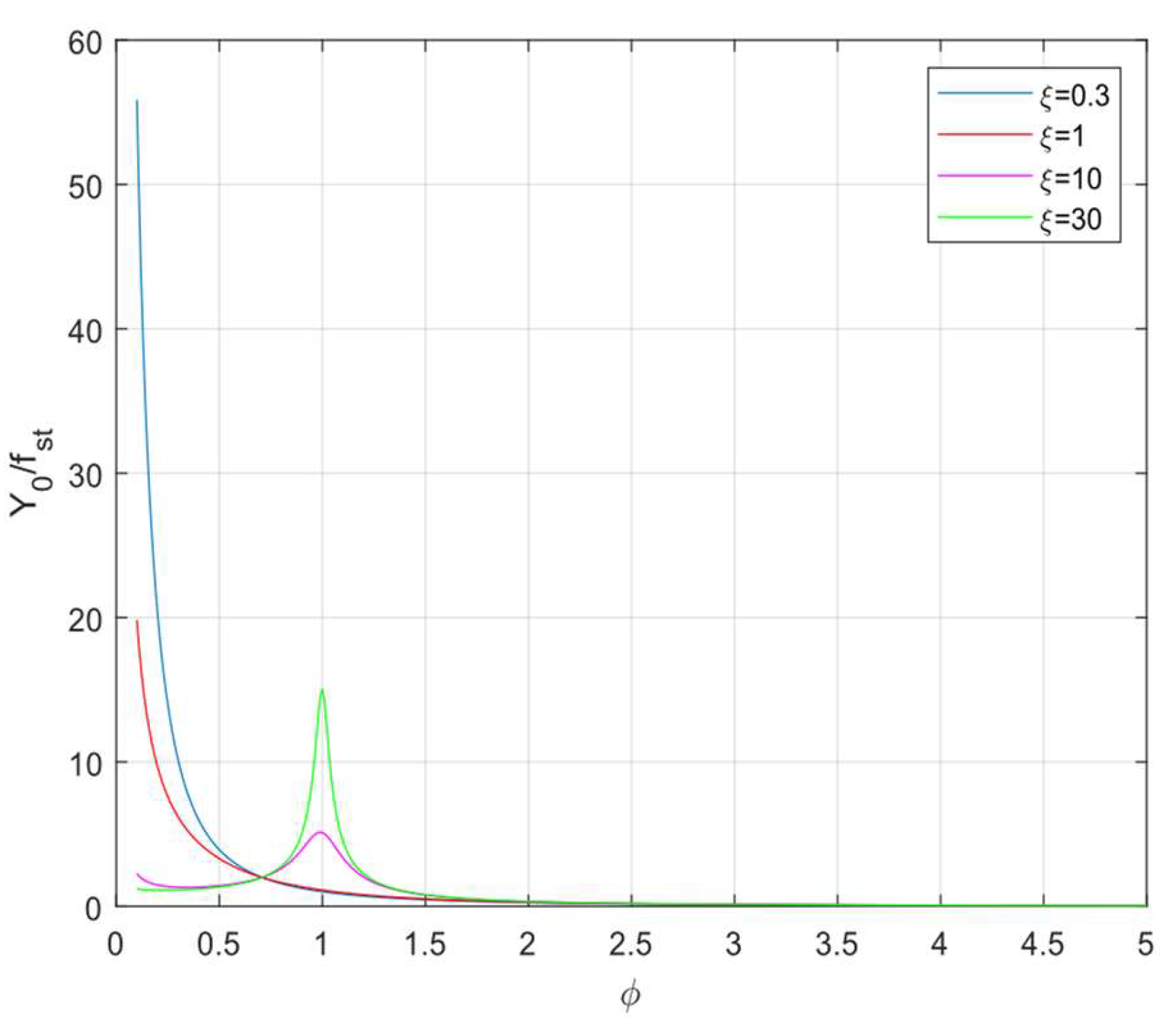
Figure 5.
This is a figure. Schemes follow the same formatting.
5.3. Examples for Transmissibility
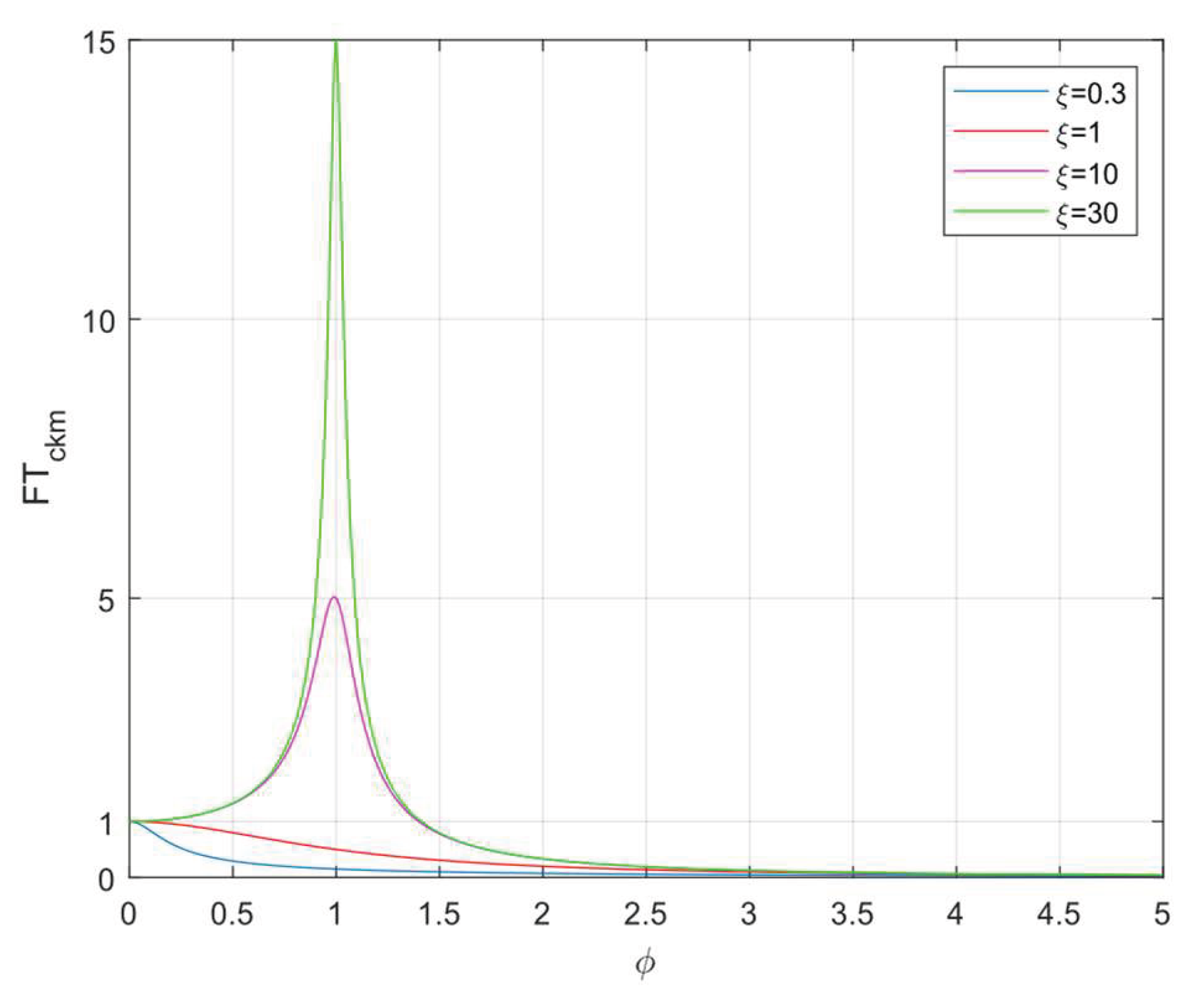
The only transmissibility chart valid for both variant is plotted in Figure 7. In this graphics, one does not encounter an intersection point of the transmissibility curves for different -values unlike the system with the parallel spring-damper combination (In that case, for , the damping becomes immaterial).
Figure 6.
This is a figure. Schemes follow the same formatting.
6. Conclusion
As revealed by the theory and numerical examples presented in the preceding sections, the serial combination of spring and damper in a mass-spring-damper system leads to a dynamical behaviour completely different from that of a one dof system in which spring and damper are placed in parallel. The significant conclusions drawn from this study are listed below:
-In the system in which a mass is attached or supported to wall or ground with a linear spring and linear viscous damper in series, the critical damping coefficient is , which is one forth the critical damping of the system with the parallel combination of spring and damper where .
-In the system studied here, free vibration occur when in contrast to the system with parallel spring and damper where no free vibrations exist for . This phenomenon can be explained by the fact that large damping ratios correspond to stiffer damper, which means that the damper behaves as if it were just one piece with the wall or the mass.
-The frequency response curves for force excitation do not take the value 1 for unlike the system with parallel spring and damper. Therefore, for the system considered here, it is not possible to transition from the dynamic loading case to the static one. To overcome this difficulty the dimensions of the damper must be considered. This helps us understand why this serial combination is not used in vehicle suspensions; in the parallel combination, the static load can be carried by the spring, so the damper does not undergo any load.
-The frequency response curves for displacement excitation have the value 1 for . However, if we directly substitute in Eq (39), it gives an indeterminacy of 0/0. Using L’Hopital’s rule, it can be shown that the frequency response function takes the value at .
-As in the case of one-degree-of-freedom system with parallel spring and damper, there exist a unique transmissibility function valid for both force and displacement excitations. However, the transmissibility curve for different values do not intersect each other at any value of why, they intersect at for a parallel spring and damper combination. That means the damping ratio becomes insignificant.
-In the system studied here, quite a small amount of damping is sufficient to suppress natural vibrations and reduce forced vibration amplitudes, unlike the one-degree-of-freedom system with a parallel spring and damper combination.
To simplify the mathematical complexity of the model, the system is assumed to move horizontally. However, this type of application can be used to control the undesired horizontal vibrations of a building or structure because it does not require large damping. The authors continue such a work.
Author Contributions
Conceptualization, E.D. and O.K.; methodology, E.D. and O.K.; software, E.D. and O.K.; validation, E.D.; formal analysis, E.D. and O.K.; investigation, E.D.; resources, E.D.; data curation, E.D.; writing—original draft preparation, E.D. and O.K.; writing—review and editing, E.D. and O.K.; visualization, E.D.; supervision, O.K. All authors have read and agreed to the published version of the manuscript.
Funding
This research received no external funding.
Institutional Review Board Statement
Not applicable.
Informed Consent Statement
Informed consent was obtained from all subjects involved in the study.
Data Availability Statement
No new data were created or analyzed in this study. Data sharing is not applicable to this article.
Conflicts of Interest
The authors declare no conflicts of interest.
References
- Meirovitch, Leonard. Fundamentals of vibrations. Waveland Press, 2010.
- Thomson, William Tyrrell. Theory of Vibrations with Applications. India: Pearson Education, 2008.
- Rao, Singiresu. Mechanical Vibrations. United Kingdom: Pearson Education, Incorporated, 2017.
- Balachandran, Balakumar, and Magrab, Edward B. Vibrations. United Kingdom: Cambridge University Press, 2018.
- Maxwell, J. C. (1867). “On the dynamical theory of gases.” Philosophical transactions of the Royal Society of London, (157), 49-88.
- Banks, Harvey Thomas, Shuhua Hu, and Zackary R. Kenz. “A brief review of elasticity and viscoelasticity for solids.” Advances in Applied Mathematics and Mechanics 3, no. 1 (2011): 1-51.
- Zener, Clarence M., and Sidney Siegel. “Elasticity and Anelasticity of Metals.” The Journal of Physical Chemistry 53, no. 9 (1949): 1468-1468.
- Biancolini, Marco Evangelos, Carlo Brutti, Dario Del Pin, and Luigi Reccia. “Three-dimensional dynamic model for a quick simulation of vehicle collisions.” No. 2001-01-3212. SAE Technical Paper, 2001.
- Oryński, Franciszek, and Witold Pawłowski. “The influence of grinding process on forced vibration damping in the headstock of a grinding wheel of a cylindrical grinder.” International Journal of Machine Tools and Manufacture 39, no. 2 (1999): 229-235.
- Brennan, M. J., A. Carrella, T. P. Waters, and Vicente Lopes Jr. “On the dynamic behavior of a mass supported by a parallel combination of a spring and an elastically connected damper.” Journal of Sound and Vibration 309, no. 8: 3-5 (2008), 2008. [Google Scholar]
- Kumbhar, M. B. , Salunkhe, V. G., Borgaonkar, A. V., and Jagadeesha, T. (2021). “Mathematical modeling and experimental evaluation of an air spring–air damper dynamic vibration absorber.” Journal of Vibration Engineering & Technologies, 9(3), 781–789. [CrossRef]
- Bougteb, Y. , and Ray, T. (2017). “Choice between series and parallel connections of hysteretic system and viscous damper for seismic protection of structures.” Earthquake Engineering and Structural Dynamics. [CrossRef]
Figure 1.
This is a figure. Schemes follow the same formatting.
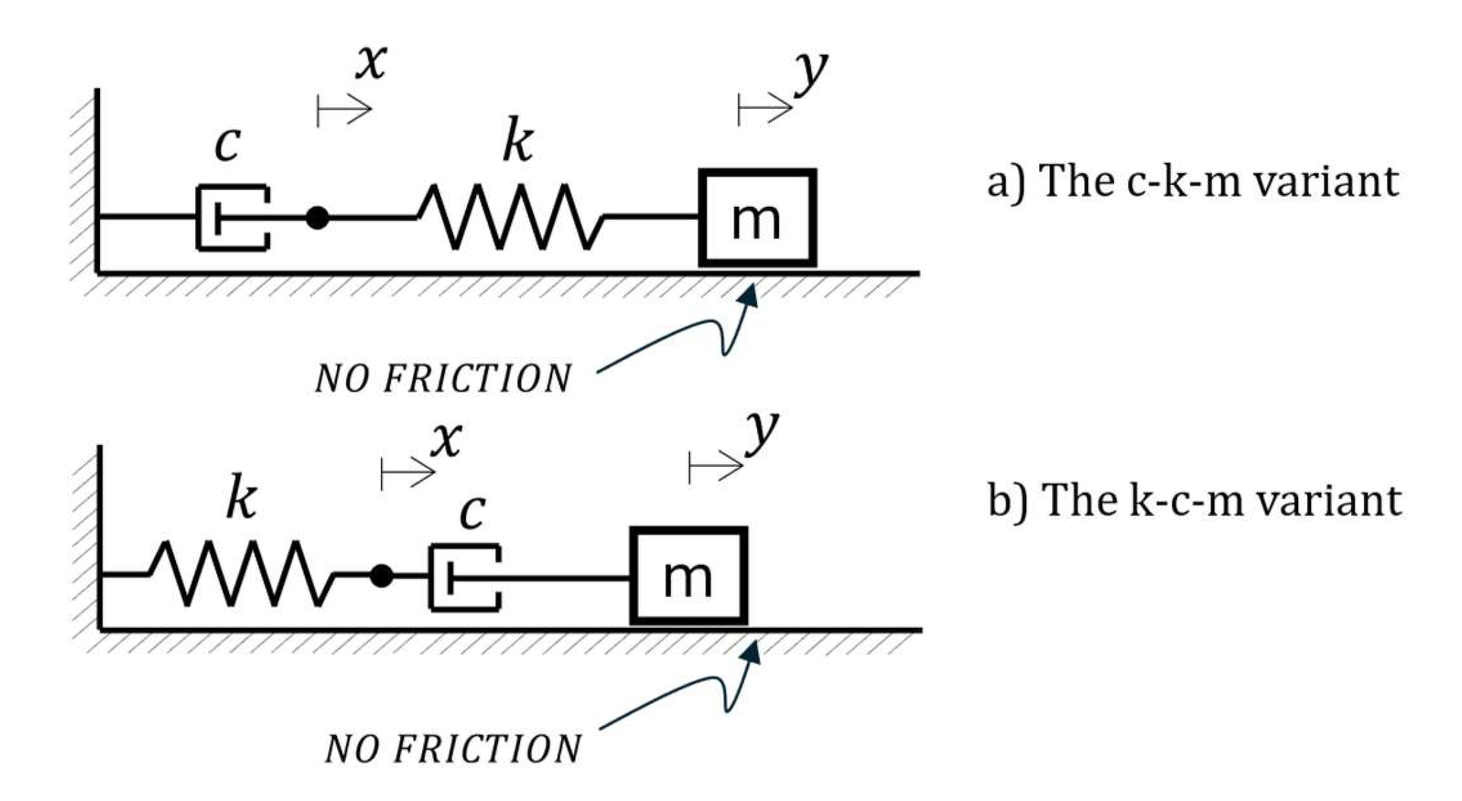
Figure 2.
This is a figure. Schemes follow another format. If there are multiple panels, they should be listed as: (a) Description of what is contained in the first panel; (b) Description of what is contained in the second panel. Figures should be placed in the main text near to the first time they are cited.
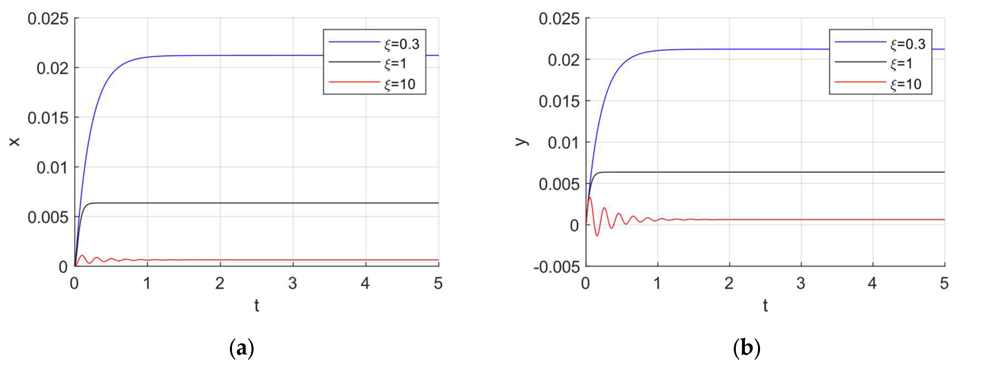
Figure 3.
This is a figure. Schemes follow another format. If there are multiple panels, they should be listed as: (a) Description of what is contained in the first panel; (b) Description of what is contained in the second panel. Figures should be placed in the main text near to the first time they are cited.
Disclaimer/Publisher’s Note: The statements, opinions and data contained in all publications are solely those of the individual author(s) and contributor(s) and not of MDPI and/or the editor(s). MDPI and/or the editor(s) disclaim responsibility for any injury to people or property resulting from any ideas, methods, instructions or products referred to in the content. |
© 2025 by the authors. Licensee MDPI, Basel, Switzerland. This article is an open access article distributed under the terms and conditions of the Creative Commons Attribution (CC BY) license (http://creativecommons.org/licenses/by/4.0/).
Copyright: This open access article is published under a Creative Commons CC BY 4.0 license, which permit the free download, distribution, and reuse, provided that the author and preprint are cited in any reuse.


