Optimal Design Methodology of Maxwell Coulomb Friction Damper

1. Introduction

The response of a SDOF system subjected to harmonic excitation to which tuned mass damper with traditional linear stiffness and dry friction damping arrangement is considered by Ricciardelli and Vickery (1999). Its optimal solution brings to a standard response curve almost flat in a broad range of frequencies. To tune up its resonant frequency at the optimal value, an additional spring is configured in our development. As the damping force is direction sensitive, relative motion directions are considered in its transmissibility formulation. Tunable friction damper was established by Lee et al. (2005) using viscous and Coulomb elements in parallel arrangement. It was designed to work as friction damper while the mass slips and as vibration absorber while the mass sticks. However, it involved more complicated viscous component.

In the work of Brizardet. al. (2013), a friction damper was designed and a prototype was built to reduce engine vibrations on a space launcher. The friction damper was modelled by a spring in series with a friction element. The damper prototype proved to efficiently damp the rocket engine vibrations.And the design method used for dimensioning the friction damper gave approximation for the optimal sliding force of the damper. The adaptive friction damper prototype enables to adjust the sliding force by controlling the normal force. For our optimal design process, the damper spring and friction element are arranged in Maxwell configuration similarly. However, not just the energies related to the damper are considered. The performance of its transmissibility is one of the utmost factors used in our design. Its derivative at the specific level is employed to optimize its stiffness ratio as another factor. Simultaneously, its damping ratio is optimized using force ratio between the Coulomb force and the applied force.

Research efforts were put to solve the Maxwell type damper arrangement in the DVA research areas. The response of SDOF spring mass system connected to vibration absorber with flexible friction damper and subjected to sinusoidal excitation was considered by Sinha and Trikutam (2018). Its flexible friction damper was of Maxwell configuration in 2DOF system. Meanwhile its motion equations were derived using L-P method commonly used in nonlinear vibration. Then they were solved numerically by an ordinary differential equation (ODE) method. The friction damper was used by Wang and Chen (1993) to reduce the maximum vibration of engine blade. Although the harmonic balance method (HBM) was well-known method for studying nonlinear vibration problems, generally only a one-term approximation was proposed to study the nonlinear vibration of a frictionally damped blade. In their work, a HMB procedure with a multiterm approximation was proposed. The results show that the steady-state response and other related behaviour of frictionally damped blade was predicted accurately and quickly by an HBM with a multiterm approximation. In this simulation, similar turbine blade is implemented to demonstrate the correctness of hysteresis loop generated by the central-difference solution. Various unconstrained central-difference search methods are developed to optimize turbine blade friction and stiffness.

A numerical method was developed by Hatada et. al. (2000) for the dynamic analysis of a tall building structure with viscous dampers in Maxwell configuration. Viscous dampers were installed between the top of an inverted V-shaped brace and the upper beam on each storey to reduce vibrations during strong disturbances like earthquakes. Third-order differential equation was established. The computational method was formulated by incorporating a finite element of the Maxwell model into the second-order ODE of motion in the discrete-time system. Bhaskararao and Jangid (2007) investigated dynamic behaviour of two identical adjacent structures connected with viscous dampers under base acceleration. Peak displacements and minimum inter-storey damping were obtained. Closed-form expressions for optimum damper damping of undamped structures were applied to damped structure. The governing differential equations of motion of the coupled system were derived and solved for relative displacement and absolute acceleration responses by Patel and Jangid (2014). Parametric study was conducted to study the influence of important system parameters (such as excitation frequency, mass ratio, and stiffness ratio) on the response behaviour of damper connected structures. Chen and Wu (2022) investigated the seismic performance of two adjacent tower and podium connected by viscous dampers. Three types of damper placement are discussed, including installing dampers within a single building, connecting two buildings at the same floor level, and connecting two buildings at the inter-story level. In this effort, Maxwell Coulomb damper is applied to suppress the maximum displacement of adjacent tower and podium subjected to ground motions. Its performance is compared with viscous damper using equivalent damping ratios.

In this SDOF design, we discover that commonly used viscous damper is less effective for lower range damping ratio application. From the shape of contour graph, it appeared to straight lines. On the other side, Maxwell Coulomb damper gives concave downward contour as damping ratio decreases. As compared with viscous damper, its performance is better at lower range. Thus this damper can be a better alternative than viscous damper because of its low cost and ease of maintenance. However, friction damper was not as commonly used as viscous damper because its design involved nonlinear dynamics analysis. Also the pure Coulomb friction damper had the problem of zero or little damping effect to the vibration of spring-mass dynamic system at resonance where singularity occurring. With the combination of Maxwell spring, these gaps can be linked up by relatively convenient conversion using viscous equivalent damping coefficient, and less drastic and more stable motion under additional stiffness.

A mesh-free least-squares-based finite difference method was applied by Wu et al. (2008) for solving large-amplitude free vibration problem of arbitrarily shaped thin plates. Spatial derivatives of a function at a point are expressed as weighted sums of the function values of a group of supporting points. String/slider non-linear coupling system with time-dependent boundary condition was considered by Fong and Chang (2001). The finite difference method with variable grid was employed to show the numerical results of the coupling effect between the string and slider.Three-dimensional dynamics of long pipes towed underwater were analysed by Kheiri et al. (2013). In their finite difference scheme, partial differential equations of motion and boundary conditions were converted into a set of first-order ODEs. In our analysis, ODEs from four case models were solved separately using central-difference method. Then they were sequentially connected by initial displacements and velocities.

2. System Modelling and Central-Difference Solver of Coulomb Damper

2.1. System Modelling of Coulomb Friction and Viscous Dampers

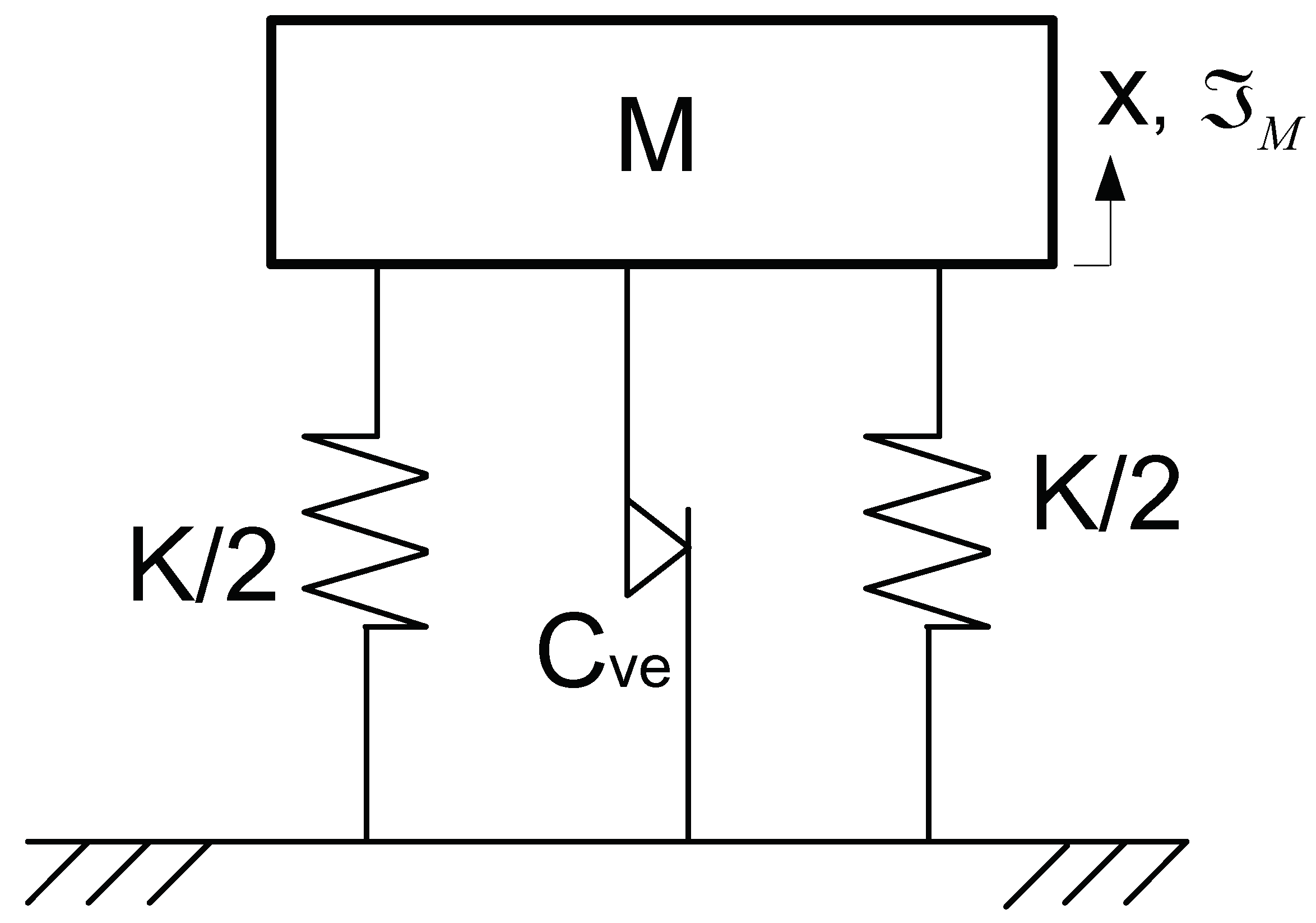
Figure 1 illustrates a single degree-of-freedom system of mass M and stiffness K with a Coulomb friction damper of equivalent viscous damping factor $C_{ve}$ excited by a harmonic force of amplitude ${\Im }_M$.

General form of steady state vibration amplitude under harmonic excitation frequency, $\omega$, can be represented as

$$X={\displaystyle \frac{{\Im }_M}{\sqrt{{\left(K-{\omega }^{2}M\right)}^2+{\left(\omega C_{ve}\right)}^2}}}$$

(1)

Its energy dissipation per cycle is

$$\Delta E_{ve}=\pi \omega C_{ve}{X}^2$$

(2)

Its motion equation can be written as

$$M\ddot{x}+C_{ve}\dot{x}+Kx={\Im }_M$$

(3)

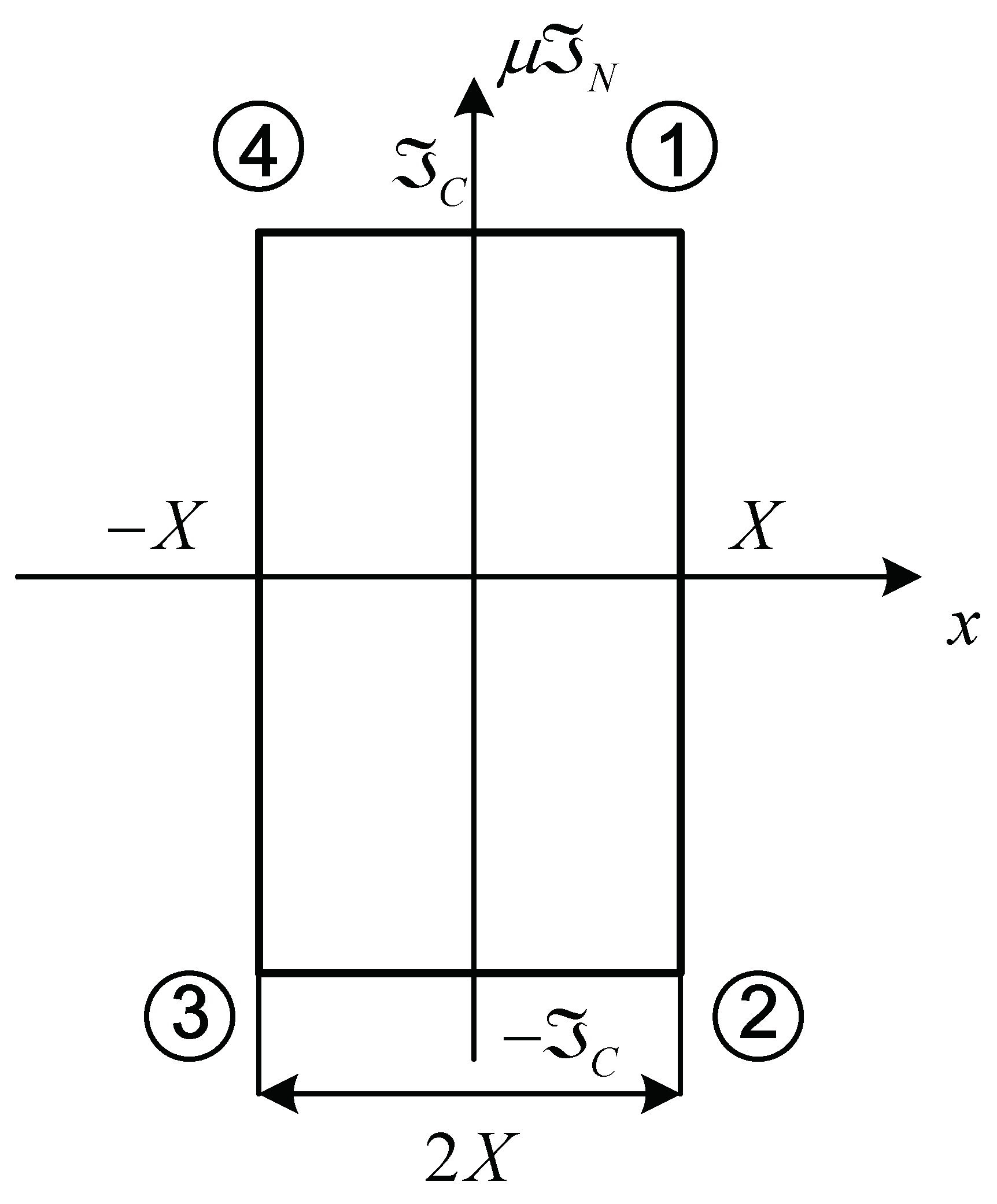
When only Coulomb friction is considered, its hysteresis loop being rectangular as shown in Figure 2.

Its energy dissipation per cycle is

$$\Delta E_c=4\mu {\Im }_{N}X$$

(4)

where $\mu$ is friction coefficient, and ${\Im }_N$ is damper normal force. Under constant normal force ${\Im }_C=\mu {\Im }_N$ and equating Eqs.(2,4), one can obtain

$$C_{ve}=4{\Im }_C\left(\pi \omega X\right)$$

(5)

Substituting $C_{ve}$ of Eq. (5) to Eq.(1), its transmissibility can be written as

$${\displaystyle \frac{XK}{{\Im }_M}}=\sqrt{{\displaystyle \frac{1-{\left(4\mu f_M/\pi \right)}^2}{1-{\lambda }^2}}}$$

(6)

where $f_M={\Im }_N/{\Im }_M$ is the excitation force ratio, $\lambda =\omega /{\omega }_n$ is the frequency ratio. In Eq.(6), singularity exist at $\lambda$ =1 leading to its infinite amplitude of the mass M at resonance.

Furthermore, we can investigate the transmissibility of tradition viscous damper using Eq.(1). By extracting K, its becomes

$$X={\displaystyle \frac{{\Im }_M}{K\sqrt{{\left(1-{\lambda }^2\right)}^2+{\left(\omega C_v/K\right)}^2}}}$$

(7)

in which constant viscous damping ratio is $C_v$. Without loss of generosity, one can assume that the building behaving as resonance at maximum displacement. Hence $\lambda$ =1, while the maximum transmissibility becomes

$$H_v={\displaystyle \frac{XK}{{\Im }_M}}={\displaystyle \frac{1}{{\omega }_n{C}_v/K}}={\displaystyle \frac{K}{{\omega }_n{C}_v}}={\displaystyle \frac{\sqrt{KM}}{C_v}}$$

(8)

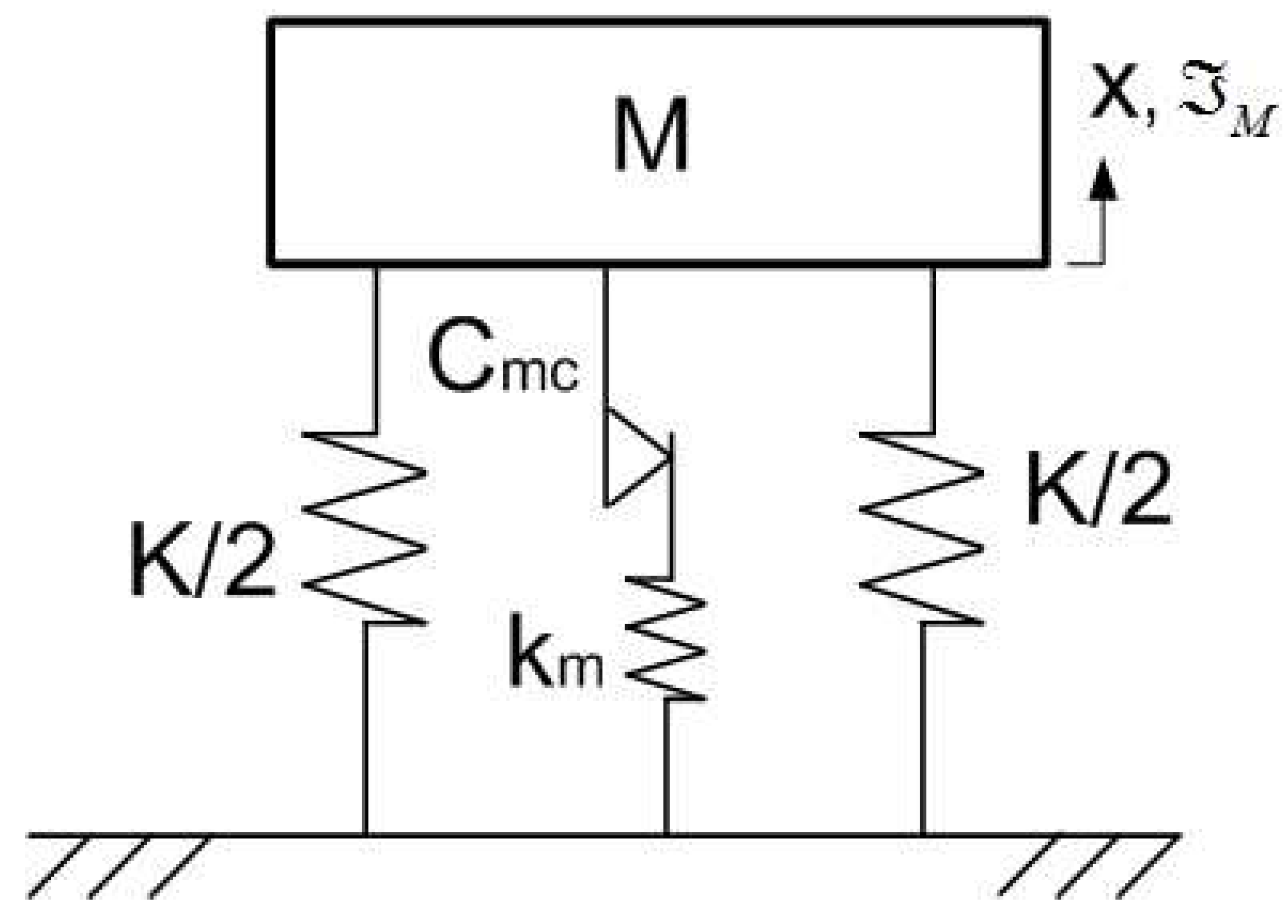
2.2. System Modelling of Maxwell Coulomb Friction Damper

Figure 3 illustrates a single degree-of-freedom system of mass M and stiffness K with a Maxwell Coulomb (MC) friction damper by connecting the Coulomb damper of equivalent damping $C_{mc}$ with the spring of stiffness $k_m$ in series excited by a harmonic force of amplitude ${\Im }_M$.

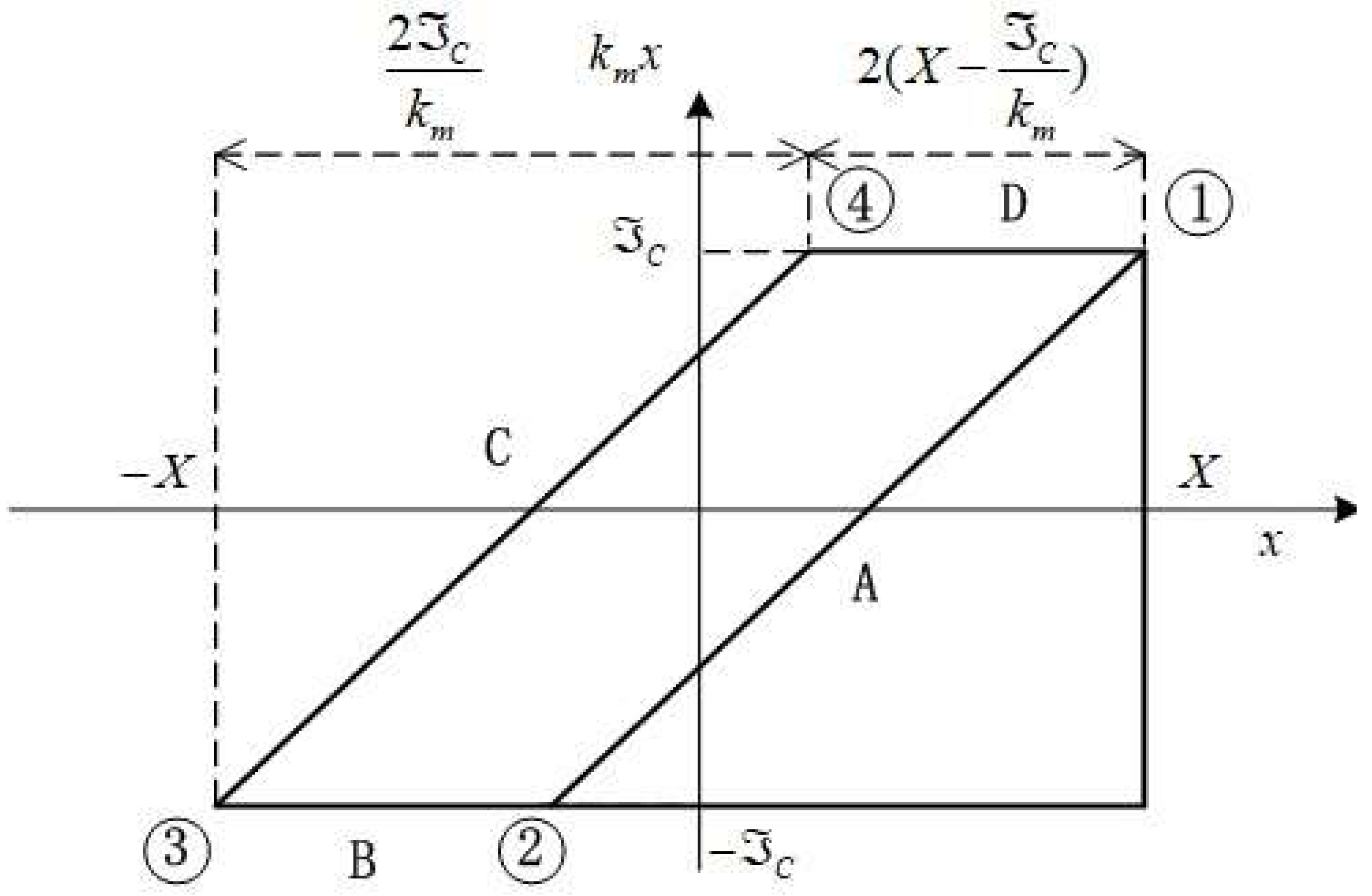
Its motion details are illustrated by the hysteresis loop in Figure 4. Starting from the stick motion in Case A, one can balance the forces acting on the system mass M without the Coulomb element to establish its equation of motion.

Case A: $X\ge x>X-2{\Im }_C/k_m$ from 1 to 2 is the stick motion in which Maxwell spring force is balanced as

$${\Im }_S={\Im }_C-k_m\left(X-x\right)$$

(9)

where ${\Im }_C=\mu {\Im }_N$ is Coulomb damping force amplitude, $\mu$ is friction coefficient, ${\Im }_N$ is damper normal force. $X$ is the system motion amplitude. Its equation of motion becomes

$$M\ddot{x}+Kx+{\Im }_S={\Im }_M$$

(10)

where ${\Im }_M$ is the excitation force applied directly on the system mass. In the numerical ordinary differential equation, one can set

$$x_1=x, x_2=\dot{x}$$

(11)

Rewrite Eq.(10) as

$$\begin{array}{c}{\dot{x}}_2=-\left(K+k_m\right)x_1/M+\left(k_m{X}_r-\mu {\Im }_N+{\Im }_M\right)/M\\ =-\left({\omega }_n^2+{\omega }_a^2\right)x_1/M+\left(k_m{X}_r-\mu {\Im }_N+{\Im }_M\right)/M\end{array}$$

(12)

where ${\omega }_n=\sqrt{K/M}$, ${\omega }_a=\sqrt{k_m/M}$. On the other hand, Coulomb damping is generated by Coulomb element $C_{mc}$ only in the Maxwell arrangement. In this sliding motion, the forces acting on the system mass M are balanced by neglecting the Maxwell spring element.

Case B: $X-2{\Im }_C/k_m\ge x>-X$ from 2 to 3

$$M\ddot{x}+C_{mc}\dot{x}+Kx={\Im }_M$$

(13)

in which Coulomb damping factor $C_{mc}=\mu {\Im }_N/\left|\dot{x}\right|$. Rewrite Eq.(13) as

$$\begin{array}{c}{\dot{x}}_2=-\mu {\Im }_N{x}_2/\left|x_2\right|M-K{x}_1/M+{\Im }_M/M\\ =-\mu {\Im }_N{x}_2/\left|x_2\right|M-{\omega }_n^2{x}_1+{\Im }_M/M\end{array}$$

(14)

In the reverse motion, Case C from 3 to 4 $-X\le x<-X+2{\Im }_C/k_m$, its Maxwell spring force becomes

$${\Im }_S=-{\Im }_C+k_m\left(X+x\right)$$

(15)

Substituting into Eq.(10) and using Eq.(11), we can write

$$\begin{array}{c}{\dot{x}}_2=-\left(K+k_m\right)x_1/M+\left(-k_{m}X+\mu {\Im }_N+{\Im }_M\right)/M\\ =-\left({\omega }_n^2+{\omega }_a^2\right)x_1/M+\left(-k_{m}X+\mu {\Im }_N+{\Im }_M\right)/M\end{array}$$

(16)

Case D is from 4 to 1 with $-X+2{\Im }_C/k_m\le x<X$. Its equation of motion can be established using Eq.(14). These four cases from A to D are combined individually and consecutively to construct the hysteresis loop as shown in Figure 4.

In the combined model with the four different sets of motion, its energy dissipation per cycle is computed using its hysteresis loop in Figure 4 as

$$\begin{array}{ll}\Delta E_{mc}& =4X{\Im }_C-\left({\displaystyle \frac{2{\Im }_C}{k_m}}\right)\left(2{\Im }_C\right)\\ & =4\mu {\Im }_N\left(X-{\displaystyle \frac{\mu {\Im }_N}{k_m}}\right)\end{array}$$

(17)

Equating this to Eq.(2), its equivalent viscous damping factor is derived as

$$C_{ve}={\displaystyle \frac{4\mu {\Im }_N}{\pi \omega X^2}}\left(X-{\displaystyle \frac{\mu {\Im }_N}{k_m}}\right)$$

(18)

Substituting this $C_{ve}$ into Eq.(1), we can establish its motion amplitude as

$$X={\displaystyle \frac{{\Im }_M}{\sqrt{{\left(K-{\omega }^{2}M\right)}^2+{\left[\frac{4\mu {\Im }_N}{\pi X^2}\left(X-\frac{\mu {\Im }_N}{k_m}\right)\right]}^2}}}$$

(19)

which can be expressed at resonant $\omega =\sqrt{K/M}$ as

$$\left[{\left({\displaystyle \frac{4\mu {\Im }_N}{\pi }}\right)}^2-{\Im }_M^2\right]X^2-{\left({\displaystyle \frac{4\mu {\Im }_N}{\pi }}\right)}^2{\displaystyle \frac{2\mu {\Im }_N}{k_m}}X+{\left({\displaystyle \frac{4\mu {\Im }_N}{\pi }}\right)}^2{\displaystyle \frac{{\mu }^2{\Im }_N^2}{k_m^2}}=0$$

(20)

Solving Eq.(20) explicitly using its quadratic solution:

$$X={\displaystyle \frac{-C_2\pm \sqrt{C_2^2-4C_1{C}_3}}{2C_1}}$$

(21)

in which $C_1={\left({\displaystyle \frac{4\mu {\Im }_N}{\pi }}\right)}^2-{\Im }_M^2$, $C_2=-{\left({\displaystyle \frac{4\mu {\Im }_N}{\pi }}\right)}^2{\displaystyle \frac{2\mu {\Im }_N}{k_m}}$ and $C_3={\left({\displaystyle \frac{4\mu {\Im }_N}{\pi }}\right)}^2{\displaystyle \frac{{\mu }^2{\Im }_N^2}{k_m^2}}$.

From this equation, singularity may exist at resonant frequency, $\omega =\sqrt{K/M}$, where square root term $C_2^2-4C_1{C}_3$ becomes

$$\begin{array}{l}{\left({\displaystyle \frac{4\mu {\Im }_N}{\pi }}\right)}^4{\displaystyle \frac{4{\mu }^2{\Im }_N^2}{k_m^2}}-4\left[{\left({\displaystyle \frac{4\mu {\Im }_N}{\pi }}\right)}^2-{\Im }_M^2\right]{\left({\displaystyle \frac{4\mu {\Im }_N}{\pi }}\right)}^2{\displaystyle \frac{{\mu }^2{\Im }_N^2}{k_m^2}}\\ ={\left({\displaystyle \frac{4\mu {\Im }_N}{\pi }}\right)}^2{\displaystyle \frac{4{\mu }^2{\Im }_N^2{\Im }_M^2}{k_m^2}}\end{array}$$

(22)

Substituting back to Eq.(21)

$$X={\displaystyle \frac{{\left(\frac{4\mu {\Im }_N}{\pi }\right)}^2\frac{2\mu {\Im }_N}{k_m}\pm \left(\frac{4\mu {\Im }_N}{\pi }\right)\frac{2\mu {\Im }_N{\Im }_M}{k_m}}{2\left[{\left(\frac{4\mu {\Im }_N}{\pi }\right)}^2-{\Im }_M^2\right]}}$$

(23)

Then its transmissibility becomes

$$\begin{array}{ll}\left|H\left(X\right)\right|& ={\displaystyle \frac{XK}{{\Im }_M}}={\displaystyle \frac{{\left(\frac{4\mu {\Im }_N}{\pi {\Im }_M}\right)}^2\frac{\mu {\Im }_{N}K}{k_m{\Im }_M}\pm \left(\frac{4\mu {\Im }_N}{\pi {\Im }_M}\right)\frac{\mu {\Im }_{N}K}{k_m{\Im }_M}}{{\left(\frac{4\mu {\Im }_N}{\pi {\Im }_M}\right)}^2-1}}\\ & ={\displaystyle \frac{{\left(\frac{4{\zeta }_c}{\pi }\right)}^2\frac{{\zeta }_c}{K_r}\pm \left(\frac{4{\zeta }_c}{\pi }\right)\frac{{\zeta }_c}{K_r}}{{\left(\frac{4{\zeta }_c}{\pi }\right)}^2-1}}={\displaystyle \frac{\frac{4{\zeta }_c^2}{\pi K_r}\left(\frac{4{\zeta }_c}{\pi }\pm 1\right)}{{\left(\frac{4{\zeta }_c}{\pi }\right)}^2-1}}\\ & ={\displaystyle \frac{{\zeta }_c^2}{K_r\left({\zeta }_c\mp \pi /4\right)}}\end{array}$$

(24)

where ${\zeta }_c=\mu {\Im }_N/{\Im }_M$ is Coulomb damping ratio. Two complementary solutions can be obtained from this equation, namely “minus” and “plus” solution in the denominator. From the “minus” solution of Eq.(24), the singular point to avoid is ${\zeta }_c=\pi /4$. When singularity occurs, this solution is complemented by the “plus” solution under nonlinear minimum transmissibility condition (Fung and Chang, 2001). Compared with rigid Coulomb damper, this condition is additional. Therefore, the singularity problem is eliminated in this model. The “plus” and “minus” solutions of Eq.(24) can be plotted in the following three zones:

1) Below the singularity point ${\zeta }_c<\pi /4$, patterns of are very similar. Smaller amplitude is obtained from the “plus” solution as Figure 5.

2) At the singularity point ${\zeta }_c=\pi /4$, the “plus” solution come into play as complementary solution to bring down the large amplitude effects of singularity.

3) Above the singularity point ${\zeta }_c>\pi /4$, one notices that the pattern of “minus” solution is reversed. Contours decrease from the left side. For the “plus” solution, contours increase linearly toward the right side as shown in Figure 5.

3. Numerical Solution and Optimal Design of Turbine Blade

3.1. Numerical Solution on Stick-Slide Motions of Turbine Blade Using Central-Difference Approach

The finite central-difference (CD) approach is one of the simplest discretization techniques and can be used to solve the ODE numerically. Taylor expansion of $x_{i+1}$ and $x_{i-1}$ about point $i$, where $h=\Delta t$

$$x_{i+1}=x_i+h{\dot{x}}_i+{\displaystyle \frac{h^2}{2}}{\ddot{x}}_i+{\displaystyle \frac{h^3}{6}}{\stackrel{⃛}{x}}_i+\dots$$

(25)

$$x_{i-1}=x_i-h{\dot{x}}_i+{\displaystyle \frac{h^2}{2}}{\ddot{x}}_i-{\displaystyle \frac{h^3}{6}}{\stackrel{⃛}{x}}_i+\dots$$

(26)

Adding these equations together

$$x_{i+1}+x_{i-1}=2x_i+h^2{\ddot{x}}_i+\dots$$

(27)

Given the initial value problem $\ddot{x}=f\left(x\left(t\right), \dot{x}\left(t\right),x\left(0\right),\dot{x}\left(0\right)\right)$ and ignoring terms of order 4 or higher

$${\ddot{x}}_i=\left(x_{i-1}-2x_i+x_{i+1}\right)=f\left(x_i,{\dot{x}}_i,t_i\right)$$

(28)

We finally receive the recurrence formula

$$x_{i+1}=h^{2}f\left(x_i,{\dot{x}}_i,t_i\right)-x_{i-1}+2x_i$$

(29)

As we have to generate $x_{i+1}$, backward-difference approximation for ${\dot{x}}_i$ is used:

$${\dot{x}}_i={\displaystyle \frac{x_i-x_{i-1}}{h}}$$

(30)

Applying Eq. (29) developed to Eq. (12) of case A, we can derive ODE as

$$x_{1,i+1}=h^2[-\left({\omega }_n^2+{\omega }_a^2\right)x_{1,i}+\left(k_m{X}_r-\mu {\Im }_N+{\Im }_M\right)/M]-x_{1,i-1}+2x_{1,i}$$

(31)

Similarly for case B, using Eq.(28), one can get

$$x_{1,i+1}=h^2[-{\displaystyle \frac{\mu {\Im }_N}{M}}{\displaystyle \frac{x_{1,i}-x_{1,i-1}}{\left|x_{1,i}-x_{1,i-1}\right|}}-{\omega }_n^2{x}_{1,i}+{\displaystyle \frac{{\Im }_M(t_i)}{M}}]-x_{1,i-1}+2x_{1,i}$$

(32)

Ultimately, the CD form of recurrence equation is

$$x_{1,i+1}^{\text{'}}={\displaystyle \frac{x_{1,i+1}-x_{1,i-1}}{2h}}$$

(33)

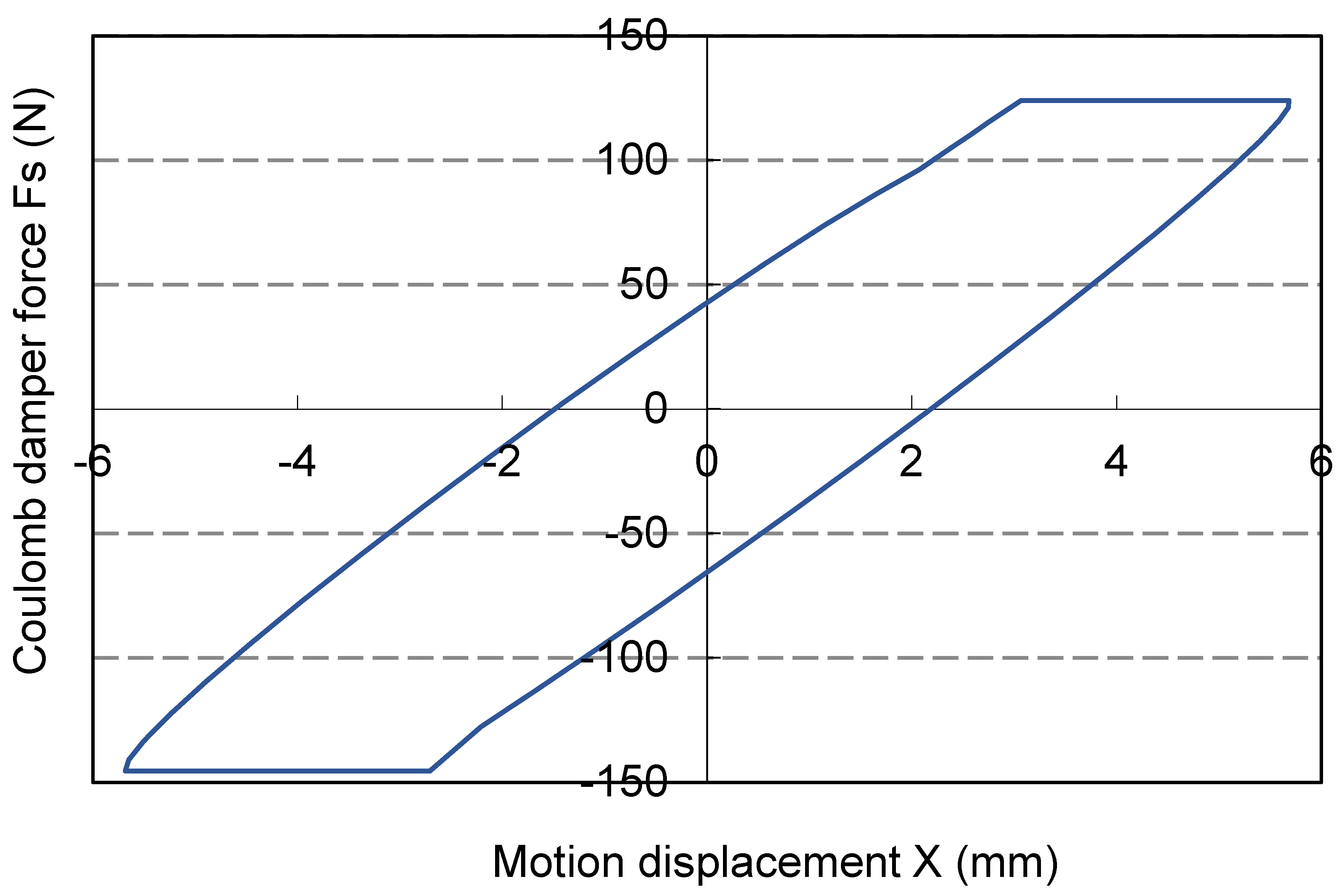
In the analysis of Wang and Chen (1993), turbine blade damper was developed with Maxwell coulomb (MC) arrangement. Similar turbine blade model is simulated with system parameters $M=1.93kg$, $K=10724N/m$, excitation force ${\Im }_M=100N$ at resonant $\omega =1.0{\omega }_n$. For the MC damper, stiffness ratio of its Maxwell spring is $K_r=2.8$, ${\zeta }_c$ = 0.69, $\mu =0.42$. Using the CD method, a MATLAB ODE solver is programmed to simulate its system responses. From its hysteresis loop in Figure 6, one discovers that it is closely correlated with Figure 4 and the theoretical results. For its displacement by Eq.(7), X = 5.8mm, while the simulation displacement from the figure is 5.7mm. Thus the percentage error is only -1.3%. Then the simulated transmissibility $\left|H\left(X\right)\right|$ = 0.610. From Eq.(24), its denominator varies between $-\pi /4$ to $+\pi /4$. Here simulation factor is implemented in the denominator as ${\zeta }_c-\pi f_H/4$. When $f_H$ = 0.53, the percentage error -1.9%. For the damper force comparison, the simulated ${\Im }_C$ = 140N. Meanwhile the theoretical ${\Im }_C$ = 149N which being -5.9% larger. Displacement ratio of stick-slide motions is computed from Figure 4 as $f_{ss}={\displaystyle \frac{k_{m}X-{\Im }_C}{{\Im }_C}}$ = 0.212. And the simulated $f_{ss}$ = 0.238 with +12.2% error. Hence the simulated motion is fully complied with theoretical cases A to D. Hence the accuracy of CD method is fully validated on this blade model.

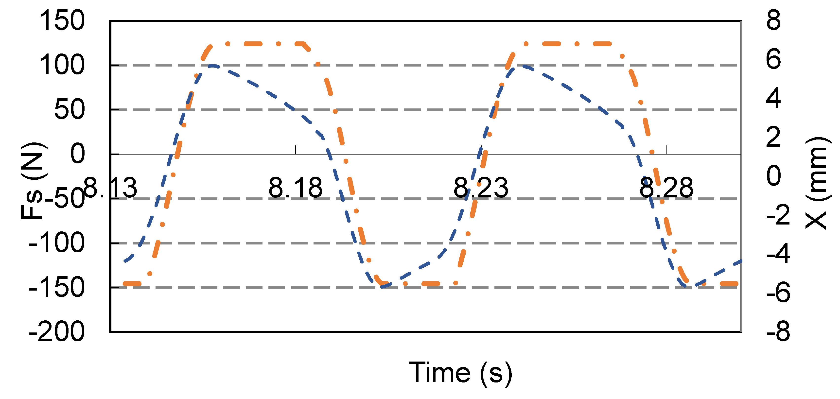
Meanwhile, its motion response is plotted in Figure 7. It rises rapidly under the restoring force of Maxwell spring in stick case C. Then it drops gradually under constant Coulomb force in slide case D. Afterwards, it drops drastically due to the restoring spring force of stick case A. Caused by Coulomb damping force in slide case B, it rises gradually. On the other hand, the damper force is illustrated as Figure 7. Its form is basically similar to that of rigid Coulomb damper which being alternating between high and low levels. The differences are at the switching curves and the lengths of constant levels. Not the same as the straight line for rigid damper, the curves are inclined due to the Maxwell spring. Moreover, the period length follows the sequential order of the motion displacement.

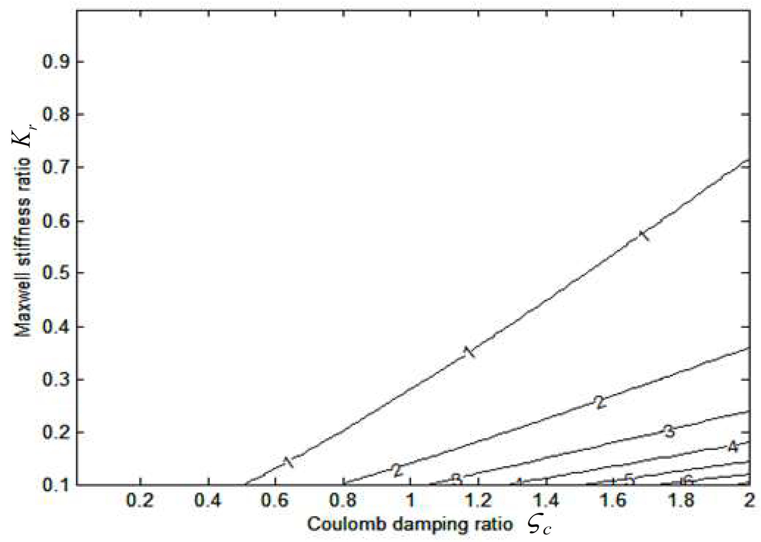
For large range simulation in Figure 8, the contour levels are lower than analytical solution. There is slight vibration level suppression, due to the actual motion. However, some levels are quite accurate such as at level 2 of intercept. Overall, the patterns are closely correlated with the correct model.

3.2. Optimal Contour Design by Central-Difference Unconstrained Search

Although there is no global optimal solution in the contour plot, one can generate its optimal design curve using unconstrained optimization methods, such as Newton search(NS), Gauss-Newton(GN) or Gradient search(GS).

Consider this as unconstrained optimization problem of $\min \left|H\left(X\right)\right|$. Starting from kth design point $X_k$, second-order Taylor expansion of $\left|H\left(X_k\right)\right|$ for an amount of $\delta X_k$ is

$$\left|H\left(X_k+\delta X_k\right)\right|=\left|H\left(X_k\right)\right|+d_k^T\delta X_k+{\displaystyle \frac{1}{2}}\delta X_k^T{Q}_k\delta X_k$$

(34)

in which $Q_k$ is Hessian matrix, $d_k$ is gradient direction. In contour plane, Hessian matrix is defined as

$$Q_k=\left[\begin{array}{cc}{Q}_k^{11}& Q_k^{12}\\ Q_k^{21}& Q_k^{22}\end{array}\right]={\nabla }^2\left|H\left(X_k\right)\right|$$

(35)

where $Q_k^{ij}={\partial }^2\left|H\left(X_k\right)\right|/\partial X_k^i\partial X_k^j$. Meanwhile gradient direction is

$$d_k=-\nabla \left|H\left(X_k\right)\right|$$

(36)

Necessary condition for minimization occurs when direct derivative of $\left|H\left(X_k+\delta X_k\right)\right|$ equal to zero,

$${\displaystyle \frac{d\left|H\left(X_k+\delta X_k\right)\right|}{d\delta X_k}}=d_k^T+Q_k\delta X_k=0$$

(37)

From this equation, one can obtain its descent step directly

$$\delta X_k=-Q_k^{-1}{d}_k^T$$

(38)

Substituting this step into its expansion form, one gets iteration equation

$$X_{k+1}=X_k+\delta X_k$$

(39)

When the data to construct the design path is numerical or experimental, instead of analytical, central-difference form of its gradient direction is used as

$$\nabla \left|H\left(X_k\right)\right|={\left[\begin{array}{cc}\nabla \left|H^i\left(X_k\right)\right|& \nabla \left|H^j\left(X_k\right)\right|\end{array}\right]}^T$$

(40)

where $\nabla \left|H^i\left(X_k\right)\right|={\displaystyle \frac{\left|H\left(X_{k+1}^i\right)\right|-\left|H\left(X_{k-1}^i\right)\right|}{X_{k+1}^i-X_{k-1}^i}}$. Meanwhile, central-difference Hessian is

$$Q_k=\left[\begin{array}{cc}{Q}_k^{11}& Q_k^{12}\\ Q_k^{21}& Q_k^{22}\end{array}\right]$$

(41)

in which $Q_k^{ij}={\displaystyle \frac{\nabla \left|H^i\left(X_{k+1}^j\right)\right|-\nabla \left|H^i\left(X_{k-1}^j\right)\right|}{X_{k+1}^j-X_{k-1}^j}}$, $\nabla \left|H^i\left(X_{k+1}^j\right)\right|$ and $\nabla \left|H^i\left(X_{k-1}^j\right)\right|$ are the gradients at $X_{k+1}^j$ and $X_{k-1}^j$ in ith direction defined in Eq. (40). $X_{k+1}^j-X_{k-1}^j$ is its central-difference in jth direction. Thus $\delta X_k$ in Eq. (38) can be determined using Eqs. (40) and (41). Hence the central-difference Newton search (CDNS) design path can be generated by the iteration scheme in Eq. (39).

Besides CDNS method, the gradient search method (CDGS) is also used to search the design path. Under this method, its descent step is

$$\delta X_k=d_k$$

(42)

In addition, Gauss-Newton method (CDGN) is established by its descent step

$$\delta X_k={\left[\nabla \left|H\left(X_k\right)\right|\times \nabla {\left|H\left(X_k\right)\right|}^T\right]}^{-1}\nabla \left|H\left(X_k\right)\right|\times \left|H\left(X_k\right)\right|$$

(43)

Design paths of these three methods are generated to compare their applicability of contour design in ranges ${\varsigma }_c\subset$ [0, 2.5], $K_r\subset$ [0.1, 0.8] at Figure 8. In the lower range of $K_r$, first path starts from A where $\left|H\left(X\right)\right|$ =3.26 and $K_r=0.1$. For CDNS method, its design curve converges rapidly in three iterations to B with $\left|H\left(X\right)\right|$ =1.21 bounded at $K_r$ =0.3. The reduction in $\left|H\left(X\right)\right|$ is 66%. Its increase in $\det \left(Q_k\right)$ is the fastest from -168 (positive definite) to 0.579 (negative definite). Then design curve of CDGS method converges in four iterations to B’ with $\left|H\left(X\right)\right|$ =0.836.Reduction in $\left|H\left(X\right)\right|$ is 83%. $\det \left(Q_k\right)$ increase from -253 to -5.63 remaining positive definite. For CDGN method, design curve converges vigorously in three iterations to B’’ when $\left|H\left(X\right)\right|$ =1.30. The reduction in $\left|H\left(X\right)\right|$ is 56%. Its $\det \left(Q_k\right)$ decrease from -253 to -18.8 remaining positive definite. Thus fastest increase occurs in CDNS method. For the comparison in ${\varsigma }_c$, the reduction percentages are in the following order: CDGN(4.17%), CDNS(16.7%), CDGS(62.5%). As CDNS is situated at the middle of ${\varsigma }_c$ and $\left|H\left(X\right)\right|$ reduction, it offers the best compensation among these methods. Hence the CDNS path is established in the upper range of $K_r$.It converges convexly from C with $\left|H\left(X\right)\right|$ =2.72 at $K_r$ = 0.3. Then in five steps, it is bounded at D where $K_r$ =0.7 with $\left|H\left(X\right)\right|$ =0.848. Reductions in ${\varsigma }_c$ and $\left|H\left(X\right)\right|$ are 9.52% and 68% respectively. Both cases using CDNS method illustrate that when sufficient $K_r$ reduction are engaged, $\left|H\left(X\right)\right|$ reduction can be much enhanced in this Maxwell arrangement. Simultaneously, ${\varsigma }_c$ is lessened mildly in second path due to the initial position. These paths allow the designs in global ranges to be made up effectively in few steps.

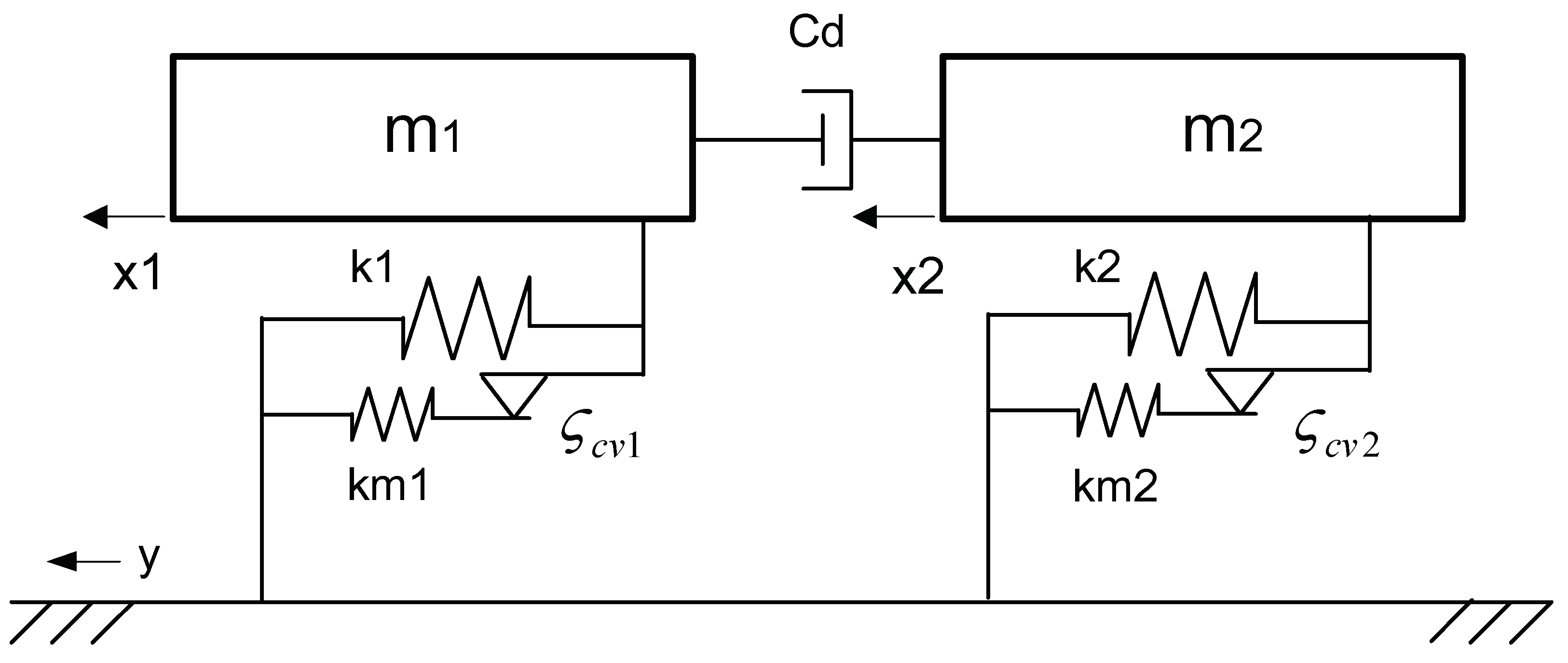
3.3. Performance Evaluation of MC Damper in Seismic Response Design of Adjacent Single-Storey Buildings

In seismic response design (Bhaskararao and Jangid 2007, Chen and Wu 2022, Patel and Jangid 2011), adjacent buildings between single-storey tower(m1) and single-storey podium(m2) are modelled of linear shear type and connected by viscous damper. Its mass-spring-damper model with MC damper is 2DOF as demonstrated in Figure 9. According to the structural parameters of Chen and Wu (2022), m₁ = 3.63×10⁵ kg, $k_1=8.01\times {10}^{5}N/m$. Meanwhile the damping parameters are given by Bhaskararao and Jangid (2007) $c_1=2{\varsigma }_1{m}_1{\omega }_1$ where ${\varsigma }_1={\varsigma }_2=0.02$ are their viscous damping ratios, ${\omega }_1=\sqrt{k_1/m_1}$, $c_2=2{\varsigma }_2{m}_2{\omega }_2$ where ${\omega }_2=\sqrt{k_2/m_2}$. Assume $\mu$ and $\beta$ be the mass and frequency ratios between adjacent buildings. Their ratio parameters are

$$\mu ={\displaystyle \frac{m_1}{m_2}}=1,\beta ={\displaystyle \frac{{\omega }_2}{{\omega }_1}}=2$$

(44)

Let $c_d$ be viscous damping coefficient of connection damper. Then its normalized damping factor is ${\varsigma }_d=c_d/2m_1{\omega }_1$.

Replacing MC dampers ( $k_{m1,2}$, ${\varsigma }_{cv1,2}$ ) with viscous dampers( ${\varsigma }_{1,2}$ ), forms the 2DOF viscous damped with the CD representation:

$$x_1=x_1,x_2={\dot{x}}_1,x_3=x_2,x_4={\dot{x}}_2.$$

(45)

$$x_{1,i+1}=h^2[-2{\varsigma }_1{\omega }_1{x}_{2,i}-2{\varsigma }_d{\omega }_1\left(x_{2,i}-x_{4,i}\right)-{\omega }_1^2{x}_{1,i}+{\Im }_{m1}\left(t_i\right)/m_1]-x_{1,i-1}+2x_{1,i}$$

(46)

$$x_{3,i+1}=h^2[-2{\varsigma }_2{\omega }_2{x}_{4,i}+2\mu {\varsigma }_d{\omega }_2/\beta \left(x_{2,i}-x_{4,i}\right)-{\omega }_2^2{x}_{3,i}+{\Im }_{m2}\left(t_i\right)/m_2]-x_{3,i-1}+2x_{3.i}$$

(47)

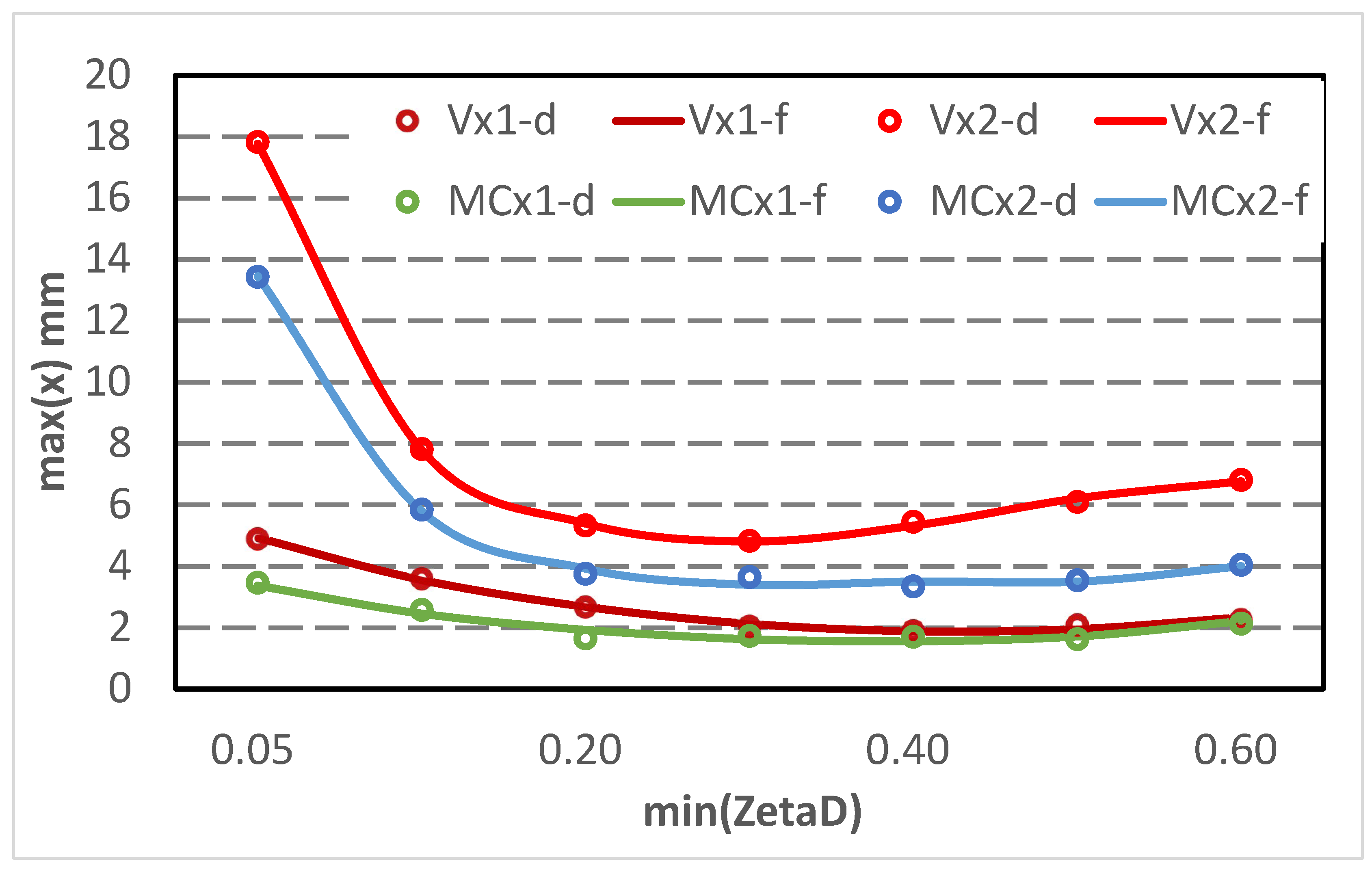
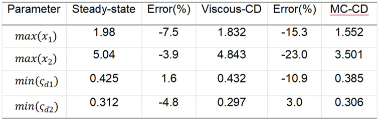
Under seismic acceleration $\ddot{y}$, ground excitations become ${\Im }_{m1,2}=m_{1,2}\ddot{y}\cos \omega t$. Numerical solutions are obtained by tuning harmonic excitation frequency $\omega$. Its seismic responses are recorded at maximum displacement. Moreover, regular increment of ${\varsigma }_d$ is set on each test. Its $\max \left|x\right|$ is plotted against in Figure 10. Its comparisons with those stated by Bhaskararao and Jangid (2007) are listed in Table 1. From this table, its minimum value is obtained as 1.832 which being 7.5% lower than steady-state responses. Meanwhile, its ${\varsigma }_d=0.432$ with 1.6% larger. The discrepancies are due to resolution of data interval and numerical approach of CD ODE. Furthermore for the podium (m2), minimum value is 4.843 with 3.9% lower. And its ${\varsigma }_d$ = 0.297, which being 4.8% smaller. In order to correlate building seismic response using the developed MC damper with that of viscous damper, one can parametric viscous damping ratio $C_v$ by equating their hysteresis energies using Eq.(18)

$$\begin{array}{l}{\displaystyle \frac{C_v}{{\Im }_M}}={\displaystyle \frac{4}{\pi \omega X}}\left[\mu f_r-{\displaystyle \frac{{\left(\mu f_r\right)}^2{\Im }_M}{X{k}_m}}\right]\\ {\displaystyle \frac{\pi \omega X{C}_v}{4{\Im }_M}}={\varsigma }_{cv}-{\displaystyle \frac{{\Im }_M{\varsigma }_{cv}^2}{X{k}_m}}\end{array}$$

(48)

Here $H_v$ is the viscous transmissibility from Eq.(8). Rearranging into quadratic equation,

$${\displaystyle \frac{{\varsigma }_{cv}^2}{K_r{H}_v}}-{\varsigma }_{cv}+{\displaystyle \frac{\pi H_v{C}_v}{4\sqrt{KM}}}=0$$

(49)

Then it is solved as

$${\varsigma }_{cv}={\displaystyle \frac{K_r{H}_v\left(1\pm \sqrt{1-\pi C_v/\left(K_r\sqrt{KM}\right)}\right)}{2}}$$

(50)

Substituting $k_{m1,2}=K_r{k}_{1,2}$ where $K_r=0.3$ and $\mu {\Im }_{N1,2}={\varsigma }_{cv1,2}{\Im }_{m1,2}$ in Eqs.(31,32) to form the loop motion. Then viscous ODE Eqs.(54-47) are transformed to MC ODE by these equations. Utilizing their solutions, maximum displacement curves are generated in Figure 10. Under different resonant frequencies close to their system resonant, damping parameters are generated in Table 1.

From this table, it is interesting to note that max(x) are reduced 15.3 and 23%. Hence the improved performance at lower range for MC damper is validated. Meanwhile, the min( ${\varsigma }_d$ ) ratios remain unchanged. Thus the performance of connection damper is in-altered, MC damper can be applied directly to this structure.

4. Experimental Validation of Optimal Damper Design

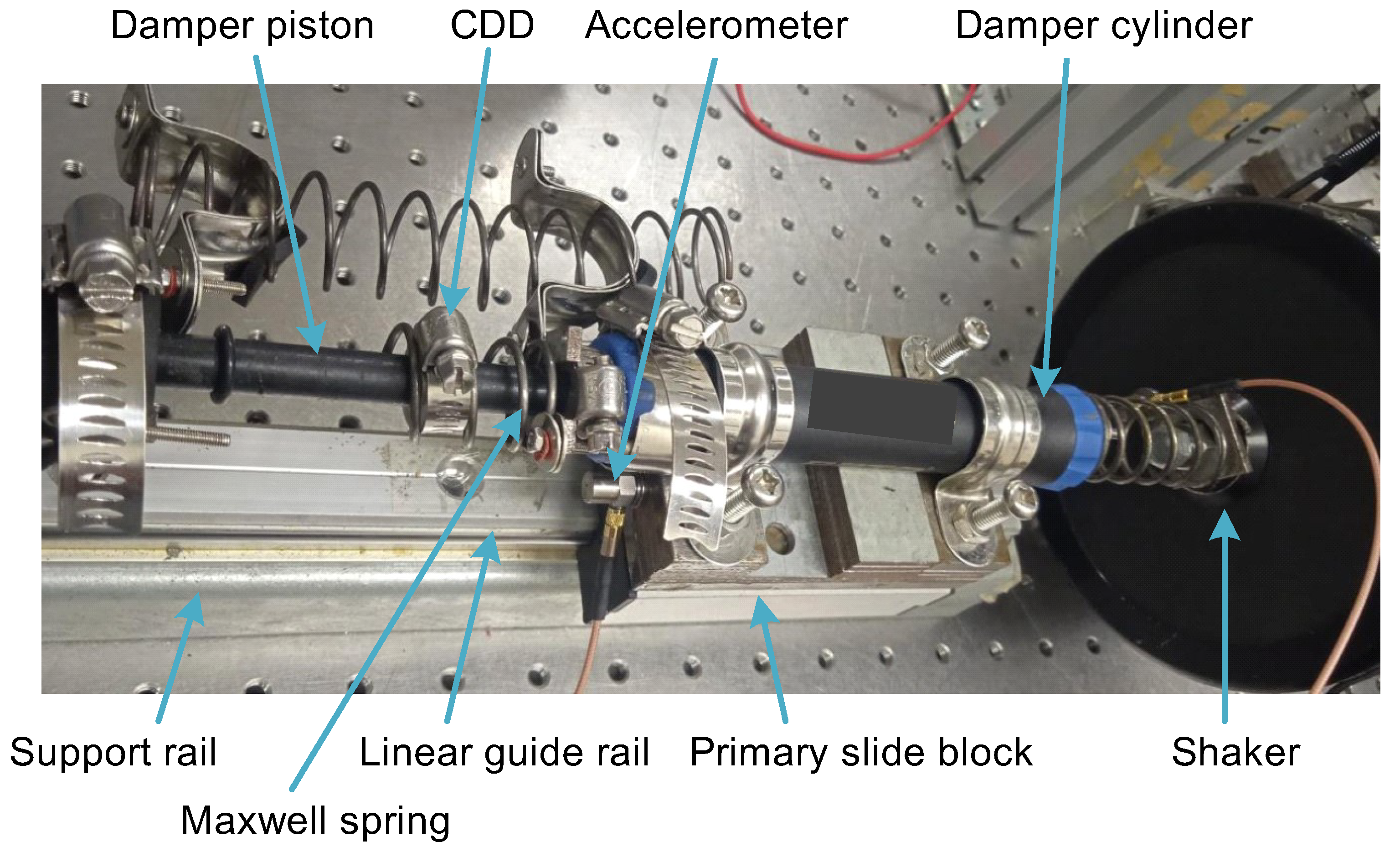
Vibration test is carried out on a spring-mass-damper system to experimentally validate the previous analysis of MC damper with $M=1.235kg$, $K=25160N/m$ at frequency $\omega =0.95{\omega }_n$ which is very close to its resonance. The MC damper is of piston-cylinder type which being well connected to adjustable Maxwell spring and Coulomb damping device (CDD). Linear slide block platform (Wong and Wong, 2021) is established for linear horizontal motion of this system consisted of slide blocks, linear guide rail and support rail as demonstrated in Figure 11.

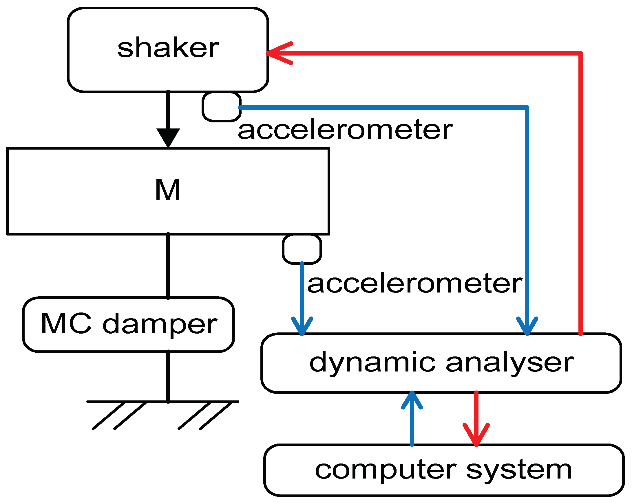
Excitation force is transmitted from the shaker to structural system through shaker spring,

$${\Im }_M=k_s(y-x)$$

(51)

where y is the shaker displacement, $k_s$ is the shaker spring stiffness, y-x is the shaker-damper relative displacement. Schematic of the test-rig is shown in Figure 12. Vibration signals on slide block and shaker are captured by accelerometers. These signals are conditioned at the spectrum analyzer.

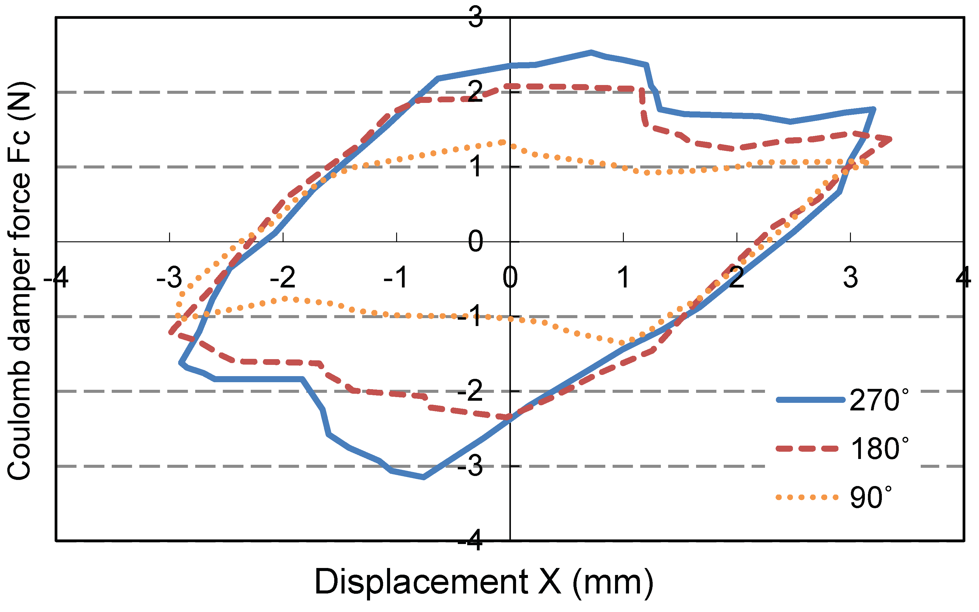
Coulomb damping test is established by increasing the angle of Coulomb damping device (CDD) from 90˚, 180˚ to 270˚ at three coils test. ${\varsigma }_c\subset$ [1.15, 1.36] increases as illustrated in Figure 13. This leads to the increase in hysteresis loop energy from 0.0190J, 0.0317J to 0.0369J. This trend is consistent with the decrease in $\left|H\left(X\right)\right|$ as Figure 5,Figure 9, Figure 14. Slope angle of its principal axis ranges from 39.9˚ to 40.5˚. Deviations are small within 1.8% only. Since there is no change in $K_r$, its slope basically remains the same as Figure 4. Coulomb damping ratio of CDD is calculated by ${\varsigma }_c={\Im }_c/{\Im }_M$.

Using the hysteresis loops in Figure 13, fastening screw tuning Coulomb damping angle ${\theta }_c$ is related to ${\Im }_c$ with Coulomb angle factor $c_f$ and residual damping force $c_r$,

$${\varsigma }_c=\left(c_f{\theta }_c+c_r\right)/k_s(y-x)$$

(52)

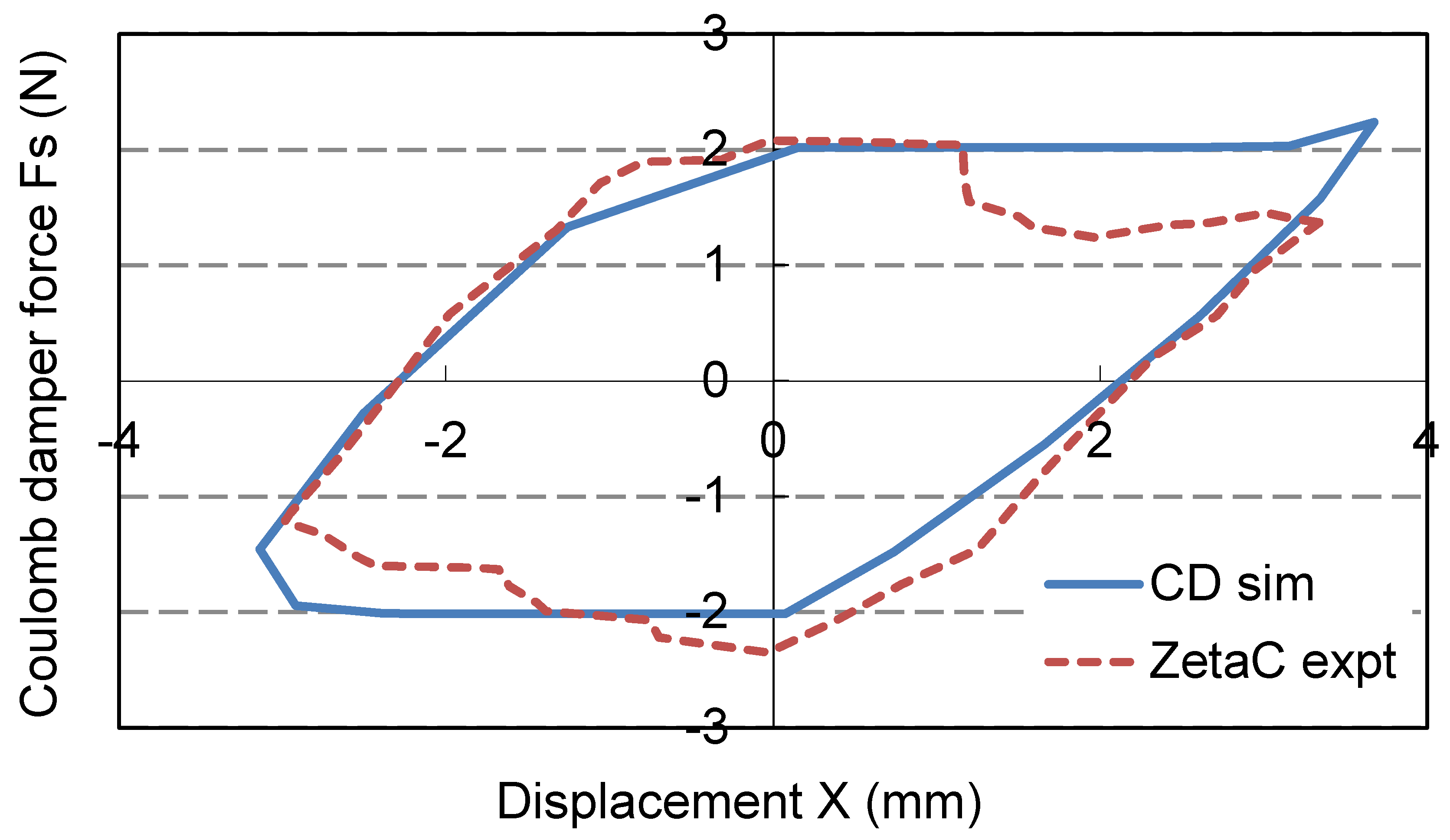
In this line fitting of Coulomb force test, line slope $c_f=6.81\times {10}^{-3}N/\mathrm{deg}$ and line constant $c_r=1.22N$. Meanwhile hysteresis loops at ${\theta }_c$ =180˚ from CD simulation and experiment are compared in Figure 14. Their motions are close to each other. Simulation loop energy 0.0317J with 5.11% deviation from experimental value. For Coulomb damping force, ${\Im }_C=2.02N$ by simulation which is 8.8% deviated from experimental measurement. For experimental sliding motions under this force, they are slightly inclined. This is caused by flexural stiffness of rubber friction plate inside the CDD.

On the other hand in the Maxwell spring test, one can decrease the Maxwell spring coil number from 4, 3 to 2 (which is 7 in K with same helical spring dimensions) i.e. $K_r\subset$ [1.75, 3.50], while keeping the Coulomb device at 90˚. Its hysteresis loop energy ${\mathrm{H}}_{Kr}$ increases from 0.0214J, 0.0387J to 0.0776J. Simultaneously, slope angle of its principal axis increases from 31.7˚, 37.8˚ to 48.5˚. From Figure 4, theoretical slope angle $\theta$ is computed as

$$m=\tan \theta =k_m$$

(53)

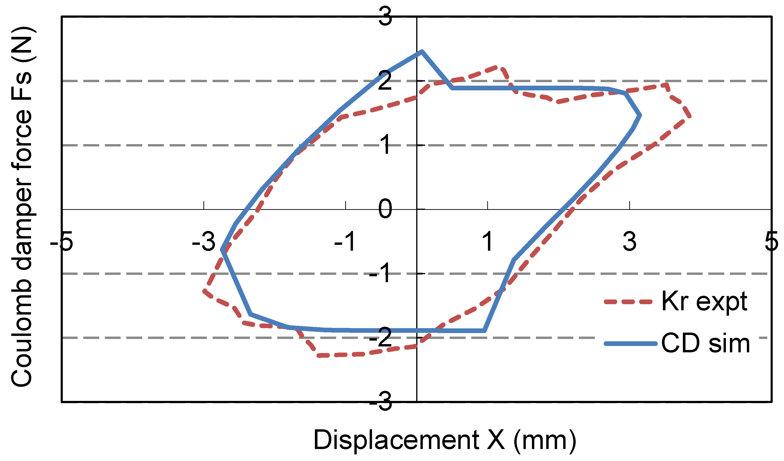
For this spring-mass system, theoretical $\theta$ are 32.7˚, 40.6˚ and 52.1˚ respectively. Comparing with experimental $\theta$, their percentage errors are 3.24 to 7.58%. Hence $\theta$ is validated using Eq.(53). Next is to compare with the CD simulation using the experimental data. From hysteresis plot of three coils test in Figure 15, one discovers that both loops are well matched. Simulation $\theta$ is 36.5˚ with 11.3% error from theoretical $\theta$. Meanwhile ${\mathrm{H}}_{Kr}=0.0375J$, which is only 3.1% deviated from experimental result.

Taking even-interval tests of ${\theta }_c$ and Maxwell spring coil number, their experimental $\left|H\left(X\right)\right|$ record is obtained. The corresponding values in ${\varsigma }_c$ are computed using line fit of Eq.(39). Meanwhile $K_r$ are computed using the coil numbers of Maxwell spring. Inputting this record to MatLab program generates the experimental contour plot in Figure 16.

${\varsigma }_c\subset$ [1.15, 1.36], $K_r\subset$ [1.75, 3.50].

To check applicability of this plot in local ranges ${\varsigma }_c\subset$ [1.15, 1.36], $K_r\subset$ [1.75, 3.50], design paths are established using different ODE approaches, namely, the forward difference (FD), backward difference (BD) and central difference (CD) approaches. In the lower range of $\left|H\left(X\right)\right|$, first design path starts from E where $\left|H\left(X\right)\right|$ =0.465. Maxwell three coils spring is used with its stiffness ratio $K_r$ = 2.33. Meanwhile ${\theta }_c$ is turned to 135˚, and ${\varsigma }_c$ =1.23 as obtained by Eq. (52). Using CDNS approach, its design path is circled line from E to F. It converges from E in five steps to F with $\left|H\left(X\right)\right|$ =0.292 bounded at two coils spring with $K_r$ =3.50. ${\theta }_c$ is minimized to 100˚ with ${\varsigma }_c$ =1.17. Reduction in $\left|H\left(X\right)\right|$ is 69%. Due to constant curvature of $\left|H\left(X\right)\right|$ contour in separate ranges, pattern of $\delta X_k$ varies linearly. Meanwhile $\det \left(Q_k\right)$ increases vigorously from -21.0 to -2.74, indicating that the increase is significant. By the FDNS approach, its path is bounded at ${\varsigma }_c$ =1.17 at second iteration. At this point, ${\varsigma }_c$ reduction is 4.10% and $\left|H\left(X\right)\right|$ reduction is only 21.7%. Additionally, $\det \left(Q_k\right)$ is close to zero, indicating that the increase is insignificant. Similar result is obtained by BDNS approach. Hence the CDNS approach is most accurate and effective in these experimental ranges.

For second design path in the upper range of $\left|H\left(X\right)\right|$, it converges from G where $\left|H\left(X\right)\right|$ =0.707at four coils spring with $K_r$ =1.80. ${\theta }_c$ is at 270˚ with ${\varsigma }_c$ =1.36. It is bounded at Hat the third step with $\left|H\left(X\right)\right|$ =0.515 where $K_r$ =2.33 for three coils spring. ${\theta }_c$ is minimized to 215˚ with ${\varsigma }_c$ =1.32. Ultimately, $\left|H\left(X\right)\right|$ is reduced 27%.From the analytical solution, its contour decreases monotonically from 0.75 to 0.35. Comparing with the experimental contour as Figure 15, it is also monotonic decreasing from 0.65 to 0.40. Hence the experimental contour is closely correlated.

5. Conclusions

Structural model Maxwell Coulomb friction damper is established using damping energy approach. CD ODEs on combined motions are applied on turbine blade vibration isolation. Its simulated motion parameters X(6mm), ${\Im }_C$ (150N), $f_{ss}$, $\left|H\left(X\right)\right|$ are deviated from -1.3% to +12.2% from computed results. Using the CDNS method with CD solver, global range designs of the proposed damper can be achieved on its simulated contour plot with reduction of resonant vibration amplitude of the SDOF primary system up to 66% in just a few iteration steps. In seismic response design of adjacent single-storey buildings (M and ${\Im }_C$ in ranges of $3.5\times {10}^{5}kg$ and 750N), equivalent Coulomb damping ratio is implemented. Maximum displacements are reduced significantly from 15 to 23% at lower damping ratios. Experimental validation of the optimal design of Maxwell Coulomb friction damper (X and ${\Im }_C$ in ranges of 4mm and 3N) is carried out with a prototype of the proposed damper mounted on a linear slide block platform. Close correlation with its numerical predictions is observed in its contour plot of resonant vibration amplitude of the primary system at different values of friction and stiffness of the proposed damper. Its contour plot of the maximum transmissibility with different values of friction force ratio and stiffness ratio is validated by analytical solution. Bounded CDNS paths allow experimental designs in local range on their actual contour plot with maximum reduction of resonant vibration amplitude of 69% in just three to five iteration steps.

References

- Bhaskararao, A.V.; Jangid, R.S. Optimum viscous damper for connecting adjacent SDOF structures for harmonic and stationary white-noise random excitations. Earthquake Engineering and Structural Dynamics 2007, 36, 563–571. [Google Scholar] [CrossRef]
- Brizard, D.; Besset, S.; Jézéquel, L.; et al. Design and test of a friction damper to reduce engine vibrations on a space launcher. Arch. Appl. Mech. 2013, 83, 799–815. [Google Scholar] [CrossRef]
- Chen, P.; Wu, X. Investigations on the Dynamic Response of Adjacent Buildings Connected by Viscous Dampers. Buildings 2022, 12, 1480. [Google Scholar] [CrossRef]
- Fung, R.; Chang, H. Dynamic and energetic analyses of a string/slider non-linear coupling system by variable grid finite difference. Journal of Sound and Vibration 2001, 239, 505–514. [Google Scholar] [CrossRef]
- Hatada, T.; Kobori, T.; Ishida, M.; et al. Dynamic analysis of structures with Maxwell model. Earthquake Eng Struct Dynam 2000, 29, 159–176. [Google Scholar]
- Kheiri, M.; Paidoussis, M.P.; Amabili, M.; Epureanu, B.I. Three-dimensional dynamics of long pipes towed underwater, Part 2 Linear dynamics. Ocean Engineering 2013, 64, 161–173. [Google Scholar] [CrossRef]
- Lee, J.; Berger, E.; Kim, J.H. Feasibility study of a tunable friction damper. Journal of Sound and Vibration 2005, 283, 707–722. [Google Scholar] [CrossRef]
- Patel, C.C. Random response analysis of parallel structures coupled with Maxwell damper. ISET Journal of Earthquake Technology 2019, 56, 57–75, Patel CC, Jangid RS (2011) Dynamic response of adjacent structures connected by friction damper.Earthquake and Structures 2: 149-169.Ricciardelli F, Vickery BJ(1999) Tuned vibration absorbers with dry friction damping. Earthquake Engineering and Structural Dynamics 28: 707-723.. [Google Scholar] [CrossRef]
- Sinha, A.; Trikutam, K.T. Optimal vibration absorber with a friction damper. Journal of Vibration and Acoustics 2018, 140, 021015. [Google Scholar]
- Wu, W.X.; Shua, C.; Wang, C.M. Mesh-free least-squares-based finite difference method for large-amplitude free vibration analysis of arbitrarily shaped thin plates. Journal of Sound and Vibration 2008, 317, 955–974. [Google Scholar] [CrossRef]
- Wang, J.H.; Chen, W.K. Investigation of the vibration of a blade with friction damper by HBM. J. Eng. Gas Turbines Power 1993, 115, 294–299. [Google Scholar]
- Wong, C.N.; Chan, K.T. Identification of cooler tubes with tube-to-baffle impacts. Journal of Vibration and Acoustics 1998, 120, 419–425. [Google Scholar] [CrossRef]
- Wong, W.O.; Wong, C.N. Optimal design of Maxwell viscous-Coulomb air damper with a modified fixed point theory. Journal of Vibration and Acoustics 2021, 143, 031002. [Google Scholar]
Figure 1.
Modelling of structural system with a rigid Coulomb friction damper.
Figure 2.
Hysteresis loop of rigid Coulomb damper.
Figure 3.
Modelling of spring-mass by Maxwell Coulomb damper.
Figure 4.
Hysteresis loop of Maxwell spring and Coulomb damper interaction.
Figure 5.
Contour plot of MC damper model addition solution at ranges of [0, 2.0], [0.1, 1.0].
Figure 6.
Hysteresis loop of turbine blade using CD solver.
Figure 7.
x (
) and
ℑs (
) of turbine blade at
λ = 1.0.
Figure 8.
Contour plot of in ranges = [0, 2.5] and = [0.4, 2.0] .
Figure 9.
Seismic response model of adjacent tower and podium subjected to harmonic ground motion.
Figure 10.
Comparison of - by viscous(V) and MC dampers(data(d), curve fitted(f)).
Figure 11.
Linear slide block platform of MC damper.
Figure 12.
Schematic illustration of MC damper test-rig.
Figure 13.
Experimental loop under variation of .
Figure 14.
Simulation and experimental loop comparison at =180˚.
Figure 15.
Simulation and experimental loop comparison at = 2.33.
Figure 16.
Experimental contour plot of in ranges.