Analyzing the Spread and Transformation of Quantum Information in Large Quantum Systems under External Control

1. Introduction:

In large quantum systems, such as gas systems and complex systems, tracking qubit transitions and the propagation of quantum information becomes increasingly difficult. As the size of the system increases, tracking these transitions becomes increasingly complex. These systems have a complex structure, both in terms of their structure and in terms of the quantum entanglements resulting from their exotic properties, whether in random environments or in environments that evolve in a Hamiltonian fashion. Through this study, I aim to provide a mathematical framework for analyzing the evolution of these systems under external control, focusing on quantum entanglement entropy, a measure of the amount of entanglement within a system. In our study, we focus on the growth rate of the entanglement entropy $v_E$. a key indicator that measures the speed of propagation of quantum information within a system. In large quantum systems, such as gas systems and complex systems, it becomes difficult to track the transformations of qubits and the propagation of quantum information. As the size of the system increases, tracking these transformations becomes increasingly complex. These systems have a complex structure, both in terms of their structure and in terms of the quantum entanglements resulting from their exotic properties, whether in random environments or in environments that evolve in a Hamiltonian fashion. Through this study, I aim to provide a mathematical framework for analyzing the evolution of these systems under external control, focusing on the quantum entanglement entropy, a measure of the amount of entanglement within a system. In our study, we focus on the growth rate of the entanglement entropy $v_E$. a key indicator that measures the speed of propagation of quantum information within a system. In large quantum systems of 50 qubits or more, these systems face three basic challenges. The first is the difficulty of tracking the spread of information through entangled qubits over time, the loss of information due to the effects of noise, environment, or chaos, and finally, the entropy reaches its maximum value at $S_{\max }$ after a period of time of $t_c$. The importance of this problem is clearly evident in quantum applications that rely on the transmission of quantum signals, such as quantum computing and quantum communications.

2. Entanglement Entropy Growth:

2.1. Definition of Growth Rate:

The growth rate of the entanglement entropy is defined as follows:

$$v_E={\displaystyle \frac{dS}{dt}}$$

(1)

where S is the entanglement entropy and t is time.

This equation embodies the linear growth of entanglement dynamics, where entropy increases proportionally with time ($S\sim v_{E}t$).

Therefore, $v_E$ is a direct measure of the speed at which quantum information propagates through a system.

2.2. Saturation and Quantum Lyapunov Time:

this mathematical model, it appears that the quantum system is continuously increasing without limit. However, this does not happen in closed quantum systems in reality as the system reaches a saturation point at time $t_c$ and stops growing linearly. This growth explains the speed of propagation of parameters within the quantum system and is directly related to the quantum Lyapunov time ${\lambda }_L$ through the relation

$$C\left(t\right)=e^{{\lambda }_{L}t}$$

(2)

This relationship explains the transition of the system from a state of relative stability to chaos through this exponential relationship. through the Out-of-Time-Order Correlators (OTOC).

2.3. Model System: One-Dimensional Qubit Chain:

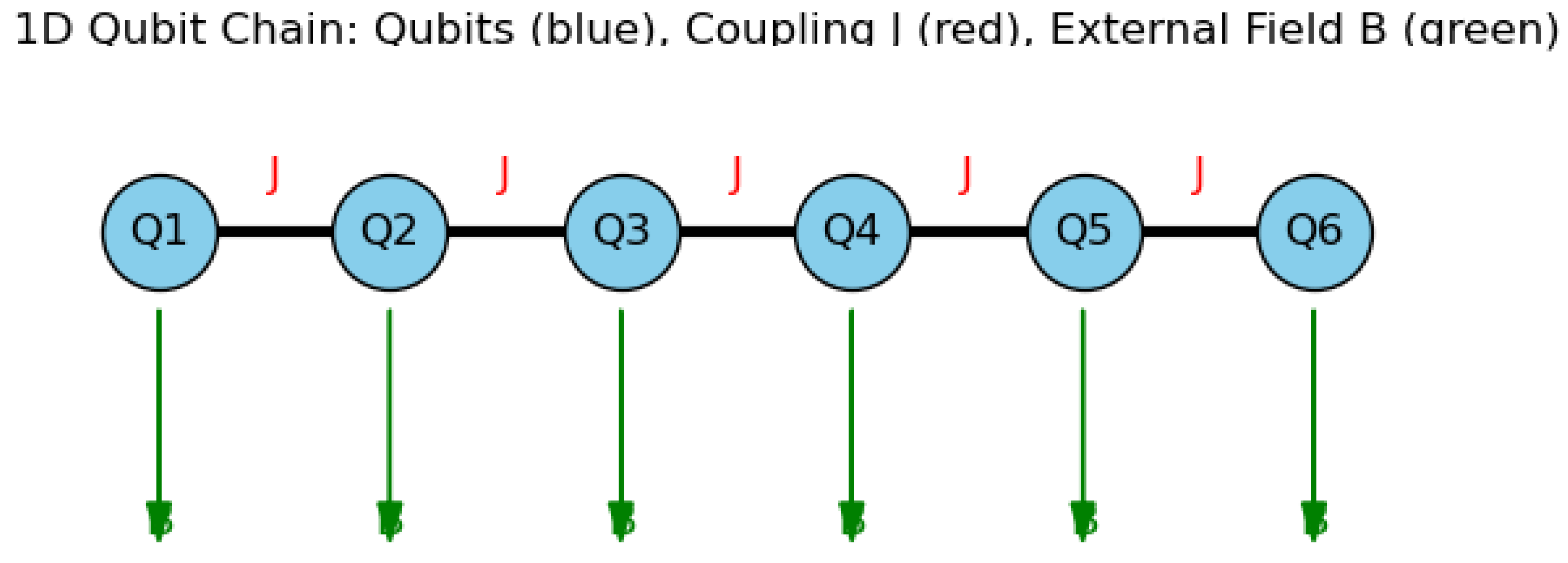
The studied system consists of a one-dimensional (1+1D) form of a linear chain of qubits, which allows us to directly observe the evolution of the system through.

$$H=\sum _{i}J{\sigma }_i^z{\sigma }_{i+1}^z+B{\sigma }_i^x,$$

(3)

where J is the coupling constant between the qubit and the nearest cos, ${\sigma }_i^z{\sigma }_{i+1}^z$ represents the entanglement and $B{\sigma }_i^x$ represents the effect of the external field, which here is the magnetic field

Figure 1. Schematic illustration of a one-dimensional chain of qubits. Each qubit ($Q_1,Q_2,\dots ,Q_6$) is represented as a blue node. Neighboring qubits interact via coupling J (red links), while each qubit is also subjected to an external field B (green arrows). The figure was generated using a Python script (Matplotlib) for visualization purposes.

Figure 1. Schematic illustration of a one-dimensional chain of qubits. Each qubit ($Q_1,Q_2,\dots ,Q_6$) is represented as a blue node. Neighboring qubits interact via coupling J (red links), while each qubit is also subjected to an external field B (green arrows). The figure was generated using a Python script (Matplotlib) for visualization purposes.

2.4. Subsystem Size, Maximal Entropy, and Time Evolution:

The maximum entanglement entropy that a system reaches is when the system is divided into two equal parts. Then the entanglement entropy reaches its maximum value when:

$$S_{max}\approx {\displaystyle \frac{N}{2}}ln2,$$

(4)

where N represents the number of qubits. By studying the stages of system development, we can divide it into two stages: the first is before the start of $t_c$, and the second is after. from (1) by using Heaviside Functions:

(a) Before saturation ($t<t_c$):

$$S_1\left(t\right)=v_{E}t·\theta (t_c-t)$$

(5)

This stage represents the gradual spread of entanglement entropy as quantum information is initially distributed among the qubits.

(b) After saturation ($t\ge t_c$):

$$S_2\left(t\right)=S_{\max }·\theta (t-t_c)$$

(6)

At this stage, the growth rate of entanglement entropy is approaching its maximum. A decline in the value may occur later due to environmental effects, such as environmental fluctuations or measurement inefficiency.

Combined Expression:

Combining both regimes (5), (6), we obtain:

$$S\left(t\right)=v_{E}t·\theta (t_c-t)+S_{\max }·\theta (t-t_c)$$

(7)

This shows that the entropy $S\left(t\right)$ grows linearly with rate $v_E$ before the critical time $t_c$, and then saturates at the maximum value $S_{max}$. This behavior is a characteristic feature of quantum thermalization and scrambling.

3. Entanglement Entropy Control:

In real systems under the influence of an external field, the rate of growth of entanglement entropy changes under the influence of this field, which may be variable over time. If $v_E$ is constant, the growth is linear. But under external control or periodic influence:

$$v_E\to v_E\left(t\right)$$

We assume that $v_E$ varies periodically, which makes it possible to write it through Fourier-like :

$$v_E\left(t\right)={ϵ}_0+\sum _n{ϵ}_n{f}_n\left(\omega t\right)$$

The simplest form of oscillation can be written as:

$$v_E\left(t\right)={ϵ}_0+{ϵ}_{1}cos\left(\omega t\right)+{ϵ}_2{sin}^2\left(\omega t\right)$$

In quantum systems, phase locking allows us to transform the time dependence into a precise phase dependence ${\varphi }_{\mathrm{ctrl}}$

$$v_E^{\mathrm{controlled}}=v_E^{\left(0\right)}-\Delta v·cos\left({\varphi }_{\mathrm{ctrl}}\right)$$

(8)

${\varphi }_{\mathrm{ctrl}}$ represents an adjustable control parameter (such as the laser phase or magnetic field angle). When ${\varphi }_{\mathrm{ctrl}}=0$, the damping is maximum. When ${\varphi }_{\mathrm{ctrl}}=\pi /2$, the control has no effect.

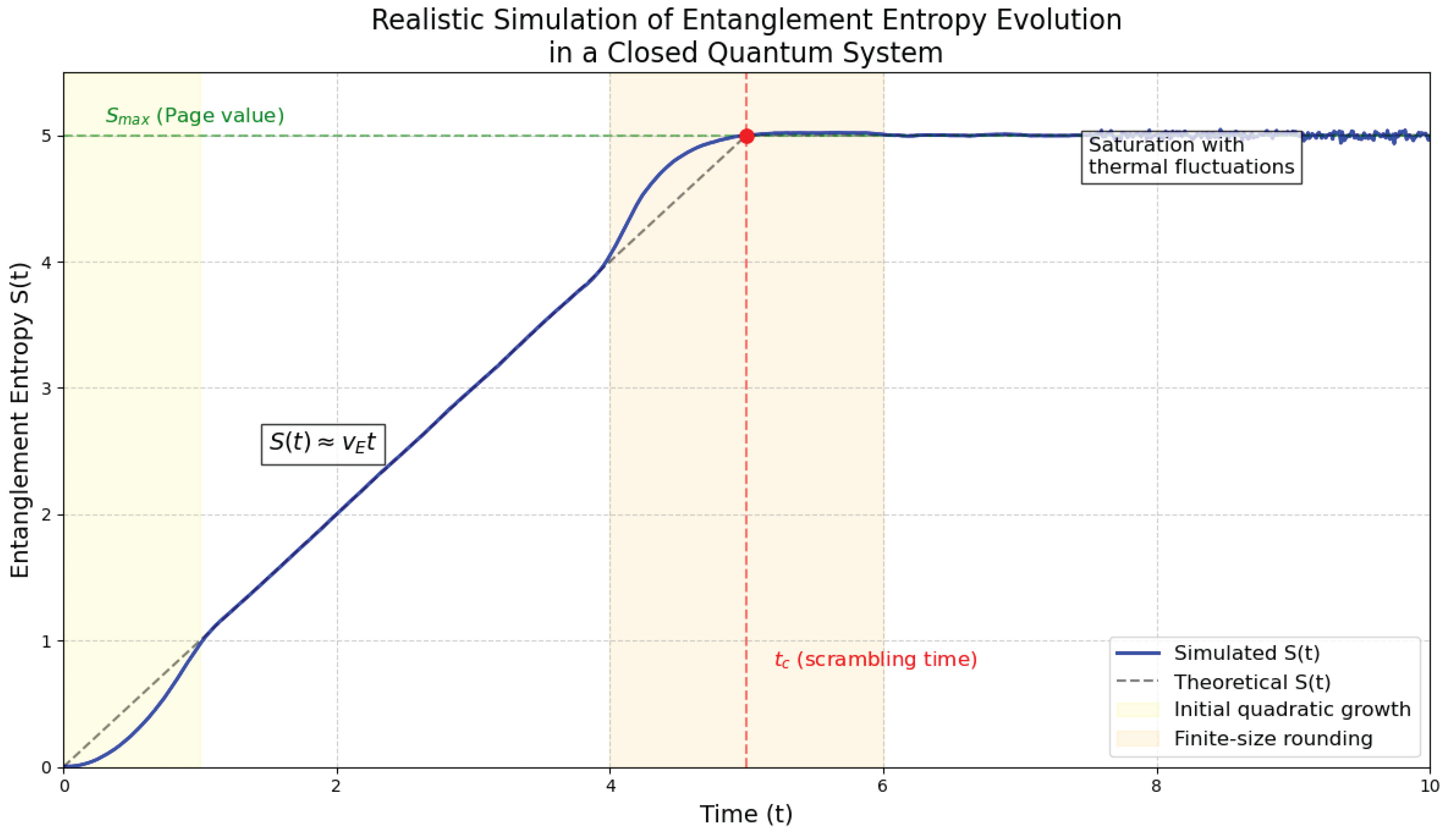
Figure 2. Realistic simulation of the entanglement entropy evolution $S\left(t\right)$ in a closed quantum system. The dashed black curve shows the idealized theoretical behavior: linear growth $S\left(t\right)\approx v_{E}t$ until the scrambling time $t_c$, followed by saturation at the Page value $S_{\max }$. The solid blue curve incorporates more realistic physical effects: (i) an initial quadratic growth phase, (ii) finite-size rounding near the critical time $t_c$, (iii) stochastic quantum fluctuations, and (iv) late-time thermal fluctuations around $S_{\max }$. Shaded regions highlight the corrections to the idealized model.

Figure 2. Realistic simulation of the entanglement entropy evolution $S\left(t\right)$ in a closed quantum system. The dashed black curve shows the idealized theoretical behavior: linear growth $S\left(t\right)\approx v_{E}t$ until the scrambling time $t_c$, followed by saturation at the Page value $S_{\max }$. The solid blue curve incorporates more realistic physical effects: (i) an initial quadratic growth phase, (ii) finite-size rounding near the critical time $t_c$, (iii) stochastic quantum fluctuations, and (iv) late-time thermal fluctuations around $S_{\max }$. Shaded regions highlight the corrections to the idealized model.

4. Effective Accumulated Entropy Growth Over Time:

To model the entropy growth rate while incorporating a weighting factor that reflects physical limitations or inefficiencies of observational instruments. From (1):

$${\displaystyle \frac{dS}{dt}}=v_E\left(t\right)\Rightarrow S\left(t\right)=\int v_E\left(t\right)dt$$

(9)

$$S_{\mathrm{eff}}\left(t\right)={\int }_0^t\kappa \left(\tau \right)·v_E\left(\tau \right)d\tau$$

(10)

where $\kappa \left(t\right)\in [0,1]$ It represents the weighting factor of physical constraints or inefficiency of monitoring instruments. by Integrate Controlled Growth from (8) and (9) we find:

$$S_{\mathrm{growth}}(t,\varphi )={\int }_0^t\left[v_E^{\left(0\right)}-\Delta vcos\varphi \right]d\tau$$

(11)

Exchange function:

$$\kappa \left(\varphi \right)={\kappa }_0\left(1+\beta cos\varphi \right)$$

(12)

By defining the exchange function, we determine the difference according to which stage of the system’s evolution we are studying: before or after saturation. Using Heaviside Functions:

$$\Theta (t,\varphi )=\theta \left(t_c\left(\varphi \right)-t\right)+e^{-\kappa \left(\varphi \right)(t-t_c\left(\varphi \right))}\theta \left(t-t_c\left(\varphi \right)\right)$$

(13)

Integration after saturation exactly:

$${\int }_{t_c}^t\left[v_E^{\left(0\right)}-\Delta vcos\varphi \right]e^{-\kappa \left(\varphi \right)(\tau -t_c)}d\tau ={\displaystyle \frac{\left[v_E^{\left(0\right)}-\Delta vcos\varphi \right]}{\kappa \left(\varphi \right)}}\left(1-e^{-\kappa \left(\varphi \right)(t-t_c)}\right).$$

(14)

Simplified approximate formula:

$$S(t,\varphi )\approx S_{\max }+\left[v_E^{\left(0\right)}-\Delta vcos\varphi \right](t-t_c)e^{-\kappa \left(\varphi \right)(t-t_c)}.$$

Combining the two parts: Thus, the complete formula becomes:

$$\begin{array}{|c|}\hline S(t,\varphi )=\left\{\begin{array}{cc}\left[v_E^{\left(0\right)}-\Delta vcos\varphi \right]t\hfill & t\le t_c\left(\varphi \right)\hfill \\ S_{\max }+\left[v_E^{\left(0\right)}-\Delta vcos\varphi \right]\left(t-t_c\left(\varphi \right)\right)e^{-\kappa \left(\varphi \right)(t-t_c\left(\varphi \right))}\hfill & t>t_c\left(\varphi \right)\hfill \end{array}\right.\\ \hline\end{array}$$

(15)

$$\begin{array}{cc}\hfill t_c\left(\varphi \right)& ={\displaystyle \frac{S_{\max }}{v_E^{\left(0\right)}-\Delta vcos\varphi }}\hfill \\ \hfill \kappa \left(\varphi \right)& ={\kappa }_0\left(1+\beta cos\varphi \right)\hfill \end{array}$$

Figure 3. Controlled entanglement entropy $S(t,\varphi )$ as a function of time for several values of the control parameter $\varphi$. The curves were generated using Python scripts following a piecewise model: linear growth before the saturation time $t_c\left(\varphi \right)$ and exponential decay after $t_c\left(\varphi \right)$, as defined in the main text. These plots serve as illustrative approximations of the theoretical predictions.

Figure 3. Controlled entanglement entropy $S(t,\varphi )$ as a function of time for several values of the control parameter $\varphi$. The curves were generated using Python scripts following a piecewise model: linear growth before the saturation time $t_c\left(\varphi \right)$ and exponential decay after $t_c\left(\varphi \right)$, as defined in the main text. These plots serve as illustrative approximations of the theoretical predictions.

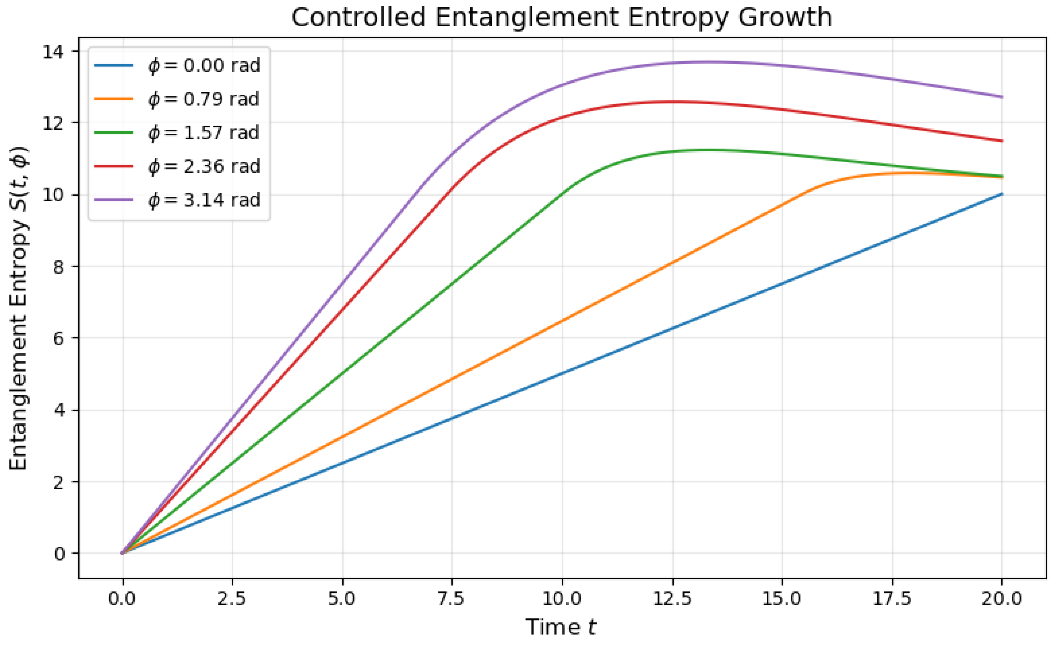
Initially, state $t<t_c$: In this state, the entanglement entropy grows linearly with time. The growth rate is constant and can be controlled using the parameter $phi$.

Second, state $t>t_c$: Growth gradually stops, the entropy approaches its maximum value $S_{max}$, with an exponential decay according to the parameter $kappa\left(\varphi \right)$.

The parameter $\varphi$ allows tuning both the growth rate $\Delta vcos\varphi$ and the saturation time $t_c\left(\varphi \right)$.

5. Conclusions:

In this paper, we extend the scope of the standard entanglement entropy dynamics for large quantum systems. In quantum systems, the dynamics are typically characterized by two phases: a linear growth phase before reaching saturation and a post-saturation phase. Here, we highlight these quantum behaviors, but under the influence of external control or environmental effects. In this paper, we present a framework for working using a control parameter ${\varphi }_{\mathrm{ctrl}}$, which allows us to control the rate of entropy growth, as well as introducing the parameter $\kappa \left(\varphi \right)$, which allows us to include environmental effects, measurement inefficiency, and loss of coherence after saturation, which are important measurements.